A Construction of Rational Seifert Surface in Lens Space

Abstract

In this note, we give a method to construct rational Seifert surface for those smooth or piece-wise linear oriented knots in Lens space $L(p,q)$. We assume that the oriented knot has a regular projection on Heegaard torus and then construct rational Seifert surface on twist toroidal diagram.

1 Introduction

The existence of Seifert surface of a null-homologous knot or link is a very interesting problem in topology. In chapter.5.A.4[1], Rolfsen showed us a direct way to constructing Seifert surface by regular projection of a smooth or piece-wise linear knot. It’s a natural question whether we can generalize Seifert surface of a link. In section 1 of[2] ,Kenneth Baker and John Etnyre defined rational Seifert suface for a knot which represents a torsion element in homology group $H_{1}$. Especially, $H_{1}(L(p,q))=\mathbf{Z}_{p}$. Thus,every knot represents a torsion element in homology group. We give a construction of rational Seifert surface for arbitrary smooth knot when it has a regular projection on Heegaard torus of $L(p,q)$. We assume that all knots mentioned in this note are smooth or piece-wise linear.

2 Representation of a smooth knot in L(p,q)

Let $V_{i},(i=1,2)$ be two solid torus $D^{2}\times S^{1}$. Its meridian and longitude is denoted by$(\mu_{i},\lambda_{i})$. Then, in the sense of Heegaard decomposition, a lens space $L(p,q)$ can be described by $V_{1}\cup_{\phi}V_{2}$ where the gluing map $\phi:\partial V_{2}\rightarrow V_{1}$  is an orientation-reversing diffeomorphism given in standard longitude-meridian coordinates on the torus by the matrix

$$\begin{pmatrix}-q&q^{\prime}\\ p&-p^{\prime}\end{pmatrix}\in-SL_{2}(\mathbf{Z})$$

In particular, $\phi(\mu_{2})=-q\mu_{1}+p\lambda_{1}$. This fact concludes that $H_{1}(L(p,q))=\langle\lambda_{1}|\leavevmode\nobreak\ p\lambda_{1}=1\rangle$.
 
    Let $K$ be a knot in Lens space $L(p,q)$. Of course, after a small perturbation, it can be disjoint from the core $C_{i}=0\times S^{1}\subset D^{2}\times S^{1}$of two solid torus at the same time. Please notice that $V_{i}\setminus C_{i}$ deformation retracts to its boundary$\leavevmode\nobreak\ \partial V_{i}$. Thus, the deformation retraction $P:L(p,q)\setminus V_{1}\cup V_{2}\rightarrow\partial V_{1}$ projects $K$ onto Heegaard torus $\partial V_{1}$

Definition 1.

(see chapter 3.E of [1])
Assume K is a smooth knot. The deformation retraction $P$ is said to be regular for $K$ iff :
$\forall x\in\partial V_{1},\leavevmode\nobreak\ |P^{-1}(x)|=0,1,2$ and if $2$, $P(K)$ intersects itself transversely at $x$

Remark 1.

if P is not regular for K, then, after a small perturbation of K, P is regular. From now on, We assume K is in the interior of thickened torus $\partial V_{1}\times[-1,1]$ and the natural projection $\partial V_{1}\times[-1,1]\rightarrow\partial V_{1}$ is regular for K. We regard $L(p,q)$ is obtained from $\partial V_{1}\times[-1,1]$ gluing $V_{1}$ to the lower boundary of this thickened torus and $V_{2}$ to the upper boundary.

After above discussions, the reader can realize that such a knot K can be drawn on a fundamental domain of torus $\partial V_{1}$.Notice that $\partial V_{1}=T^{2}=\mathbf{R^{2}}/\mathbf{Z^{2}}$. The usual choice of fundamental domain of this torus is a square $[0,1]\times[0,1]\subset\mathbf{R^{2}}$. In this square, $[0,1]\times\{0\}$ represents $\mu_{1}$ while $\{0\}\times[0,1]$ represents $\lambda_{1}$

Definition 2.

(see Def 2.1 of [3])
The twist toroidal diagram of $\partial V_{1}\subset L(p,q)$ is a fundamental domain in $\mathbf{R^{2}}$ bounded by four straight line:

$$\begin{cases}x=0\\ x=1\\ y=-\frac{q}{p}x\\ y=-\frac{q}{p}(x-1)\end{cases}$$

Remark 2.

In twist toroidal diagram, it’s also holds that $(0,1)(0,0)(1,0)$ represent a same point in $\partial V_{1}$. The straight line $y=-\frac{q}{p}x$ has same direction as $\mu_{2}$.

3 Construction of rational Seifert surface

3.1 Basic Idea

By remark 1, we can draw $K$ on the twist toroidal diagram of $\partial V_{1}$. We want to find a ”cobordism” surface (inside of $\partial V_{1}\times[-1,1]$) from $rK$ to a link $L^{\prime}$ which is the union of several $(\pm\mu_{2})-knot$ in $\partial V_{1}\times\{1\}$ and $(\pm\mu_{1})-knot$ in $\partial V_{1}\times\{-1\}$. Then we attach several meridian discs of $V_{i}$ to this ”cobordism”, this so called ”cobordism” should be a real rational Seifert surface of $K$. We will see later that $L^{\prime}$ may contain several null-homologous component on the upper boundary of $\partial V_{1}\times[-1,1]$.

3.2 Details of the construction

The construction is divided into following steps:

1. Replace crossings of $P(K)$ by short-cut arcs on the twist toroidal diagram. Or equivalently, cut the crossing point $A$ into two points $A_{0,1}$. Then, we get a torus link $L\subset\partial V_{1}\times\{0\}$

   

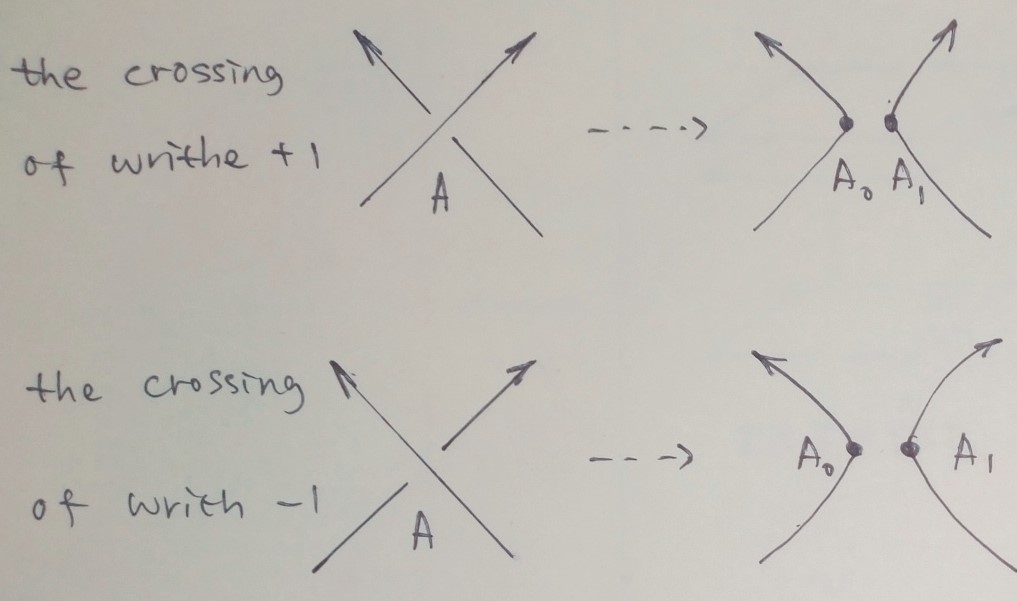
   Figure 1: Make a crossing apart

2. Computations:
   Compute $[K]=[L]\in H_{1}(\partial V_{1})$ in coordinate $(\mu_{1},\lambda_{1})$. Assume that $[L]=n(a\mu_{1}+b\lambda_{1})$ where $n,a,b\in\mathbf{Z},g.c.d.(a,b)=1$. The coefficient $na(nb)$ and can be obtained by counting the algebraic intersection numbers of $L$ and $\lambda_{1}(\mu_{1})$-curve.
   Also, Compute order $r$ of $[K]=[L]\in H_{1}(L(p,q))=\langle\lambda_{1}|p\lambda_{1}\rangle$.
   

   $$r=\frac{p}{g.c.d.(p,nb)}$$

   
   

   Then,

   $$r[L]=rna\mu_{1}+rnb\lambda_{1}=rna\mu_{1}+\frac{rnb}{p}(p\lambda_{1})=rna\mu_{1}+\frac{rnb}{p}(q\mu_{1}+\mu_{2})=(rna+\frac{rnbq}{p})\mu_{1}+\frac{rnb}{p}\mu_{2}$$

3. Construct ”cobordism” from link $L$ to $L^{\prime}$ noticed above.

   1. draw torus link $(rna+\frac{rnbq}{p})\mu_{1}$ on $\partial V_{1}\times\{-1\}$ (denoted by$L^{-}$)and $(-(rna+\frac{rnbq}{p})\mu_{1})$ on $\partial V_{1}\times\{1\}$ s.t both torus link avoid a connected neighborhood of each crossing of $P(K)$ in the diagram where the crossing is now replaced by short-cut arcs.

      

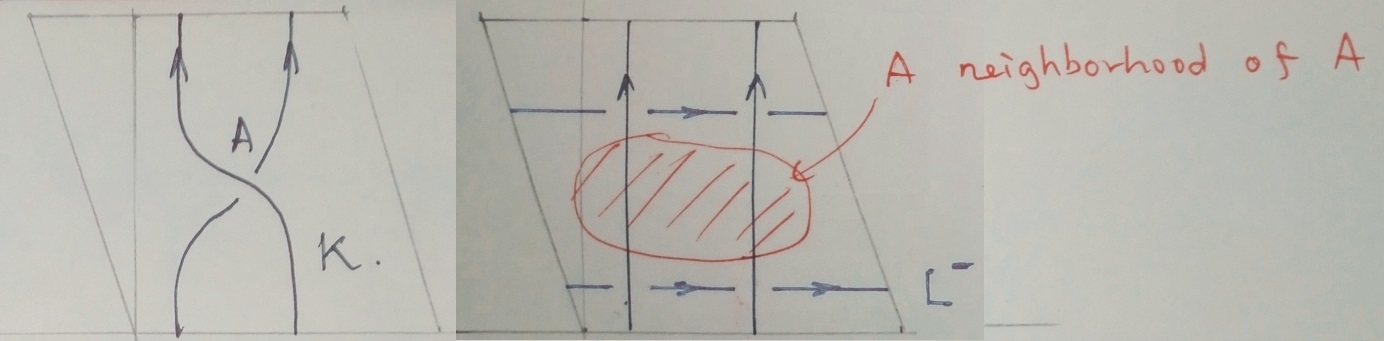
      Figure 2: Here is a knot K in L(3,1), $[L]=2\lambda_{1},r=3,r[L]=2\mu_{1}+2\mu_{2}$. The blue line $L^{-}$ a

      For convenient, $(-(rna+\frac{rnbq}{p})\mu_{1})$ on $\partial V_{1}\times\{1\}$ should be drawn a little bit above the $(rna+\frac{rnbq}{p})\mu_{1}$ on the diagram.

      

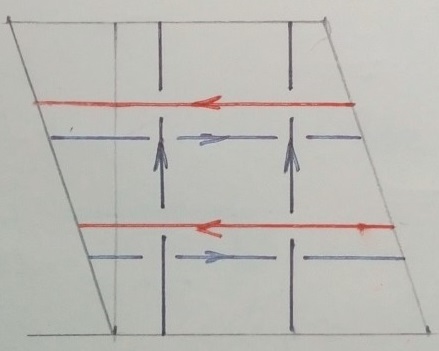
      Figure 3: the red line of homotopy type $(-2\mu_{1})$ is not far away from the blue.

   2. draw torus link $rL$ on $\partial V_{1}\times\{1\}$. Here, $rL$ is r parallel copies of L. For convenience, one shouldn’t draw $rL$ too far away from $L$.

      

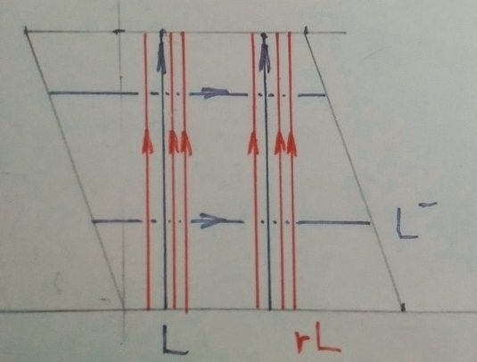
      Figure 4: the red line $rL$ is far from L in the diagram we draw on.

   3. At each intersection of $(-(rna+\frac{rnbq}{p})\mu_{1})$ and $rL$ on $\partial V_{1}\times\{1\}$, replace intersection by smooth arc shown by the graph below.

      

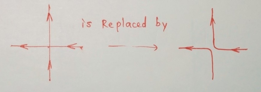
      Figure 5: the other cases it quite similar.

      Then, we get a link $L^{+}$ on $\partial V_{1}\times\{1\}$ with homology class $[L^{+}]=r[L]-(rna+\frac{rnbq}{p})\mu_{1}=\frac{rnb}{p}\mu_{2}$. Therefore, its components is torus knot of $\pm\mu_{2}$ type or null-homologous (simple closed curve on torus). $L^{\prime}$ is the union of $L^{+}$ and $L^{-}$

      

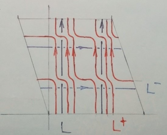
      Figure 6: the black is link $L$, the red is $L^{+}$ and the blue is $L^{-}$

   4. The ”cobordism” of $L$ is actually bounded by $L$ and $L^{\prime}$. Near the intersection of $L$ and $(rna+\frac{rnbq}{p})\mu_{1}$ link on the diagram, the ”cobordism” is glued by the bands below. Outside the neighborhood, the ”cobordism” is obtained by gluing r bands along $L$

      

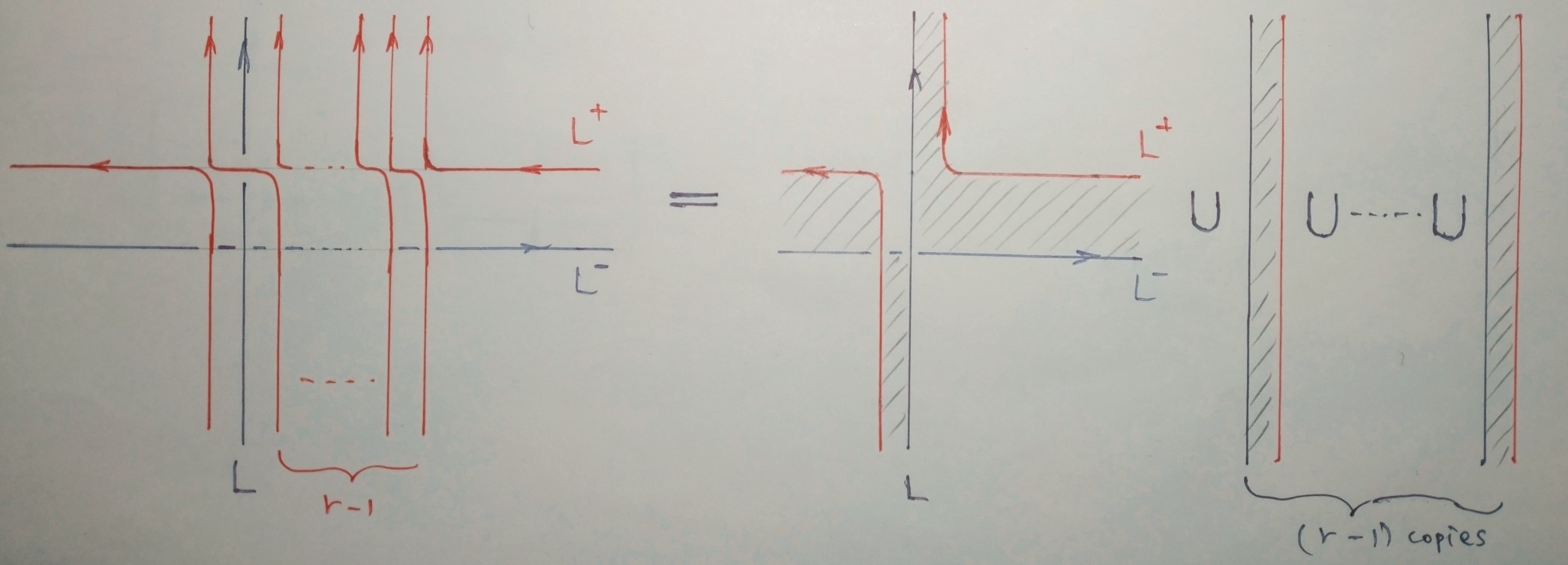
      Figure 7: the other cases are quite similar with this figure

   5. For a very special case when $[L]=0\in H_{1}(\partial V_{1})$, $L^{\prime}=\emptyset$ and $L$ consists of m($m\geq 0$) non-trivial torus knots of type $a\mu_{1}+b\lambda_{1}$, m torus knots of type $-(a\mu_{1}+b\lambda_{1})$ and several null-homologous knots on torus. We construct disjoint m bands (i.e $S^{1}\times I$) and several discs bounded by null-homologous components of $L$

4. Construct r-cover half-twist band as follow. Let $I\times I\times\{1,2,\dots,r\}$ be k-copies of a square. Define equivalent relationship $\sim$ by: $(x,0,1)\sim(x,0,k)$ and $(x,1,1)\sim(x,1,k)$.

   

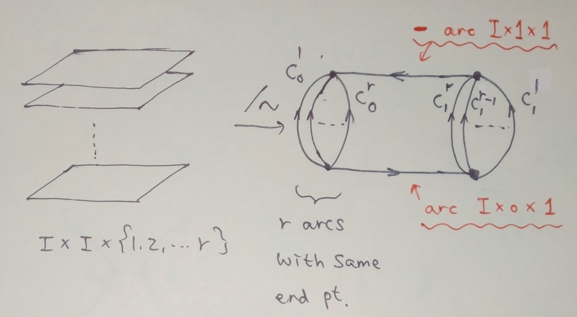
   Figure 8: the other cases are quite similar with this figure

   Then do a half-twist along straight line $I\times\{\frac{1}{2}\}\times\{0\}$ on the quotient space $I\times I\times\{1,2,\dots,r\}/\sim$, the construction of r-cover half-twist band is done. Name arc $\{i\}\times I\times\{k\}$ by $c_{i}^{k}$ where $i=0,1;k=1,2,\dots,r$.

   

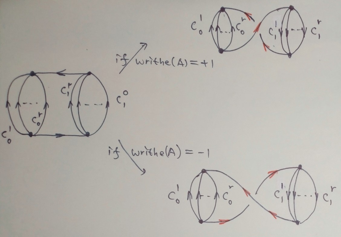
   Figure 9: there are two type of r-cover half-twist band

5. In the first step, we cut apart the crossings (denoted by A) of $P(K)$ into two points $A_{0,1}$.

   

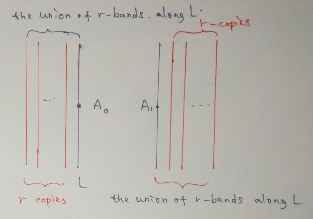
   Figure 10: locally, the cobordism looked like above. Each local component is obtained by gluing r bands along L

   Now we cut off a 3-ball $B_{i}$ of a very small radius centered at each $A_{i=0,1}$ from the ”cobordism” constructed above. The boundary of 3-ball $\partial B_{i}$ intersects the cobordism at r arcs with same endpoints. These arcs is denoted by $\gamma_{i}^{k}$ where $i=0,1;k=1,2,\dots,r$.

   

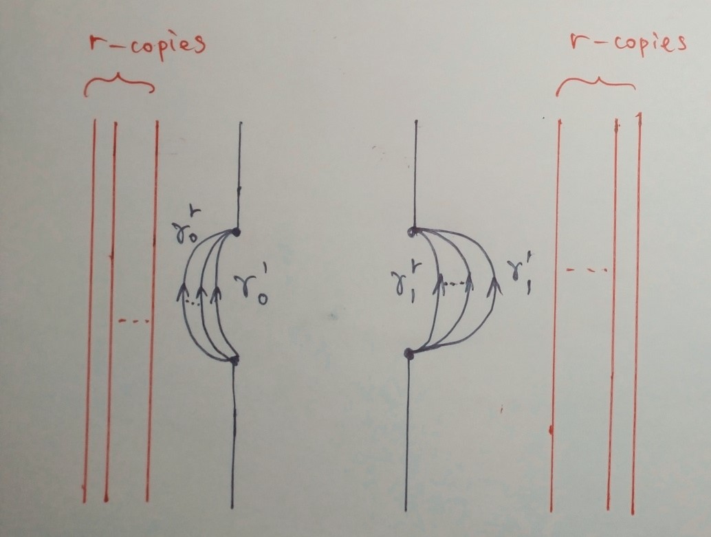
   Figure 11: $\gamma_{i}^{k}$ is marked in the figure

   Now we attach r-cover half-twist band to the punctured cobordism described above by regarding $\gamma_{0}^{k}$ as $c_{0}^{k}$ and $\gamma_{1}^{k}$ as $-c_{1}^{k}$, $k=1,2,\dots,r$. One should take care that the type of r-cover half-twist band to be glued is depended on the writhe of this crossing. Then we get the cobordism from $rK$ to $L^{\prime}$.

6. Now we get the cobordism from $rK$ to $L^{\prime}$. We gluing meridian discs of $V_{1}$ along $L^{-}$, and meridian discs of $V_{2}$ along the $\pm\mu_{2}$-type component of $L^{+}$.For those null-homologous component of $L^{+}$, we glue the discs bounded by them ,probably with a little push off the diagram s.t.the discs are disjoint.

Now we get a rational Seifert surface of $K$. It’s not hard to compute its Eular characteristic. Also, we can find out how it wraps on K. See corollary below

Corollary 1.

Let $K$ be a knot in the interior of $\partial V_{1}\times I$ with homotopy type $[K]=n(a\mu_{1}+b\lambda_{1})$ where $n,a,b\in\mathbf{Z},g.c.d.(a,b)=1$. Let $NK$ be a tubular neighborhood of $K$ with framing $(\mu_{NK},\lambda_{NK})$. Choose the longitude $\lambda_{NK}$ of $NK$ to be the one induced from the push-off of K along the positive direction of $I$. Then, the rational Seifert surface of $K$ intersects $\partial NK$ at a torus link with homology type:

$$r\lambda_{NK}-(rn^{2}(a+\frac{bq}{p})b+rwrithe(K))\mu_{NK}$$

where the writhe of K is the sum of index defined in the graph of the first step1.

Proof.

the proof is not difficult noticing that the construction of cobordism of $L$ devotes

$$-rn^{2}(a+\frac{bq}{p})b\mu_{NK}$$

and the attachment of r-cover half-twist bands devotes

$$-rwrithe(K)\mu_{NK}$$

. ∎

4 Acknowledgement

I would like to thank YouLin Li from SJTU. Without his help, I would not complete this thesis.

References

- [1] Dale Rolfsen. Knots and Links, AMS CHELSEA PUBLISHING, 2000.
- [2] Kenneth Baker and John Etnyre. Rational Linking and Contact Geometry. Perspectives in Analysis, Geometry, and Topology, Progr. Math. 296 (Birkhäuser, Basel, 2012), 19–37.
- [3] Kenneth L. Baker, J. Elisenda Grigsby, and Matthew Hedden. Grid diagrams for lens spaces and combinatorial knot Floer homology. math.GT/0710.0359, 2007.