Integrated correlators from integrability: Maldacena-Wilson line in ${\cal N}=4$ SYM

Abstract

We present a systematic method for the derivation of a relation which connects the correlation function of operators on the straight Maldacena-Wilson line with the integrability data for the cusp anomalous dimension. As we show, the derivation requires very careful treatment of the UV divergences. Our method opens a way to derive infinitely many constraints on integrals of multi-point correlation functions, relating them with the integrability data for the generalised cusp anomalous dimension governed by the Quantum Spectral Curve. Such constraints have been shown recently to be very powerful in combination with the numerical conformal bootstrap, leading to very narrow non-perturbative bounds on conformal data beyond the spectrum.

1 Introduction

Recently, the combination of the exact techniques of integrability and the conformal bootstrap has proven to be very powerful for the non-perturbative study of beyond-the-spectrum observables in higher-dimensional interacting conformal field theories (CFT) such as ${\cal N}=4$ SYM Cavaglia:2021bnz ; Cavaglia:2022qpg ; Caron-Huot:2022sdy . The main idea of this program, called Bootstrability, is to inject non-perturbative spectral information – obtained using a powerful integrability-based method called Quantum Spectral Curve (QSC) Gromov:2013pga ; Gromov:2014caa – into the crossing equations of the CFT of interest. Even without knowing the spectrum, the methods of the numerical conformal bootstrap (NCB) Rattazzi:2008pe ; El-Showk:2012cjh ; Poland:2018epd ; Chester:2019wfx allow one to obtain bounds on various observables (mainly the spectrum but also structure constants), see e.g. for applications to AdS/CFT Agmon:2017xes ; Beem:2013qxa ; Beem:2016wfs ; Chester:2021aun . Especially at strong coupling, those bounds become very narrow allowing for analytic studies too Aharony:2016dwx ; Alday:2017xua ; Alday:2022uxp ; Alday:2022xwz . In combination with the methods of integrability, one can focus more sharply on the structure constants, and obtain extremely narrow bounds on the latter Cavaglia:2021bnz ; Cavaglia:2022qpg , as shown on figure 1, with the leading OPE coefficient determined with the error as small as $10^{-6}$ at the ’t Hooft coupling $\lambda\sim 25$, and the bound rapidly shrinking at stronger and weak coupling.

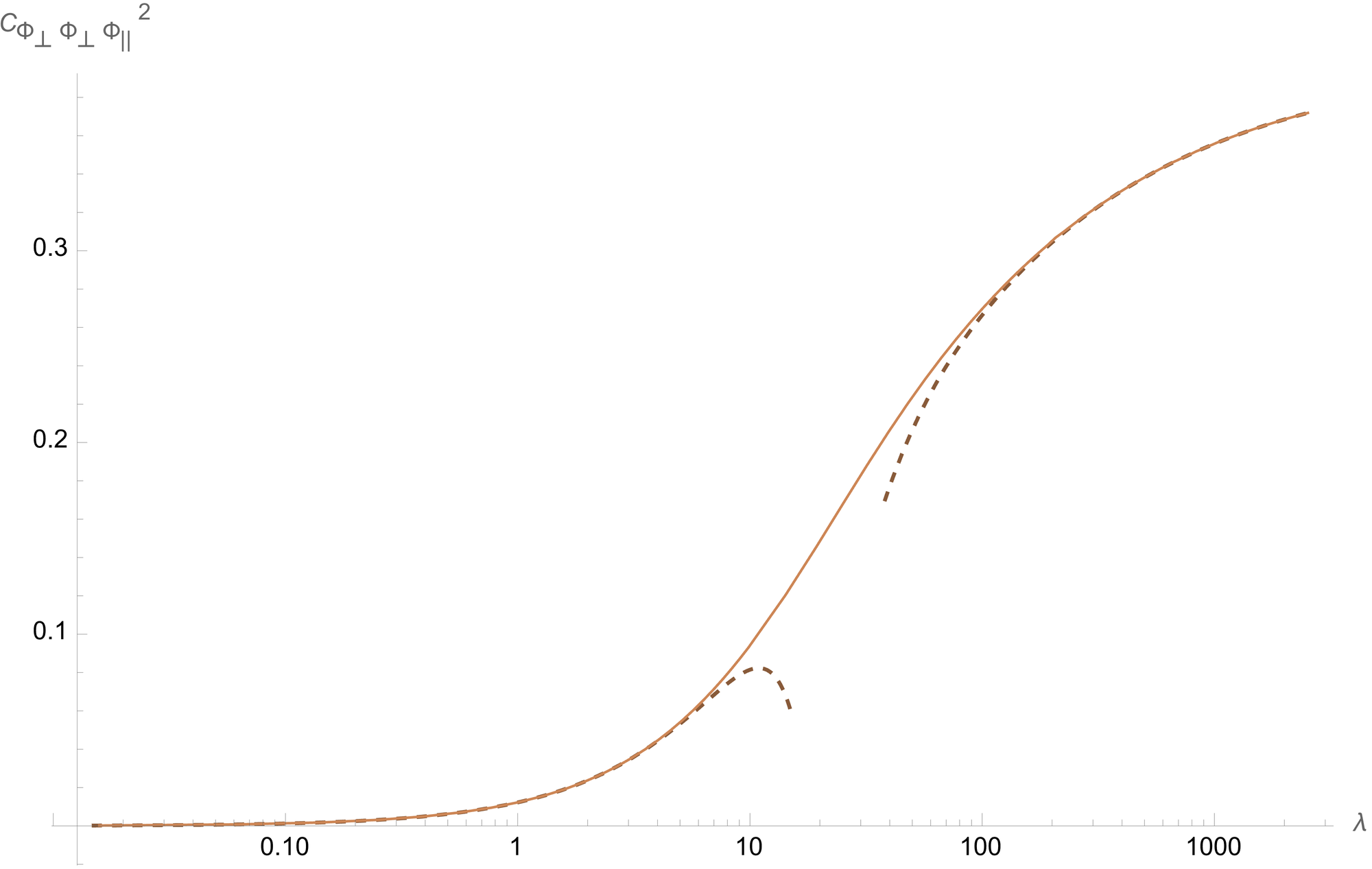
Figure 1: High precision non-perturbative evaluation of the structure constant of two protected one non-protected operators $C^{2}_{\Phi_{\perp}\Phi_{\perp}\Phi_{||}}$ in the defect CFT living on the Maldacena-Wilson line, as obtained by Cavaglia:2022qpg (solid line). Dashed lines represent weak and strong coupling analytic results of Kiryu:2018phb ; Cavaglia:2022qpg ; Ferrero:2021bsb

In particular, in Cavaglia:2022qpg it was realised that, in addition to the spectrum of the CFT itself, one can inject even more spectral data coming from integrable deformations of the setup. In the setup considered here, which we review in detail below, the relevant integrable deformation is that of a supersymmetric straight Maldacena-Wilson line (MWL) deformed by forming a cusp. The extra spectral data pertaining to the anomalous dimension of the cusp impose additional constraints on the conformal data of the defect CFT, on top of the crossing equations. These constraints manifest themselves as extra relations on integrated multi-point functions. Including those in the bootstrap dramatically improves the bounds on the OPE coefficients (shrinking them by $4-5$ orders of magnitude for the leading one, as compared to when the spectrum alone is included! Cavaglia:2022qpg ). Similar relations on the integrated four-point function of four local operators in ${\cal N}=4$ SYM have recently been obtained using localisation, rather than integrability, in Binder:2019jwn ; Paul:2022piq (see also Dorigoni:2021bvj ; Dorigoni:2021guq ; Dorigoni:2022zcr ), and have been shown to also greatly help improving the bounds given by the NCB Chester:2021aun . The advantage of the integrability-generated constraints is that, in principle, they allow one to also constrain correlators with non-BPS external operators. Moreover, in general they are complementary to the information one can obtain from localisation. Hence, there is a good chance that the combination of the two approaches could reinforce results further, even for the case of local operators.

In Cavaglia:2022qpg , we found and already used two such constraints for the correlators of 4 point correlators on top of a MWL. Recently, in Drukker:2022pxk , a specific linear combination of these constraints was derived using general geometric arguments about the structure of the conformal manifold. In this paper, we present a very different argument, which allowed us to derive the remaining independent constraint. As we will show, the derivation requires very careful treatment of the UV divergences and contains many technically involved steps (mostly detailed in the appendices of this paper), but should allow for further generalisations. In particular, one should be able to obtain constraints on 6-point functions, of the type studied recently at weak coupling in Barrat:2021tpn ; Barrat:2022eim .

This paper is organised as follows. In section 2 we describe the setup of the one-dimensional CFT together with its deformations as well as the integral constraints found in Cavaglia:2022qpg in a notation that we will use for our derivation. In section 3 we explain our main strategy and introduce the tools of conformal perturbation theory, as well as describing our regularisation scheme. Finally, in section 4 we present our main result, the derivation of an integrated correlator related to the Curvature function known from integrability. Technical details are collected in the appendices.

2 Setup

In this section we describe in detail our setup. After the definition of supersymmetric Wilson line, we describe the properties of the one-dimensional CFT which lives on top of it. We introduce also the deformations of this CFT and their relation to insertions of local operators and the two crucial quantities – the Bremsstrahlung and Curvature functions. Finally, we review the integrated correlators found initially in Cavaglia:2022qpg .

2.1 The $1/2$ BPS Maldacena-Wilson line

We consider the one dimensional defect created by the supersymmetric Maldacena-Wilson loop (MWL) Maldacena:1998im in 4D $\mathcal{N}=4$ SYM, defined as follows

$${\cal W}_{\mathcal{C}}=\frac{1}{N}\operatorname{Tr}\operatorname{P}\exp\int_{\mathcal{C}}dt\,\left(i\,A_{\mu}\dot{x}(t)^{\mu}+|\dot{x}(t)|\;n\cdot\Phi\right)\;,$$ (1)

where the contour $\mathcal{C}$ is parametrised by $x^{\mu}(t)$. The trace $\operatorname{Tr}$ is taken in the fundamental representation and $\operatorname{P}$ stands for the path-ordering. The coupling to the scalars $\vec{n}$ is a six-dimensional vector with unit norm.

In this paper we consider the case when ${\cal C}$ is a straight line (or a circle). In this case the defect preserves half of the supercharges of the full theory. We also fix $\vec{n}=\{0,0,0,0,0,1\}$ and introduce the notation $\Phi_{||}=\vec{n}\cdot\Phi=\Phi^{6}$, while the remaining $5$ scalars we denote as $\Phi_{\perp}^{M}$ with $M=1,\cdots,5$ (with capital Latin indexes). The full ${\rm SO}(6)$ $R$-symmetry of the parent theory is thus broken to ${\rm SO}(5)$ by the MWL. Similarly, the full superconformal symmetry ${\rm PSU}(2,2|4)$ of $\mathcal{N}=4$ SYM is broken in the presence of the defect to ${\rm OSp}(4^{*}|4)$, where the bosonic subgroups are the ${\rm SO}(3)$ rotations about the loop and the 1D conformal group ${\rm SO}(1,2)$ preserving the line.

Despite the MWLs lying on straight lines and circles preserve the same symmetries and are related by a conformal transformation, their expectation values are different due to a subtle anomaly  Drukker:2000rr . More precisely for the straight line, in some natural conventions, $\langle\mathcal{W}_{\text{line}}\rangle=1$ Drukker:1999zq ; Erickson:2000af ; Zarembo:2002an , at the same time the vev of the circular MWL depends on the coupling constant and at large $N$ that is given by Erickson:2000af ; Drukker:2000rr ; Pestun:2009nn

$$\langle\mathcal{W}_{\text{circle}}\rangle=\frac{1}{2\pi g}I_{1}(4\pi g)\,,$$ (2)

where $g$ is the ’t Hooft coupling $g=\tfrac{\sqrt{\lambda}}{4\pi}$ and $I_{n}(z)$ is the modified Bessel function of the first kind. Apart from this curiosity the circle and the straight line are pretty much the same, but for technical reasons we will be working on the circle most of the time in this paper.

2.2 The defect CFT living on the $1/2$ BPS MWL

The straight MWL (1) can be interpreted as a superconformal one-dimensional defect. The defect theory on top of this defect possesses all the standard properties of a conformal field theory. Its operators are realised by inserting $\mathcal{N}$=4 SYM fields along the Wilson line. Operators arrange in (super)multiplets identified by representations of the symmetry unbroken by the defect, 2- and 3-point functions kinematics is constrained and higher point functions can be constructed by the Operator Product Expansion (OPE). In the following we review these general facts.

The states of the 1D defect CFT.

Operators are organised in superconformal multiplets labelled by four quantum numbers according to the unitary representations of the unbroken ${\rm OSp}(4^{*}|4)$ symmetry Gunaydin:1990ag ; Liendo:2016ymz . The quantum numbers can be represented in the form $\{\Delta,\left[a,b\right],s\}$ where $\Delta$ is the scaling dimension, $\left[a,b\right]$ are the Dynkin labels associated with the $R$-symmetry and $s$ is the spin associated with rotations about the line. At generic values of finite coupling, the 1D CFT admits two classes of supermultiplets. The simplest ones are the $1/2$-BPS short multiplets denoted as ${\cal B}_{k}$, whose superconformal primaries have scaling dimensions protected by supersymmetry with quantum numbers $\{n,\left[0,n\right],0\}$ with $n\in\mathbb{Z}$. In addition to these, the defect theory admits long multiplets ${\cal L}^{\Delta}_{s,\left[a,b\right]}$ which in principle preserve no supercharges. Then, their scaling dimension is not protected by supersymmetry which therefore is a non-trivial function of the coupling $g$.

The CFT multiplets obey OPE selection rules. The one that will be relevant in our setup is the following Liendo:2018ukf

$$\mathcal{B}_{1}\times\mathcal{B}_{1}=\mathcal{I}+\mathcal{B}_{2}+\sum_{\Delta>1}\mathcal{L}_{0,[0,0]}^{\Delta}\;,$$ (3)

where $\mathcal{B}_{1}$ is the multiplet containing $\Phi_{\perp}^{M}$ as we discuss below. The $1/2$-BPS multiplets $\mathcal{B}_{1}$ and $\mathcal{B}_{2}$ were also considered in Giombi:2017cqn ; Liendo:2016ymz ; Cooke:2017qgm ; Liendo:2018ukf ; Ferrero:2021bsb , $\mathcal{I}$ is the identity multiplet and ${\cal L}_{0,\left[0,0\right]}^{\Delta}$ are the non-protected long multiplets transforming as singlets under the global ${\rm SO}(5)\times{\rm SO}(3)$ symmetry.

Operators appearing in the sum of the r.h.s. of (3), such as for example $\Phi_{||},\;\Phi_{||}^{2}$, $(\Phi_{\perp}\cdot\Phi_{\perp}),\;\dots$ mix and develop anomalous dimensions that can be computed using the QSC as shown in Grabner:2020nis ; Cavaglia:2021bnz ; Cavaglia:2022qpg ; Julius:2021uka . By the unitarity bounds, it is known that these non-protected operators are all irrelevant, i.e. with $\Delta>1$ Agmon:2020pde . Importantly, while $\Phi_{\perp}^{M}$ are protected exactly marginal operators with dimension $\Delta=1$, the operator corresponding to $\Phi_{||}$ is an irrelevant operator with a running dimension $\Delta>1$ (except exactly at zero coupling, where $\Delta\rightarrow 1$).

Let us describe the structure of the $\mathcal{B}_{1}$ multiplet in more detail. It is the simplest protected multiplet and it contains three operators with the following quantum numbers

$$\mathcal{B}_{1}:\qquad\{1,\left[0,1\right],0\}\;\longrightarrow\;\{\tfrac{3}{2},\left[1,0\right],\tfrac{1}{2}\}\;\longrightarrow\;\{2,\left[0,0\right],1\}\,,$$ (4)

where arrows represent the action of supercharges on the highest weight. This multiplet is also known as displacement multiplet. Indeed, every defect theory has a distinguished operator called displacement operator, which captures the breaking of translation invariance by the defect. In particular, the stress-energy tensor is no longer conserved and the usual conservation law needs to be modified by some additional terms localised on the defect. In our case it leads to

$$\partial_{\mu}T^{\mu n}=\mathbb{D}^{n}(x_{||})\delta^{3}(x_{\perp})\,,$$ (5)

with $x_{||}=t$ the direction along the defect and $x_{\perp}$ the orthogonal ones. The operator $\mathbb{D}^{n}$ contains the components of the field-strength and it is protected. Given the definition (5), its dimension is 2 and it corresponds to the last operator appearing in the multiplet $\mathcal{B}_{1}$ (4). Also the R-current can be broken giving rise to other operators. These operators have protected dimension 1 and, in our case, they are just the marginal operators $\Phi_{\perp}^{M}$ with $M=1,\dots,5$ corresponding to the highest weight of the supermultiplet $\mathcal{B}_{1}$ (4).

Correlation functions.

Correlation functions are defined as local insertions of operators along the contour as follows Drukker:2006xg

$$\left\langle\left\langle O_{1}\left(t_{1}\right)O_{2}\left(t_{2}\right)\cdots O_{n}\left(t_{n}\right)\right\rangle\right\rangle\equiv\frac{\langle\operatorname{Tr}\operatorname{P}{O}_{1}(t_{1})\,\mathcal{W}_{t_{1},t_{2}}\,{O}_{2}(t_{2})\,\ldots\,O_{n}(t_{n})\,\mathcal{W}_{t_{n},t_{1}}\rangle}{\langle\mathcal{W}_{\mathcal{C}}\rangle}\;,$$ (6)

where $O_{i}$ are composite fields transforming in the adjoint representation of the gauge group and $\mathcal{W}_{t_{a},t_{b}}$ are segment of the Wilson loop $\mathcal{W}_{\mathcal{C}}$ between positions $t_{a}$ and $t_{b}$. The double brackets $\left\langle\left\langle\cdots\right\rangle\right\rangle$ indicate that the vev is taken with the supersymmetric Wilson loop as the vacuum instead of the usual one.

The $n$-point functions (6) satisfy all the properties of a 1D conformal field theory. Then, two- and three-point functions are completely fixed by conformal symmetry. For instance, for scalar operators $O_{\Delta_{i}}$ with dimension $\Delta_{i}$ we have

$$\begin{split}\langle\langle O_{\Delta_{i}}(t_{1})\;O_{\Delta_{j}}(t_{2})\rangle\rangle&=N_{i}\frac{\delta_{ij}}{x_{12}^{2\Delta_{i}}}\equiv N_{i}\delta_{ij}[P(t_{1},t_{2})]^{\Delta_{i}},\\ \langle\langle O_{\Delta_{i}}(t_{1})\;O_{\Delta_{j}}(t_{2})\;O_{\Delta_{k}}(t_{3})\rangle\rangle&=\sqrt{N_{i}N_{j}N_{k}}\frac{C_{ijk}}{x_{12}^{\Delta_{i}+\Delta_{j}-\Delta_{k}}\;x_{23}^{-\Delta_{i}+\Delta_{j}+\Delta_{k}}\;x_{13}^{\Delta_{i}-\Delta_{j}+\Delta_{k}}},\end{split}$$ (7)

with $x_{ab}=|x^{\mu}(t_{a})-x^{\mu}(t_{b})|$ and $C_{ijk}$ the structure constant. We also introduced the function $P(t_{1},t_{2})=\frac{1}{|x(t_{1})-x(t_{2})|^{2}}$ for convenience. We will use the two standard parametrisations: on the line parametrised by $x^{\mu}(t)=\{t,0,0,0\}$, $t\in[-\infty,+\infty]$ and on the unit circle parametrised by $x^{\mu}(t)=\{\cos t,\sin t,0,0\}$, $t\in[0,2\pi]$. So that we have $x_{ab}=|t_{b}-t_{a}|$ on the line and $x_{ab}=\sqrt{2-2\cos(t_{b}-t_{a})}$ for the circle. We assume that by default in the first line of (7) $N_{i}=1$, which is the standard normalisation of the operators. However, for the operators in the displacement multiplet (4) it is more convenient to introduce a non-trivial normalisation as follows

$$\langle\langle\Phi_{\perp}^{M}(t_{1})\Phi_{\perp}^{N}(t_{2})\rangle\rangle=\frac{N_{\Phi_{\perp}}\,\delta^{MN}}{x_{12}^{2}},\qquad\langle\langle\mathbb{D}^{n}(t_{1})\;\mathbb{D}^{m}(t_{2})\rangle\rangle=\frac{N_{\mathbb{D}}\,\delta^{nm}}{x_{12}^{4}},\qquad$$ (8)

where $C_{\Phi_{\perp}}$ and $C_{\mathbb{D}}$ are functions of the coupling as defined below in (38).

Conformal symmetry constrains also 4-point functions. Indeed, in one dimension they can be written in terms of a single cross ratio

$$x=\frac{x_{12}x_{34}}{x_{13}x_{24}}\,,$$ (9)

as follows

$${G}^{MNPQ}(x)\equiv\frac{\langle\langle\Phi_{\perp}^{M}(t_{1})\Phi_{\perp}^{N}(t_{2})\Phi_{\perp}^{P}(t_{3})\Phi_{\perp}^{Q}(t_{4})\rangle\rangle}{P(t_{1},t_{2})P(t_{3},t_{4})}\;,$$ (10)

where $M,N,P,Q=1,\dots,5$. Exploiting the superconformal OPE (3), it is possible to parametrise the 4-point function (10) as

$$G^{MNPQ}(x)=\delta^{MP}\;\delta^{NQ}\;G_{2}(x)+\delta^{MN}\;\delta^{PQ}\;G_{1}(x)+\delta^{MQ}\;\delta^{NP}\;G_{3}(x)\,,$$ (11)

with

$$\begin{split}G_{1}(x)&=(x-1)f^{\prime}(x)+\left(\frac{2}{x}-1\right)f(x)\,,\\ G_{2}(x)&=\mathbb{F}\;x^{2}-(x-1)xf^{\prime}(x)-f(x)\,,\\ G_{3}(x)&=f(x)-xf^{\prime}(x)\,,\end{split}$$ (12)

and, in case of identical protected operators polarised in the same direction i.e. $M=N=P=Q$ as

$$\begin{split}{G}(x)&=G_{1}(x)+G_{2}(x)+G_{3}(x)\\ &=\mathbb{F}\;x^{2}+(2x^{-1}-1)f(x)-\left(x^{2}-x+1\right)f^{\prime}(x)\;,\end{split}$$ (13)

where the reduced correlator $f(x)$ appearing in (12) and (13) is a function of the cross ratio containing the OPE decomposition

$$f(x)=F_{\mathcal{I}}(x)+{{C^{2}_{\rm BPS}\,{F}_{\mathcal{B}_{2}}(x)}}+\sum_{n}{{C^{2}_{n}\,{F}_{{\Delta_{n}}}(x)}}\;,$$ (14)

with superconformal blocks given by

$$F_{\mathcal{I}}(x) = x\;,$$ (15)

$$F_{\mathcal{B}_{2}}(x) = x-x\,_{2}F_{1}(1,2,4;x)\;,$$ (16)

$$F_{{\Delta}}(x) = \frac{x^{\Delta+1}}{1-\Delta}\,_{2}F_{1}(\Delta+1,\Delta+2,2\Delta+4;x)\;,$$ (17)

and OPE coefficients

$$C_{n}\equiv C_{\Phi_{\perp}^{i},\;\Phi_{\perp}^{i},\;\mathcal{L}_{0,[0,0]}^{\Delta_{n}}}\,,$$ (18)

for the non-protected states. Several orders of the reduced correlator are known in perturbation theory, at strong coupling in Ferrero:2021bsb and at weak coupling in Kiryu:2018phb ; Cavaglia:2022qpg .

The constant $\mathbb{F}$ appearing in (14) and the structure constant corresponding to the $\mathcal{B}_{2}$ block are related as $\mathbb{F}(g)=1+C^{2}_{BPS}(g)$. They can be computed exactly both using supersymmetric localisation Giombi:2017cqn ; Liendo:2018ukf or, alternatively, by making contact with integrability with arguments similar to those of this paper, see Cavaglia:2022qpg . The result is

$$\begin{split}\mathbb{F}(g)=1+C^{2}_{BPS}(g)&=\frac{3\;\langle\mathcal{W}_{\text{circle}}\rangle\;\langle\mathcal{W}_{\text{circle}}\rangle^{\prime\prime}}{(\langle\mathcal{W}_{\text{circle}}\rangle^{\prime})^{2}}\\ &=\frac{3I_{1}(4g\pi)\left(\left(2\pi^{2}g^{2}+1\right)I_{1}(4g\pi)-2g\pi I_{0}(4g\pi)\right)}{2g^{2}\pi^{2}I_{2}(4g\pi){}^{2}}\;\;,\end{split}$$ (19)

where the first expression refers to the expectation value of the circular Wilson loop given in (2).

Finally, given the invariance under the cyclic relabelling of the 4-point function (10), the quantities $G(x)$ and $f(x)$ satisfy the following crossing equations

$$\begin{split}x^{2}{G}(1-x)-(1-x)^{2}{G}(x)&=0\,,\\ x^{2}f(1-x)+(1-x)^{2}f(x)&=0\;.\end{split}$$ (20)

The main goal of this paper is to relate the deformation of this CFT with the integrability data. We discuss the deformations in the next section.

2.3 The defect deformations

The displacement deformations.

The Ward identity (5) fixes the variation of an arbitrary correlation function when the contour of the defect undergoes a small deformation. Let us consider the deformation of a linear defect parametrised by $x_{||}=t$ by a profile $\delta x_{\perp}^{n}(t)$. Then, the correlation function $\langle\langle O\rangle\rangle$ of an arbitrary operator $O$ taken in presence of the deformed Wilson loop, at first order in the deformation reads Polyakov:2000ti ; Semenoff:2004qr ; Correa:2012at

$$\langle\langle\,O\,\rangle\rangle_{x+\delta x}=\int dt\;\langle\langle\,O\;\mathbb{D}^{n}(t)\,\rangle\rangle\;\delta x_{\perp}^{n}(t)+\mathcal{O}(\delta x^{2})\,,$$ (21)

where we assume that $\delta x(t)$ vanishes at the locations of the operators $O$. Similarly for the vev of the Wilson loop itself, with the difference that the first order variation vanishes since it corresponds to a one-point function on the defect CFT. The first non-trivial contribution appears at second order in the deformation and it is given by

$$\delta_{x}\log\langle\,\mathcal{W}_{\mathcal{C}}\,\rangle=\int_{t_{1}>t_{2}}dt_{1}dt_{2}\;\langle\langle\,\mathbb{D}^{n}(t_{1})\;\mathbb{D}^{m}(t_{2})\,\rangle\rangle\;\delta x_{\perp}^{n}(t_{1})\delta x_{\perp}^{m}(t_{2})+\mathcal{O}(\delta x_{\perp}^{3})\;.$$ (22)

For the supersymmetric Wilson loop (1) there is also an internal angle displacement operator corresponding to $\Phi_{\perp}^{N}$, $N=1,\dots,5$, the highest weights of the displacement multiplet. These operators are sometimes referred to as tilt operators. One can see these operators arising when the coupling to the scalars in the Wilson loop connection (1) is deformed as $n+\delta n$, with $n\cdot\delta n=0$, leading to

$$\delta_{n}\log\langle\,\mathcal{W}_{\mathcal{C}}\,\rangle=\int_{t_{1}>t_{2}}dt_{1}dt_{2}\;\langle\langle\,\Phi_{\perp}^{N}(t_{1})\;\Phi_{\perp}^{M}(t_{2})\,\rangle\rangle\;\delta n^{N}(t_{1})\delta n^{M}(t_{2})+\mathcal{O}(\delta n^{3})\;.$$ (23)

Integrability data for the WL deformations.

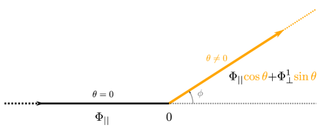
Figure 2: The WL deformed by introducing a point-like parameter changing defect is integrable. We utilise this fact to deduce further constraints on the correlation functions of the 1D CFT on the straight line.

A particular deformation of the defect CFT is given by introducing a cusp along the contour as in figure 2, which can be considered as a point-like parameter changing defect inside WL or also as a particular case of a colour-twist operator introduced in Cavaglia:2020hdb . The resulting operator is composed of two semi-infinite lines connecting in the origin as follows

$${\cal W}_{\text{cusp}}=\frac{1}{N}\operatorname{Tr}\left[W_{-\infty}^{0}(0,0)W_{0}^{+\infty}(\phi,\theta)\right]\;,$$ (24)

where the second infinite segment is rotated both in space-time with angle $\phi$ forming the cusp, as well as in the space of scalar couplings with the internal angle $\theta$. Choosing planes for the rotations, the two rays can be written as follows

$${W}_{t_{1}}^{t_{2}}(\phi,\theta)=\operatorname{P}\exp\int_{t_{1}}^{t_{2}}dt\bigg{[}i\,A_{\mu}\dot{x}^{\mu}(t)+(\Phi_{||}\cos\theta+\Phi^{1}_{\perp}\sin\theta)\,|\dot{x}(t)|\bigg{]}\;,$$ (25)

with the contour parametrised by $x(t)=\big{(}t\cos\phi,t\sin\phi,0,0\big{)}$.

The cusped Wilson line is no longer finite and it develops an anomalous dimension known as cusp anomalous dimension. This quantity is defined through the divergence of the vev of $\mathcal{W}_{\text{cusp}}$ as follows Korchemsky:1985xj

$$\langle\,{\cal W}_{\text{cusp}}\,\rangle\sim\left(\epsilon_{\rm UV}\right)^{\Gamma_{\text{cusp}}(g,\phi,\theta)}\;,$$ (26)

where $\epsilon_{\rm{UV}}$ is the UV cutoff near the cusp. Perhaps more transparent way of defining the cusp anomalous dimension, is by mapping the two lines to two intercepting arches of circles, meeting at the external angle $\phi$ as on figure 3. The two arches has two interception points (one is the image of $0$ another is the image of $\infty$), then the expectation value will scale as the distance between these two intersection points (in 4D) to the power $-2\Gamma_{\text{cusp}}(g,\phi,\theta)$.

The cusp anomalous dimension $\Gamma_{\text{cusp}}(g,\phi,\theta)$ was introduced and studied at weak and strong coupling in Drukker:2011za . Moreover, since the configuration introduced in (24) was discovered to be integrable, a set of TBA equations for it was introduced in Correa:2012hh ; Drukker:2012de and reformulated in terms of the QSC in Gromov:2015dfa allowing for its non-perturbative analysis.

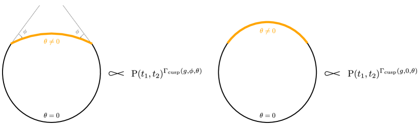
Figure 3: Another conformally equivalent representation of the cusped WL. The expectation value of this object depends on the distance between the cusps in the standard way as a two point function of two operators of dimension $\Gamma_{\rm cusp}$.

In the near-BPS limit $\phi\to\pm\theta$, the first few orders of the cusp anomalous dimension are given by

$$\Gamma_{\text{cusp}}(g,\phi,\theta)=\frac{\cos\phi-\cos\theta}{\sin\phi}\frac{2\phi}{1-\frac{\phi^{2}}{\pi^{2}}}\mathbb{B}(g,\phi)+\left(\frac{\cos\phi-\cos\theta}{\sin\phi}\right)^{2}\phi^{2}\mathbb{C}(g,\phi)+...\;,$$ (27)

where the dots represents higher orders in $\tfrac{\cos\phi-\cos\theta}{\sin\phi}$. The function $\mathbb{B}(g,\phi)$ is known as Bremsstrahlung function originally computed in Correa:2012at ; Fiol:2012sg exploiting the supersymmetric localisation techniques Erickson:2000af ; Drukker:2000rr ; Drukker:2006ga ; Pestun:2009nn . The same result was later reproduced and further generalised from integrability in Gromov:2012eu ; Gromov:2013qga and checked at strong and weak coupling in Sizov:2013joa ; Bonini:2015fng . The function $\mathbb{C}(g,\phi)$ appearing in (27) was computed analytically in Gromov:2015dfa using the QSC formalism. We will refer to it as Curvature function.

For what follows it is useful to consider the cusp anomalous dimension in the case in which the Euclidean angle $\phi$ is set to zero and $\theta$ is small. This corresponds to study a small deformation of the $1/2$-BPS Wilson line, leading to the following expansion

$$\Gamma_{\text{cusp}}(g,\phi=0,\theta\rightarrow 0)=\mathbb{B}(g)\,\sin^{2}\theta+\frac{1}{4}\left(\mathbb{B}(g)+\mathbb{C}(g)\right)\,\sin^{4}\theta+\mathcal{O}(\sin^{6}\theta)\;.$$ (28)

Finally, let us write the expression for the Bremsstrahlung and Curvature functions

$$\mathbb{B}(g) =\frac{g}{\pi}\frac{I_{2}(4\pi g)}{I_{1}(4\pi g)}\;,$$ (29)

$$\mathbb{C}(g) =-4\,\mathbb{B}^{2}(g)-\frac{1}{2}\oint\frac{du_{x}}{2\pi i}\oint\frac{du_{y}}{2\pi i}K_{0}(u_{x}-u_{y})F[x,y]\;,$$ (30)

where we use the shorthand notation $\mathbb{B}(g,\phi=0)\equiv\mathbb{B}(g)$ and $\mathbb{C}(g,\phi=0)\equiv\mathbb{C}(g)$. Here both integrals run clockwise around the cut $[-2g,2g]$ and $u_{x}=g(x+1/x)$ is the Zhukovsky parametrisation. The kernel $K_{0}$ and the integrand $F$ are given in appendix A.

Curiously, the function $\mathbb{F}$, appeared in the correlator (19) could be written in terms of the $\mathbb{B}$ as follows

$$\mathbb{F}(g)=\frac{3(g^{2}-\mathbb{B}(g))}{\pi^{2}\mathbb{B}(g)^{2}}\;\;.$$ (31)

The integral (30) was solved perturbatively in Cavaglia:2022qpg . At weak coupling it gives

$$\begin{split}\mathbb{C}&=4g^{4}-\left(24\zeta_{3}+\frac{16\pi^{2}}{3}\right)g^{6}+\left(\frac{64\pi^{2}\zeta_{3}}{3}+360\zeta_{5}+\frac{64\pi^{4}}{9}\right)g^{8}\\ &-\left(\frac{112\pi^{4}\zeta_{3}}{5}+272\pi^{2}\zeta_{5}+4816\zeta_{7}+\frac{416\pi^{6}}{45}\right)g^{10}\\ &+\left(\frac{3488\pi^{6}\zeta_{3}}{135}+\frac{2192\pi^{4}\zeta_{5}}{9}+\frac{9184\pi^{2}\zeta_{7}}{3}+63504\zeta_{9}+\frac{176\pi^{8}}{15}\right)g^{12}+\mathcal{O}\left(g^{14}\right)\;.\end{split}$$ (32)

At strong coupling, the coefficients of the series in $g$ were deduced by evaluating the integral with very high numerical precision and then fitting with Riemann zeta values $\zeta_{n}$ obtaining the following expansion

$$\begin{split}\mathbb{C}&=\frac{\left(2\pi^{2}-3\right)g}{6\pi^{3}}+\frac{-24\zeta_{3}+5-4\pi^{2}}{32\pi^{4}}+\frac{11+2\pi^{2}}{256\pi^{5}g}+\frac{96\zeta_{3}+75+8\pi^{2}}{4096\pi^{6}g^{2}}\\ &+\frac{3\left(408\zeta_{3}-240\zeta_{5}+213+14\pi^{2}\right)}{65536\pi^{7}g^{3}}+\frac{3\left(315\zeta_{3}-240\zeta_{5}+149+6\pi^{2}\right)}{65536\pi^{8}g^{4}}+\mathcal{O}\left(\frac{1}{g^{5}}\right)\;.\end{split}$$ (33)

for the next $3$ coefficients we were only able to find their numerical values

$$\frac{3.044012903724157826\times 10^{-7}}{g^{5}}+\frac{8.008516278599531\times 10^{-8}}{g^{6}}+\frac{2.125834835083\times 10^{-8}}{g^{7}}$$

In the ancillary file of this paper, we included the Mathematica notebook Curvature.nb containing the implementation we used to numerically compute the curvature function with high precision.

From cusp anomalous dimension to two-point function.

Let us relate the following two quantities: the normalisation of the two-point function of the deformation operators, and the cusp anomalous dimension at the leading non-trivial order in the deformation parameter following Correa:2012at . The rest of the paper will be dedicated to generalising this consideration to the higher order in the deformation parameter, so this example, while simple, is very useful to demonstrate the general idea. Consider, first, the deformation by $\theta$ while keeping $\phi=0$. We introduce non-zero $\theta$ in the interval $[-T/2,T/2]$, which can be interpreted as a two-point function of two defects and thus we should have

$$\mathcal{W}_{\mathcal{C}}\simeq(T/\epsilon)^{-2\Gamma_{\rm cusp}}\simeq 1-2\theta^{2}{\mathbb{B}}\log\frac{T}{\epsilon},$$ (34)

where $\epsilon$ is a UV cut-off and we used that from (27) $\Gamma_{\rm cusp}=\theta^{2}{\mathbb{B}}$ . Our starting point is (23) with $\delta n(t)=(0,0,0,0,\theta,0)$ for $t\in[-T/2,T/2]$ and zero otherwise

$$\delta_{x}\log\langle\,\mathcal{W}_{\mathcal{C}}\,\rangle=\int_{-T/2}^{T/2-\epsilon}dt_{1}\int_{t_{1}+\epsilon}^{T/2}dt_{2}\;\frac{N_{\Phi_{\perp}}}{(t_{1}-t_{2})^{2}}\;\theta^{2}+{\cal O}(\theta^{3})\;.$$ (35)

Above we introduced the UV cut-offs $\epsilon$. The integration can be evaluated exactly

$$\delta_{x}\log\langle\,\mathcal{W}_{\mathcal{C}}\,\rangle=\left(\frac{T}{\epsilon}-\log\frac{T}{\epsilon}-1\right)C_{\Phi_{\perp}}\theta^{2}\,.$$ (36)

In the section 4 we will introduce a more precise treatment of the linear divergence, but for now we can just drop it and comparing the $\log$ terms with (34) to obtain $N_{\Phi_{\perp}}=2{\mathbb{B}}$.

Similarly, we can analyse the deformation by $\phi$. The small deformation by $\phi$ is equivalent to introducing a tiny bump in the line between $(-T/2,T/2)$, which can be written at the linear order as a parabolic deformation $\delta x(t)=\frac{\phi}{T}\left(\frac{T^{2}}{4}-t^{2}\right)$, approximating a tiny arc of a circle inclusion. One can check that indeed the slope of this line at $t=\pm T$ is $\pm\phi$. From (22) we get

$$\delta_{x}\log\langle\,\mathcal{W}_{\mathcal{C}}\,\rangle=\int_{-T/2}^{T/2-\epsilon}dt_{1}\int_{t_{1}+\epsilon}^{T/2}dt_{2}\;\frac{N_{\mathbb{D}}}{(t_{1}-t_{2})^{4}}\delta x(t_{1})\delta x(t_{2})+{\cal O}(\phi^{3})\;,$$ (37)

the log-divergent part of the integral is $\frac{1}{6}C_{\mathbb{D}}\phi^{2}\log\frac{T}{\epsilon}$ again comparing with $\Gamma_{\rm cusp}=-\phi^{2}{\mathbb{B}}$, as follows from (27) we get $N_{\mathbb{D}}=12\mathbb{B}(g)$. To summarise we get the following normalisations of the 2-point functions

$$N_{\mathbb{D}}=12\mathbb{B}(g)\qquad\text{and}\qquad N_{\Phi_{\perp}}=2\mathbb{B}(g)\;.$$ (38)

Next, we remind the form of the integrated correlators initially found in Cavaglia:2022qpg with the goal to derive a combination of them in the rest of the paper.

2.4 Integrated correlators

In the previous section we discussed how the deformation of the line by a cusp at the leading order produces a normalisation of the two point function. Already at the next order we get a nontrivial relation which involves an integrated four-point function. We will consider the simplest four-point function of four identical protected operators $\Phi_{\perp}^{N}$ introduced in (10), which will be related to the R-symmetry deformation of the Wilson loop operator at next-to-leading order (28). At this order, one can write the following independent constraints Cavaglia:2022qpg , expressed in terms of the reduced correlator $f(x)$ defined in (14),

Constraint 1: $$\int_{\delta_{x}}^{1}\delta f(x)\left(\frac{1}{x}+\frac{1}{x^{3}}\right)dx-\frac{1}{2}(\mathbb{F}-3)\log{\delta_{x}}-\mathbb{F}+3=\frac{3\mathbb{C}-\mathbb{B}}{8\;\mathbb{B}^{2}}\;,$$ (39)

Constraint 2: $$\int_{0}^{1}\frac{\delta f(x)}{x}dx=\frac{\mathbb{C}}{4\;\mathbb{B}^{2}}+\mathbb{F}-3\;,$$ (40)

where $\delta_{x}\rightarrow 0^{+}$ is a cut-off regulator and $\delta f(x)\equiv f(x)-f_{\text{tree}}(x)$ with $f_{\text{tree}}$ the zero-coupling value

$$f_{\text{tree}}(x)=2x+\frac{x}{x-1}\;.$$ (41)

Notice that the expression in the l.h.s. of (39) is finite since $\delta f(x)\sim\frac{3-\mathbb{F}}{2}x^{2}$ for $x\rightarrow 0$. The Bremsstrahlung ${\mathbb{B}}$ and Curvature functions ${\mathbb{C}}$ are defined in (29) and (30).

For completeness, it is worth mentioning that one of the integrals appearing in (39) and (40) can be further simplified by

$$\int_{0}^{1}\frac{\delta f(x)}{x}\,dx=\int_{0}^{1}\delta f(x)\,dx\,,$$ (42)

as follows immediately from the crossing relation (20), which implies that $f(x)(1-1/x)$ is an odd function under crossing and thus vanishes under the integral.

Exploiting the relation between the 4-point function $G(x)$ and the reduced correlator $f(x)$ given in (13), the first integrated constraint (39) can also be written as follows

$$\text{ Constraint 1: }\int_{0}^{1}\delta G(x)\frac{1+\log x}{x^{2}}dx=\frac{3\mathbb{C}-\mathbb{B}}{8\;\mathbb{B}^{2}}\;,$$ (43)

where $\delta G(x)\equiv G(x)-G_{\text{tree}}(x)$ and $G_{\text{tree}}$ is the zero-coupling value:

$$G_{\text{tree}}(x)=\frac{2(x-1)x+1}{(x-1)^{2}}\;.$$ (44)

The integral relations (39) and (40) were tested for several orders at weak and strong coupling in Cavaglia:2022qpg . Recently, the authors of Drukker:2022pxk managed to derive a linear combination of these constraints by using a general argument on the geometry of the conformal manifold. The combination derived in Drukker:2022pxk can be written as

$$-2\int_{\delta_{x}}^{1}\delta f(x)\left(\frac{1}{x}+\frac{1}{x^{3}}\right)dx+(\mathbb{F}-3)\log{\delta_{x}}+3\int_{0}^{1}\frac{\delta f(x)}{x}dx=\frac{1}{4\mathbb{B}}+\mathbb{F}-3\,,$$ (45)

and is independent from the Curvature function. In Drukker:2022pxk it was derived by studying the Riemann tensor of the defect conformal manifold generated by the marginal operator $\Phi_{\perp}$. The aim of this paper is to provide the proof of the other independent linear combination of the constraints.

3 Strategy and Technicalities

In this section we describe the main strategy of our derivation, and then proceed to describe in detail the conformal perturbation theory setup we use for the calculation. The most technical parts of the derivation will be described in the next section.

3.1 The main strategy

Our main goal is relating the cusp anomalous dimension to the integrated correlator of the four scalar operators $\Phi_{\perp}$. The latter, as has been already discussed, are the “tilt operators” controlling deformations of the internal angle along the MWL. Therefore, we will consider the “cusp” defined purely in R-space, i.e. we only consider the deformation by the angle $\theta$ in the notation of Section 2.3. In this case, $\Gamma_{\text{cusp}}$ can be viewed as a scaling dimension of two point-like parameter-changing defects, see the right panel of Figure 3. Namely, we consider a straight (or circular) MWL, where the polarisation of the scalars is modified in an interval between points $t_{1}$ and $t_{2}$. This configuration has an expectation value of the form:

$${\cal W}(t_{1},t_{2};\theta)\equiv\frac{\langle W_{-\infty}^{t_{1}}(0,0)\,W_{t_{1}}^{t_{2}}(0,\theta)\,W_{t_{2}}^{\infty}(0,0)\rangle}{\langle W_{-\infty}^{\infty}(0,0)\rangle}\propto\left(\epsilon_{\text{UV}}^{2}/x_{12}^{2}\right)^{\Gamma_{\text{cusp}}(0,\theta)},$$ (46)

where $\epsilon_{\text{UV}}$ is a UV cutoff controlling the neighbourhood of the points $t_{1}$ and $t_{2}$, as we discussed around (26). This formula follows from the definition of $\Gamma_{\text{cusp}}$ and conformal invariance in the SYM theory, see e.g. Cavaglia:2018lxi ; Dorn:2020meb .

The above expression is written in terms of quantities in $\mathcal{N}$=4 SYM. Our first goal is to rewrite the small $\theta$ expansion of this observable in terms of internal quantities of the 1D defect CFT living on the straight Wilson line. We first explain the main intuition in a treatment suitable at weak coupling, and later we will explain the proper CFT setup suitable to keep the ’t Hooft coupling finite.

3.1.1 From deformations of the MWL to integrated correlators

It is a general expectation that deformations of a Wilson line can be realised in terms of a series of integrated operator insertions on the undeformed contour Drukker:2006xg ; Cooke:2017qgm .

In our case, this can be seen easily from the definition (25), which we repeat here for convenience in the case $\phi=0$ and assuming a straight MWL along the direction $4$ in spacetime

$${W}_{t_{1}}^{t_{2}}(0,\theta)=\operatorname{P}\exp\int_{t_{1}}^{t_{2}}dt\bigg{[}i\,A_{4}(t)+(\Phi_{||}(t)\cos\theta+\Phi^{1}_{\perp}(t)\sin\theta)\bigg{]}\;.$$ (47)

Considering $\mathbf{s}\equiv\sin\theta$ a small expansion parameter, expanding (47) up to the ${\bf s}^{4}$ we find

$${W}_{t_{1}}^{t_{2}}(0,\theta) \sim \operatorname{P}e^{\int_{t_{1}}^{t_{2}}dt\left(i\,A_{3}(t)+\Phi_{||}(t)\right)}\times\exp\int_{t_{1}}^{t_{2}}dt\;\delta L\;\;,$$ (48)

$$\text{with}\quad\delta L = \bigg{[}\mathbf{s}\;\Phi_{\perp}^{1}(t)-\frac{\mathbf{s}^{2}}{2}\;\Phi_{||}(t)-\frac{\mathbf{s}^{4}}{8}\;\Phi_{||}(t)+\dots\bigg{]}\,.$$

We found that in order to get a finite result we have to add divergent counter-terms given by insertions of the identity operator. So, in practice we should use

$$\delta L = \bigg{[}\mathbf{s}\;\Phi_{\perp}^{1}(t)+\mathbf{s}^{2}\left(\frac{b_{2}}{\epsilon}-\frac{1}{2}\;\Phi_{||}(t)\right)+\mathbf{s}^{4}\left(\frac{b_{4}}{\epsilon}-\frac{1}{8}\;\Phi_{||}(t)\right)+{\cal O}({\bf s}^{6})\bigg{]}\,,$$

where $\epsilon$ is the UV regularisation, which will be described in detail in the next section.

For the left hand side of (46) we get

$${\cal W}(t_{1},t_{2};\theta)\sim 1+\mathbf{s}^{2}{\Big{[}}\int\limits_{t_{1}<s_{1}<s_{2}<t_{2}}ds_{1}\,ds_{2}\,\langle\langle\Phi_{\perp}^{1}(s_{1})\Phi_{\perp}^{1}(s_{2})\rangle\rangle+\frac{b_{2}}{\epsilon}\int_{t_{1}}^{t_{2}}ds_{1}\langle\langle\mathds{1}(s_{1})\rangle\rangle{\Big{]}}$$

$$+\frac{\mathbf{s}^{4}}{4}\,{\Big{[}}\!\!\!\!\int\limits_{t_{1}<s_{1}<s_{2}<t_{2}}\!\!\!\!\!\!\!\!\!\!\!ds_{1}\,ds_{2}\,\langle\langle\Phi_{||}(s_{1})\Phi_{||}(s_{2})\rangle\rangle+\frac{4b_{4}}{\epsilon}\!\!\!\!\int\limits_{t_{1}<s<t_{2}}\!\!\!\!\!\!\!ds{\langle\langle\mathds{1}(s)\rangle\rangle}+\frac{4b_{2}^{2}}{\epsilon^{2}}\!\!\!\!\int\limits_{t_{1}<s_{1}<s_{2}<t_{2}}\!\!\!\!\!\!\!\!\!\!\!ds_{1}ds_{2}\,\langle\langle\mathds{1}(s_{1})\mathds{1}(s_{2})\rangle\rangle{\Big{]}}$$

$$-\frac{\mathbf{s}^{4}}{2}\int\limits_{t_{1}<s_{1}<s_{2}<s_{3}<t_{2}}ds_{1}\,ds_{2}\,ds_{3}\left(\langle\langle\Phi_{||}(s_{1})\Phi_{\perp}^{1}(s_{2})\Phi_{\perp}^{1}(s_{3})\rangle\rangle+\texttt{cyclic}\right)$$ (49)

$$+\frac{b_{2}\mathbf{s}^{4}}{\epsilon}\int\limits_{t_{1}<s_{1}<s_{2}<s_{3}<t_{2}}ds_{1}\,ds_{2}\,ds_{3}\left(\langle\langle\mathds{1}(s_{1})\Phi_{\perp}^{1}(s_{2})\Phi_{\perp}^{1}(s_{3})\rangle\rangle+\texttt{cyclic}\right)$$

$$+\mathbf{s}^{4}\,\int\limits_{t_{1}<s_{1}<s_{2}<s_{3}<s_{4}<t_{2}}ds_{1}\,ds_{2}\,ds_{3}\,ds_{4}\,\langle\langle\Phi_{\perp}^{1}(s_{1})\Phi_{\perp}^{1}(s_{2})\Phi_{\perp}^{1}(s_{3})\Phi_{\perp}^{1}(s_{4})\rangle\rangle+{\cal O}\left(\mathbf{s}^{6}\right)\,,$$

where we have already set to zero all correlators appearing in the expansion which vanish for R-symmetry reasons.

As reviewed in section 2.4, the order $\mathcal{O}(\mathbf{s}^{2})$ of this equation, compared with the expansion of $\Gamma_{\text{cusp}}$, fixes the normalisation of the 2-point function of $\Phi_{\perp}^{N}$ in terms of the Bremsstrahlung function $\mathbb{B}$, defined in (28). At the $\mathcal{O}(\mathbf{s}^{4})$ order the last term gives an integrated 4-point function, which by comparing with the r.h.s. of (46) should be related to the curvature function ${\mathbb{C}}$.

Going to higher orders requires to be consistent and careful about regularisation, see e.g. Cooke:2017qgm for studies at weak coupling. In order to deal with the regularisation scheme consistently at finite coupling, in the next section we describe a more abstract formalism of conformal perturbation theory.

3.1.2 Conformal perturbation theory framework

In this section we describe a more abstract point of view about the deformation by the angle $\theta$, using exclusively the 1D CFT language rather than referring to fields in $\mathcal{N}$=4 SYM.

Namely, we view the ${\bf s}=\sin\theta$-deformation as a deformation (locally) by a marginal operator $\Phi_{\perp}^{1}$ at the leading order, which is also accompanied with a perturbation by relevant (such as the identity $\mathds{1}$) and irrelevant (such as $\Phi_{||}$ and possibly others) operators at higher orders. We then constrain the way the irrelevant operators appear by requiring that the deformation is a symmetry or rotation in R-space when extended to the whole line. As at the higher orders in the deformation parameter the regularisation has to be applied consistently, we also give in this section the detailed description of our regularisation scheme. Our consideration follows closely the general conformal perturbation theory framework (see e.g. Cardy:1996xt ; Zamolodchikov:1987ti ; ZAMOLODCHIKOV1989641 ; Kutasov:1988xb ; Ranganathan:1993vj ; Gaberdiel:2008fn ; Amoretti:2017aze ; Behan:2017mwi ; Baggio:2017aww ; Gabai:2022vri for examples of the method and its many applications).

The deformation.

The abstract action of the 1D CFT at $\theta=0$ will be denoted as $\mathcal{A}_{CFT}$. Then we write the $\theta$-deformed action as a local action in terms of the operators of the undeformed CFT.

Since $\theta$ does not break conformal invariance locally, the perturbation at leading order in $\mathbf{s}$ should be driven by an exactly marginal operator (i.e. with $\Delta=1$). The only such operators in the 1D CFT are the “tilt operators”, and, compatible with the symmetries of the problem, we should have:

$$\mathcal{A}_{\text{CFT}}(\theta)\sim\mathcal{A}_{\text{CFT}}(0)+\mathbf{s}\;\int dt\;O_{\Phi^{1}_{\perp}}(t)+\mathcal{O}(\mathbf{s}^{2})\;,$$ (50)

where we use notations such as $O_{\Phi^{1}_{\perp}}(t)$ to denote the primary operator of in the 1D CFT corresponding to the insertion of the field $\Phi^{1}_{\perp}$ at weak coupling. We use this notation to make clearer the distinction between internal 1D CFT quantities and the ${\cal N}=4$ SYM fields. At this order, clearly this is the same as (48).

The normalisation of the operator can be fixed to be related to the Bremsstrahlung function:

$$\langle O_{\Phi^{1}_{\perp}}(t_{1})O_{\Phi^{1}_{\perp}}(t_{2})\rangle_{{1{\rm D}}}=2\mathbb{B}\,{\rm P}(t_{1},t_{2})\;,$$ (51)

namely, this will ensure that the deformation parameter s is correctly identified with $\sin\theta$, up to $\mathcal{O}(\theta^{2})$ order. This could be done exactly as described before in 2.4, and here we incorporate it from the beginning to simplify the following steps in the derivation.

At higher orders in $\mathbf{s}$, the deformed action may also include relevant and irrelevant operators, as in general happens for exactly marginal deformations considered in conformal perturbation theory, see e.g. Gaberdiel:2008fn . Fixing the couplings of all these coefficients, which can be expected to be heavily regularisation scheme-dependent, is in general complicated, but we will find a way to constrain them to the order that we are interested in.

We start by being completely agnostic and assume that the action at generic order in $\mathbf{s}$ takes the form

$$\mathcal{A}_{\text{CFT}}(\theta)\sim\mathcal{A}_{\text{CFT}}(0)+\delta\mathcal{A}_{\text{CFT}}\,,$$ (52)

with

$$\delta\mathcal{A}_{\text{CFT}}=\mathbf{s}\;\int dt\;O_{\Phi^{1}_{\perp}}(t)+\sum_{k=2}^{\infty}\;\mathbf{s}^{k}\;\sum_{n}b_{n,k}\;\epsilon^{\Delta_{n}-1}\int dt\;O_{n}(t).$$ (53)

Above, $O_{n}(t)$ are all local operators in the initial CFT and $\Delta_{n}$ their scaling dimensions. The prefactor $\epsilon^{\Delta_{n}-1}$, where $\epsilon$ is a dimensional parameter, has to be introduced for dimensional reasons. As described in the next section, in our regularisation scheme $\epsilon$ will be identified with the UV cutoff.

For convenience, let us also define the “Lagrangian density”

$$~{}\delta L(t)=\mathbf{s}\;O_{\Phi^{1}_{\perp}}(t)+\sum_{k=2}^{\infty}\;\mathbf{s}^{k}\;\sum_{n}b_{n,k}\;\epsilon^{\Delta_{n}-1}\;O_{n}(t).$$ (54)

We assume that the perturbation $\bf s$ can in general be a function of $t$ or at least piecewise constant, such as for the case of the cusp. Comparing with (48), we can make the following assumptions: 1) $O_{\Phi^{1}_{\perp}}(t)$ only appears at the linear order in ${\bf s}=\sin\theta$, which defines the coupling and prevent it from possible redefinitions of the type ${\bf s}\to{\bf s}+\alpha{\bf s}^{3}+\dots$. Therefore, the sum on the r.h.s. of the equation will not include $O_{\Phi^{1}_{\perp}}(t)$ or any of the other marginal operators $O_{\Phi^{i}_{\perp}}(t)$, but only the identity and irrelevant operators; 2) from ${\cal N}=4$ SYM considerations, it is natural to expect that in the sum (54) only the operator $O_{\Phi_{||}}(t)$ appears. However, we will lift this restriction, which may appear to be scheme dependent. As we will see, the possible existence of other operators in the sum does not affect our derivation, which requires only the assumption of point 1) above.

Notice that, as discussed above, the identity operator will appear into the sum (54) as a counterterm, allowing us to remove consistently all power-like divergences, like those in the example at the end of section 2.3.

Finally, let us fix the following convention for the normalisation of the operators: we incorporate from the beginning the normalisation for the tilt operators:

$$\langle O_{\Phi^{i}_{\perp}}(t_{1})O_{\Phi^{j}_{\perp}}(t_{2})\rangle_{{1{\rm D}}}=\frac{2\mathbb{B}\delta_{ij}}{t_{12}^{2}}\;,$$ (55)

while all other operators are normalised canonically:

$$\langle O_{n}(t_{1})O_{m}(t_{2})\rangle_{{1{\rm D}}}=\frac{\delta_{mn}}{t_{12}^{2\Delta_{n}}}\;.$$ (56)

Observables.

The coefficients $b_{n}(\mathbf{s})=\sum_{k=2}^{\infty}b_{n,k}\mathbf{s}^{k}$ are called Wilson coefficients and we will discuss later how to constrain them. Assuming we knew all of them, observables in the $\theta$-deformed CFT are defined by the formal expansion

$$\langle\dots\rangle_{\theta} = \langle{\rm P}\dots e^{\int\delta L(t)dt}\rangle_{{1{\rm D}}}$$

$$= \int dt\;\langle{\rm P}\dots\delta L(t)\rangle_{{1{\rm D}}}+\int_{s_{1}<s_{2}}\langle{\rm P}\dots\delta L(s_{1})\delta L(s_{2})\rangle_{{1{\rm D}}}+\dots,$$

where $\dots$ indicates possible operator insertions. This gives an expansion in terms of integrated correlators in the original CFT. The time/path ordering in this context is the standard prescription of the perturbation theory.

Connection with the cusp.

As explained above, we will obtain a nontrivial constraint on the CFT data by considering the deformation switched on only on the segment between two-points $t_{1}$ and $t_{2}$:

$${\cal W}(t_{1},t_{2};\theta)\sim\langle{\rm P}e^{\int_{t_{1}}^{t_{2}}\delta L(t)dt}\rangle_{{1{\rm D}}}\propto\left(\epsilon_{\text{UV}}^{2}/x_{12}^{2}\right)^{\Gamma_{\text{cusp}}(0,\theta)}\;,$$ (58)

which connects us to the cusp anomalous dimension as in 46.

In the following section we explain in more detail the rules of conformal perturbation theory giving the details of our regularisation scheme. Then we proceed to discuss how we constrain the action, and introduce the concrete calculations which will be then presented in the next section.

3.2 Regularisation scheme

Regularisation scheme.

The integrals arising from the expansion (3.1.2) will present short-distance as well as IR divergences. The IR divergences are easy to deal with: we will simply consider the theory on the circle of the circumference $2\pi$, i.e. in the 1D CFT internal terms we introduce finite temperature with the corresponding modification of the correlators with $t_{12}^{-2}\rightarrow{\rm P}(t_{1},t_{2})=\frac{1}{2-2\cos(t_{1}-t_{2})}$. To regularise the UV divergences we introduce a hard point-splitting cutoff $\epsilon$ as follows

• In all iterated integrals, we restrict integration variables $s_{i}$, $s_{j}$ so that $|s_{i}-s_{j}|>\epsilon$. To be more explicit, we will enforce this by introducing integration measures

  $$\mu_{n}(s_{1},\dots,s_{n})\equiv\prod_{i<j}^{n}\Theta(|s_{i}-s_{j}|-\epsilon),$$ (59)

  (where $\Theta$ is the Heaviside step function), so that the $n$-fold iterated integral is computed as

  $$\int_{s_{1}<s_{2}<\dots<s_{n}}ds_{1}\dots ds_{n}\;\mu_{n}\;\langle\delta L(s_{1})\dots\delta L(s_{n})\rangle_{1{\rm D}}\;.$$ (60)

• When we consider operator insertions in non-integrated points $t_{i}$, we also restrict all integration variables to a distance $\epsilon$ from all operators. This can be recast into the following integration measure

  $$\mu_{n,m}(s_{1},\dots,s_{n};t_{1},\dots,t_{m})\equiv\mu_{n}\;(s_{1},\dots,s_{n})\prod_{i=1}^{n}\prod_{j=1}^{m}\Theta(|s_{i}-t_{j}|-\epsilon),$$ (61)

  Again, explicitly, the integrals with insertions are computed as

  $$\int_{s_{1}<s_{2}<\dots<s_{n}}ds_{1}\dots ds_{n} \mu_{n,m}\;\langle O(t_{1})\dots\delta L(s_{1})\dots\delta L(s_{n})\dots O_{m}(t_{m})\rangle_{1{\rm D}}.$$ (62)

  In the rest of the paper, in order to lighten the notation, we drop the explicit dependence on the points of the measures (59) and (61).

• $\epsilon$ is identified with the dimensional parameter appearing in the action (53). This fixes the convention for the Wilson’s coefficients $b_{n,k}$.

• The regularised value of observables is defined keeping all terms up to $\mathcal{O}(1)$ for $\epsilon\rightarrow 0$. In particular, we will tune the couplings so that divergences cancel and we are left with a finite result. Notice that we should first keep $\epsilon$ finite (but much smaller than $2\pi$) both in the action and in the cutoffs, and that we send $\epsilon\rightarrow 0$ only on the final result for the correlator.

As a result of the above rules, we will see that we cannot throw away the terms corresponding to irrelevant operators in the action, which naively are suppressed in the action (53) because they have $\Delta>1$. In fact, it will happen that, after integration inside correlation functions, these terms produce divergences that balance with the prefactor $\epsilon^{\Delta-1}$, giving a finite contribution.

3.3 Constraints on the Wilson coefficients

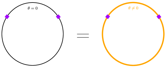
Figure 4: The figure illustrates one of the main conditions imposed in our derivation, where the thick orange line represents the line with the deformation switched on ($\theta\neq 0$), and the thin dark line represents the original 1D CFT with $\theta=0$. The inserted operators are $\frac{1}{2}$-BPS tilt operators with polarisation orthogonal to the plane of the $\theta$-rotation. We demand that such 2-point function should be invariant.

Rather than fixing completely the higher-order coefficients, we will impose some physical conditions that will result into sum rules. The conditions we will exploit descend from the fact that $\theta$ parametrises a symmetry of the CFT (when the parameter is switched on uniformly on the whole line). In particular, provided we properly redefine the operators, all correlation functions should not depend on $\theta$.

For our purposes, it will be enough to use two particularly simple cases. For example, the expectation value of the circular Wilson loop does not depend on $\theta$. This means that the vacuum expectation value of the deformed action should be invariant, in other words

$$\langle{\rm P}e^{\int_{0}^{2\pi}\delta L(t)}\rangle_{{1{\rm D}}}=1\,.$$ (63)

This condition is the simplest way to fix the coupling of the identity operator at order $\mathcal{O}(\mathbf{s}^{2})$, as we show in the next section.

Secondly, we will impose the invariance of certain 2-point functions, as illustrated in Figure 4. We consider 2-point functions involving two identical operators $\Phi_{\perp}^{M}$, where $M\in\left\{2,3,4,5\right\}$ is a direction orthogonal to $\theta$-deformation. We impose that this 2-point function should not depend on the deformation parameter,

$$\langle{\rm P}e^{\int_{0}^{2\pi}\delta L(t)}O_{\Phi_{\perp}^{M}}(t_{1})\,O_{\Phi_{\perp}^{M}}(t_{2})\rangle_{{1{\rm D}}}=\langle O_{\Phi_{\perp}^{M}}(t_{1})\,O_{\Phi_{\perp}^{M}}(t_{2})\rangle_{{1{\rm D}}}={\rm Pr}(t_{1},t_{2})\,.$$ (64)

Studying the latter condition we will deduce a sum rule which constrains all the coefficients $b_{n,2}$, for the operators $O_{n}$ in our OPE.

We will combine this information with the relation with the cusp anomalous dimension given by the defect configuration of Figure 3, and we will see that this leads us to the constraint we are after which is the main result of this paper. For convenience, we list here the key relation we are going to use, transforming the variables of (46) to the thermal circle:

$$\langle{\rm P}e^{\int_{t_{1}}^{t_{2}}\delta L(t)dt}\rangle_{{1{\rm D}}}\propto[\epsilon^{2}\;P(t_{1},t_{2})]^{\Gamma_{\rm cusp}(\theta)}\;,$$ (65)

where $\epsilon$ is the UV cutoff around the points $t_{i}$, and there is an unfixed, regularisation-dependent proportionality constant. We will see in the next section how we can easily remove such ambiguities and focus on the physical content of the equation.

As a final comment, let us notice that, in principle, the operators should also be redefined (rotated in R-space) with $\theta$ to ensure invariance of correlation functions. In general, operators would need to be redefined with an expression of the form,

$$O_{m}(t)\rightarrow O_{m}(t,\theta)=O_{m}(t)+\sum_{k=1}^{\infty}\mathbf{s}^{k}\;\sum_{n}M_{m,n}^{(k)}\;\epsilon^{\Delta_{n}-\Delta_{n}}O_{n}(t),$$ (66)

which certain coefficients $M_{m,n}$. The expectation drawn from the ${\cal N}=4$ SYM picture is that for operators taken orthogonal to the deformation, such redefinition is not necessary.

In the next section we will obtain the constraint originating from this invariance and then impose (58) to obtain the main result for the integrated correlator in closed form, independent on the Wilson coefficients.

3.4 Extra comments on the operators in the deformed action

Let us make some additional comments on the operators present in the deformed action. The $\mathcal{N}$=4 SYM formalism suggests that the only operators present beyond the leading order are $O_{\Phi_{||}}$ and $\mathds{1}$. However, in our conformal perturbation theory setup the symmetries of the original theory are somewhat obscured, and we cannot definitively exclude that something more general might happen in our regularisation scheme. Here, we briefly discuss what these operators might possibly be and how one could try to fix them. We emphasise, however, that these considerations are not needed for the derivation presented in the next section.

First, there are certainly some restrictions on the extra operators based on global symmetry considerations. In particular, the $\theta$-rotation on the whole line is a special case of a general symmetry on the conformal manifold, which preserves supersymmetry. We could consider a rotation by angle $\theta$ in a generic plane among the orthogonal directions in R-space, and this should be a natural covariant generalisation of our deformed action. At the leading order, such generic $\theta$-deformation would couple to a tilt operator $\delta L=\delta\vec{n}^{i}O_{\Phi_{\perp}^{i}}$, with $\delta n^{i}$ specifying a direction in R-space, with $\delta n^{i}\cdot(0,0,0,0,0,1)=0$ and $||\delta\vec{n}||=\mathbf{s}$. At next-to-leading order, the deformed action would need to couple to the two possible tensor structures built with $\delta\vec{n}^{i}\delta\vec{n}^{j}$, indicating that the operators in the action can only be either neutral under R-symmetry, or in the symmetric traceless representation $[2,0]$.

Another natural expectation is that, in any scheme, the only operators which can appear at higher orders in the deformation are the ones which can be built through the subsequent OPE’s of operators at lower orders. For example, at next-to-leading order $\mathcal{O}({\bf s}^{2})$ we would expect only operators in the OPE $\Phi_{\perp}^{1}\Phi_{\perp}^{1}\rightarrow O_{n}$ (3).

Further, the $\theta$-deformation on the whole line obviously preserves conformal symmetry. Therefore, the beta function for the coupling of every operator in the action should vanish, and remain vanishing as we move $\theta$. This should severely constrain the form of the Wilson coefficients. We did not tackle a computation of the beta functions in our scheme. However, we can make some contact with a well-known result of Cardy for the beta functions in conformal perturbation theory with a point-splitting cutoff Cardy:1996xt , which is usually applied to the case of marginal and relevant operators. For perturbations $S_{CFT}+\sum_{i}b_{i}\int ds\,{O}_{i}(s)$, the result of Cardy, specialised to $D=1$, reads

$$\beta_{i}=\epsilon\partial_{\epsilon}b_{i}=(1-\Delta_{i})b_{i}+\sum_{k,l}b_{k}b_{l}C_{kl}^{i}+\mathcal{O}(|b|^{3}),$$ (67)

where $C$’s are the OPE coefficients.

We can see how this result applies to our situation, where the Wilson coefficients $b_{i}$ additionally scale with $\theta$, $b_{i}=\sum_{k}b_{i,k}\mathbf{s}^{k}$. Consider the case of the marginal operator $O_{\Phi_{\perp}^{1}}$. Since by assumption $b_{\Phi_{\perp}^{1}}\equiv\mathbf{s}$ and there is no OPE coefficient $C_{\Phi_{\perp}^{1}\Phi_{\perp}^{1}\Phi_{\perp}^{1}}=0$, (67) simply confirms that $\beta_{\Phi_{\perp}^{1}}$ vanishes up to order $\mathcal{O}(\mathbf{s}^{2})$.

In the case of the identity operator $\mathds{1}$, relation (67) expanded up to the same order yields

$$\beta_{\mathds{1}}=b_{\mathds{1},2}\mathbf{s}^{2}+(2\mathbb{B})C_{\Phi_{\perp}^{1}\Phi_{\perp}^{1}\mathds{1}}\mathbf{s}^{2}+\mathcal{O}(\mathbf{s}^{3}),$$ (68)

with $C_{\Phi_{\perp}^{1}\Phi_{\perp}^{1}\mathds{1}}=1$, therefore from the vanishing of the beta function we get

$$b_{\mathds{1},2}=-2\mathbb{B}.$$ (69)

This is indeed what we will find, by an independent calculation, in the next section, see 72.

One would be tempted to apply (67) also to fix the couplings for the irrelevant operators. However, this does not seem to be consistent with our results, in particular with the sum rules deduced in the next section. We were also not able to reproduce the arguments of (67) in application to our specific regularisation scheme. A careful analysis would be needed in order to compute the beta functions for the irrelevant operators in our action, and we will not study this problem here.

In our derivation, we are fixing part of the couplings (or more precisely, sum rules for them) by computing some observables and imposing that they satisfy the physical invariances of the $\theta$-deformation. We have imposed such conditions only for a couple of special observables. We can imagine that imposing more constraints, in addition to the vanishing of the beta functions, would help fix the Wilson coefficients and clarify whether more operators on top of $\mathds{1}$ and $O_{\Phi_{||}}$ should be included in the action. Fixing precisely the couplings might be useful in some applications. In particular, we could use them to compute some physical observables – for example, one could consider “multi-cusp” correlators where different $\theta$’s are switched on on different segments of the line. Clarifying these points could be a fruitful potential direction for future studies, which, however is not critical for the derivation of this paper as we discuss in the next section.

4 Derivation of the integrated correlator involving the curvature function

We will use the formal approach described in the previous section to relate the curvature function with an integrated 4-point correlator. The derivation will be done in two steps: First we deduce a constraint on the Wilson coefficients $b_{n,k}$ from the requirement that the deformation by $\theta$ applied to the whole space should be a symmetry. More precisely we impose the properties (63) and (64). Second, we use the relation between the cusp anomalous dimension and the deformation applied to a part of the space (58) expanded to the forth order in ${\bf s}$. By using these two equations, we will be able to derive our final result: the linear combination of the two integrated correlators (39) and (40), complementary to the one derived in Drukker:2022pxk completing the derivation of the two relations found in Cavaglia:2022qpg .

4.1 Constraining the $b_{\mathds{1},2}$ coupling

We begin by considering the constraint (63) at the ${\rm O}({\bf s}^{2})$ order, which gives

$${\bf s}^{2}\,\left[\int_{\epsilon}^{2\pi}ds_{2}\int_{{\rm max}(0,s_{2}-2\pi+\epsilon)}^{s_{2}-\epsilon}ds_{1}\langle O_{\Phi_{\perp}^{1}}(s_{1})O_{\Phi_{\perp}^{1}}(s_{2})\rangle_{{1{\rm D}}}+\frac{b_{\mathds{1},2}}{\epsilon}\int_{0}^{2\pi}ds\right]=0\;,$$ (70)

where we explicitly written the regularisation of the integrals with the measure $\mu_{2}$ (59) that introduces the cutoff $\epsilon$ to prevent the coordinates $s_{1}$ and $s_{2}$ coming closer than $\epsilon$ to each other. The first term in (70) is the integrated two-point function of the marginal operator $O_{\Phi_{\perp}^{1}}$ while the second one is the contribution of the identity. Using the definition (8) and the normalisation (38), one can solve the integration, which gives

$$\int_{\epsilon}^{2\pi}ds_{2}\int_{{\rm max}(0,s_{2}-2\pi+\epsilon)}^{s_{2}-\epsilon}ds_{1}\frac{2{\mathbb{B}}}{2-2\cos(s_{1}-s_{2})}=\frac{4\pi{\mathbb{B}}}{\epsilon}+{\cal O}(\epsilon)\;,$$ (71)

thus we obtain

$$b_{\mathds{1},2}=-2\;\mathbb{B}\;,$$ (72)

which is in agreement with the argument in (69). We will use this relation in the next section.

4.2 Constraining a combination of $b_{n,2}$ couplings

Now we impose the constraint (64). We take equal indices $N=M$ from the beginning with $M\in\left\{2,3,4,5\right\}$ and expand to the order $\mathcal{O}({\bf s}^{2})$ to obtain for the coefficients of ${\bf s}^{2}$

$$0 = \underbrace{\frac{b_{0,2}}{\epsilon}\;\left(\int_{0}^{2\pi}ds\,\mu_{1,2}(s;t_{1},t_{2})\right)\,\langle O_{\Phi_{\perp}^{M}}(t_{1})O_{\Phi_{\perp}^{M}}(t_{2})\rangle_{{1{\rm D}}}}_{\text{identity contribution }\equiv\;\mathcal{I}_{1-\text{pt}}}$$

$$+\underbrace{\sum_{\Delta_{n}>1}\epsilon^{\Delta_{n}-1}b_{n,2}\int_{0}^{2\pi}ds\,\mu_{1,2}(s;t_{1},t_{2})\;\langle O_{\Phi_{\perp}^{M}}(t_{1}){O}_{n}(s)O_{\Phi_{\perp}^{M}}(t_{2})\rangle_{{1{\rm D}}}}_{\text{integrated 3-point }\equiv\;\mathcal{I}_{3-\text{pt}}}$$

$$+\underbrace{\int_{0<s_{1}<s_{2}<2\pi}ds_{1}ds_{2}\;\mu_{2,2}(s_{1},s_{2};t_{1},t_{2})\;\langle O_{\Phi_{\perp}^{M}}(t_{1})O_{\Phi_{\perp}^{1}}(s_{1})O_{\Phi_{\perp}^{1}}(s_{2})O_{\Phi_{\perp}^{M}}(t_{2})\rangle_{{1{\rm D}}}}_{\text{integrated 4-point }\equiv\;\mathcal{I}_{4-\text{pt}}},$$

where the integration measure $\mu_{n,m}$ enforce the hard-sphere cutoffs as defined in section 3.2. The contribution of the first line of (4.2) is given by the trivial integral of the measure $\mu_{1}$ and it reads

$$\mathcal{I}_{1-\text{pt}}=\frac{(2\pi-4{\epsilon})}{\epsilon}\,b_{\mathds{1},2}\,(2\mathbb{B}){\rm P}(t_{1},t_{2}),$$ (74)

with $b_{\mathds{1},2}=-2\mathbb{B}$ given by (72) and another $2\mathbb{B}$ coming from the special normalisation of the tilt operator $O_{\Phi_{\perp}^{M}}$. The remaining two terms are more involved and they are computed explicitly in appendix C.1. Integrated 3-point functions appearing in the second line can be obtained assuming a generic spectrum with $\Delta_{n}>1$ at finite coupling. Taking into account the kinematics (7) and normalisation (18), we find that the integral is finite and gives

$$\mathcal{I}_{3-\text{pt}}=(2\mathbb{B})\,{\rm P}(t_{1},t_{2})\;\sum_{\Delta_{n}>1}b_{n,2}\frac{4\,C_{n}}{\Delta_{n}-1}\;.$$ (75)

The final contribution is given by the 4-point functions in the last line of (4.2). In order to solve this integral it is convenient to use the parametrisation for $G(x)$ given in (11). Details of this calculation are described in appendix C and lead to the following result

$$\small\begin{split}\mathcal{I}_{4-\text{pt}}\!=\!(2\mathbb{B})^{2}\Biggl{(}\frac{2\pi\!-\!6{\epsilon}}{\epsilon}\!+\!\int_{0}^{\frac{1}{2}}\!\!dx\!\left[\frac{\delta G_{3}(x)}{x^{2}}\log{x}+\frac{\delta G_{1}(x)}{x^{2}}\log{\frac{x^{2}}{1\!-\!x}}+\frac{\delta G_{2}(x)}{x^{2}}\log{\frac{x}{1\!-\!x}}\right]\!\!\Biggl{)}{\rm P}(t_{1},t_{2}),\end{split}$$ (76)

where $\delta G_{i}(x)=G_{i}(x)-G_{i,\text{tree}}(x)$ with $G_{i}(x)$ are given in (12) and their tree-level values are

$$G_{1,\text{tree}}(x)=1\;,\qquad G_{2,\text{tree}}(x)=0\;,\qquad G_{3,\text{tree}}(x)=\frac{x^{2}}{(x-1)^{2}}\;.$$ (77)

Notice that the integration in (76) goes in the domain $[0,1/2]$ and, unfortunately, there is no way to extend it to the whole interval $[0,1]$ using crossing (20) in a smooth way. This is a manifestation of the scheme dependence of the Wilson coefficients. However, we will see, that in the final result, which only contains physical quantities, the integration can be extended to the whole range naturally.

Once all pieces are combined, from $\mathcal{I}_{1-\text{pt}}+\mathcal{I}_{3-\text{pt}}+\mathcal{I}_{4-\text{pt}}=0$ we find

$$\!\!\!\!\!\!\sum_{\Delta_{n}>1}\!b_{n,2}\frac{C_{n}}{\Delta_{n}\!-\!1}+\mathbb{B}\!\!\int_{0}^{\frac{1}{2}}\!\!dx\!\left[\frac{\delta G_{3}(x)}{x^{2}}\log{x}+\frac{\delta G_{1}(x)}{x^{2}}\log{\frac{x^{2}}{1\!-\!x}}+\frac{\delta G_{2}(x)}{x^{2}}\log{\frac{x}{1\!-\!x}}\right]\!=\!\mathbb{B}.$$ (78)

This can be seen as a constraint on the weighted sum of the couplings $b_{n,2}$ in terms of the CFT data. At the same time, if we assume that only $O_{\Phi_{||}}$ contributes, the above relation completely fixes the value of the only coefficient $b_{\Phi_{||},2}$! We will use this assumption to analyse $b_{1,2}$ in section 4.4.

Finally, let us rewrite the main result of this section (78) in terms of the reduced amplitude $\delta f(x)=f(x)-f_{\rm free}(x)$, as defined in (12) and (41)

$$\frac{1}{\mathbb{B}}\!\sum_{\Delta_{n}>1}\!b_{n,2}\frac{C_{n}}{\Delta_{n}-1}=\!\int_{\delta_{x}}^{\frac{1}{2}}\!dx\frac{(x\!-\!2)\delta f(x)}{x^{3}}-(3-\mathbb{F})\log(\delta_{x})+(\mathbb{F}-2)\,\log(2)+1.$$ (79)

Note that the r.h.s. of (79) is finite in the limit in which the cutoff $\delta_{x}\rightarrow 0^{+}$ since $\delta f(x)\sim\frac{3-\mathbb{F}}{2}x^{2}$ for $x\rightarrow 0$.

In order to get a closed expression for the integrated correlator, in the next section we make another calculation involving deformation only on a part of the thermal circle of the 1D CFT.

4.3 Matching with the cusp anomalous dimension

So far we obtained the nontrivial equation (79) involving the Wilson coefficients $b_{n,2}$ relating them to the OPE coefficients $C_{n}$ and ${\mathbb{B}}$ and to an integral of the reduced correlator $f(x)$. In this section we exploit the cusp deformation introduced in section 2.3 to conclude our derivation. We start from the equation  (65), which can be written in the form

$$\langle{\rm P}e^{\int_{t_{1}}^{t_{2}}\delta L(t)dt}\rangle_{{1{\rm D}}}=K\;[P(t_{1},t_{2})]^{\Gamma_{\rm cusp}(\theta)}\;,$$ (80)

where $K$ is a non-physical renormalisation constant (e.g. depending on the UV cutoffs), while $\Gamma_{\text{cusp}}(\theta)$, independent on the scheme, is the cusp anomalous dimension discussed in section 2.3. In order to get rid of the constant $K$ we consider the following expression

$$\l\frac{\partial_{t_{1}}\partial_{t_{2}}\log{\langle{\rm P}e^{\int_{t_{1}}^{t_{2}}\delta L(t)dt}\rangle_{{1{\rm D}}}}}{{\rm P}(t_{1},t_{2})}=-2\Gamma_{\text{cusp}}(\theta)\;,$$ (81)

as follows from (80). Notice that now both l.h.s. and r.h.s. are finite quantities. Next we expand both sides in powers of ${\bf s}$. It is useful to denote the expansion coefficients as follows

$$\langle{\rm P}e^{\int_{t_{1}}^{t_{2}}\delta L(t)dt}\rangle_{{1{\rm D}}}=1+A(t_{1},t_{2})\,{\bf s}^{2}+B(t_{1},t_{2})\,{\bf s}^{4}+\mathcal{O}({\bf s}^{6}),$$ (82)

where $A(t_{1},t_{2})$ and $B(t_{1},t_{2})$ are defined explicitly in appendix B and contain contributions from various integrated correlation functions, schematically

$$A(t_{1},t_{2})=(\texttt{1-pt})+(\texttt{2-pt}),\;\;\;B(t_{1},t_{2})=(\texttt{1-pt})+(\texttt{2-pt})+(\texttt{3-pt})+(\texttt{4-pt})\,.$$ (83)

Those terms can also be seen from (3.1.1). The only difference is that we allow now for multiple $O_{n}$ and not only $\Phi_{||}$.

Even though we only have the action (54) at the order ${\bf s}^{2}$, it is easy to convince ourselves that only the identity operator at order ${\bf s}^{4}$ can contribute (which we do take into account), but nothing else which could appear in the action at higher orders. The function $A(t_{1},t_{2})$ takes contributions from the integrated 1-point functions (of the identity operator), as well as 2-point function of the line-deformation operator $O_{\Phi_{\perp}^{1}}$, while $B(t_{1},t_{2})$ contains contributions from: integrated 1-point function of the identity operator at the next order, integrated 2-point functions of generic operators in the action, integrated 3-point functions involving two $O_{\Phi_{\perp}^{1}}$ and a third generic operator and integrated 4-point correlators of the line-deformation scalars. From the above expansion it follows

$$\log\,\langle{\rm P}e^{\int_{t_{1}}^{t_{2}}\delta L(t)dt}\rangle_{{1{\rm D}}}=A(t_{1},t_{2})\,{\bf s}^{2}+\bigg{[}B(t_{1},t_{2})-\frac{A^{2}(t_{1},t_{2})}{2}\bigg{]}\,{\bf s}^{4}+\mathcal{O}({\bf s}^{6})\;.$$ (84)

In the following we compute the two combinations appearing in (84) in terms of the Bremsstrahlung (29) and Curvature functions (30) arising from the expansion of the cusp anomalous dimension.

First order.

At leading order in ${\bf s}$, (81) becomes

$$\frac{\partial_{t_{1}}\partial_{t_{2}}A(t_{1},t_{2})}{{\rm P}(t_{1},t_{2})}=-2\mathbb{B}\,.$$ (85)

As from (B) we have

$$\partial_{t_{1}}\partial_{t_{2}}A(t_{1},t_{2})=-\langle O_{\Phi_{\perp}^{1}}(t_{1})O_{\Phi_{\perp}^{1}}(t_{2})\rangle_{{1{\rm D}}}\,,$$ (86)

the equation (85) does indeed hold as a consequence of the 2-point function normalisation (38).

Next-to-leading order.

The next-to-leading order constraint deriving from (81) reads

$$\frac{\partial_{t_{1}}\partial_{t_{2}}\left(B(t_{1},t_{2})-\frac{A^{2}(t_{1},t_{2})}{2}\ \right)}{{\rm P}(t_{1},t_{2})}=-\frac{\mathbb{B}+\mathbb{C}}{2}.$$ (87)

The evaluation of the l.h.s. in our regularisation scheme is rather long, and is spelled out in appendices (the final result is deduced in (B), relying on explicit calculations which are stored in appendix C). The main nontrivial contributions, as in the calculation of the previous section, come from the integrated 3-point functions of the type $\langle O_{\Phi_{\perp}^{1}}O_{\Phi_{\perp}^{1}}O_{n}\rangle_{{1{\rm D}}}$ as well as from the integrated 4-point function $\langle O_{\Phi_{\perp}^{1}}O_{\Phi_{\perp}^{1}}O_{\Phi_{\perp}^{1}}O_{\Phi_{\perp}^{1}}\rangle_{{1{\rm D}}}$. After the dust settles, the divergences cancel and (87) becomes

$$\begin{split}-\frac{1}{2}\left(\mathbb{C}+\mathbb{B}\right)&=-(2\mathbb{B})\sum_{\Delta_{n}>1}\;b_{n,2}\;\frac{4C_{n}}{\Delta_{n}-1}-(2\mathbb{B})^{2}(2-\mathbb{F})\,\left(1+\log 4\right)+4\;\mathbb{B}^{2}\\ &-(2\mathbb{B})^{2}\,\left[\int_{\delta_{x}}^{\frac{1}{2}}dx\frac{(2x-3)((x-1)x+1)\delta f(x)}{(x-1)x^{3}}\,dx+\frac{3}{2}(3-\mathbb{F})\log\delta_{x}\right].\end{split}$$ (88)

Notice that the sum, containing the Wilson coefficients, appearing in (88) is exactly the same as in (79). Thus we can exclude them completely obtaining a closed expression for the integrated correlator.

A new linear combination of integrated correlators.

Substituting in (88) the sum over the Wilson coefficients $b_{n,2}$ given by (79), we obtain

$$-\frac{\mathbb{C}+\mathbb{B}}{8\,\mathbb{B}^{2}} = -3+\mathbb{F}+\frac{1}{2}(3-\mathbb{F})\log{\delta_{x}}+\int_{\delta_{x}}^{\frac{1}{2}}dx\;\delta f(x)\left(\frac{1}{x^{3}}-\frac{3}{x}+\frac{1}{x-1}\right),$$ (89)

which is a constraint involving only CFT data. This is the main result of our derivation. It is simple to verify that (89) is a linear combination of the two constraints (39) and (40) originally found in Cavaglia:2022qpg . Indeed, using crossing symmetry (20) to rearrange the integration domain, they can be rewritten as follows

Constraint1: $$\int_{\delta_{x}}^{\frac{1}{2}}\!\delta f(x)\!\left(\frac{1}{x^{3}}\!-\!\frac{2}{x^{2}}\!+\!\frac{1}{x}\!+\!\frac{1}{x\!-\!1}\!\right)\!dx+\frac{3\!-\!\mathbb{F}}{2}\log{\delta_{x}}\!+\!3\!-\!\mathbb{F}=\frac{3\mathbb{C}\!-\!\mathbb{B}}{8\mathbb{B}^{2}},$$ (90)

Constraint2: $$\int_{0}^{\frac{1}{2}}\!\delta f(x)\left(\frac{1}{x}-\frac{1-x}{x^{2}}\right)dx=\frac{\mathbb{C}}{4\mathbb{B}^{2}}+\mathbb{F}-3.$$ (91)

Combining (90) and (91) with coefficients $1\times\texttt{Constraint1}-2\times\texttt{Constraint2}$, it is simple to verify that (89) is perfectly reproduced. This, together with the combination $-2\times\texttt{Constraint1}+3\times\texttt{Constraint2}$ (45) derived in Drukker:2022pxk we conclude the proof of those relations.

4.4 Normalisation of $\Phi_{||}$

Assuming that only the operator $O_{\Phi_{||}}$ contributes to the sum in (53), it is possible to link our conformal perturbation theory setup with the usual ${\cal N}=4$ SYM expression for the MWL computing the only remaining Wilson coefficient $b_{1,2}\equiv b_{\Phi_{||},2}$. In order to evaluate it, we can exploit the constraint (79). Using it we can evaluate $b_{1,2}$ analytically both at weak and strong coupling, from the known expression for $f(x)$ Kiryu:2018phb ; Cavaglia:2022qpg ; Ferrero:2021bsb .

Weak coupling.

At weak coupling, the integral of $f(x)$ has to be treated carefully. Indeed, it contains an anomalous term given by the divergence of the superconformal block of the long-multiplet at $x\sim 0$ for $\Delta_{1}=1$. Following the same logic of Cavaglia:2022qpg , we can quantify the “anomaly” term to be $2C_{1}^{2}/(\Delta_{1}-1)^{2}$ (in the terminology of Cavaglia:2022qpg ). Details of the computation are given in appendix D. Using the regularisation given in (171), the integral appearing in (79) is computed using the representation of $f(x)$ in terms of harmonic polylogarithms (HPL) implemented in the Mathematica package Maitre:2005uu . Using the HPL’s properties, the integral can be solved recursively using integration by parts. Plugging it in the constraint (79) and solving for $b_{1,2}$ we have

$$b_{1,2} =\frac{g}{\sqrt{2}}-\frac{g^{3}\left(\pi^{2}-6\right)}{3\sqrt{2}}+\frac{g^{5}\left(-108(\zeta_{3}+3)+12\pi^{2}+5\pi^{4}+576\log 2\right)}{18\sqrt{2}}+...\,,$$ (92)

where $...$ stand for higher orders in the coupling. An additional order is presented in appendix D. Notice that, the sign of the result (92) depends on the choice of the one of the square root of $C_{1}^{2}$, while the sign of the product $b_{1,2}\,C_{1}$ is fixed. We chose the positive sign for the square root.

Strong coupling.

In this regime the integral in (79) does not have any additional divergences. Strong coupling data are given in Ferrero:2021bsb . Similarly to the weak coupling case, the integral is computed using the representation of $f(x)$ in terms of Harmonic polylogarithms. The integral is divergent for $\delta_{x}\rightarrow 0$, but all the divergences are nicely cancelled by the $(3-\mathbb{F})\log\delta_{x}$ regulator as expected. We obtain

$$b_{1,2}\!=\!\frac{\!1\!\!+\!\log 2}{\sqrt{2/5}\,\pi}g\!-\!\frac{\!\!149\!-\!8\pi^{2}\!+\!17\log 2}{96\,\sqrt{2/5}\,\pi^{2}}\!+\!\frac{\!\!5616\zeta_{3}\!+\!21003\!-\!1232\pi^{2}\!+\!45\log 2(256\log 2\!-\!129)}{18432\,\sqrt{2/5}\,\pi^{3}g}\!+\!...$$ (93)

where $...$ stand for higher orders in $1/g$. Two additional orders are included in appendix D.

Comparison with field normalisation.

Now comparing (48) and (54) at the order ${\bf s}^{2}$ we conclude that we should impose, in the case when only one marginal operator contributes

$$\Phi_{||}=-2b_{1,2}\epsilon^{\Delta_{1}-1}O_{\Phi_{||}}\,.$$ (94)

The operator $O_{\Phi_{||}}$ has the standard unit normalisation in our conventions, from where we can conclude that the scalar of ${\cal N}=4$ SYM has to be normalised as follows

$$\langle\langle\Phi_{||}(t_{1})\;\Phi_{||}(t_{2})\rangle\rangle=4b_{1,2}^{2}\epsilon^{2\Delta_{1}-2}\frac{\delta_{ij}}{x_{12}^{2\Delta_{i}}}\;.$$ (95)

As from above we know $b_{1,2}$, this would then give us the normalisation of the non-protected scalar $\Phi_{||}$ in our regularisation scheme. We can now quickly test this relation at weak coupling: at the leading order there should not be difference between normalisation of $\Phi_{||}$ and $\Phi_{\perp}$ as at tree level there is no interaction with the MWL, thus $4b_{1,2}^{2}\epsilon^{2\Delta_{1}-2}$ should coincide with $2{\mathbb{B}}\simeq 2g^{2}$ at the leading order, which is indeed the case as one case see from (92). Furthermore, we notice that $\sqrt{{\mathbb{B}}/2}\simeq\frac{g}{\sqrt{2}}-\frac{\pi^{2}g^{3}}{3\sqrt{2}}+\frac{5\pi^{4}g^{5}}{18\sqrt{2}}+O\left(g^{6}\right)$ reproduces all terms in $b_{1,2}^{2}$ with maximal power of $\pi$, but otherwise there is no reason for the scalars to have the same normalisation beyond the leading order, as one is protected and the other is not in the interacting case.

5 Discussion

In this paper, we completed the proof of the integral constraints presented in Cavaglia:2022qpg . A linear combination of those relations was already derived in Drukker:2022pxk using a geometrical approach. Here, exploiting the invariance of the defect CFT under R-space rotation and relating it to the generalised cusp anomalous dimension, we provided the derivation of second relation, thereby completing the proof.

A possible future direction is to derive constraints on multi-point correlation functions e.g. 6-point functions, which should be related to the higher orders in expansion of the generalised cusp anomalous dimension with respect to the $\theta$ and $\phi$ deformations. Finding a shortcut method for deriving such relations between the correlation functions and the spectrum of the deformations would generate, in principle, an infinite amount of additional constraints on the 1D CFT, which could be sufficient for its complete solution. We also expect that at each order there should be an increasing number of such constraints – like we found $2$ of them for $4$-point function, one could speculate that there should be at least $3$ non-trivial constraints for $6$-point functions. We also note that the data coming from the integrability side become richer with each order in $\theta$ or $\phi$: the Bremsstrahlung function contains only powers of $\pi$ in its perturbation theory, the Curvature function already brings in zeta functions, and we expect MZV’s to come from the next order as well. The higher point correlation functions in the current context were studied recently in Barrat:2021tpn ; Barrat:2022eim at weak coupling, which could give a starting point in this investigation.

Furthermore, one can use the integrability data for the cusp with arbitrary operators sitting at the cusp, to constrain more complicated correlators with non-BPS external legs.

Another interesting direction is to extend our derivation to other integrable gauge theories. The most natural choice would be the three-dimensional ABJM theory where 1D superconformal defect theories supported by Wilson loops were defined in Bianchi:2017ozk ; Bianchi:2018scb and recently studied in Bianchi:2020hsz ; Gorini:2022jws . The cusp anomalous dimension was studied in Griguolo:2012iq ; Bonini:2016fnc and the Bremsstrahlung function is known exactly Bianchi:2014laa ; Correa:2014aga ; Bianchi:2017svd ; Bianchi:2018scb (see also Drukker:2019bev ). The curvature function is still not known since an integrability formulation for the cusped Wilson line is still lacking. However, all the conformal perturbation theory approach we have described seems ready for application in this context, and also the geometrical argument of Drukker:2022pxk should lead to a new non-trivial constraint for the line defect in ABJM theory.

It would be also interesting to investigate the fishnet limit Erickson:1999qv ; Zamolodchikov:1980mb ; Gurdogan:2015csr ; Caetano:2016ydc ; Kazakov:2018gcy ; Pittelli:2019ceq ; Gromov:2021ahm and integrated operators in this simpler theory, where one can hope to advance analytically more easily and in particular to get the answer to the fundamental question if integrability for the spectrum in combination with conformal symmetry is sufficient to solve this type of beyond-the-spectrum observables.

Appendix A The curvature function

The Curvature function was computed by means of QSC in terms of a double contour integral in  Gromov:2015dfa . In the $\phi\rightarrow 0$ limit, it reduces to (30) where the kernel is is given by

$$K_{0}(u)=\partial_{u}\log\frac{\Gamma(iu+1)}{\Gamma(-iu+1)}\,,$$ (96)

and the integrand $F$ is

$$F[x,y] =-\frac{8i\sinh\left(2\pi u_{x}\right)u_{x}u_{y}x^{2}S_{0}(y)}{I_{1}(4g\pi){}^{2}}$$

$$+S_{0}(y){}^{2}\left[\frac{8ixyI_{2}(4g\pi)u_{x}u_{y}}{g\pi\left(x^{2}-1\right)I_{1}(4g\pi){}^{3}}-\frac{8ixyI_{2}(4g\pi)u_{x}u_{y}}{g\pi\left(y^{2}-1\right)I_{1}(4g\pi){}^{3}}+\frac{32ixyu_{x}u_{y}}{I_{1}(4g\pi){}^{2}}\right]$$

$$+\sinh^{2}\left(2\pi u_{y}\right)\left[\frac{4ixyI_{2}(4g\pi)u_{x}u_{y}}{g\pi\left(x^{2}-1\right)I_{1}(4g\pi){}^{3}}+\frac{16ixyu_{x}u_{y}}{I_{1}(4g\pi){}^{2}}\right]$$

$$+\sinh\left(2\pi u_{y}\right)\left[\frac{4ixu_{x}u_{y}y^{2}}{\left(x^{2}-1\right)I_{1}(4g\pi)}-\frac{8ix\sinh\left(2\pi u\right)u_{x}u_{y}y}{I_{1}(4g\pi){}^{2}}-\frac{8iu_{x}u_{y}S_{1}(x)y}{gI_{1}(4g\pi){}^{2}}\right.$$

$$\left.-\frac{16ixu_{x}u_{y}}{\left(y^{2}-1\right)I_{1}(4g\pi)}+\left(-\frac{8ixyI_{2}(4g\pi)u_{x}u_{y}}{g\pi\left(x^{2}-1\right)I_{1}(4g\pi){}^{3}}-\frac{32ixyu_{x}u_{y}}{I_{1}(4g\pi){}^{2}}\right)S_{0}(y)\right]$$

$$+S_{1}(y)\left[\frac{8ixyu_{x}u_{y}}{g\left(x^{2}-1\right)I_{1}(4g\pi)}-\frac{8ixyu_{x}u_{y}}{g\left(y^{2}-1\right)I_{1}(4g\pi)}\right]$$

$$+S_{0}(x)\left[S_{0}(y)\left(\frac{16iu_{x}u_{y}}{I_{1}(4g\pi){}^{2}}-\frac{16iy^{2}u_{x}u_{y}}{I_{1}(4g\pi){}^{2}}\right)-\frac{4ixI_{2}(4g\pi)u_{x}u_{y}S_{1}(y)}{g^{2}\pi\left(x^{2}-1\right)I_{1}(4g\pi){}^{3}}\right]$$

$$+ S_{0}(y)\left[\frac{8ixu_{x}u_{y}y^{2}}{\left(x^{2}-1\right)I_{1}(4g\pi)}+\frac{8ixu_{x}u_{y}}{I_{1}(4g\pi)}-\frac{8ixu_{x}u_{y}}{\left(x^{2}-1\right)I_{1}(4g\pi)}+\frac{32ixu_{x}u_{y}}{\left(y^{2}-1\right)I_{1}(4g\pi)}\right.$$

$$\left.+S_{1}(x)\left(-\frac{4ixI_{2}(4g\pi)u_{x}u_{y}}{g^{2}\pi\left(x^{2}-1\right)I_{1}(4g\pi){}^{3}}-\frac{16ixu_{x}u_{y}}{gI_{1}(4g\pi){}^{2}}\right)\right.$$

$$\left.+S_{1}(y)\left(\frac{4ixI_{2}(4g\pi)u_{x}u_{y}}{g^{2}\pi\left(x^{2}-1\right)I_{1}(4g\pi){}^{3}}+\frac{16ixu_{x}u_{y}}{gI_{1}(4g\pi){}^{2}}\right)\right],$$

with

$$S_{0}(x)=\sum\limits_{n=1}^{\infty}\frac{I_{2n+1}(4\pi g)}{x^{2n+1}},\ \ \ S_{1}(x)=\sum\limits_{n=1}^{\infty}\frac{2nI_{2n}(4\pi g)}{\pi x^{2n}}\;.$$ (98)

These are functions of $x$, $y$ that are related to $u_{x}$, $u_{y}$ by the usual Zhukovsky map

$$x+\frac{1}{x}=\frac{u_{x}}{g},\ \ \ |x|\geq 1\ ,$$ (99)

(same for $y$, $u_{y}$), which resolves the cut $[-2g,2g]$ around which the integrals in (30) run. We attach with this paper, a Mathematica notebook “Curvature.nb” which computes the curvature function numerically for a given value of the coupling $g$.

Appendix B Expansion of the segment

The quantities $A$, $B$ appearing in (82) are defined through the following expansion

$$\begin{split}\bigg{\langle}\;\text{P\,exp}\biggl{[}\int_{t_{1}}^{t_{2}}dt\,\biggl{(}{\bf s}\;O_{\Phi_{\perp}^{1}}(t)+\sum_{\Delta_{n}>1}&\epsilon^{\Delta_{n}-1}\,O_{n}(t)\,\sum_{k=2}^{\infty}b_{n,k}\,{\bf s}^{k}\,\biggl{)}\biggl{]}\;\bigg{\rangle}_{1{\rm D}}\\ &\equiv 1+{\bf s}^{2}\;A(t_{1},t_{2})+{\bf s}^{4}\;B(t_{1},t_{2})+\dots.\end{split}$$ (100)

The leading order receives contributions from integrated 1- and 2-point functions such that

$$A(t_{1},t_{2})=K_{\mathds{1}}^{\text{1-pt}}+K^{\text{2-pt}},$$ (101)

with the explicit integrals given by

$$K_{\mathds{1}}^{\text{1-pt}} \equiv \frac{b_{0,2}}{\epsilon}\int_{t_{1}}^{t_{2}}ds\;\mu_{1,2}\;\langle\mathds{1}(s)\rangle_{1{\rm D}},$$ (102)

$$K^{\text{2-pt}} \equiv \int_{t_{1}<s_{1}<s_{2}<t_{2}}ds_{1}\,ds_{2}\;\mu_{2,2}\;\,\langle O_{\Phi_{\perp}^{1}}(s_{1})O_{\Phi_{\perp}^{1}}(s_{2})\rangle_{1{\rm D}}\;,$$ (103)

where the integration measures $\mu_{n,m}$ enforcing the cutoff is given in (61).

The next-to-leading order $B(t_{1},t_{2})$ is defined by the sum

$$B(t_{1},t_{2})=L_{\mathds{1}}^{\text{1-pt}}+L_{\mathds{1}}^{\text{2-pt}}+L_{\mathds{1}}^{\text{3-pt}}+\sum_{\Delta_{n}>1}\left(L_{O_{n}}^{\text{2-pt}}+L_{O_{n}}^{\text{3-pt}}\right)+L^{\text{4-pt}}.$$ (104)

The contributions involving the identity are given by

$$L_{\mathds{1}}^{\text{1-pt}} \equiv\frac{b_{0,4}}{\epsilon}\int_{t_{1}}^{t_{2}}ds\;\mu_{1,2}\;\langle\mathds{1}(s)\rangle_{1{\rm D}}\;,$$ (105)

$$L_{\mathds{1}}^{\text{2-pt}} \equiv\frac{b_{0,2}^{2}}{\epsilon^{2}}\;\int_{t_{1}<s_{1}<s_{2}<t_{2}}ds_{1}\,ds_{2}\;\mu_{2,2}\;\langle\mathds{1}(s_{1})\mathds{1}(s_{2})\rangle_{1{\rm D}}\;,$$ (106)

$$L_{\mathds{1}}^{\text{3-pt}} \equiv\frac{b_{0,2}}{\epsilon}\;\int_{t_{1}<s_{1}<s_{2}<s_{3}<t_{2}}ds_{1}\,ds_{2}\,ds_{3}\;\mu_{3,2}\;{\Big{[}}\langle\mathds{1}(s_{1})O_{\Phi^{1}_{\perp}}(s_{2})O_{\Phi^{1}_{\perp}}(s_{3})\rangle_{1{\rm D}}$$ (107)

$$\qquad\qquad\qquad\qquad\qquad+\langle O_{\Phi^{1}_{\perp}}(s_{1})\mathds{1}(s_{2})O_{\Phi^{1}_{\perp}}(s_{3})\rangle_{1{\rm D}}+\langle O_{\Phi^{1}_{\perp}}(s_{1})O_{\Phi^{1}_{\perp}}(s_{2})\mathds{1}(s_{3})\rangle_{1{\rm D}}{\Big{]}}\;.$$

The contributions involving $O_{n}$ are given by

$$L_{O_{n}}^{\text{2-pt}} \equiv{b^{2}_{n,2}}\,{\epsilon^{2\Delta_{n}-2}}\;\int_{t_{1}<s_{1}<s_{2}<t_{2}}ds_{1}\,ds_{2}\;\mu_{2,2}\;\langle O_{n}(s_{1})O_{n}(s_{2})\rangle_{1{\rm D}}\;,$$ (108)

$$L_{O_{n}}^{\text{3-pt}} \equiv{b_{n,2}}\,{\epsilon^{\Delta_{n}-1}}\;\int_{t_{1}<s_{1}<s_{2}<s_{3}<t_{2}}ds_{1}\,ds_{2}\,ds_{3}\;\mu_{3,2}\;{\Big{[}}\langle{O_{n}}(s_{1})O_{\Phi^{1}_{\perp}}(s_{2})O_{\Phi^{1}_{\perp}}(s_{3})\rangle_{1{\rm D}}$$ (109)

$$\qquad\qquad\qquad\qquad+\langle O_{\Phi^{1}_{\perp}}(s_{1}){O_{n}}(s_{2})O_{\Phi^{1}_{\perp}}(s_{3})\rangle_{1{\rm D}}+\langle O_{\Phi^{1}_{\perp}}(s_{1})O_{\Phi^{1}_{\perp}}(s_{2})O_{n}(s_{3})\rangle_{1{\rm D}}{\Big{]}}\;.$$

Finally, the $4-$point contribution of $O_{\Phi_{\perp}^{1}}$ is

$$L^{\text{4-pt}} \equiv\!\!\int_{t_{1}<s_{1}<s_{2}<s_{3}<s_{4}<t_{2}}\!\!\!\!\!\!\!\!\!\!\!\!ds_{1}\,ds_{2}\,ds_{3}\,ds_{4}\;\mu_{4,2}\;\langle O_{\Phi^{1}_{\perp}}(s_{1})O_{\Phi^{1}_{\perp}}(s_{2})O_{\Phi^{1}_{\perp}}(s_{3})O_{\Phi^{1}_{\perp}}(s_{4})\rangle_{1{\rm D}}\;.$$ (110)

Rather than evaluating this contribution directly, we note that what enters our derivation is the expression differentiated w.r.t. the endpoints $t_{1}$, $t_{2}$. These parameters enter the expression as integration limits, and differentiating removes two integrations. We then find

$$\partial_{t_{2}}\partial_{t_{1}}A(t_{1},t_{2}) =-\langle O_{\Phi_{\perp}^{1}}(t_{1}+\epsilon)O_{\Phi_{\perp}^{1}}(t_{2}-\epsilon)\rangle_{1{\rm D}}$$

$$=-2\mathbb{B}\,{\rm P}(t_{1}+{\epsilon},t_{2}-{\epsilon})=-2\mathbb{B}\,{\rm P}(t_{1},t_{2})+\mathcal{O}({\epsilon}).\;$$ (111)

Plugging this expression into the first order expansion (85), we see that we get a match. Next, we need the two combinations in (87). Let us start with the term involving $A(t_{1},t_{2})$. We get

$$\frac{1}{2}\partial_{t_{2}}\partial_{t_{1}}A^{2}(t_{1},t_{2})=\frac{1}{2}\partial_{t_{2}}\partial_{t_{1}}\bigg{[}K_{\mathds{1}}^{\texttt{1-pt}}\bigg{]}^{2}+\frac{1}{2}\partial_{t_{2}}\partial_{t_{1}}\bigg{[}K^{\texttt{2-pt}}\bigg{]}^{2}+\partial_{t_{2}}\partial_{t_{1}}\bigg{[}K_{\mathds{1}}^{\texttt{1-pt}}\times K^{\texttt{2-pt}}\bigg{]}\;,$$ (112)

where the differentiated kernels are given by

$$\partial_{t_{2}}\partial_{t_{1}}\bigg{[}K_{\mathds{1}}^{\texttt{1-pt}}\bigg{]}^{2} =-2\,\frac{b_{0,2}^{2}}{\epsilon^{2}}\;,$$ (113)

$$\partial_{t_{2}}\partial_{t_{1}}\bigg{[}K^{\texttt{2-pt}}\bigg{]}^{2} =\partial_{t_{2}}\partial_{t_{1}}\bigg{[}\int_{t_{1}+\epsilon}^{t_{2}-2\epsilon}ds_{1}\int_{s_{1}+\epsilon}^{t_{2}-\epsilon}ds_{2}\,\langle O_{\Phi^{1}_{\perp}}(s_{1})O_{\Phi^{1}_{\perp}}(s_{2})\rangle_{1{\rm D}}\bigg{]}^{2}\;,$$ (114)

$$\partial_{t_{2}}\partial_{t_{1}}\bigg{[}K_{\mathds{1}}^{\texttt{1-pt}}\times K^{\texttt{2-pt}}\bigg{]} =-\frac{b_{0,2}}{\epsilon}\int_{t_{1}+\epsilon}^{t_{2}-2\epsilon}ds_{1}\,\langle O_{\Phi_{\perp}^{1}}(s_{1})O_{\Phi_{\perp}^{1}}(t_{2}-\epsilon)\rangle_{1{\rm D}}$$ (115)

$$\!\!\!\!\!\!\!\!\!\!\!\!\!\!\!\!\!\!\!\!\!\!\!\!\!\!\!\!\!\!\!\!\!\!\!\!\!\!\!\!\!\!\!\!\!\!\!\!\!\!\!\!\!\!\!\!\!\!\!-\frac{b_{0,2}}{\epsilon}\int_{t_{1}+2\epsilon}^{t_{2}-\epsilon}ds_{2}\,\langle O_{\Phi_{\perp}^{1}}(t_{1}+\epsilon)O_{\Phi_{\perp}^{1}}(s_{2})\rangle_{1{\rm D}}-\frac{b_{0,2}}{\epsilon}(t_{2}-t_{1}-2\epsilon)\,\langle O_{\Phi_{\perp}^{1}}(t_{1}+\epsilon)O_{\Phi_{\perp}^{1}}(t_{2}-\epsilon)\rangle_{1{\rm D}}\;.$$

The integral (114) will be evaluated in combination with the four-point function (123). On the other hand, integral (115) can be computed easily by itself. Indeed, Taylor expanding in $\epsilon$ and discarding terms $\mathcal{O}(\epsilon)$, we get

$$\partial_{t_{2}}\partial_{t_{1}}\bigg{[}K_{\mathds{1}}^{\texttt{1-pt}}\times K^{\texttt{2-pt}}\bigg{]}=-\frac{4\,\mathbb{B}\,b_{0,2}}{\epsilon^{2}}+\frac{\mathbb{B}\,b_{0,2}}{3}\\ -\frac{2\,\mathbb{B}\,b_{0,2}}{\epsilon}\bigg{[}\Big{(}t_{2}-t_{1}-2\epsilon-2\,\sin(t_{2}-t_{1}-2\epsilon)\Big{)}{\rm P}(t_{1}+{\epsilon},t_{2}-{\epsilon})\bigg{]}+\mathcal{O}(\epsilon)\;.$$ (116)

Next, we evaluate the derivative with respect to $t_{1}$ and $t_{2}$ of $B(t_{1},t_{2})$. We display the result term by term. Let’s consider first the contributions involving the identity operator. Integrated one- and two-point functions are simply given by

$$\partial_{t_{1}}\partial_{t_{2}}L_{\mathds{1}}^{\text{1-pt}}=0\;,\qquad\partial_{t_{1}}\partial_{t_{2}}L_{\mathds{1}}^{\text{2-pt}}=-\frac{b_{0,2}^{2}}{\epsilon^{2}}\;,$$ (117)

while the three-point one is

$$\partial_{t_{1}}\partial_{t_{2}}L_{\mathds{1}}^{\text{3-pt}}=-\frac{b_{0,2}}{\epsilon}\int_{t_{1}+2\epsilon}^{t_{2}-2\epsilon}ds_{2}\bigg{[}\langle O_{\Phi_{\perp}^{1}}(t_{1}+\epsilon)O_{\Phi_{\perp}^{1}}(s_{2})\mathds{1}(t_{2}-\epsilon)\rangle_{1{\rm D}}\\ +\langle O_{\Phi_{\perp}^{1}}(t_{1}+\epsilon)\mathds{1}(s_{2})O_{\Phi_{\perp}^{1}}(t_{2}-\epsilon)\rangle_{1{\rm D}}+\langle\mathds{1}(t_{1}+\epsilon)O_{\Phi_{\perp}^{1}}(s_{2})O_{\Phi_{\perp}^{1}}(t_{2}-\epsilon)\rangle_{1{\rm D}}\bigg{]}\;.$$ (118)

Integrating (118), Taylor expanding in $\epsilon$, and discarding terms ${\rm O}(\epsilon)$, we get

$$\partial_{t_{1}}\partial_{t_{2}}L_{\mathds{1}}^{\text{3-pt}}=-\frac{4\,\mathbb{B}\,b_{0,2}}{\epsilon^{2}}+\bigg{[}8\,\mathbb{B}\,b_{0,2}\,{\rm P}(t_{1}+{\epsilon},t_{2}-{\epsilon})+\frac{\mathbb{B}\,b_{0,2}}{3}\bigg{]}\\ -\frac{2\,\mathbb{B}\,b_{0,2}}{\epsilon}\bigg{[}\Big{(}t_{2}-t_{1}-2\epsilon-2\sin(t_{2}-t_{1}-2\epsilon)\Big{)}{\rm P}(t_{1}+{\epsilon},t_{2}-{\epsilon})\bigg{]}+\mathcal{O}(\epsilon)\;.$$ (119)

Secondly, we focus on the terms involving operators in the long multiplet with dimension $\Delta_{n}$. The two-point contribution is given by

$$\partial_{t_{1}}\partial_{t_{2}}L_{O_{n}}^{\text{2-pt}}=-b_{n,2}^{2}\epsilon^{2\Delta_{n}-2}\langle O_{n}(t_{1}+\epsilon){O_{n}}(t_{2}-\epsilon)\rangle_{1{\rm D}}\;.$$ (120)

At finite coupling, i.e. when ${\Delta_{n}>1}$, this integral is proportional to a positive power of $\epsilon$, and is therefore zero in the limit $\epsilon\to 0$. It drops out from our derivation. The three-point integral contribution is

$$\partial_{t_{1}}\partial_{t_{2}}L_{O_{n}}^{\text{3-pt}}=-b_{n,2}\epsilon^{\Delta_{n}-1}\int_{t_{1}+2\epsilon}^{t_{2}-2\epsilon}ds_{2}\bigg{[}\langle O_{\Phi_{\perp}^{1}}(t_{1}+\epsilon)O_{\Phi_{\perp}^{1}}(s_{2})O_{n}(t_{2}-\epsilon)\rangle_{1{\rm D}}\\ +\langle O_{\Phi_{\perp}^{1}}(t_{1}+\epsilon)O_{n}(s_{2})O_{\Phi_{\perp}^{1}}(t_{2}-\epsilon)\rangle_{1{\rm D}}+\langle O_{n}(t_{1}+\epsilon)O_{\Phi_{\perp}^{1}}(s_{2})O_{\Phi_{\perp}^{1}}(t_{2}-\epsilon)\rangle_{1{\rm D}}\bigg{]}\;,$$ (121)

and is evaluated piece by piece in equation (156), we report the final result here:

$$\partial_{t_{1}}\partial_{t_{2}}L_{O_{n}}^{\text{3-pt}}=-(2\mathbb{B})\,b_{n,2}\epsilon^{\Delta_{n}-1}\frac{4\,C_{n}}{\Delta_{n}-1}\,{\rm P}(t_{1}+\epsilon,t_{2}-\epsilon)\;.$$ (122)

Finally, the last contribution is given by the integrated four-point function that reads

$$\partial_{t_{1}}\partial_{t_{2}}L^{\text{4-pt}}=-\int_{t_{1}+3\epsilon}^{t_{2}-2\epsilon}\!\!ds_{3}\int_{t_{1}+2\epsilon}^{s_{3}-\epsilon}\!\!ds_{2}\langle O_{\Phi_{\perp}^{1}}(t_{1}+\epsilon)O_{\Phi_{\perp}^{1}}(s_{2})O_{\Phi_{\perp}^{1}}(s_{3})O_{\Phi_{\perp}^{1}}(t_{2}-\epsilon)\rangle_{1{\rm D}}\;.$$ (123)

The evaluation of this integral is explained in the next Appendix, in particular see equation (166) which gives the relevant combination of $\partial_{t_{1}}\partial_{t_{2}}L^{\text{4-pt}}-\frac{1}{2}\partial_{t_{1}}\partial_{t_{2}}[K^{\texttt{2-pt}}]^{2}$ appearing in our calculation.

At the end of these painstaking calculations, summing all together to reconstruct

$$\partial_{t_{2}}\partial_{t_{1}}\left[B(t_{1},t_{2})-\frac{1}{2}A^{2}(t_{1},t_{2})\right],$$

all the divergences cancel. Indeed, the only divergent contributions appear in (119) and (116) that combined together give the following simple result

$$\partial_{t_{2}}\partial_{t_{1}}\bigg{[}L_{\mathds{1}}^{\text{3-pt}}-K_{\mathds{1}}^{\texttt{1-pt}}\times K^{\texttt{2-pt}}\bigg{]}=-16\,\mathbb{B}^{2}\,{\rm P}(t_{1}+{\epsilon},t_{2}-{\epsilon})\;.$$ (124)

Then, summing up all the remaining terms, we get

$$\frac{\partial_{t_{2}}\partial_{t_{1}}\bigg{[}B(t_{1},t_{2})-\frac{A^{2}(t_{1},t_{2})}{2}\bigg{]}}{{\rm P}(t_{1},t_{2})}$$

$$= -(2\mathbb{B})\sum_{\Delta_{n}>1}\;b_{n,2}\;\frac{4\,C_{n}}{\Delta_{n}-1}-(2\mathbb{B})^{2}\,\left(-1+\int_{0}^{\frac{1}{2}}dx\frac{{\delta}G(x)}{x^{2}}\log{\left(\frac{x^{3}}{1-x}\right)}\right)\,dx.$$

The previous expression can also be written in terms of the reduce correlator $f(x)$. Indeed, using (13) and integrating by parts, we obtain

$$\begin{split}&\frac{\partial_{t_{2}}\partial_{t_{1}}\bigg{[}B(t_{1},t_{2})-\frac{A^{2}(t_{1},t_{2})}{2}\bigg{]}}{{\rm P}(t_{1},t_{2})}=-2\mathbb{B}\!\sum_{\Delta_{n}>1}b_{n,2}\frac{4\,C_{n}}{\Delta_{n}-1}-(2\mathbb{B})^{2}(2\!-\!\mathbb{F})\left(1\!+\!\log 4\right)\!+\!4\mathbb{B}^{2}\\ &\qquad\qquad-(2\mathbb{B})^{2}\,\left[\int_{\delta_{x}}^{\frac{1}{2}}dx\frac{(2x-3)((x-1)x+1)\delta f(x)}{(x-1)x^{3}}\,dx+\frac{3}{2}(3-\mathbb{F})\log(\delta_{x})\right]\;,\end{split}$$ (126)

where the integral in $x$ is finite in the limit $\delta_{x}\rightarrow 0^{+}$ since $\delta f(x)\sim\frac{3-\mathbb{F}}{2}x^{2}$ for $x\rightarrow 0$.

Appendix C Useful integrals

Cross ratio on the circle.

In the following, to simplify some integrals over 4-point functions, it will be useful to recall the way the cross ratio is related to four points on the circle:

$$\begin{split}X(s_{1},s_{2},s_{3},s_{4})&=\sqrt{\frac{{\rm P}(s_{2},s_{4}){\rm P}(s_{1},s_{3})}{{\rm P}(s_{3},s_{4}){\rm P}(s_{1},s_{2})}}\\ &=\frac{(e^{i\,s_{1}}-e^{i\,s_{2}})(e^{i\,s_{3}}-e^{i\,s_{4}})}{(e^{i\,s_{1}}-e^{i\,s_{3}})(e^{i\,s_{2}}-e^{i\,s_{2}})}\;.\end{split}$$ (127)

C.1 Integrals on the circle with two insertions

Here we collect and compute the integrals used in the arguments of section 4.2.

Integrated 3-point function.

The contribution of the 3-point functions in (4.2) is proportional to the following one-dimensional integral

$$\begin{split}\mathcal{I}_{O_{n}}&=\int_{0}^{2\pi}ds\;\mu_{1,2}\;{\rm P}(t_{1},s)^{\frac{\Delta_{n}}{2}}\,{\rm P}(t_{2},s)^{\frac{\Delta_{n}}{2}}\,{\rm P}(t_{1},t_{2})^{1-\frac{\Delta_{n}}{2}}\\ &=\left(\int_{t_{1}+\epsilon}^{t_{2}-\epsilon}+\int_{t_{2}+\epsilon}^{t_{1}+2\pi-\epsilon}\right)ds\;{\rm P}(t_{1},s)^{\frac{\Delta_{n}}{2}}\,{\rm P}(t_{2},s)^{\frac{\Delta_{n}}{2}}\,{\rm P}(t_{1},t_{2})^{1-\frac{\Delta_{n}}{2}}\;,\end{split}$$ (128)

where the integration measure $\mu_{1,2}$ enforcing the cutoff is defined in (61). This integral can be evaluated easily at leading order in the cutoff considering $\Delta_{n}>1$ a generic real number and it gives

$$\mathcal{I}_{O_{n}}=\frac{4\,{\epsilon}^{1-\Delta_{n}}}{\Delta_{n}-1}\;{\rm P}(t_{1},t_{2})+\mathcal{O}\left({\epsilon}^{2-\Delta_{n}}\right).$$ (129)

While this result is divergent, it combines with the prefactor $\epsilon^{\Delta_{n}-1}$ in the action to produce the following finite contribution

$$\mathcal{I}_{3-\text{pt}}=\sum_{\Delta_{n}>1}C_{n}\,(2\mathbb{B})\,\epsilon^{\Delta_{n}-1}\mathcal{I}_{O_{n}}\simeq(2\mathbb{B})\,{\rm P}(t_{1},t_{2})\;\sum_{\Delta_{n}>1}b_{n,2}\frac{4\,C_{n}}{\Delta_{n}-1}\;.$$ (130)

Integrated 4-point function.

We also encountered the integral

$$\mathcal{I}_{4-\text{pt}}\equiv\int_{0<s_{1}<s_{2}<2\pi}\!\!\!\!\!\!\!ds_{1}ds_{2}\,\mu_{2,2}\langle\Phi_{\perp}^{M}(t_{1})\Phi_{\perp}^{1}(s_{1})\Phi_{\perp}^{1}(s_{2})\Phi_{\perp}^{M}(t_{2})\rangle_{1{\rm D}},$$ (131)

with the integration measure defined in (59). Taking into account different orderings, ${\cal I}_{4-\text{pt}}$ can be rewritten as a sum of three terms

$$\mathcal{I}_{4-\text{pt}} =\;{\Big{[}}\int_{t_{2}<s_{1}<s_{2}<2\pi+t_{1}}ds_{1}ds_{2}\,{\mu}_{2,2}\,G_{1}(t_{1},t_{2},s_{1},s_{2})\,{\rm P}(t_{1},t_{2})\,{\rm P}(s_{2},s_{1})$$

$$+\int_{t_{1}<s_{1}<t_{2},\;t_{2}<s_{2}<2\pi+t_{1}}ds_{1}ds_{2}\,{\mu}_{2,2}\,G_{2}(t_{1},s_{1},t_{2},s_{2})\,\,{\rm P}(t_{1},s_{1})\,{\rm P}(s_{2},t_{2})$$ (132)

$$+\int_{t_{1}<s_{1}<s_{2}<t_{2}}ds_{1}ds_{2}\,{\mu}_{2,2}\,G_{3}(t_{1},s_{1},s_{2},t_{2})\,{\rm P}(t_{1},s_{1})\,{\rm P}(t_{2},s_{2}){\Big{]}}\;(2\mathbb{B})^{2}\;,$$

where $G_{1}$, $G_{1}$ and $G_{3}$ are defined in (12). It is convenient to split the $G$ functions as $G_{i}(x)=G_{i,\text{tree}}(x)+\delta G_{i}(x)$. Correspondingly we redefine (C.1) as

$$\mathcal{I}_{4-\text{pt}}\equiv(2\mathbb{B})^{2}(\texttt{Tree}+\texttt{Loops})\;,$$ (133)

where Tree and Loops are (C.1) with the substitutions $G_{i}\rightarrow G_{i,\text{tree}}$ and $G_{i}\rightarrow\delta G_{i}$ respectively.

Tree level contribution is the most singular, then we evaluate it separately. It can be easily computed using the values of $G_{i,\text{tree}}$ given in (77). It boils down to elementary integrals and, for small cutoffs, it gives

Tree $$= \,\left[\frac{2\pi}{\epsilon}+\log\left(\epsilon^{2}{\rm P}(t_{1},t_{2})\right)-6\right]\;{\rm P}(t_{1},t_{2})+{\rm O}(\epsilon)\;.$$ (134)

The remaining part containing $\delta G_{i}$ can be rewritten in terms of integrals over the cross ratio $x$. To do this, we change variables from $\{s_{1},s_{2}\}$ to $\{s_{1},x\}$ with

$$x\equiv X({t}_{1}+\epsilon,s_{1},s_{2},{t}_{2}-\epsilon)\;,$$ (135)

where $X$ is defined in (127). Explicitely, inverting the above relation we have

$$s_{2}(s_{1},x)=-i\log\left[-\frac{-xe^{i\left(s_{1}+t_{1}\right)}+e^{i\left(s_{1}+t_{2}\right)}+e^{i\left(t_{1}+t_{2}\right)}(x-1)}{e^{is_{1}}(x-1)-e^{it_{2}}x+e^{it_{1}}}\right]\;.$$ (136)

Next, we need to work out the range of integration in the new variables.

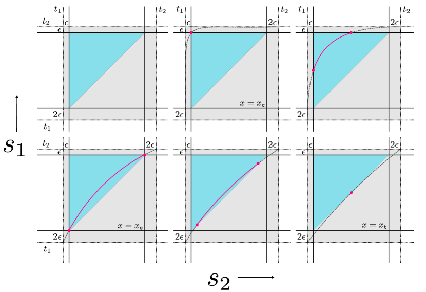
Figure 5: The integration range in the $(s_{1},s_{2})$ plane, (137), is denoted by the shaded upper triangular region in blue. For a given fixed value of the cross ratio $x$, $(s_{1},s_{2})$ trace a curve ${\cal C}_{x}$, denoted by the pink arcs in the panels above. The intersection points of ${\cal C}_{x}$ with the triangular region (137) determine the limits of the $s_{1}$ integral for fixed $x$, and are denoted by pink circles.

The original integration domain for $s_{1}$ and $s_{2}$ is the triangular region given by

$$s_{1}\in[t_{1}+\epsilon,t_{2}-2\epsilon]\;,\quad\text{and}\quad s_{2}\in[t_{1}+2\epsilon,t_{2}-\epsilon]\;,\quad\text{with}\quad s_{2}>s_{1}+\epsilon\;,$$ (137)

see figure 5. In the new variables $\{s_{1},x\}$, this region (137) is charted in a rather non-trivial way. We will do first the $s_{1}$-integration, so we need the range in $s_{1}$ for fixed $x$. In figure 5, we depict the curve ${\cal C}_{x}$ in the $(s_{1},s_{2})$ plane given by $s_{2}=s_{2}(x,s_{1})$. The integration limits for $s_{1}$ are the projections on the $s_{1}$-axis of the two points where ${\cal C}_{x}$ enters and exits the triangular integration region (137).

Depending on the values of $x$, $\mathcal{C}_{x}$ intersects the boundaries of the triangle on different sides (or lie completely outside of it). Accordingly, we need to split the $(x,s_{1})$ integration in the following way (cf. figure 5):

• Region 1: Here, $x_{\tt c}\leq x\leq x_{\tt e}$. The point $x=x_{\tt c}$ is the point such that ${\cal C}_{x}$ intersects the upper-left corner of the triangle, $(s_{1},s_{2})=(t_{1}+\epsilon,t_{2}-\epsilon)$, while $x_{\tt e}$ is the point where ${\cal C}_{x}$ intersects the lower-left corner of the triangle $(s_{1},s_{2})=(t_{1}+\epsilon,t_{2}+2\epsilon)$. In this range, ${\cal C}_{x}$ enters the triangle through its left side and exits through the top side.

• Region 2: Here, $x_{\tt e}\leq x\leq x_{\tt t}$, where $x_{\tt e}$ is defined as above and $x_{\tt t}$ is the point where ${\cal C}_{x}$ is tangent to the line $s_{2}=s_{1}+\epsilon$. In this range, ${\cal C}_{x}$ enters and exits the triangle through the diagonal side.

The values of $x_{\tt t}$, $x_{\tt e}$, $x_{\tt c}$ are easy to obtain explicitly. We will need only their expansion for small $\epsilon$:

$$x_{\tt c} = \frac{\epsilon^{2}}{2-2\cos\left(t_{1}-t_{2}\right)}+O\left(\epsilon^{3}\right)\sim 0\;,$$ (138)

$$x_{\tt e} = \frac{1}{2}+\frac{\epsilon}{4}\left(\cot\frac{t_{1}-t_{2}}{2}\right)+\frac{\epsilon^{2}}{4\cos\left(t_{1}-t_{2}\right)-4}+{\rm O}\left(\epsilon^{3}\right)\;\sim\frac{1}{2},$$ (139)

$$x_{\tt t} = 1+\epsilon\left(\cot\frac{t_{1}-t_{2}}{4}\right)+\frac{\epsilon^{2}}{2}\left(\cot^{2}\frac{t_{1}-t_{2}}{4}\right)+{\rm O}\left(\epsilon^{3}\right)\;\sim 1.$$ (140)

The region of integration is thus split naturally in two. For $x_{\tt c}\leq x\leq x_{\tt e}$ (Region 1), we have $s\in[\check{s}_{\tt i},\check{s}_{\tt f}]$, where $\check{s}_{\tt i}$ and $\check{s}_{\tt f}$ are given by the intersection points of ${\cal C}_{x}$, with the lines $s_{1}=t_{1}+\epsilon$ and $s_{2}=t_{2}-\epsilon$, respectively. These are given by

$$\check{s}_{\tt i} =t_{1}-\epsilon\;,$$ (141)

$$\check{s}_{\tt f} =t_{2}-\frac{\epsilon}{x}+\epsilon^{2}\left(\frac{x-1}{2\,x^{2}}\cot\frac{t_{1}-t_{2}}{2}\right)+{\rm O}\left(\epsilon^{3}\right)\;.$$ (142)

For $x_{\tt e}\leq x\leq x_{\tt t}$ (Region 2), we have $s_{1}\in[\hat{s}_{\tt i},\hat{s}_{\tt f}]$, with these points defined by the intersections of ${\cal C}_{x}$, with the line $s_{2}=s_{1}+\epsilon$. These are given by

$$\hat{s}_{\tt i}=t_{1}+\epsilon\left(\frac{x}{1-x}\right)-\epsilon^{2}\left({\frac{x}{2\,(x-1)^{2}}}\cot\frac{t_{1}-t_{2}}{2}\right)+{\rm O}(\epsilon^{3})\;,$$ (143)

$$\hat{s}_{\tt f}=t_{2}+\epsilon\left(\frac{1}{x-1}\right)+\epsilon^{2}\left(\frac{x}{2\,(x-1)^{2}}\cot\frac{t_{1}-t_{2}}{2}\right)+{\rm O}(\epsilon^{3})\;.$$ (144)

Putting all together, the original integration over the domain (137) rewrites as

$$\int_{t_{1}+2\epsilon}^{t_{2}-\epsilon}ds_{2}\int_{t_{1}+\epsilon}^{s_{2}-\epsilon}ds_{1}=\left[\int_{x_{\tt e}}^{x_{\tt t}}dx\int_{\hat{s}_{\tt i}}^{\hat{s}_{\tt f}}ds_{1}{\cal J}(s_{1},x)\right]+\left[\int_{x_{\tt c}}^{x_{\tt e}}dx\int_{\check{s}_{\tt i}}^{\check{s}_{\tt f}}ds_{1}{\cal J}(s_{1},x)\right]\;,$$ (145)

where ${\cal J}(s_{1},x)$ is the Jacobian of the transformation, given by

$${\cal J}(s_{1},x) = \left|\frac{\partial s_{2}(s_{1},x)}{\partial x}\right|$$

$$= -\frac{\sin\left(s_{1}-t_{1}\right)-\sin\left(s_{1}-t_{2}\right)+\sin\left(t_{1}-t_{2}\right)}{(x-1)\left(x\cos\left(s_{1}-t_{2}\right)-\cos\left(s_{1}-t_{1}\right)\right)+x\cos\left(t_{1}-t_{2}\right)-x^{2}+x-1}\;.$$

Armed with this change of variables formula, we are now able to simplify the various four-point integrals in (C.1). Notice that the expressions for $x_{\tt c}$, $x_{\tt e}$ and $x_{\tt t}$ go to $0$, $1/2$ and $1$ respectively, as $\epsilon\to 0$. As we compute the various integrals that enter (C.1) in the small-$\epsilon$ limit, these values will naturally appear as limits on the $x$-integration.

Let us list the result for the three terms in (C.1). Starting from the third line, after removing the tree-level part, we get the integral

$$\int_{t_{1}+2\epsilon}^{t_{2}-\epsilon}ds_{2}\int_{t_{1}+\epsilon}^{s_{2}-\epsilon}ds_{1}\,\delta G_{3}(t_{1},s_{1},s_{2},t_{2})\;{\rm P}(t_{1},s_{1})\;{\rm P}(t_{2},s_{2}).$$

Reverting to the $(x,s_{1})$ coordinates and doing the $s_{1}$ integration, the finite and divergent parts are

$$\int_{t_{1}+2\epsilon}^{t_{2}-\epsilon}ds_{2}\int_{t_{1}+\epsilon}^{s_{2}-\epsilon}ds_{1}\,\delta G_{3}(t_{1},s_{1},s_{2},t_{2})\;{\rm P}(t_{1},s_{1})\;{\rm P}(t_{2},s_{2})$$ (147)

$$={\rm P}(t_{1},t_{2})\left[\int_{0}^{\frac{1}{2}}dx\frac{\delta G_{3}(x)}{x^{2}}\;\log\left(\frac{x}{{\epsilon}^{2}\;{\rm P}(t_{1},t_{2})}\right)-\int_{\frac{1}{2}}^{1}dx\frac{\delta G_{3}(x)}{x^{2}}\;\log\left(\frac{x\epsilon^{2}{\rm P}(t_{1},t_{2})}{(x-1)^{2}}\right)\right]+{\rm O}(\epsilon)\;.$$

With the same method we evaluate the integral in the second line of (C.1), after subtracting the tree level contribution. This gives

$$\int_{t_{1}+\epsilon}^{t_{2}-\epsilon}ds_{1}\int_{t_{2}+\epsilon}^{t_{1}+2\pi-\epsilon}ds_{2}\,\delta G_{2}(t_{1},s_{1},t_{2},s_{2})\;{\rm P}(t_{1},s_{1})\;{\rm P}(t_{2},s_{2})$$ (148)

$$={\rm P}(t_{1},t_{2})\left[\int_{0}^{\frac{1}{2}}dx\frac{\delta G_{2}(x)}{x^{2}}\;\log\left(\frac{x{\epsilon}^{2}\;{\rm P}(t_{1},t_{2})}{1-x}\right)-\int_{\frac{1}{2}}^{1}dx\frac{\delta G_{2}(x)}{x^{2}}\;\log\left(\frac{x{\epsilon}^{2}\;{\rm P}(t_{1},t_{2})}{1-x}\right)\right]+{\rm O}(\epsilon)\;,$$

while the integrals coming from the first line of (C.1) evaluate to

$$\int_{t_{2}+2\epsilon}^{t_{1}+2\pi-\epsilon}ds_{2}\int_{t_{2}+\epsilon}^{s_{2}-\epsilon}ds_{1}\,\delta G_{1}(t_{1},t_{2},s_{1},s_{2})\;{\rm P}(t_{1},t_{2})\;{\rm P}(s_{2},s_{1})$$ (149)

$$={\rm P}(t_{1},t_{2})\left[\int_{0}^{\frac{1}{2}}dx\frac{\delta G_{1}(x)}{x^{2}}\;\log\left(\frac{x^{2}}{(1-x){\epsilon}^{2}\;{\rm P}(t_{1},t_{2})}\right)+\int_{\frac{1}{2}}^{1}dx\frac{\delta G_{1}(x)}{x^{2}}\;\log\left(\frac{1-x}{{\epsilon}^{2}{\rm P}(t_{1},t_{2})}\right)\right]+{\rm O}(\epsilon)\;.$$

So in total, summing (147)-(149), we have

Loops $$=\left[-\log\left(\epsilon^{2}{\rm P}(t_{1},t_{2})\right)\right]\,{\rm P}(t_{1},t_{2})$$ (150)

$$\!\!\!\!\!+\int_{0}^{\frac{1}{2}}\!\!dx\left[\frac{\delta G_{3}(x)}{x^{2}}\log{x}+\frac{\delta G_{1}(x)}{x^{2}}\log\!{\left(\!\frac{x^{2}}{1-x}\!\right)}+\frac{\delta G_{2}(x)}{x^{2}}\log\!{\left(\!\frac{x}{1-x}\!\right)}\right]\!{\rm P}(t_{1},t_{2})+{\rm O}(\epsilon)\;,$$

where we now used the crossing properties of the $G_{i}(x)$ amplitudes to map all the $x$ integrations to the interval $[0,\frac{1}{2}]$. Altogether, therefore we find

$$\mathcal{I}_{4-\text{pt}}=(2\mathbb{B})^{2}\frac{2\pi-6\epsilon}{\epsilon}{\rm P}(t_{1},t_{2})$$ (151)

$$+(2\mathbb{B})^{2}\int_{0}^{\frac{1}{2}}\!\!dx\left[\frac{\delta G_{3}(x)}{x^{2}}\log{x}+\frac{\delta G_{1}(x)}{x^{2}}\log\!{\left(\!\frac{x^{2}}{1-x}\!\right)}+\frac{\delta G_{2}(x)}{x^{2}}\log\!{\left(\!\frac{x}{1-x}\!\right)}\right]\!{\rm P}(t_{1},t_{2})+{\rm O}(\epsilon)\;.$$

Using these explicit integrals, the constraint (4.2) in the main text becomes the the sum-rule (78).

C.2 Integrals on the segment

We now discuss the explicit integrals entering the derivation in section 4.3.

Integrated 3-point function.

The first integral to compute is the 3-point contribution (121), we display it below for convenience:

$$\partial_{t_{1}}\partial_{t_{2}}L_{O_{n}}^{\text{3-pt}}=-b_{n,2}\epsilon^{\Delta_{n}-1}\int_{t_{1}+2\epsilon}^{t_{2}-2\epsilon}ds_{2}\bigg{[}\langle O_{\Phi_{\perp}^{1}}(t_{1}+\epsilon)O_{\Phi_{\perp}^{1}}(s_{2})O_{n}(t_{2}-\epsilon)\rangle_{1{\rm D}}\\ +\langle O_{\Phi_{\perp}^{1}}(t_{1}+\epsilon)O_{n}(s_{2})O_{\Phi_{\perp}^{1}}(t_{2}-\epsilon)\rangle_{1{\rm D}}+\langle O_{n}(t_{1}+\epsilon)O_{\Phi_{\perp}^{1}}(s_{2})O_{\Phi_{\perp}^{1}}(t_{2}-\epsilon)\rangle_{1{\rm D}}\bigg{]}\;.$$ (152)

It is a sum of three terms. The individual integrals are computed below. The first term of (152), gives

$$\epsilon^{\Delta_{n}-1}\int_{t_{1}+2\epsilon}^{t_{2}-2\epsilon}d\,s_{2}\,{\rm P}(t_{1}+\epsilon,s_{2})^{1-\frac{\Delta_{1}}{2}}\,{\rm P}(s_{2},t_{2}-\epsilon)^{\frac{\Delta_{1}}{2}}\,{\rm P}(t_{1}+\epsilon,t_{2}-\epsilon)^{\frac{\Delta_{1}}{2}}\\ =\frac{1}{\Delta_{n}-1}{\rm P}(t_{1}+\epsilon,t_{2}-\epsilon)+\mathcal{O}\left(\epsilon^{2\Delta_{n}-2}\right)\;.$$ (153)

The second term of (152), gives

$$\epsilon^{\Delta_{n}-1}\int_{t_{1}+2\epsilon}^{t_{2}-2\epsilon}d\,s_{2}\,{\rm P}(t_{1}+\epsilon,s_{2})^{\frac{\Delta_{1}}{2}}\,{\rm P}(s_{2},t_{2}-\epsilon)^{\frac{\Delta_{1}}{2}}\,{\rm P}(t_{1}+\epsilon,t_{2}-\epsilon)^{1-\frac{\Delta_{1}}{2}}\\ =\frac{2}{\Delta_{n}-1}{\rm P}(t_{1}+\epsilon,t_{2}-\epsilon)+\mathcal{O}\left(\epsilon^{2\Delta_{n}-2}\right)\;,$$ (154)

while the third term gives

$$\epsilon^{\Delta_{n}-1}\int_{t_{1}+2\epsilon}^{t_{2}-2\epsilon}d\,s_{2}\,{\rm P}(t_{1}+\epsilon,s_{2})^{\frac{\Delta_{1}}{2}}\,{\rm P}(s_{2},t_{2}-\epsilon)^{1-\frac{\Delta_{1}}{2}}\,{\rm P}(t_{1}+\epsilon,t_{2}-\epsilon)^{\frac{\Delta_{1}}{2}}\\ =\frac{1}{\Delta_{n}-1}{\rm P}(t_{1}+\epsilon,t_{2}-\epsilon)+\mathcal{O}\left(\epsilon^{2\Delta_{n}-2}\right)\;.$$ (155)

For their combination, we get

$$\partial_{t_{1}}\partial_{t_{2}}L_{O_{n}}^{\text{3-pt}}=-(2\mathbb{B})\,b_{n,2}\epsilon^{\Delta_{n}-1}\frac{4\,C_{n}}{\Delta_{n}-1}\,{\rm P}(t_{1}+\epsilon,t_{2}-\epsilon)\;.$$ (156)

Integrated 4-point function.

Our starting point is the integral (123), which we repeat below for convenience

$$\partial_{t_{1}}\partial_{t_{2}}L^{\text{4-pt}}\equiv-\int_{t_{1}+3\epsilon}^{t_{2}-2\epsilon}ds_{3}\int_{t_{1}+2\epsilon}^{s_{3}-\epsilon}ds_{2}\langle O_{\Phi_{\perp}^{1}}(t_{1}+\epsilon)O_{\Phi_{\perp}^{1}}(s_{2})O_{\Phi_{\perp}^{1}}(s_{3})O_{\Phi_{\perp}^{1}}(t_{2}-\epsilon)\rangle_{1{\rm D}}\;.$$

More explicitly, we have

$$\partial_{t_{1}}\partial_{t_{2}}L^{\text{4-pt}}\equiv-(2\mathbb{B})^{2}\;\int_{t_{1}+3\epsilon}^{t_{2}-2\epsilon}ds_{3}\int_{t_{1}+2\epsilon}^{s_{3}-\epsilon}ds_{2}\;{G(x)}\;{\rm P}({t}_{1}+\epsilon,s_{3})\,{\rm P}({t}_{2}-\epsilon,s_{2})\;,$$ (157)

Again it is convenient to separate the contribution of the tree level part (which is divergent). Moreover it is convenient on top of the tree level part to also include and subtract an extra pice. This piece corresponds to the non-planar diagram shown last in the second line in Figure 6. Namely, we define

$$\partial_{t_{1}}\partial_{t_{2}}L^{\text{4-pt}}\equiv(2\mathbb{B})^{2}\times\left(\texttt{Tree}^{\prime}+\texttt{Loops}^{\prime}\right),$$ (158)

where

$$\texttt{Loops}^{\prime}\equiv-\int_{t_{1}+3\epsilon}^{t_{2}-2\epsilon}ds_{3}\int_{t_{1}+2\epsilon}^{s_{3}-\epsilon}ds_{2}\;\left({\delta G(x)-x^{2}}\right)\;{\rm P}(t_{1}+\epsilon,s_{2})\,{\rm P}(t_{2}-\epsilon,s_{3})\;,$$ (159)

and

$$\texttt{Tree}^{\prime}\equiv-\int_{t_{1}+3\epsilon}^{t_{2}-2\epsilon}ds_{3}\int_{t_{1}+2\epsilon}^{s_{3}-\epsilon}ds_{2}\;\left({G_{\text{tree}}(x)+x^{2}}\right)\;{\rm P}(t_{1}+\epsilon,s_{2})\,{\rm P}(t_{2}-\epsilon,s_{3})\;.$$ (160)

The extra $x^{2}$ term is particularly convenient to recombine $\texttt{Tree}^{\prime}$ with another contribution, as we will see shortly.

The most complicated part can be computed by the same method illustrated in the previous section, i.e. we trade one of the integration variables for an integral over the cross ratio $x$ defined by (135). This results in

$$\texttt{Loops}^{\prime} =-{\rm P}(t_{1},t_{2})\,\left(\int_{0}^{\frac{1}{2}}dx\,\frac{\delta G(x)-x^{2}}{x^{2}}\log{\left(\frac{x^{3}}{1-x}\right)}\right)+\mathcal{O}(\epsilon)$$

$$=-{\rm P}(t_{1},t_{2})\,\left(-\int_{0}^{\frac{1}{2}}dx\,\log{\left(\frac{x^{3}}{1-x}\right)}+\int_{0}^{\frac{1}{2}}dx\,\frac{\delta G(x)}{x^{2}}\log{\left(\frac{x^{3}}{1-x}\right)}\right)+\mathcal{O}(\epsilon)$$

$$=-{\rm P}(t_{1},t_{2})\,\left(1+\log 4+\int_{0}^{\frac{1}{2}}dx\,\frac{\delta G(x)}{x^{2}}\log{\left(\frac{x^{3}}{1-x}\right)}\right)+\mathcal{O}(\epsilon)\;.$$ (161)

The tree level part is defined explicitly as

$$\texttt{Tree}^{\prime}\equiv-\int_{t_{1}+3\epsilon}^{t_{2}-2\epsilon}ds_{3}\int_{t_{1}+2\epsilon}^{s_{3}-\epsilon}ds_{2}\;\left[{\rm P}(t_{1}+\epsilon,s_{1})\,{\rm P}(t_{2}-\epsilon,s_{2})\right.\\ \left.+{\rm P}(t_{1}+\epsilon,{{t}}_{2}-\epsilon)\,{\rm P}(s_{1},s_{2})+{\rm P}(t_{1}+\epsilon,s_{2})\,{\rm P}(t_{2}-\epsilon,s_{1})\right]\;.$$ (162)

This contribution can be evaluated explicitly with Mathematica and then expanded in the cutoffs. It is a complicated and divergent expression, however all divergences are cancelled by other terms coming from the expansion of $-\frac{1}{2}\partial_{t_{1}}\partial_{t_{2}}A^{2}(t_{1},t_{2})$ defined in (112). What will be relevant for us is the combination:

$$\texttt{Tree}^{\prime}-\underbrace{\frac{1}{2}\partial_{t_{1}}\partial_{t_{2}}\left[\int_{t_{1}+\epsilon}^{t_{2}-2\epsilon}ds_{2}\int_{s_{2}+\epsilon}^{t_{2}-\epsilon}ds_{3}\,{\rm P}(s_{2},s_{3})\right]^{2}}_{\equiv\texttt{Subtraction}},$$ (163)

where the second term comes from $-\frac{1}{2}\partial_{t_{1}}\partial_{t_{2}}[K^{\texttt{2-pt}}]^{2}\equiv-(2\mathbb{B})^{2}\,(\texttt{Subtraction})$ in (112), and can be rewritten as

$$\texttt{Subtraction}=-{\rm P}(t_{1}+{\epsilon},t_{2}-{\epsilon})\;\int_{t_{1}+\epsilon}^{t_{2}-2\epsilon}ds_{2}\int_{s_{2}+\epsilon}^{t_{2}-\epsilon}ds_{3}\,{\rm P}(s_{2},s_{3})$$ (164)

$$-\left(\int_{t_{1}+2\epsilon<s_{2}<t_{2}-{\epsilon}}{ds_{2}}\,{\rm P}(t_{1}+\epsilon,s_{2})\right)\times\left(\int_{t_{1}+{\epsilon}<s_{3}<t_{2}-2\epsilon}{ds_{3}}\,{\rm P}(t_{2}-\epsilon,s_{3})\right).$$

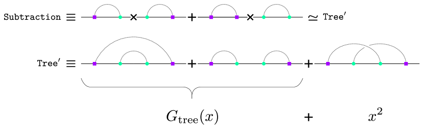
Figure 6: Here we illustrate schematically some terms appearing in the calculation (with purple squares $\simeq$ fixed variables, and green circles $\simeq$ integrated variables). The term Tree^′ is given by the tree-level 4-point function, integrated in the two middle variables, plus an extra term given by two propagators crossed in a non-planar fashion. Superficially, these terms have the same form as the terms of the Subtraction, which are also given in the first line in terms of products of integrated 2-point functions integrated in some of the variables. The only mismatch comes from the range of the integrated variables, cf. (162) vs (164). The tiny $\epsilon$-dependent mismatch, combined with the divergence of the integrals, produces a finite result in our calculation, cf. (165).

As can be seen most easily graphically, see Figure 6, the combination $\texttt{Tree}^{\prime}-\texttt{Subtraction}$ almost perfectly cancels. Notice however that the integration regions are slightly different, by an infinitesimal amount. This combines with the divergences of the integrals to give a finite result for the difference. Evaluating the integrals explicitly, we can compute

$$\texttt{Tree}^{\prime}-\texttt{Subtraction}={\rm P}(t_{1},t_{2})\;\left(6+\log{4}\right)+\mathcal{O}(\epsilon).$$ (165)

All in all we have a finite result

$$\partial_{t_{1}}\partial_{t_{2}}L^{\text{4-pt}}-\frac{1}{2}\partial_{t_{1}}\partial_{t_{2}}[K^{\texttt{2-pt}}]^{2}=(2\mathbb{B})^{2}\;\left(\texttt{Tree}^{\prime}+\texttt{Loops}^{\prime}-\texttt{Subtraction}\right)$$ (166)

$$= -(2\mathbb{B})^{2}\,{\rm P}(t_{1},t_{2})\,\left(-5+\int_{0}^{\frac{1}{2}}dx\frac{\delta G(x)}{x^{2}}\log{\left(\frac{x^{3}}{1-x}\right)}\right)\;.$$

Appendix D Normalisation of $\Phi_{||}$: details

Weak coupling.

The anomalous term in (79) arise from the divergence of the superconformal block of the long-multiplet at $x\sim 0$ for $\Delta_{1}=1$. The divergent contribution is given by the following integral

$$\int_{\delta_{x}}^{1/2}\frac{x-2}{1-\Delta_{1}}x^{\Delta_{1}-2}dx\;.$$ (167)

At finite coupling $\Delta_{1}>1$, the integral is convergent and it gives

$$I_{\text{finite}}=\frac{2^{-\Delta_{1}}(3\Delta_{1}+1)}{(\Delta_{1}-1)^{2}\Delta_{1}}\;.$$ (168)

At weak coupling $\Delta_{1}=1+\gamma_{1}$, we expand first for small $\gamma_{1}$ and then integrate. Choosing the prescription in which $\log\delta_{x}\rightarrow 0$, we can resum order by order in $\gamma_{1}$ obtaining

$$I_{\text{weak}} =\frac{1}{2(\Delta_{1}\!-\!1)}+\sum_{k=1}^{\infty}\biggl{[}\frac{(1-\Delta_{1})^{k-1}}{2}\left(\!1+\frac{4\log^{k}2}{(1-\Delta_{1})k!}\right)\!+\frac{\log^{k}2}{2k!}\!\!\sum_{n=k-1}^{\infty}\!(1-\Delta_{1})^{n}\biggl{]}$$

$$=\frac{2^{-\Delta_{1}}\left(1-\left(2^{\Delta_{1}+1}-3\right)\Delta_{1}\right)}{(\Delta_{1}-1)^{2}\Delta_{1}}\;.$$ (169)

The anomaly is proportional to the discrepancy of the two previous results

$$\delta I=I_{\text{finite}}-I_{\text{weak}}=\frac{2}{(\Delta_{1}-1)^{2}}\;.$$ (170)

Since the integral (167) comes from the OPE, it is multiplied by $C_{1}^{2}$ leading to the following identity

$$\left.\int_{\delta_{x}}^{1/2}\!\frac{(x-2)\delta f(x)}{x^{3}}\;dx\right|_{\text{small }g}\!\!\!\!\sim\underbrace{\int_{\delta_{x}}^{\frac{1}{2}}dx\frac{(x-2)\sum_{\ell=1}^{M}g^{2\ell}f_{\text{weak}}^{(\ell)}(x)}{x^{3}}}_{\texttt{regularised, }\log(\delta_{x})\rightarrow 0}+\underbrace{\left[\frac{2\;C_{1}^{2}}{(\Delta_{1}-1)^{2}}\right]}_{\texttt{``anomaly''}}+\mathcal{O}(g^{2M+2}),$$ (171)

where $f_{\text{weak}}^{(\ell)}(x)$ is the weak coupling reduced correlator at $\ell$ loops given in Cavaglia:2022qpg together with the perturbative expansions of $C_{1}^{2}$ and $\Delta_{1}$.

Using equation (171) together with (79), we can compute the Wilson coefficient $b_{1,2}$ up to order $g^{7}$, obtaining the following expansion

$$b_{1,2} =\frac{g}{\sqrt{2}}-\frac{g^{3}\left(\pi^{2}-6\right)}{3\sqrt{2}}+\frac{g^{5}\left(-108(\zeta_{3}+3)+12\pi^{2}+5\pi^{4}+576\log 2\right)}{18\sqrt{2}}$$

$$+\frac{g^{7}}{270\sqrt{2}}\biggl{[}60\pi^{2}\left(132\zeta_{3}+399+8\log^{3}2-8(36+3\log 2)\log 2\right)-71\pi^{6}-138915\zeta_{5}$$

$$+6\pi^{4}(91-188\log 2)-72\biggl{(}-15\left(32\text{Li}_{4}\left(\tfrac{1}{2}\right)-16\text{Li}_{5}\left(\tfrac{1}{2}\right)+16S_{3,2}\left(\tfrac{1}{2}\right)+33\zeta_{3}-271\right)$$

$$+60\log 2\left(4\text{Li}_{4}\left(\tfrac{1}{2}\right)+\zeta_{3}(2\log 2-7)-4\right)+(6\log 2-20)\log^{4}2\biggl{)}\biggl{]}+\,\mathcal{O}\left(g^{9}\right)\;,$$ (172)

where $\text{Li}_{n}(x)$ are polylogarithms and $S_{n,m}(x)$ are Nielsen generalised polylogarithms (or hyperlogarithm).

Strong coupling.

At strong coupling we obtain the following expansion

$$b_{1,2}=\frac{g(1\!+\!\log 2)}{\sqrt{2/5}\,\pi}-\frac{149\!-\!8\pi^{2}\!+\!17\log 2}{96\,\sqrt{2/5}\,\pi^{2}}+\frac{5616\zeta_{3}\!+\!21003\!-\!1232\pi^{2}\!+\!45\log 2(256\log 2\!-\!129)}{18432\,\sqrt{2/5}\,\pi^{3}g}$$

$$+\frac{477631\log 2\!-\!864\zeta_{3}(515\!+\!76\log 2)\!-\!1039805\!+\!65496\pi^{2}\!+\!2304\log^{2}2(216\log 2\!-\!673)}{1769472\,\sqrt{2/5}\,\pi^{4}g^{2}}$$

$$+\frac{1}{679477248\sqrt{10}\pi^{5}g^{3}}\biggl{[}5\biggl{(}53747712\text{Li}_{5}\left(\tfrac{1}{2}\right)-71663616S_{3,2}\left(\tfrac{1}{2}\right)+183253536\zeta_{3}+8024832\zeta_{5}$$

$$+223558211-96292333\log 2\biggl{)}+32\biggl{(}108\log 2(77760\text{Li}_{4}\left(\tfrac{1}{2}\right)+204295\zeta_{3}+4\log 2(14850\zeta_{3}$$

$$+\!175355\!+\!16\log 2(\log 2(2890\!+\!27\log 2)\!-\!10480)))\!-\!5\pi^{2}\left(324864\zeta_{3}\!+\!420965+46656\log^{3}2\right)$$

$$-15552\pi^{4}\log 2\biggl{)}\biggl{]}+\,\mathcal{O}\left(\frac{1}{g^{4}}\right)\;.$$ (173)

References

- (1) A. Cavaglià, N. Gromov, J. Julius, and M. Preti, Integrability and conformal bootstrap: One dimensional defect conformal field theory, Phys. Rev. D 105 (2022), no. 2 L021902, [arXiv:2107.08510].
- (2) A. Cavaglià, N. Gromov, J. Julius, and M. Preti, Bootstrability in Defect CFT: Integrated Correlators and Sharper Bounds, arXiv:2203.09556.
- (3) S. Caron-Huot, F. Coronado, A.-K. Trinh, and Z. Zahraee, Bootstrapping sYM correlators using integrability, arXiv:2207.01615.
- (4) N. Gromov, V. Kazakov, S. Leurent, and D. Volin, Quantum Spectral Curve for Planar Super-Yang-Mills Theory, Phys. Rev. Lett. 112 (2014), no. 1 011602, [arXiv:1305.1939].
- (5) N. Gromov, V. Kazakov, S. Leurent, and D. Volin, Quantum spectral curve for arbitrary state/operator in AdS5/CFT4, JHEP 09 (2015) 187, [arXiv:1405.4857].
- (6) R. Rattazzi, V. S. Rychkov, E. Tonni, and A. Vichi, Bounding scalar operator dimensions in 4D CFT, JHEP 12 (2008) 031, [arXiv:0807.0004].
- (7) S. El-Showk, M. F. Paulos, D. Poland, S. Rychkov, D. Simmons-Duffin, and A. Vichi, Solving the 3D Ising Model with the Conformal Bootstrap, Phys. Rev. D 86 (2012) 025022, [arXiv:1203.6064].
- (8) D. Poland, S. Rychkov, and A. Vichi, The Conformal Bootstrap: Theory, Numerical Techniques, and Applications, Rev. Mod. Phys. 91 (2019) 015002, [arXiv:1805.04405].
- (9) S. M. Chester, “Weizmann Lectures on the Numerical Conformal Bootstrap.” 7, 2019.
- (10) N. B. Agmon, S. M. Chester, and S. S. Pufu, Solving M-theory with the Conformal Bootstrap, JHEP 06 (2018) 159, [arXiv:1711.07343].
- (11) C. Beem, L. Rastelli, and B. C. van Rees, The Superconformal Bootstrap, Phys. Rev. Lett. 111 (2013) 071601, [arXiv:1304.1803].
- (12) C. Beem, L. Rastelli, and B. C. van Rees, More superconformal bootstrap, Phys. Rev. D 96 (2017), no. 4 046014, [arXiv:1612.02363].
- (13) S. M. Chester, R. Dempsey, and S. S. Pufu, Bootstrapping super-Yang-Mills on the conformal manifold, arXiv:2111.07989.
- (14) O. Aharony, L. F. Alday, A. Bissi, and E. Perlmutter, Loops in AdS from Conformal Field Theory, JHEP 07 (2017) 036, [arXiv:1612.03891].
- (15) L. F. Alday and A. Bissi, Loop Corrections to Supergravity on , Phys. Rev. Lett. 119 (2017), no. 17 171601, [arXiv:1706.02388].
- (16) L. F. Alday, T. Hansen, and J. A. Silva, AdS Virasoro-Shapiro from dispersive sum rules, JHEP 10 (2022) 036, [arXiv:2204.07542].
- (17) L. F. Alday, T. Hansen, and J. A. Silva, AdS Virasoro-Shapiro from single-valued periods, arXiv:2209.06223.
- (18) N. Kiryu and S. Komatsu, Correlation Functions on the Half-BPS Wilson Loop: Perturbation and Hexagonalization, JHEP 02 (2019) 090, [arXiv:1812.04593].
- (19) P. Ferrero and C. Meneghelli, Bootstrapping the half-BPS line defect CFT in N=4 supersymmetric Yang-Mills theory at strong coupling, Phys. Rev. D 104 (2021), no. 8 L081703, [arXiv:2103.10440].
- (20) D. J. Binder, S. M. Chester, S. S. Pufu, and Y. Wang, = 4 Super-Yang-Mills correlators at strong coupling from string theory and localization, JHEP 12 (2019) 119, [arXiv:1902.06263].
- (21) H. Paul, E. Perlmutter, and H. Raj, Integrated Correlators in SYM via Spectral Theory, arXiv:2209.06639.
- (22) D. Dorigoni, M. B. Green, and C. Wen, Novel Representation of an Integrated Correlator in = 4 Supersymmetric Yang-Mills Theory, Phys. Rev. Lett. 126 (2021), no. 16 161601, [arXiv:2102.08305].
- (23) D. Dorigoni, M. B. Green, and C. Wen, Exact properties of an integrated correlator in = 4 SU(N) SYM, JHEP 05 (2021) 089, [arXiv:2102.09537].
- (24) D. Dorigoni, M. B. Green, and C. Wen, Exact results for duality-covariant integrated correlators in SYM with general classical gauge groups, arXiv:2202.05784.
- (25) N. Drukker, Z. Kong, and G. Sakkas, Broken R-symmetry and defect conformal manifolds, arXiv:2203.17157.
- (26) J. Barrat, P. Liendo, G. Peveri, and J. Plefka, Multipoint correlators on the supersymmetric Wilson line defect CFT, arXiv:2112.10780.
- (27) J. Barrat, P. Liendo, and G. Peveri, Multipoint correlators on the supersymmetric Wilson line defect CFT II: Unprotected operators, arXiv:2210.14916.
- (28) J. M. Maldacena, Wilson loops in large N field theories, Phys. Rev. Lett. 80 (1998) 4859–4862, [hep-th/9803002].
- (29) N. Drukker and D. J. Gross, An Exact prediction of N=4 SUSYM theory for string theory, J. Math. Phys. 42 (2001) 2896–2914, [hep-th/0010274].
- (30) N. Drukker, D. J. Gross, and H. Ooguri, Wilson loops and minimal surfaces, Phys. Rev. D 60 (1999) 125006, [hep-th/9904191].
- (31) J. K. Erickson, G. W. Semenoff, and K. Zarembo, Wilson loops in N=4 supersymmetric Yang-Mills theory, Nucl. Phys. B582 (2000) 155–175, [hep-th/0003055].
- (32) K. Zarembo, Supersymmetric Wilson loops, Nucl. Phys. B 643 (2002) 157–171, [hep-th/0205160].
- (33) V. Pestun, Localization of the four-dimensional N=4 SYM to a two-sphere and 1/8 BPS Wilson loops, JHEP 12 (2012) 067, [arXiv:0906.0638].
- (34) M. Gunaydin and R. J. Scalise, Unitary Lowest Weight Representations of the Noncompact Supergroup Osp(2m*/2n), J. Math. Phys. 32 (1991) 599–606.
- (35) P. Liendo and C. Meneghelli, Bootstrap equations for = 4 SYM with defects, JHEP 01 (2017) 122, [arXiv:1608.05126].
- (36) P. Liendo, C. Meneghelli, and V. Mitev, Bootstrapping the half-BPS line defect, JHEP 10 (2018) 077, [arXiv:1806.01862].
- (37) S. Giombi, R. Roiban, and A. A. Tseytlin, Half-BPS Wilson loop and AdS2/CFT1, Nucl. Phys. B922 (2017) 499–527, [arXiv:1706.00756].
- (38) M. Cooke, A. Dekel, and N. Drukker, The Wilson loop CFT: Insertion dimensions and structure constants from wavy lines, J. Phys. A50 (2017), no. 33 335401, [arXiv:1703.03812].
- (39) D. Grabner, N. Gromov, and J. Julius, Excited States of One-Dimensional Defect CFTs from the Quantum Spectral Curve, JHEP 07 (2020) 042, [arXiv:2001.11039].
- (40) J. Julius, Modern techniques for solvable models. PhD thesis, King’s Coll. London, 2021.
- (41) N. B. Agmon and Y. Wang, Classifying Superconformal Defects in Diverse Dimensions Part I: Superconformal Lines, arXiv:2009.06650.
- (42) N. Drukker and S. Kawamoto, Small deformations of supersymmetric Wilson loops and open spin-chains, JHEP 07 (2006) 024, [hep-th/0604124].
- (43) A. M. Polyakov and V. S. Rychkov, Gauge field strings duality and the loop equation, Nucl. Phys. B 581 (2000) 116–134, [hep-th/0002106].
- (44) G. W. Semenoff and D. Young, Wavy Wilson line and AdS / CFT, Int. J. Mod. Phys. A 20 (2005) 2833–2846, [hep-th/0405288].
- (45) D. Correa, J. Henn, J. Maldacena, and A. Sever, An exact formula for the radiation of a moving quark in N=4 super Yang Mills, JHEP 06 (2012) 048, [arXiv:1202.4455].
- (46) A. Cavaglià, D. Grabner, N. Gromov, and A. Sever, Colour-Twist Operators I: Spectrum and Wave Functions, arXiv:2001.07259.
- (47) G. P. Korchemsky and A. V. Radyushkin, Loop Space Formalism and Renormalization Group for the Infrared Asymptotics of QCD, Phys. Lett. B 171 (1986) 459–467.
- (48) N. Drukker and V. Forini, Generalized quark-antiquark potential at weak and strong coupling, JHEP 06 (2011) 131, [arXiv:1105.5144].
- (49) D. Correa, J. Maldacena, and A. Sever, The quark anti-quark potential and the cusp anomalous dimension from a TBA equation, JHEP 08 (2012) 134, [arXiv:1203.1913].
- (50) N. Drukker, Integrable Wilson loops, JHEP 10 (2013) 135, [arXiv:1203.1617].
- (51) N. Gromov and F. Levkovich-Maslyuk, Quantum Spectral Curve for a cusped Wilson line in SYM, JHEP 04 (2016) 134, [arXiv:1510.02098].
- (52) B. Fiol, B. Garolera, and A. Lewkowycz, Exact results for static and radiative fields of a quark in N=4 super Yang-Mills, JHEP 05 (2012) 093, [arXiv:1202.5292].
- (53) N. Drukker, 1/4 BPS circular loops, unstable world-sheet instantons and the matrix model, JHEP 09 (2006) 004, [hep-th/0605151].
- (54) N. Gromov and A. Sever, Analytic Solution of Bremsstrahlung TBA, JHEP 11 (2012) 075, [arXiv:1207.5489].
- (55) N. Gromov, F. Levkovich-Maslyuk, and G. Sizov, Analytic Solution of Bremsstrahlung TBA II: Turning on the Sphere Angle, JHEP 10 (2013) 036, [arXiv:1305.1944].
- (56) G. Sizov and S. Valatka, Algebraic Curve for a Cusped Wilson Line, JHEP 05 (2014) 149, [arXiv:1306.2527].
- (57) M. Bonini, L. Griguolo, M. Preti, and D. Seminara, Bremsstrahlung function, leading Lüscher correction at weak coupling and localization, JHEP 02 (2016) 172, [arXiv:1511.05016].
- (58) A. Cavaglià, N. Gromov, and F. Levkovich-Maslyuk, Quantum spectral curve and structure constants in SYM: cusps in the ladder limit, JHEP 10 (2018) 060, [arXiv:1802.04237].
- (59) H. Dorn, On anomalous conformal Ward identities for Wilson loops on polygon-like contours with circular edges, arXiv:2001.03391.
- (60) J. L. Cardy, Scaling and renormalization in statistical physics. 1996.
- (61) A. B. Zamolodchikov, Renormalization Group and Perturbation Theory Near Fixed Points in Two-Dimensional Field Theory, Sov. J. Nucl. Phys. 46 (1987) 1090.
- (62) A. Zamolodchikov, Integrable field theory from conformal field theory, in Integrable Sys Quantum Field Theory (M. Jimbo, T. Miwa, and A. Tsuchiya, eds.), pp. 641–674. Academic Press, San Diego, 1989.
- (63) D. Kutasov, Geometry on the Space of Conformal Field Theories and Contact Terms, Phys. Lett. B 220 (1989) 153–158.
- (64) K. Ranganathan, H. Sonoda, and B. Zwiebach, Connections on the state space over conformal field theories, Nucl. Phys. B 414 (1994) 405–460, [hep-th/9304053].
- (65) M. R. Gaberdiel, A. Konechny, and C. Schmidt-Colinet, Conformal perturbation theory beyond the leading order, J. Phys. A 42 (2009) 105402, [arXiv:0811.3149].
- (66) A. Amoretti and N. Magnoli, Conformal perturbation theory, Phys. Rev. D 96 (2017), no. 4 045016, [arXiv:1705.03502].
- (67) C. Behan, Conformal manifolds: ODEs from OPEs, JHEP 03 (2018) 127, [arXiv:1709.03967].
- (68) M. Baggio, V. Niarchos, and K. Papadodimas, Aspects of Berry phase in QFT, JHEP 04 (2017) 062, [arXiv:1701.05587].
- (69) B. Gabai, A. Sever, and D.-l. Zhong, Line Operators in Chern-Simons–Matter Theories and Bosonization in Three Dimensions, Phys. Rev. Lett. 129 (2022), no. 12 121604, [arXiv:2204.05262].
- (70) D. Maitre, HPL, a mathematica implementation of the harmonic polylogarithms, Comput. Phys. Commun. 174 (2006) 222–240, [hep-ph/0507152].
- (71) L. Bianchi, L. Griguolo, M. Preti, and D. Seminara, Wilson lines as superconformal defects in ABJM theory: a formula for the emitted radiation, JHEP 10 (2017) 050, [arXiv:1706.06590].
- (72) L. Bianchi, M. Preti, and E. Vescovi, Exact Bremsstrahlung functions in ABJM theory, JHEP 07 (2018) 060, [arXiv:1802.07726].
- (73) L. Bianchi, G. Bliard, V. Forini, L. Griguolo, and D. Seminara, Analytic bootstrap and Witten diagrams for the ABJM Wilson line as defect CFT1, JHEP 08 (2020) 143, [arXiv:2004.07849].
- (74) N. Gorini, L. Griguolo, L. Guerrini, S. Penati, D. Seminara, and P. Soresina, Constant primary operators and where to find them: The strange case of BPS defects in ABJ(M) theory, arXiv:2209.11269.
- (75) L. Griguolo, D. Marmiroli, G. Martelloni, and D. Seminara, The generalized cusp in ABJ(M) N = 6 Super Chern-Simons theories, JHEP 05 (2013) 113, [arXiv:1208.5766].
- (76) M. Bonini, L. Griguolo, M. Preti, and D. Seminara, Surprises from the resummation of ladders in the ABJ(M) cusp anomalous dimension, JHEP 05 (2016) 180, [arXiv:1603.00541].
- (77) M. S. Bianchi, L. Griguolo, M. Leoni, S. Penati, and D. Seminara, BPS Wilson loops and Bremsstrahlung function in ABJ(M): a two loop analysis, JHEP 06 (2014) 123, [arXiv:1402.4128].
- (78) D. H. Correa, J. Aguilera-Damia, and G. A. Silva, Strings in Wilson loops in 6 super Chern-Simons-matter and bremsstrahlung functions, JHEP 06 (2014) 139, [arXiv:1405.1396].
- (79) M. S. Bianchi, L. Griguolo, A. Mauri, S. Penati, M. Preti, and D. Seminara, Towards the exact Bremsstrahlung function of ABJM theory, JHEP 08 (2017) 022, [arXiv:1705.10780].
- (80) N. Drukker et al., Roadmap on Wilson loops in 3d Chern–Simons-matter theories, J. Phys. A 53 (2020), no. 17 173001, [arXiv:1910.00588].
- (81) A. Cavaglià, D. Fioravanti, N. Gromov, and R. Tateo, Quantum Spectral Curve of the 6 Supersymmetric Chern-Simons Theory, Phys. Rev. Lett. 113 (2014), no. 2 021601, [arXiv:1403.1859].
- (82) D. Bombardelli, A. Cavaglià, D. Fioravanti, N. Gromov, and R. Tateo, The full Quantum Spectral Curve for , JHEP 09 (2017) 140, [arXiv:1701.00473].
- (83) J. K. Erickson, G. W. Semenoff, R. J. Szabo, and K. Zarembo, Static potential in N=4 supersymmetric Yang-Mills theory, Phys. Rev. D61 (2000) 105006, [hep-th/9911088].
- (84) A. B. Zamolodchikov, ’FISHNET’ DIAGRAMS AS A COMPLETELY INTEGRABLE SYSTEM, Phys. Lett. B 97 (1980) 63–66.
- (85) O. Gürdoğan and V. Kazakov, New Integrable 4D Quantum Field Theories from Strongly Deformed Planar 4 Supersymmetric Yang-Mills Theory, Phys. Rev. Lett. 117 (2016), no. 20 201602, [arXiv:1512.06704]. [Addendum: Phys.Rev.Lett. 117, 259903 (2016)].
- (86) J. a. Caetano, O. Gürdoğan, and V. Kazakov, Chiral limit of = 4 SYM and ABJM and integrable Feynman graphs, JHEP 03 (2018) 077, [arXiv:1612.05895].
- (87) V. Kazakov, E. Olivucci, and M. Preti, Generalized fishnets and exact four-point correlators in chiral CFT4, JHEP 06 (2019) 078, [arXiv:1901.00011].
- (88) A. Pittelli and M. Preti, Integrable fishnet from -deformed quivers, Phys. Lett. B 798 (2019) 134971, [arXiv:1906.03680].
- (89) N. Gromov, J. Julius, and N. Primi, Open fishchain in N = 4 Supersymmetric Yang-Mills Theory, JHEP 07 (2021), no. 127 127, [arXiv:2101.01232].