Collaborative Video Analytics on Distributed Edges with Multiagent Deep Reinforcement Learning

Abstract

Deep Neural Network (DNN) based video analytics empowers many computer vision-based applications to achieve high recognition accuracy. To reduce inference delay and bandwidth cost for video analytics, the DNN models can be deployed on the edge nodes, which are proximal to end users. However, the processing capacity of an edge node is limited, potentially incurring substantial delay if the inference requests on an edge node is overloaded. While efforts have been made to enhance the video analytics by optimizing the configurations on a single edge node, we observe that multiple edge nodes can work collaboratively by utilizing the idle resources on each other to improve the overall processing capacity and resource utilization. To this end, we propose a Multiagent Reinforcement Learning (MARL) based approach, named as EdgeVision, for collaborative video analytics on distributed edges. The edge nodes can jointly learn the optimal policies for video preprocessing, model selection, and request dispatching by collaborating with each other to minimize the overall cost. We design an actor-critic based MARL algorithm with an attention mechanism to learn the optimal policies. We build a multi-edge-node testbed and conduct the experiments with real-world datasets to evaluate the performance of our method. The experimental results show our method can improve the overall rewards by 33.6%-86.4% compared with the most competitive baseline methods.

I Introduction

Video analytics is widely adopted in many computer vision-based applications, such as video surveillance, augmented reality, autonomous driving, etc. Currently, most of the state-of-the-art video analytics algorithms are implemented with Deep Neural Networks (DNNs). The DNN-based video analytics can achieve high accuracy, however, deploying DNN models for video analytics faces many challenges in real-world scenarios [1]. The DNN models for video analytics usually consist of hundreds of layers, which are compute-intensive and may incur substantial delay for inference [2, 3]. Moreover, the volume of video content is large, transmitting raw video content to the cloud for inference may incur large bandwidth cost and intolerable transmission delay.

To reduce bandwidth cost and data transmission delay for video analytics applications, the DNN models can be deployed on edge nodes, which are proximal to the users [4, 5]. The edge nodes can receive video data from users with negligible delay. However, the processing capacity of an edge node is limited. When a large number of inference requests arrive, the edge node may be overloaded, exceeding its processing capacity and significantly increasing inference delay. Therefore, the video analytics mechanism with edge computing should be carefully designed to guarantee performance.

Some previous works have studied how to improve the performance of video analytics pipelines under the edge computing or cloud computing paradigm. For instance, Osmoticgate [6], SmartEye [7], DeepDecision [8], and FastVA [9] studied the offloading mechanism between the client and the edge node for video analytics. These works mainly focused on the adaptation of the video analytics configurations for video preprocessing and model selection on the edge and client to balance inference accuracy and delay. $A^{2}$ [2] and EdgeAdaptor [10] considered the selection of different versions of compressed DNN models for optimizing delay, accuracy, and service cost. Reducto [11], AppealNet [12], and ClodSeg [13] adopted frame filtering, inference difficulty classification, and resolution downsizing to reduce communication cost for video transmission while maintaining accuracy.

The previous efforts that studied video analytics pipelines under the edge computing paradigm mainly focused on the adaptation of video analytics configurations on one single edge node. However, the computational capacity of one edge node is scarce, which can easily lead to overload. Moreover, these edge nodes are located at different geographical regions, and the workloads of the edge nodes are time-varying and imbalanced [14]. The workloads of some edge nodes may be light, whereas others may be overloaded. Therefore, it is necessary to consider the collaboration of multiple edge nodes to improve the overall performance of the video analytics system.

It posits many challenges for optimizing the video analytic pipelines with edge collaboration. One edge node needs not only to consider its own workloads for the decision-making of video frame preprocessing and model selection, but also needs to consider the workloads and the decision-making of other edge nodes to maximize the overall performance. Therefore, the decision-making for the video analytics pipelines becomes more complex. Moreover, each edge node is an autonomous entity, which needs to work collaboratively with others while making its own decisions for the received inference requests. Therefore, a distributed decision-making mechanism is required to support the edge nodes to work collaboratively.

In this paper, we propose a Multiagent Reinforcement Learning (MARL) based approach for collaborative video analytics on distributed edge nodes. Multiple edge nodes can cooperate with each other by dynamically determining the selection of DNN models, video frame preprocessing configurations, and the edge node for inference, based on the workloads and the bandwidth conditions of the edge nodes. We model each edge node as an agent, which is an autonomous entity to make distributed control decisions by observing its local state. We design a MARL-based algorithm that enables the agents to learn collaboratively to maximize the overall system performance. The algorithm is featured by the attention mechanism that can differentiate the importance of information collected from the edge nodes. To evaluate the performance of our proposed method, we implement a video analytics testbed with multiple edge nodes and conduct extensive experiments using real-world datasets and experimental settings. The experimental results show that EdgeVision can significantly improve the reward by 33.6%-86.4% compared with the baseline methods. The main contributions of the paper are summarized as follows.

• Design a collaborative video analytics system in which the edge nodes can collaborate with each other for dynamically video prepossessing, model selection, and inference dispatching to maximize performance.

• Propose an attention-driven MARL approach for learning optimal policies. The agents of mulitple edge nodes can collaboratively learn the optimal policy by sharing their information to maximize the reward.

• Evaluate the performance of the proposed method with real-world datasets and verify the effectiveness under different practical settings. Our method can improve the overall rewards by 33.6%-86.4% and reduce the video frame drop percentage by 92.8% compared with the most competitive baseline methods.

The rest of the paper are organized as follows. Section II presents the related works, Section III illustrates the system design and workflow, Section IV gives the problem formulation, Section V designs the learning algorithm, Section VI conducts the experiments, and Section VII concludes this paper.

II Related Work

In this section, we review the existing works which focus on improving the performance of video analytics pipelines.

To manage the resources for video analytics, Zhang et al. [15] proposed a decomposable real-time video analytics framework that considered the allocation of bandwidth, GPU, and memory resources to trade off accuracy and latency. Mainstream [16] designed a video processing system to efficiently utilize resources by dynamically adjusting the degree of resource sharing among applications. CEVAS [17] adopted a collaborative edge-cloud framework that dynamically partitioned the video analytics pipelines to optimize the system. Deepar [18] proposed a hybrid execution framework to fully utilize resources by hierarchically partitioning DNN networks among the device, edge, and cloud. These works considered the resource management for video analytics by decomposing video analytics pipelines and dynamically tuning work sharing among applications. However, these works did not consider the collaboration of the edge nodes at distributed locations.

Some previous works considered the scheduling of the video analytics tasks under the edge computing paradigm. OsmoticGate [6] proposed a hierarchical queue-based offloading model to reduce delay for real-time video analytics under the constraints of computational resources and network capacity. Long et al. [19] considered how to efficiently partition video analytics tasks and offload the sub-tasks to multiple groups of edge nodes to optimize performance. Lavea [5] optimized the offloading task selection and the request priority at the edges to reduce latency. When an edge node is saturated with tasks, it can schedule the tasks to other edge nodes. Kalmia [20] considered scheduling heterogeneous DNN tasks to meet the QoS requirements of different priority tasks. The offloading engine can offload the tasks to all nearby edge servers when an edge node is overloaded. These works did not consider dynamic DNN model selection and video preprocessing to optimize accuracy and delay.

Another line of works studied how to reduce the transmission cost for video analytics. DDS [21] and its previous work [22] adopted a server-side DNN-driven video analytics method that maintains high accuracy while reducing bandwidth usage. CloudSeg [13] designed a method to transmit videos in low resolution to reduce bandwidth cost and use super-resolution for quality recovery to increase inference accuracy. SiEVE [23] adopted semantic video coding to reduce latency and improve throughput for video analytics. Some other works adopted video frame filtering to reduce bandwidth cost. For instance, FilterForward [24] designed an edge-to-cloud filter to reduce bandwidth resource consumption. Reducto [11] moved the filter to the camera with few resources and dynamically adjusted filtering decisions for efficient video processing. Their main focus is to reduce bandwidth consumption by encoding different regions of video frames with varying video quality or filtering video frames. These works did not consider the tradeoff between accuracy and delay by dynamically choosing models, resolutions, and edge nodes.

To improve the performance of video analytics by adjusting the configurations, Chameleon [25] adopted a centralized controller to dynamically select the optimal configuration for the video analytics pipeline to optimize performance. DeepDecision [8] considered the factors such as video compression, network condition, and data usage to optimize the client-side offloading strategy. Wang et al. [26] proposed an online algorithm that considered multi-faceted configuration and bandwidth allocation to trade off accuracy and energy consumption for server-side decisions. EdgeAdaptor [10] considered model selection, computing resources, and application configuration to trade off accuracy, latency, and resource consumption, which further optimized model selection and sharing to save costs compared with [26]. These methods are similar to ours in choosing the appropriate configuration (e.g., DNN models, video resolutions) to trade off accuracy and delay. However, They did not consider the request dispatching among edge nodes and how to maximize resource utilization for the collaborative edge nodes under the time-varying and uncertain workloads in different regions.

Some works studied the live video analytics scenario. Zhang et al. [27] proposed a video analytics system for large-scale clusters, VideoStorm, which adopted the resources-quality profiles of video queries to identify a handful of knob configurations. VideoStorm considered a centralized cluster of workers, which is different from our scenario of multiple distributed edge nodes receiving requests from different locations. VideoEdge [28] proposed a hierarchical video analytics framework that traded off multiple resources and accuracy by choosing knob configurations, merging common components, and placing video analytics pipelines across clusters, however, VideoEdge did not consider the optimization of the delay for video transmission and DNN inference. Zeng et al. [29] designed a distributed live video analytics system under dynamic workloads by balancing and partitioning the workloads of camera clusters, achieving low latency and high throughput while maintaining accuracy. However, it did not consider the dynamic bandwidth between the edge nodes, the selection of DNN models, and video preprocessing configurations.

Figure 1: The system architecture of video analytics with the collaboration of the edge nodes.

III System Design

In this section, we present the system architecture and workflows for collaborative video analytics on edge nodes.

III-A System Architecture

We illustrate the system architecture of video analytics with the collaboration of multiple edge nodes in Fig. 1. The edge nodes are located in different geographical locations to handle the video analytics inference requests from their corresponding regions with the collaboration of the other edge nodes. When an edge node receives an inference request, it can either process the request by itself or dispatch the request to another edge node for processing. Each edge node consists of the following modules for video analytics:

1) Preprocessing module: a video frame will be downsized to a lower resolution to reduce the transmission delay between the edge nodes and the inference delay. A lower video resolution incurs shorter delay for transmission and inference.

2) Local inference module: if the inference for a video frame will be conducted on the local edge node (i.e., the edge node which receives the inference request), the preprocessed video frame will be put into the local queue, waiting for the inference by a selected DNN model deployed on the local edge node.

3) Dispatching module: if the local edge node is overloaded, the request will be dispatched to another edge node. The preprocessed video frame will be put into the dispatching queue, waiting to be forwarded to another edge node for the inference by a selected DNN model deployed on that remote edge node.

4) Decision engine module: the decision engine of each edge node makes decisions on how to process each video frame arriving at the edge node. The decisions for a video frame include inference node selection, DNN model selection, and resolution selection. The decision engines of different edge nodes can learn collaboratively for the optimal polices.

III-B System Workflow

When an edge node receives an inference request, the agent makes decisions based on the current system state, and then the control decisions will be applied on the video frame.

The decision engine of an edge node determines whether the inference of a video frame will be conducted locally or dispatched to another edge node based on the their workloads and the bandwidth conditions between different edge nodes. Video resolution influences video size, and subsequently influences inference accuracy and delay as well as the transmission delay between edge nodes. Therefore, the decision engine will specify a resolution for a video frame for preprocessing. Different DNN models have different profiles of inference accuracy and delay. Large and complex DNN models usually have higher accuracy but longer inference delay compared with small and simple DNN models. The decision engine will choose an appropriate model for each video frame. These decisions for a video frame are coupled. Moreover, the policy of an agent also influences others. Therefore, the agents learn collaboratively to maximize the overall performance.

TABLE I: Main notations

t	discrete time slot, $t=0,1,2,...$
$\lambda_{i}(t)$	the average inference request arrival rate on edge node $i$ during the past several time slots before time slot $t$
$l_{i}(t)$	the local inference queue length of edge node $i$ at time slot $t$
$q_{ij}(t)$	the dispatch queue length of edge node $i$ to edge node $j$ at time slot $t$
$b_{ij}(t)$	the bandwidth between edge node $i$ and edge node $j$ at time slot $t$
$e$	the selected edge node for inference
$m$	the selected DNN model for inference
$v$	the selected resolution for video frame preprocessing
$E$	the set of edge nodes
$M$	the set of available DNN models
$V$	the set of video resolutions
$\chi_{ij}(t)$	the reward function for the $j$-th request conducted on edge node $i$ during time slot $t$
$g_{ij}(t)$	the waiting time in the queue for the $j$-th request conducted on edge node $i$ during time slot $t$
$\alpha_{ij}(t)$	the recognition accuracy for the $j$-th request conducted on edge node $i$ during time slot $t$
$d_{ij}(t)$	the overall delay for the $j$-th request conducted on edge node $i$ during time slot $t$
$P_{i}(t)$	the number of inference requests conducted by edge node $i$ during time slot $t$
$\omega$	the penalty weight for the overall delay
$T$	the frame drop time threshold
$F$	the large penalty constant
$N$	the number of edge nodes
$s(t)$	the global state of the environment at time slot $t$
$o_{i}(t)$	the local state of edge node $i$ at time slot $t$
$a_{i}(t)$	the control action for edge node $i$ at time slot $t$
$r_{i}(t)$	the reward function for edge node $i$ at time slot $t$
$r(t)$	the shared reward at time slot $t$
$\pi_{i}^{*}$	the optimal control policy for edge node $i$
$\gamma$	the discount factor for the shared reward
$\mu_{i,\theta}$	the actor network of agent $i$ under the parameters $\theta$
$V_{i,\phi}$	the critic network of agent $i$ under the parameters $\phi$

IV System Model and Problem Formulation

In this section, we formulate the collaborative video analytics on the edge nodes as a Decentralized Partially Observable Markov Decision Process (Dec-POMDP) [30]. The main notations are illustraed in Table I. We consider a discrete time system, where the time is denoted as $t=0,1,2,...$.

IV-A System State

The system state describes the current working status of the video analytics system. The state of the environment during a time slot consists of the local state of each agent.

Local state: The local state of an agent includes the average inference request arrival rate during the past several time slots, the current length of the local inference queue, the current lengths of the dispatching queues to other edge nodes, and the bandwidths between the local edge node and other edge nodes. We denote the local state of edge node $i$ at time slot $t$ as

$$o_{i}(t)=(\lambda_{i}(t),l_{i}(t),q_{ij}(t),b_{ij}(t)),$$ (1)

where $\lambda_{i}(t)$ is the average inference request arrival rate on edge node $i$ during the past several time slots before time slot $t$, $l_{i}(t)$ is the local inference queue length of edge node $i$ at time slot $t$, $q_{ij}(t)$ is the dispatch queue length of edge node $i$ to edge node $j$ at time slot $t$, and $b_{ij}(t)$ is the bandwidth between edge node $i$ and edge node $j$ at time slot $t$.

Global state: We assume that each agent can only observe its local state. The global state of the environment consists of the local state observed by each agent. We denote the global state of the environment at time slot $t$ as

$$s(t)=(o_{1}(t),o_{2}(t),...,o_{N}(t)),$$ (2)

where $N$ is the number of the edge nodes.

IV-B Control Action

The control actions of each edge node at time slot $t$ include the selected edge node (i.e., local inference or dispatched to another edge node), the selected DNN model for inference, and the selected resolution for video frame preprocessing. We denote the control action for edge node $i$ at time slot $t$ as

$$a_{i}(t)=(e,m,v),e\in E,m\in M,v\in V,$$ (3)

where $e$ is the selected edge node for inference, $E$ is the set of edge nodes, $m$ is the selected DNN model for inference, $M$ is the set of available DNN models, $v$ is the selected resolution for video frame preprocessing, and $V$ is the set of video resolutions. If the selected edge node for inference is the same as the edge node that receives the inference request, the inference will be conducted locally. Otherwise, the request will be dispatched to the corresponding remote edge node for inference.

IV-C Reward Function

The reward during a time slot reflects the system performance. We consider the performance metrics of the recognition accuracy and overall dealy for a video frame. The recognition accuracy for a video frame is determined by the selected DNN model for inference and the selected video resolution for preprocessing. The overall delay consists of preprocessing delay, transmission delay, queuing delay, and inference delay by the DNN model. To ensure the real-time inference of video frames and avoid system overload, once the waiting time for a request in the queue exceeds a given threshold, the request will be dropped from the queue.

If a request is completed successfully, its reward is calculated as a linear combination of accuracy and delay. On the contrary, if a request is dropped, its reward is defined as a large penalty. Specifically, we define the reward for the $j$-th request conducted on edge node $i$ during time slot $t$ as

$$\chi_{i,j}(t)=\left\{\begin{array}[]{cl}\alpha_{i,j}(t)-\omega*d_{i,j}(t),&g_{i,j}(t)\leq T,\\ -\omega*F,&g_{i,j}(t)>T,\\ \end{array}\right.$$ (4)

where $g_{i,j}(t)$ is the waiting time in the queue for the $j$-th request conducted on edge node $i$ during time slot $t$, $T$ is the video frame drop threshold, $\alpha_{i,j}(t)$ is the recognition accuracy for the $j$-th request conducted on edge node $i$ during time slot $t$, $d_{i,j}(t)$ is the overall delay for the $j$-th inference request conducted on edge node $i$ during time slot $t$, $F$ is a constant, and $\omega$ is the penalty weight for the overall delay. A larger penalty weight represents a higher importance of the overall delay for the inference of a video frame.

We calculate the reward of edge node $i$ during time slot $t$ as a sum of the rewards obtained from the requests conducted on edge node $i$ during time slot $t$, which is presented as

$$r_{i}(t)=\sum_{j=1}^{P_{i}(t)}\chi_{i,j}(t),$$ (5)

where $P_{i}(t)$ is the number of inference requests conducted by edge node $i$ during time slot $t$.

Since the edge nodes work cooperatively to optimize the overall system performance, we design the reward function as a shared reward, which is the sum of the reward of all edge nodes. The shared reward is represented as

$$r(t)=\sum_{i=1}^{N}r_{i}(t).$$ (6)

IV-D Optimization Objective

The problem of collaborative video analytics on distributed edge nodes can be formulated as a Dec-POMDP with $N$ agents. We denote a Dec-POMDP as a tuple, $(S,\{A_{i}\},\{O_{i}\},R,T,\gamma)$, where $S$ is the state space of the environment, $A_{i}$ is the action space of agent $i$, $O_{i}$ is the local state space of agent $i$, $R$ is the shared reward function, $T$ is the state transition function of the environment, and $\gamma$ is the discount factor for the reward.

At each time slot $t$, each agent observes their local states, $o_{1}(t),o_{2}(t),...,o_{N}(t)$, and take their control actions, $a_{1}(t),a_{2}(t),...,a_{N}(t)$, based on their control policies, $\pi_{1}$, $\pi_{2}$, …, $\pi_{N}$. At the end of time slot $t$, the agents will calculate each of their rewards, $r_{1}(t),r_{2}(t),...,r_{N}(t)$ and the shared reward, $r(t)$. The state of the system will change to the new state in the next time slot. The optimization objective is to learn the optimal policy of each agent, $\pi_{1}^{*}$, $\pi_{2}^{*}$, …, $\pi_{N}^{*}$, to maximize the shared reward, which can be represented as

$$\pi^{*}=\arg\max\mathbb{E}_{s(t),a(t)}[\sum_{k=0}^{\infty}\gamma^{k}r(t+k)],$$ (7)

where $\pi^{*}$ is the set of the optimal polices of the agents, and $r(t+k)$ is the shared reward at time slot $t+k$.

V MARL-BASED Algorithm for Collaborative Video Analytics on Edge Nodes

In this section, we first present the design rationales of our algorithm, and then present the network structure of the actor-critic framework and the training methodology.

V-A Design Rationale

We design the MARL algorithm based on the following rationales.

1) Fully cooperative: The system has multiple homogeneous edge nodes, which work fully cooperatively to maximize the overall performance of the system. Therefore, the edge nodes learn their optimal policies to maximize a shared reward. Our method is applicable in a fully cooperative environment.

2) Decentralized control: During the training, the agents are endowed with the other agents’ information, which cannot be observed locally, for learning the optimal policy collaboratively. After training, the agents only require their local states to make decisions, which can enable distributed control of the edge nodes and reduce the communication cost.

3) Discrete control: The control actions of the agent are discrete. Each agent has three discrete actions, i.e., the selection of inference node, the selection of model, and the selection of resolution. Our algorithm can generate each discrete action by sampling from the corresponding categorical distribution.

4) Attention mechanism: The state space of the system grows with the number of edge nodes. It will be difficult for an agent to learn the optimal policy with the grow of the state space, because the irrelevant information of other agents may hinder the learning performance of an agent. We adopt the attention mechanism to distill the valuable information to improve the performance for multiagent learning.

Figure 2: The actor-critic framework of our method.

V-B Network Structure

Actor-critic framework: We illustrate the basic structure of our method based on the actor-critic framework in Fig. 2. We denote the actor network of agent $i$ under the parameters $\theta$ as $\mu_{i,\theta}(o_{i}(t))$ and the critic network of agent $i$ under the parameters $\phi$ as $V_{i,\phi}(s(t))$, where $o_{i}(t)$ denotes the local state of agent $i$ at time slot $t$ and $s(t)$ denotes the global state at time slot $t$. For an agent, the actor network is used for action generation, which maps the local state to the respective categorical distributions of multiple discrete actions. The critic network is a value function. The inputs of the critic network are the local states of all agents (i.e., the global state), and the output is the predicted value.

In our system, each edge node is an autonomous agent, which has a separate actor network and critic network. The agents interact with the video analytics system collaboratively with other agents to learn their optimal policies based on the shared reward. The critic network is only required during training. After the training is completed, we only require each agent’s actor network to make its control actions. Moreover, each agent’s actor network does not require the state information of other agents to make control decisions.

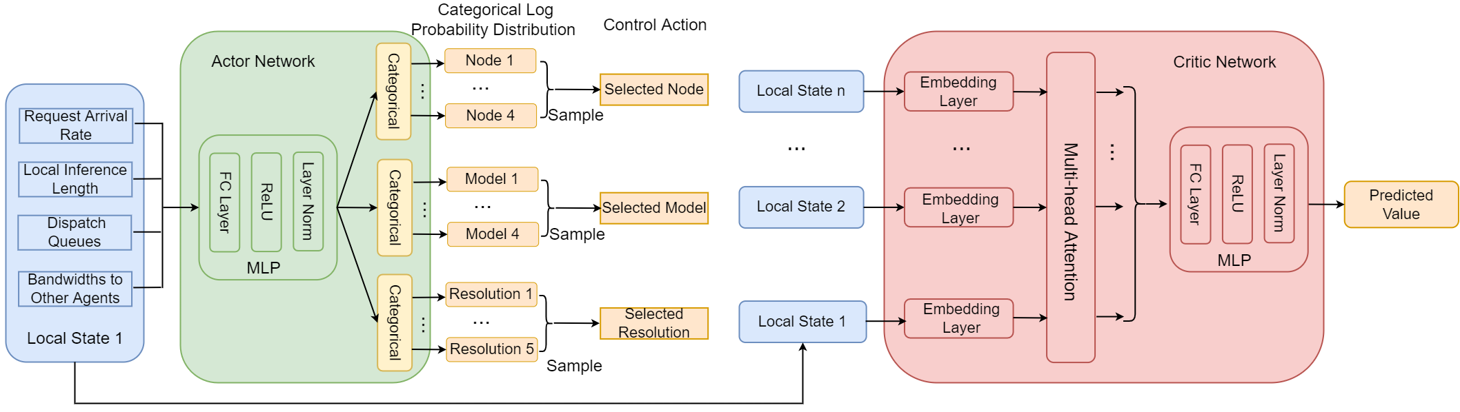
Figure 3: The network structure of the actor network and the critic network.

Design of actor network and critic network: The network structures of the actor network and the critic network are illustrated in Fig. 3. The inputs of the actor network are the local state of the edge node defined in Eq. (1), including the average inference request arrival rate during the past several time slots, the current length of the local inference queue, the current lengths of the dispatching queues to other edge nodes, and the bandwidths between an edge node and the other edge nodes. The average inference request arrival rate during the past several time slots on an edge node evaluates the edge node’s incoming workload, and the current length of the local inference queue describes the edge node’s pending workload. The current lengths of dispatching queues and the bandwidths between an edge node and other edge nodes evaluate the dispatching delay.

The outputs of the actor network are the categorical log probability distributions of three discrete actions. Our method can generate the discrete control actions by sampling from the categorical distributions. The control actions of an agent are defined in Eq. (3), including the selected edge node for inference, the selected DNN model for inference, and the selected resolution for video frame preprocessing. The inputs of the critic network are the global state of the video analytics system defined in Eq. (2), which consists of the local states of all agents and reflects the current system information of the video analytics system. The output of the critic network is the predicted value of the reward-to-go.

V-C Learning with Attention Mechanism

During the training with the actor-critic framework, each agent’s critic network needs to know the local state information of other agents through communication. As the number of the edge nodes increases, the input dimension of the critic network will become larger, and some irrelevant information may prevent the critic network from better predicting the reward-to-go, which in turn affects the actor network in learning the optimal policy. To avoid paying attention to all agents’ information indiscriminately, we adopt the multi-head attention mechanism [31] to distill valuable information. As illustrated in Fig. 3, after passing through the embedding layer, the local states of the agents will be fed into the multi-head attention network to extract more valuable system information so that the critic network can predict better.

Local state embedding: The embedding layer consists of one layer of Multi-Layer Perceptron (MLP) network. Each agent has a separate trainable embedding network for a critic network. We denote the embedding network of agent $i$ as $\Theta_{i}$,

$$e_{i}=\Theta_{i}(o_{i}),$$ (8)

where $o_{i}$ denotes the local state of agent $i$ and is the input of the embedding network, and $e_{i}$ denotes the output of the embedding network for agent $i$.

Attention network: The outputs of the embedding networks consist of multiple vectors, which will be sent into the multi-head attention network. The multi-head attention network can extract more valuable system information through training. With the attention mechanism, we can help the critic network predict the reward-to-go better and improve the system performance. We denote the multi-head attention network for an agent as $\Psi$,

$$(\psi_{1},\psi_{2},...,\psi_{n})=\Psi(e_{1},e_{2},...,e_{n}),$$ (9)

where $e_{1},e_{2},...,e_{n}$ are the outputs of the embedding layers, and $\psi_{1},\psi_{2},...,\psi_{n}$ are the outputs of the multi-head attention network. The attention network maps from a query and a set of key-value pairs to a weighted sum of values. Specifically, the query, key, and value of agent $i$ are computed by the following linear transformation,

$$q_{i}=e_{i}W^{q},k_{i}=e_{i}W^{k},v_{i}=e_{i}W^{v},$$ (10)

where $W^{q}$, $W^{k}$, and $W^{v}$ are the transformation matrices, and their parameters can be trained. All agents’ queries, keys and values are combined into $Q$, $K$, $V$ matrices respectively. Then, $Q$, $K$, and $V$ matrices will perform scaled dot-product attention calculation to get the output matrix,

$$Attention(Q,K,V)=softmax(\frac{QK^{T}}{\sqrt{d}})V,$$ (11)

where $d$ is the dimension of the vectors, and $\frac{1}{\sqrt{d}}$ is the scaling factor to avoid getting extremely small gradient values.

The multi-head attention network can calculate the mutual influences at different positions from different representation subspaces. Therefore, the agents map the $Q$, $K$, and $V$ matrices to different representation subspaces through linear transformations, and then we can obtain different aspects of mutual influences through the attention function,

$$head_{j}=Attention(Q_{j},K_{j},V_{j}),j\in J,$$ (12)

$$Q_{j}=QW_{j}^{q},K_{j}=KW_{j}^{k},V_{j}=VW_{j}^{v},$$

where $head_{j}$ denotes the output matrix of the $j$-th representation subspace, $Q_{j},K_{j},V_{j}$ represent the query, key, and value matrix under the $j$-th representation subspace respectively.

After the $J$ output matrices are concatenated, they are aggregated by a linear transformation,

$$MHA(Q,K,V)=Concat(head_{1},...,head_{J})W^{o},$$ (13)

where $MHA(Q,K,V)$ represents the final output matrix obtained by the multi-head attention mechanism, $Concat$ represents the concatenation operation, and $W^{o}$ is the transformation matrix.

Attentive critics: Each agent has its critic network. We denote the final two-layer MLP network of the critic network for an agent as $f$. We concatenate the outputs of the multi-head attention network and feed it into the final two-layer MLP network. Then, we can get the predicted value,

$$v=f(\psi_{1},\psi_{2},...,\psi_{n}),$$ (14)

where $v$ represents the predicted value for an agent and is the output of the overall critic network.

V-D Training Methodology

We now illustrate how to train the actor and critic networks for each agent with the proposed algorithm. The details of the training process are described in Algorithm 1.

At each time slot $t$, each agent $i$ observes its local state $o_{i}(t)$ from the video analytics system and obtains the global state $s(t)$ by communicating with other agents. The local state $o_{i}(t)$ will be input to the actor network $\mu_{i,\theta}$ to get the categorical log probability distribution of each action, and the actions $a_{i}(t)$ are sampled from the categorical distributions,

$$p_{i}(t)=\mu_{i,\theta}(o_{i}(t)),a_{i}(t)\sim p_{i}(t),$$ (15)

where $p_{i}(t)$ denotes the categorical log probability distributions of agent $i$ at time slot $t$. Then, the system will perform video analytics for the inference requests according to the control actions. Finally, at the end of time slot $t$, each agent will calculate its reward $r_{i}(t)$ during time slot $t$ according to Eq. (5), and we can calculate the shared reward $r(t)$ during time slot $t$ according to Eq. (6). Each agent $i$ obtains its new local state $o_{i}(t+1)$ and the global state $s(t+1)$ from the video analytics system at the beginning of time slot $t+1$. The local state, global state, action, shared reward, new local state, and new global state will be stored as a transition into the experience buffer as $(o_{i}(t),s(t),a_{i}(t),r(t),o_{i}(t+1),s(t+1))$.

After an episode, the estimated advantage is calculated with Generalized Advantage Estimation (GAE) [32] in the trajectory $\tau$, and the reward-to-go is calculated in the trajectory. Finally, batches are sampled from all transitions in this trajectory to train the networks. The actor networks are trained according to the policy objective defined in Eq. (16). The critic networks are trained according to the loss objective defined in Eq. (17). Then, we optimize the policy objective and loss objective by Adam [33] optimizer.

Each agent has multiple discrete actions, and the actor network will generate a categorical distribution for each action. Then, the control actions are sampled from the categorical distributions. We denote the actor network of an agent as $\mu_{\theta}$. For each agent, the actor network optimize the control policy to improve the reward, and the actor network is updated by maximizing the following objective,

$$L(\theta)=\frac{1}{B}\sum_{i=1}^{B}[min(\eta_{i,\theta}\hat{A}_{i},clip(\eta_{i,\theta},1-\epsilon,1+\epsilon)\hat{A}_{i})$$ (16)

$$+\sigma S(\mu_{\theta}(o_{i}))],$$

where $B$ is the batch size to sample from the buffer, $\eta_{i,\theta}=\frac{\mu_{\theta}(a_{i}\mid o_{i})}{\mu_{\theta_{old}}(a_{i}\mid o_{i})}$ represents the probability ratio with importance sampling, and this allows samples under parameters $\theta_{old}$ to be used to update parameters $\theta$, $\hat{A}_{i}$ is calculated by GAE, and this is used to evaluate the quality of the state-action pair ($\hat{A}_{i}>0$, relatively good; otherwise relatively poor), $\epsilon$ is the hyperparameter that controls the clipping strength, and this is used to prevent the new policy function from changing too much relative to the old policy function, $S$ is the policy entropy used to increase exploration, and $\sigma$ is the coefficient of the policy entropy.

We denote the critic network of an agent as $V_{\phi}$. For each agent, the goal of the critic network is to make the predicted value closer to the reward-to-go. The critic network is updated by minimizing the following loss,

$$C(\phi)=\frac{1}{B}\sum_{i=1}^{B}max[(V_{\phi}(s_{i})-\hat{R}_{i})^{2},(clip(V_{\phi}(s_{i}),$$ (17)

$$V_{\phi_{old}}(s_{i})-\varepsilon,V_{\phi_{old}}(s_{i})+\varepsilon)-\hat{R}_{i})^{2}],$$

where $\hat{R}_{i}$ is the reward-to-go, $s_{i}$ is the global state obtained from the buffer, $V_{\phi}$ is the value function (i.e., critic network) under parameters $\phi$, $V_{\phi_{old}}$ is the value function under parameters $\phi_{old}$, $\varepsilon$ is the hyperparameter that controls the clipping strength of the value loss to prevent the new value function from changing too much compared with the old value function.

Algorithm 1 Training Procedure

1:  Initialize the parameters $\theta$ of the actor $\mu$ and the parameters $\phi$ of the critic $V$

2:  Initialize the video analytics system

3:  Observe the agents’ local states $o_{1}(t),...,o_{n}(t)$ and the global state $s(t)$

4:  for $episode=1,...,M$ do

5:     $\tau_{1},...,\tau_{n}=[]$

6:     for $t=1,...,T$ do

7:        Get actions $a(t)=(a_{1}(t),...,a_{n}(t))$ by Eq. (15)

8:        Execute the joint actions $a(t)$

9:        Get the shared reward $r(t)$ by Eq. (6)

10:        Observe new state $s(t+1),o(t+1)$

11:        for each agent $i$ do

12:           $\tau_{i}+=[o_{i}(t),s(t),a_{i}(t),r(t),o_{i}(t+1),s(t+1)]$

13:        end for

14:     end for

15:     for each agent $i$ do

16:        Put $\tau_{i}$ into the replay buffer of agent $i$

17:        Compute advantage estimate $\hat{A}$ by GAE on $\tau_{i}$

18:        Compute reward-to-go $\hat{R}$ on $\tau_{i}$

19:        for num-mini-batch $j=1,...,J$ do

20:           $batch=$ randomly select mini-batch from the replay buffer of agent $i$

21:           Update $\theta$ on $L_{\theta}$ with data $batch$ via Adam

22:           Get predicted value for each transition by Eq. (14)

23:           Update $\phi$ on $C_{\phi}$ with data $batch$ via Adam

24:        end for

25:     end for

26:  end for

VI Performance Evaluation

In this section, we illustrate the experimental settings and evaluate the performance of our proposed method.

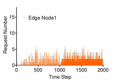
(a) Edge node 1.

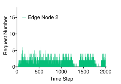
(b) Edge node 2.

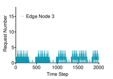
(c) Edge node 3.

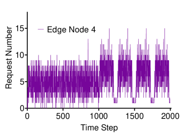
(d) Edge node 4.

Figure 4: The workload profiles of the four edge nodes.

VI-A Experimental Setting

Testbed: We consider a collaborative video analytics system with four edge nodes. Each edge node is equipped with an Inter(R) Xeon(R) Gold 6242R CPU and a GeForce RTX 2080Ti GPU. The operating system of the edge nodes is Ubuntu 18.04, and the video analytics system is built with Pytorch and Python. The test video contents are road traffic videos[34]. We use the publicly available bandwidth traces [35] to emulate the bandwidth connections between the edge nodes. Because there are no publicly available datasets for inference request rates, we simulate the arrival rates of inference requests on different edge nodes by scaling the request rates of the Wikipedia website [36]. The workload profiles of the edge nodes are shown in Fig. 4. The request rates on one edge node is light compared with its processing capacity. There are also two edge nodes with moderate request rates and one more edge node with a heavy workload.

System configuration: We consider the video analytics task of object detection for case study. We deploy four DNN-based object detection models on each edge node, including two small models (i.e., fasterrcnn mobilenet 320 and fasterrcnn mobilenet [37]) and two large models (i.e., retinanet resnet-50 [38] and maskrcnn resnet-50 [39]). The default penalty weight for the overall delay is set to be 5. The original video resolution is 1080P, which can be downsized to 720P, 480P, 360P, and 240P by video preprocessing. The recognition accuracy and the average inference delay for a video frame under different models and resolutions are illustrated in Table II and Table III, respectively. We calculate the recognition accuracy of a model under different video resolutions by comparing with the ground truth obtained from the recognition results of the most accurate model under the original resolution. This approach is consistent with the previous works [1, 25, 40].

TABLE II: The accuracy under different configurations.

Model name	1080P	720P	480P	360P	240P
fasterrcnn mobilenet 320	0.4158	0.4056	0.3834	0.3795	0.3426
fasterrcnn mobilenet	0.6503	0.6194	0.5987	0.5676	0.5055
retinanet resnet-50	0.8202	0.7630	0.7341	0.6917	0.5858
maskrcnn resnet-50	0.8614	0.8102	0.7807	0.7457	0.6191

TABLE III: The average delay under different configurations.

Model name	1080P	720P	480P	360P	240P
fasterrcnn mobilenet 320	0.087s	0.056s	0.037s	0.030s	0.026s
fasterrcnn mobilenet	0.103s	0.065s	0.044s	0.039s	0.034s
retinanet resnet-50	0.147s	0.113s	0.088s	0.074s	0.068s
maskrcnn resnet-50	0.171s	0.138s	0.110s	0.090s	0.074s

Training setup: The MARL algorithm is trained over 50,000 episodes, and each episode has 100 time steps. The duration of one time step is 0.2s. The MLP networks in both of the actor network and the critic network have two hidden layers, and each layer has 128 neurons. The activation function is ReLU, and LayerNorm is applied on each hidden layer. The outputs of the actor network consist of three categorical distributions corresponding to the three actions, and the output of the critic network is the predicted value. The embedding network consists of one layer with 8 neurons, and the number of outputs of the embedding network is 8. The multi-head attention network has 8 heads in the experiment. The learning rate is 0.0005. The entropy coefficient is $0.01$. The hyperparameter of clip is 0.2.

Baseline methods: We compare the performance of our method with the following baseline methods.

1) IPPO: the edge nodes learn their policies independently with Proximal Policy Optimization (PPO), which is a single-agent reinforcement learning method without communications among agents.

2) Local-PPO: each edge node only processes inference requests locally without dispatching them to other edge nodes, and selects models and resolutions with PPO.

3) Shortest-Queue: the arriving inference requests during a time slot will be forwarded to the edge node with the shortest waiting queue length. Meanwhile, we consider three methods to choose models and resolutions:

• Random: choose a random model and resolution.

• Min: choose the smallest model and the lowest resolution.

• Max: choose the largest model and highest resolution.

4) Random: the arriving inference requests on an edge node during a time slot will be randomly dispatched to an edge node. The model and resolution selection strategies include Random, Min, and Max.

5) Local: the arriving inference requests on an edge node will only be processed locally, combined with the model and resolution selection strategies of Random, Min, and Max.

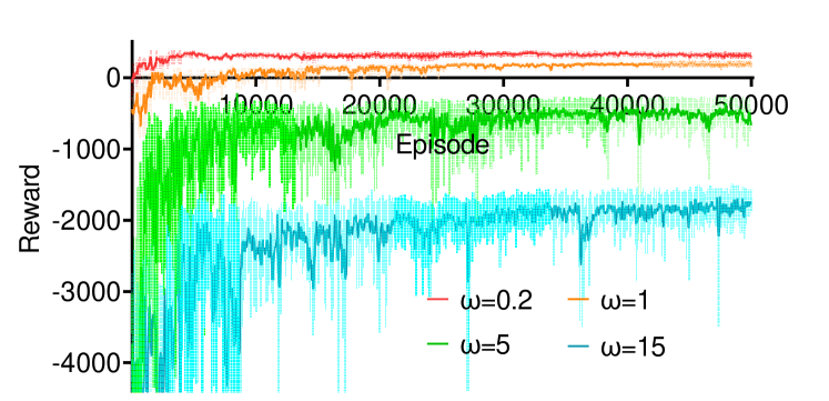
Figure 5: The convergence under different penalty weights.

VI-B Performance Analysis

We analyze the convergence and the performance characteristics of our method under different penalty weights (i.e., $\omega$) for the overall delay.

Convergence analysis: We first evaluate the convergence of the rewards of our method under different penalty weights ($\omega=0.2,1,5,15$) in Fig. 5. We can observe that the rewards of our method can converge and the optimal policies can be learned under different weights. The converged rewards are smaller under larger penalty weights for the overall delay. This is because it incurs a more penalty for the reward under the same delay with a larger weight.

Performance characteristic: We evaluate the performance characteristics of our method under different weights in Fig. 6 and 7, including the distributions of selected models and resolutions, average inference accuracy and overall delay per video frame, average request dispatching percentage, and average video frame drop percentage.

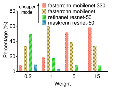
(a) Distributions of selected models.

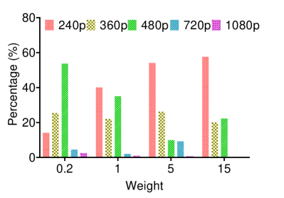
(b) Distribution of selected resolutions.

Figure 6: The distributions of selected DNN modes for inference and selected resolutions for preprocessing under different weights.

Fig. 6(a) illustrates the distribution of the selected DNN models for inference on the edge nodes under different weights. We can observe that the selected percentage of the large models becomes smaller (i.e., maskrcnn resnet-50 and retinanet resnet-50) as the weight increases. On the contrary, the selected percentage of the small model becomes larger (i.e., fasterrcnn mobilenet 320). This is because that choosing a cheaper model incurs smaller inference delay, thus leading to a higher reward under a larger penalty weight.

Fig. 6(b) illustrates the distribution of the selected video resolutions for preprocessing on the edge nodes under different weights. We can observe that the percentage of choosing a high resolution (i.e., 1080P) decreases as the weight increases. Conversely, the percentage of video frames being downsized to a lower resolution (i.e., 240P) gradually increases. This is because downsizing a video frame to a lower resolution will reduce inference and transmission delay, thus improving the reward when the delay is more important.

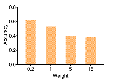
(a) Average inference accuracy.

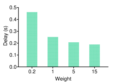
(b) Average overall delay.

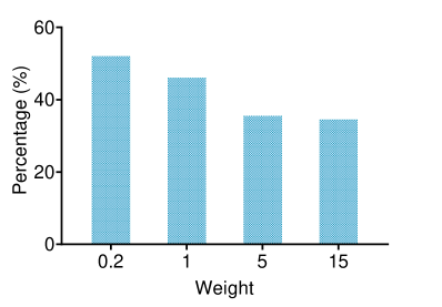
(c) Average dispatch percentage.

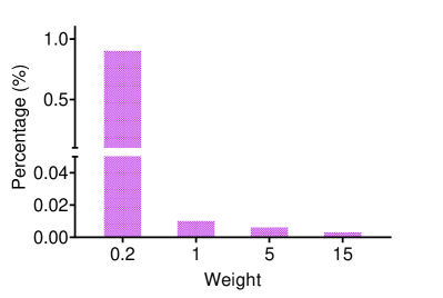
(d) Average drop percentage.

Figure 7: The average inference accuracy and overall delay per video frame, average request dispatching percentage, and video frame drop percentage under different weights.

Fig. 7(a) illustrates the average inference accuracy of the edge nodes under different weights. As the weight increases, the average inference accuracy decreases. This is because more video frames will be downsized to lower resolutions and analyzed with smaller models under a larger weight, leading to a decrease in the average inference accuracy.

Fig. 7(b) illustrates the average overall delay for a video frame under different weights. As the weight increases, the average overall delay for a video frame decreases. This is because with more video frames downsized to lower resolutions and analyzed with smaller models, the transmission and inference delay will decrease under larger weights.

Fig. 7(c) illustrates the average request dispatching percentage in the video analytics system under different weights. As the weight increases, the average dispatch percentage in the system decreases. This is because more video frames are analyzed locally to avoid transmission delay.

Fig 7(d) illustrates the average video frame drop percentage in the video analytics system under different weights. As the weight increases, the average video frame drop percentage in the system decreases. This is because smaller models and lower resolutions are selected for video analytics with larger weights, which can reduce inference delay and transmission delay to improve system processing capacity. Therefore, the video frame drop percentage will become lower.

VI-C Performance Comparison

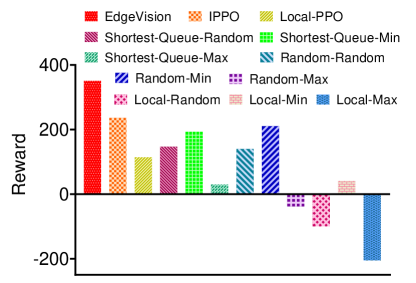
(a) $\omega=0.2$.

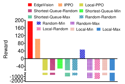
(b) $\omega=1$.

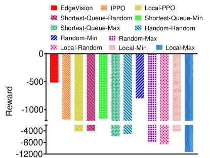
(c) $\omega=5$.

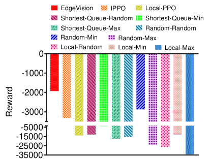
(d) $\omega=15$.

Figure 8: The comparison of the average rewards per episode of different methods under different weights.

We compare the average reward per episode of our method with the baseline methods under different weights in Fig. 8. We can observe in Fig. 8 that our method can achieve higher rewards compared with the baseline methods under different weights. IPPO achieves lower rewards and is more unstable during training compared with our method, because each agent learns its policy independently.

When the workload of an edge node is heavy, the baseline methods which only process video frames locally without dispatching (i.e., Locall-PPO, Local-Random, Local-Min, and Local-Max) have poor performance, because the edge nodes cannot cooperate with others to utilize the spare resources on others to process inference requests.

When the penalty weight is relatively large (i.e., $\omega=5,15$), the baseline methods that adopt the most complex model and the highest resolution (i.e., Shortest-Queue-Max, Random-Max, Local-Max) have poor performance due to the large inference delay and transmission delay. Choosing the cheapest model and lowest resolution (i.e., Shortest-Queue-Min and Random-Min) can reduce overall delay and increase rewards. However, the rewards are still lower than our method, because our method can dynamically choose the most appropriate resolution, model, and edge node for video frames.

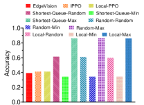
(a) Average inference accuracy.

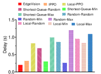
(b) Average overall delay.

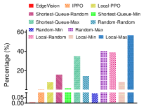
(c) Average drop percentage.

Figure 9: The comparison of the average accuracy, overall delay and video frame drop percentage of different methods under default weight.

We dissect the average rewards and illustrate the performance metrics of average accuracy, average overall delay, and average video frame drop percentage of different methods under the default penalty weight (i.e., $\omega=5$) in Fig. 9. The performance metrics under other weights also show similar observations. As shown in Fig. 9(a), our method has close accuracy to IPPO. However, our method can achieve a much lower overall delay and video frame drop percentage, as observed in Fig. 9(b) and Fig. 9(c). This verifies that our method can schedule the inference requests more efficiently among the edge nodes, thereby achieving higher performance.

The average accuracy of Local-PPO is close to our method. However, each edge node can only process inference requests independently without dispatching under Local-PPO. When the workload of an edge node is heavy, it will lead to long queuing delay, and more video frames will be dropped. Therefore, Local-PPO incurs larger overall delay and video frame drop percentage, as shown in Fig. 9(b) and Fig. 9(c). Local-Random, Local-Min, and Local-Max have similar problems. As shown in Fig. 9(b) and Fig. 9(c), these methods also incur large overall delay and frame drop percentages, resulting in poor performance.

The baseline methods of Shortest-Queue-Min and Random-Min always choose the cheapest model and the lowest resolution. We can observe in Fig. 9(a) and Fig. 9(b) that these methods have the lowest inference accuracy and the smallest overall delay. These methods have lower performance due to the fact that they cannot dynamically choose the most appropriate model and resolution. However, as shown in Fig. 9(c), the video frame drop percentages of these methods are higher compared with our method, and this is because these methods cannot schedule inference requests among edge nodes effectively, resulting in poor performance.

As the methods of Shortest-Queue-Max, Random-Max, and Local-Max always choose the largest model and the highest resolution, we can observe in Fig. 9(a) and Fig. 9(b) that these methods can achieve the highest accuracy but incur the largest overall delay. As shown in 9(c), these methods have high video frame drop percentages, which indicates that the system processing capacity is insufficient under these methods. These methods perform poorly under large penalty weights due to the large overall delay. Although the inference requests can be dispatched among different edge nodes with Shortest-Queue-Max and Random-Max, these methods still lead to large queuing delay and video frame drop percentages.

VI-D Ablation Study

We illustrate the ablation study of our method under different penalty weights in Fig. 10 to analyze the impact of the different components of our method. W/O Attention represents removing the attention network from our method, and W/O Other’s State represents removing the state information of other agents from the inputs of the critic network of an agent in our method.

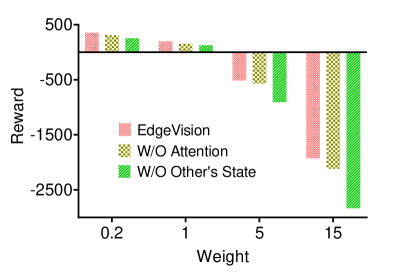
(a) Average reward.

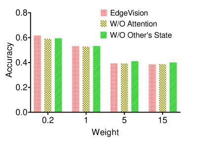
(b) Average accuracy.

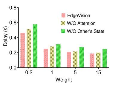
(c) Average overall delay.

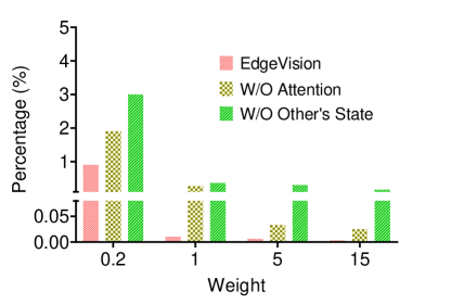
(d) Average drop percentage.

Figure 10: The ablation study under different penalty weights.

We illustrate the average reward per episode and the performance metrics of average accuracy, average overall delay, and average video frame drop percentage under different penalty weights in Fig. 10. As shown in Fig. 10(a), our method has the highest reward under different weights compared with W/O Attention and W/O other’s State. W/O Other’s State has the worst performance under different weights, which verifies that it is difficult for the agents to learn optimal policies only based on their local states. Therefore, the critic network of an agent needs the information of other edge nodes in the training process to learn the optimal policy. W/O Attention has lower performance compared with our method, because its critic networks pay undifferentiated attention to the information of all agents. Some useless and uninformative states will affect the training effect, resulting in lower performance. Our method can improve the rewards by 13.2%, 30.0%, 11.2%, and 10.1% compared with W/O Attention, and improve the rewards by 38.7%, 53.5%, 42.9%, and 32.8% compared with W/O Other’s State, under the weights of 0.2, 1, 5, and 15, respectively.

We can observe from Fig. 10(b) that our method has the highest accuracy when $\omega$ is 0.2, which indicates that our method chooses a more complex model and a higher resolution to handle inference requests. Furthermore, Fig. 10(c) and Fig. 10(d) show that our method has the lowest overall delay and video frame drop percentage, which verifies that it can schedule inference requests more efficiently and select more appropriate models and resolutions. When $\omega$ is 1 , Fig. 10(b) shows that the three methods have close accuracy, while Fig. 10(c) and Fig. 10(d) show that our method is better in terms of overall delay and video frame drop percentage. When $\omega$ is 5 and 15, Fig 10(b) shows that W/O Other’s State has higher accuracy, because this method chooses a more complex model and a higher resolution. However, Fig. 10(c) and Fig. 10(d) show that it has higher overall delay and video frame drop percentage, resulting in poor performance compared with our method.

VII Conclusion

In this paper, we propose an attention-driven MARL approach to learn the optimal policy for video analytics with multi-edge-node collaboration. We consider each edge node as an agent, which can cooperate with the other agents to jointly process the inference requests from different regions. The edge nodes can work fully cooperatively for video frame preprocessing, model selection, and request dispatching to minimize the overall system cost. We implement a video analytics testbed with multiple edge nodes and utilize real-world datasets to evaluate the performance of our method and to compare our performance with numerous baseline methods. The experimental results show that our proposed method can significantly improve the overall system performance and achieve a higher reward compared with the baseline methods.

References

- [1] Z. Xiao, Z. Xia, H. Zheng, B. Y. Zhao, and J. Jiang, “Towards performance clarity of edge video analytics,” in 2021 IEEE/ACM Symposium on Edge Computing (SEC). IEEE, 2021, pp. 148–164.
- [2] J. Jiang, Z. Luo, C. Hu, Z. He, Z. Wang, S. Xia, and C. Wu, “Joint model and data adaptation for cloud inference serving,” in 2021 IEEE Real-Time Systems Symposium (RTSS). IEEE, 2021, pp. 279–289.
- [3] X. Wang, G. Gao, X. Wu, Y. Lyu, and W. Wu, “Dynamic dnn model selection and inference off loading for video analytics with edge-cloud collaboration,” in Proceedings of the 32nd Workshop on Network and Operating Systems Support for Digital Audio and Video, 2022, pp. 64–70.
- [4] G. Ananthanarayanan, P. Bahl, P. Bodík, K. Chintalapudi, M. Philipose, L. Ravindranath, and S. Sinha, “Real-time video analytics: The killer app for edge computing,” computer, vol. 50, no. 10, pp. 58–67, 2017.
- [5] S. Yi, Z. Hao, Q. Zhang, Q. Zhang, W. Shi, and Q. Li, “Lavea: Latency-aware video analytics on edge computing platform,” in Proceedings of the Second ACM/IEEE Symposium on Edge Computing, 2017, pp. 1–13.
- [6] B. Qian, Z. Wen, J. Tang, Y. Yuan, A. Y. Zomaya, and R. Ranjan, “Osmoticgate: Adaptive edge-based real-time video analytics for the internet of things,” IEEE Transactions on Computers, 2022.
- [7] X. Wang and G. Gao, “Smarteye: An open source framework for real-time video analytics with edge-cloud collaboration,” in Proceedings of the 29th ACM International Conference on Multimedia, 2021, pp. 3767–3770.
- [8] X. Ran, H. Chen, X. Zhu, Z. Liu, and J. Chen, “Deepdecision: A mobile deep learning framework for edge video analytics,” in IEEE INFOCOM 2018-IEEE Conference on Computer Communications. IEEE, 2018, pp. 1421–1429.
- [9] T. Tan and G. Cao, “Deep learning video analytics through edge computing and neural processing units on mobile devices,” IEEE Transactions on Mobile Computing, 2021.
- [10] K. Zhao, Z. Zhou, X. Chen, R. Zhou, X. Zhang, S. Yu, and D. Wu, “Edgeadaptor: Online configuration adaption, model selection and resource provisioning for edge dnn inference serving at scale,” IEEE Transactions on Mobile Computing, 2022.
- [11] Y. Li, A. Padmanabhan, P. Zhao, Y. Wang, G. H. Xu, and R. Netravali, “Reducto: On-camera filtering for resource-efficient real-time video analytics,” in Proceedings of the Annual conference of the ACM Special Interest Group on Data Communication on the applications, technologies, architectures, and protocols for computer communication, 2020, pp. 359–376.
- [12] M. Li, Y. Li, Y. Tian, L. Jiang, and Q. Xu, “Appealnet: An efficient and highly-accurate edge/cloud collaborative architecture for dnn inference,” in 2021 58th ACM/IEEE Design Automation Conference (DAC). IEEE, 2021, pp. 409–414.
- [13] Y. Wang, W. Wang, J. Zhang, J. Jiang, and K. Chen, “Bridging the Edge-Cloud barrier for real-time advanced vision analytics,” in 11th USENIX Workshop on Hot Topics in Cloud Computing (HotCloud 19), 2019.
- [14] G. Ma, Z. Wang, M. Zhang, J. Ye, M. Chen, and W. Zhu, “Understanding performance of edge content caching for mobile video streaming,” IEEE Journal on Selected Areas in Communications, vol. 35, no. 5, pp. 1076–1089, 2017.
- [15] Y. Zhang, J.-H. Liu, C.-Y. Wang, and H.-Y. Wei, “Decomposable intelligence on cloud-edge iot framework for live video analytics,” IEEE Internet of Things Journal, vol. 7, no. 9, pp. 8860–8873, 2020.
- [16] A. H. Jiang, D. L.-K. Wong, C. Canel, L. Tang, I. Misra, M. Kaminsky, M. A. Kozuch, P. Pillai, D. G. Andersen, and G. R. Ganger, “Mainstream: Dynamic Stem-Sharing for Multi-Tenant video processing,” in 2018 USENIX Annual Technical Conference (USENIX ATC 18), 2018, pp. 29–42.
- [17] M. Zhang, F. Wang, Y. Zhu, J. Liu, and Z. Wang, “Towards cloud-edge collaborative online video analytics with fine-grained serverless pipelines,” in Proceedings of the 12th ACM Multimedia Systems Conference, 2021, pp. 80–93.
- [18] Y. Huang, F. Wang, F. Wang, and J. Liu, “Deepar: A hybrid device-edge-cloud execution framework for mobile deep learning applications,” in IEEE INFOCOM 2019-IEEE Conference on Computer Communications Workshops (INFOCOM WKSHPS). IEEE, 2019, pp. 892–897.
- [19] C. Long, Y. Cao, T. Jiang, and Q. Zhang, “Edge computing framework for cooperative video processing in multimedia iot systems,” IEEE Transactions on Multimedia, vol. 20, no. 5, pp. 1126–1139, 2017.
- [20] Z. Fu, J. Ren, D. Zhang, Y. Zhou, and Y. Zhang, “Kalmia: A heterogeneous qos-aware scheduling framework for dnn tasks on edge servers,” in IEEE INFOCOM 2022-IEEE Conference on Computer Communications. IEEE, 2022, pp. 780–789.
- [21] K. Du, A. Pervaiz, X. Yuan, A. Chowdhery, Q. Zhang, H. Hoffmann, and J. Jiang, “Server-driven video streaming for deep learning inference,” in Proceedings of the Annual conference of the ACM Special Interest Group on Data Communication on the applications, technologies, architectures, and protocols for computer communication, 2020, pp. 557–570.
- [22] C. Pakha, A. Chowdhery, and J. Jiang, “Reinventing video streaming for distributed vision analytics,” in 10th USENIX workshop on hot topics in cloud computing (HotCloud 18), 2018.
- [23] T. Elgamal, S. Shi, V. Gupta, R. Jana, and K. Nahrstedt, “Sieve: Semantically encoded video analytics on edge and cloud,” in 2020 IEEE 40th International Conference on Distributed Computing Systems (ICDCS). IEEE, 2020, pp. 1383–1388.
- [24] C. Canel, T. Kim, G. Zhou, C. Li, H. Lim, D. G. Andersen, M. Kaminsky, and S. Dulloor, “Scaling video analytics on constrained edge nodes,” Proceedings of Machine Learning and Systems, vol. 1, pp. 406–417, 2019.
- [25] J. Jiang, G. Ananthanarayanan, P. Bodik, S. Sen, and I. Stoica, “Chameleon: scalable adaptation of video analytics,” in Proceedings of the 2018 Conference of the ACM Special Interest Group on Data Communication, 2018, pp. 253–266.
- [26] C. Wang, S. Zhang, Y. Chen, Z. Qian, J. Wu, and M. Xiao, “Joint configuration adaptation and bandwidth allocation for edge-based real-time video analytics,” in IEEE INFOCOM 2020-IEEE Conference on Computer Communications. IEEE, 2020, pp. 257–266.
- [27] H. Zhang, G. Ananthanarayanan, P. Bodik, M. Philipose, P. Bahl, and M. J. Freedman, “Live video analytics at scale with approximation and Delay-Tolerance,” in 14th USENIX Symposium on Networked Systems Design and Implementation (NSDI 17), 2017, pp. 377–392.
- [28] C.-C. Hung, G. Ananthanarayanan, P. Bodik, L. Golubchik, M. Yu, P. Bahl, and M. Philipose, “Videoedge: Processing camera streams using hierarchical clusters,” in 2018 IEEE/ACM Symposium on Edge Computing (SEC). IEEE, 2018, pp. 115–131.
- [29] X. Zeng, B. Fang, H. Shen, and M. Zhang, “Distream: scaling live video analytics with workload-adaptive distributed edge intelligence,” in Proceedings of the 18th Conference on Embedded Networked Sensor Systems, 2020, pp. 409–421.
- [30] D. S. Bernstein, R. Givan, N. Immerman, and S. Zilberstein, “The complexity of decentralized control of markov decision processes,” Mathematics of operations research, vol. 27, no. 4, pp. 819–840, 2002.
- [31] A. Vaswani, N. Shazeer, N. Parmar, J. Uszkoreit, L. Jones, A. N. Gomez, Ł. Kaiser, and I. Polosukhin, “Attention is all you need,” Advances in neural information processing systems, vol. 30, 2017.
- [32] J. Schulman, P. Moritz, S. Levine, M. Jordan, and P. Abbeel, “High-dimensional continuous control using generalized advantage estimation,” arXiv preprint arXiv:1506.02438, 2015.
- [33] D. P. Kingma and J. Ba, “Adam: A method for stochastic optimization,” arXiv preprint arXiv:1412.6980, 2014.
- [34] J. Utah, “Traffic camera videos and dash camera videos,” Mar 2018, https://www.youtube.com/channel/UCBcVQr-07MH-p9e2kRTdB3A/videos.
- [35] Z. Akhtar, Y. S. Nam, R. Govindan, S. Rao, J. Chen, E. Katz-Bassett, B. Ribeiro, J. Zhan, and H. Zhang, “Oboe: Auto-tuning video abr algorithms to network conditions,” in Proceedings of the 2018 Conference of the ACM Special Interest Group on Data Communication, 2018, pp. 44–58.
- [36] G. Urdaneta, G. Pierre, and M. Van Steen, “Wikipedia workload analysis for decentralized hosting,” Computer Networks, vol. 53, no. 11, pp. 1830–1845, 2009.
- [37] S. Ren, K. He, R. Girshick, and J. Sun, “Faster r-cnn: Towards real-time object detection with region proposal networks,” Advances in neural information processing systems, vol. 28, 2015.
- [38] T.-Y. Lin, P. Goyal, R. Girshick, K. He, and P. Dollár, “Focal loss for dense object detection,” in Proceedings of the IEEE international conference on computer vision, 2017, pp. 2980–2988.
- [39] K. He, G. Gkioxari, P. Dollár, and R. Girshick, “Mask r-cnn,” in Proceedings of the IEEE international conference on computer vision, 2017, pp. 2961–2969.
- [40] D. Kang, J. Emmons, F. Abuzaid, P. Bailis, and M. Zaharia, “Noscope: optimizing neural network queries over video at scale,” arXiv preprint arXiv:1703.02529, 2017.