Improved torque estimator for condensed-phase quasicentroid molecular dynamics

Abstract

We describe improvements to the quasicentroid molecular dynamics (QCMD) path-integral method, which was developed recently for computing the infrared spectra of condensed-phase systems. The main development is an improved estimator for the intermolecular torque on the quasicentroid. When applied to qTIP4P/F liquid water and ice, the new estimator is found to remove an artificial $25$ cm^-1 red shift from the libration bands, to increase slightly the intensity of the OH stretch band in the liquid, and to reduce small errors noted previously in the QCMD radial distribution functions. We also modify the mass-scaling used in the adiabatic QCMD algorithm, which allows the molecular dynamics timestep to be quadrupled, thus reducing the expense of a QCMD calculation to twice that of Cartesian centroid molecular dynamics for qTIP4P/F liquid water at 300 K, and eight times for ice at 150 K.

I Introduction

Quasicentroid molecular dynamics (QCMD) is a recently developed path-integral dynamics method[1] which has given promising results for simulations of infrared spectra in gas and condensed phases.[1, 2, 3, 4] It avoids most of the well-characterised drawbacks[5, 6, 7, 8, 9, 10] of the related centroid molecular dynamics (CMD)[11, 12, 13] and (thermostatted) ring-polymer molecular dynamics [(T)RPMD][8, 10, 14, 15, 16] methods, by propagating classical trajectories on the potential of mean force (PMF) obtained by constraining a set of curvilinear centroids. These coordinates are system-dependent and chosen to give compact ring-polymer distributions in which the curvilinear centroid lies close to the Cartesian centroid and is hence referred to as the ‘quasicentroid’. As originally developed, QCMD uses a modification[1] of the adiabatic CMD propagator[12, 13] which makes QCMD more expensive than CMD (e.g., by a factor of 32 for qTIP4P/F[17] ice at 150 K), and thus much more expensive than (T)RPMD. However, exciting recent progress has been made in developing a fast QCMD (f-QCMD) algorithm,[4] which extracts a highly accurate approximation to the quasicentroid PMF from a static path-integral calculation.

In the gas-phase, QCMD has now been applied to water, ammonia and methane (the latter using f-QCMD).[1, 2, 3, 4] The positions and intensities of the fundamental bands are in excellent agreement with the exact quantum results, and the positions of the overtone and combination bands are in reasonable agreement. However, the intensities of the latter are an order of magnitude too small, which was shown recently[19, 20] to be because QCMD neglects coupling between the Matsubara dynamics[21, 22, 9, 23, 24] of the centroid and the fluctuation modes [as also do CMD, RPMD and classical molecular dynamics (MD)].[25]

In the condensed phase, QCMD has been tested on the qTIP4P/F water model, for the liquid at 300 K and for ice I${}_{\text{h}}$ at 150 K.[1, 2] Detailed comparisons with experiment are not possible for such a simple potential, but the QCMD results are promising: the spectra appear to inherit the advantages of the gas-phase QCMD calculations, with the stretch bands showing none of the artefacts that appear in the corresponding CMD and (T)RPMD spectra at low temperatures[27] and lining up well with the results of other simulation methods.[28, 29]

However, QCMD does appear to have introduced a minor artefact of its own into the qTIP4P/F spectra, in the form of a 25 cm^-1 red shift in the libration bands of both the liquid and ice.[1, 2] This is a numerically small error, but it might become larger in other condensed-phase calculations, because it is most likely caused by errors in the estimator for the intermolecular torque $\overline{\bm{\tau}}$ (between the quasicentroids of pairs of monomers). Unlike the other components of the PMF, $\overline{\bm{\tau}}$ needed to be approximated in order to make the simulations practical, and the ad hoc assumption was made[1] that $\overline{\bm{\tau}}$ could be approximated as the average of the torques on the individual ring-polymer beads.

Here, we introduce a new estimator for $\overline{\bm{\tau}}$ and report numerical tests which show that it removes the 25 cm^-1 red-shift from the qTIP4P/F libration bands, increases slightly the intensity of the stretch band in the liquid, and reduces small errors in the radial distribution functions (noted in previous QCMD calculations at 300 K[1]). After summarising the theory of QCMD in Sec. II, we introduce the new $\overline{\bm{\tau}}$ estimator in Sec. III, and report the tests on qTIP4P/F water in Sec. IV. We also (Sec. IV.1) introduce a straightforward modification to the adiabatic QCMD propagator which improves numerical stability and speeds up the calculation by a factor of four. Section V concludes the article.

II Background theory

In QCMD, the dynamics are approximated by classical trajectories on a quantum potential of mean force, which is obtained by sampling the quantum Boltzmann distribution as a function of a set of curvilinear centroid coordinates. The usual Cartesian ‘ring-polymers’ [30, 31] are used to represent the distribution.

For a gas-phase system, the distribution takes the form ${\cal{N}}^{-1}\exp[-\beta W({\bf q})]$, in which ${\cal{N}}$ is a normalisation factor, $\beta=1/k_{\mathrm{B}}T$, and

$$W(\mathbf{q})=U(\mathbf{q})+S(\mathbf{q}),$$ (1a)

$$U(\mathbf{q})=\frac{1}{N}\sum_{i=1}^{N}V(\mathbf{q}_{i}),$$ (1b)

$$S(\mathbf{q})=\frac{N}{2(\beta\hbar)^{2}}\sum_{\alpha=1}^{n}\sum_{i=1}^{N}m_{\alpha}\big{\lVert}\mathbf{q}^{(\alpha)}_{i+1}-\mathbf{q}^{(\alpha)}_{i}\big{\rVert}^{2},$$ (1c)

where $V$ is the system potential, $n$ is the number of atoms, $m_{\alpha}$ is the mass of atom $\alpha$, $\mathbf{q}^{(\alpha)}_{\mkern 3.0mui}\!\equiv\big{(}q^{(\alpha)}_{1,i},\,q^{(\alpha)}_{2,i},\,q^{(\alpha)}_{3,i}\big{)}$, and $q_{\mathrlap{\mkern 2.0mu\rule{0.0pt}{4.52083pt}\nu}}{}^{(\alpha)}$ are a set of $N$ replica ‘beads’ of the Cartesian coordinates ($\nu$=1,2,3 corresponding to $x,y,z$) of atom $\alpha$.

The curvilinear centroid coordinates are system-dependent and are chosen to make the distribution compact, such that the molecular geometry specified by the curvilinear centroids, called the ‘quasicentroid’, is close to the geometry specified by the (Cartesian) centroids of the atoms (i.e., the centres of mass of $\mathbf{q}^{(\alpha)}_{\mkern 3.0mui}$). For example, a good set of curvilinear centroids for gas-phase water are the bond-angle centroids

$$R_{1,2} =\frac{1}{N}\sum_{i}r_{i1,2},$$ (2)

$$\Theta =\frac{1}{N}\sum_{i}\theta_{i},$$

where $(r_{i1},r_{i2},\theta_{i})$ are the bond-angle coordinates of the individual beads. To generate the dynamics, the quasicentroid coordinates are converted to a set of cartesians, denoted ${\overline{\mathbf{Q}}}^{(\alpha)}$. One then propagates ${\overline{\mathbf{Q}}}^{(\alpha)}$ and the conjugate momenta ${\overline{\mathbf{P}}}^{(\alpha)}$ using standard Cartesian classical dynamics, with the forces generated by the PMF

$${-\frac{\partial{\overline{F}}}{\partial{\overline{\mathbf{Q}}^{(\alpha)}}}}\simeq{-\left\langle\frac{\partial{U}}{\partial{\overline{\mathbf{Q}}^{(\alpha)}}}\right\rangle,}$$ (3)

where $\langle\ldots\rangle$ denotes a quasicentroid-constrained average over the ring-polymer distribution. The trajectories are thermostatted, which ensures that they sample a good approximation to the exact quantum Boltzmann distribution, provided the quasicentroid-constrained distributions are sufficiently compact (which should always be checked numerically by comparing static thermal averages computed using QCMD and standard path-integral methods).

For a condensed-phase system, the ring-polymer distribution of Eq. (1) generalises in the usual way, to include a sum over all the molecules in the simulation cell, together with intermolecular components of the physical potential $V$ (including the usual Ewald-sum terms[33] to handle the periodic boundary conditions). In addition to internal components of the quasicentroid (e.g., Eq. (2) in the case of water), one must also define external components, to specify the centres of mass and orientations of the molecules. This is done by applying to the quasicentroids of each molecule the ‘Eckart-like’ conditions,[34, 35]

$$\sum_{\alpha}m_{\alpha}(\mathbf{Q}^{(\alpha)}-\overline{\mathbf{Q}}^{(\alpha)}) =\mathbf{0},$$ (4a)

$$\sum_{\alpha}m_{\alpha}\overline{\mathbf{Q}}^{(\alpha)}\!\times(\mathbf{Q}^{(\alpha)}-\overline{\mathbf{Q}}^{(\alpha)}) =\mathbf{0},$$ (4b)

where the sum is over the atoms in the molecule, and

$$\mathbf{Q}^{(\alpha)}=\frac{1}{N}\sum_{i=1}^{N}\mathbf{q}^{(\alpha)}_{i}$$ (5)

are the Cartesian centroids of atom $\alpha$. Equation (4a) constrains the quasicentroid centre of mass

$$\overline{\mathbf{Q}}_{\mathrm{com}}\equiv\frac{\sum_{\alpha}m_{\alpha}\overline{\mathbf{Q}}^{(\alpha)}}{\sum_{\alpha}m_{\alpha}}$$ (6)

to lie at the centroid centre of mass (i.e., the overall centre of mass of all the atomic bead coordinates in the molecule). Equation (4b) orients the atomic quasicentroids so as to minimise the mass-weighted sum of their square distances from the atomic quasicentroids ${\overline{\mathbf{Q}}}^{(\alpha)}$ (see Fig. 6 of Ref. 1). The potential gradient in the PMF then takes the form

$${-\frac{\partial{U}}{\partial{\overline{\mathbf{Q}}{}^{\mathrlap{(\alpha)}\ }}}\mkern 8.0mu}=\overline{\mathbf{f}}_{\mathrm{int}}+\overline{\mathbf{f}}_{\mathrm{trans}}+\overline{\mathbf{f}}_{\mathrm{rot}},$$ (7)

where $\overline{\mathbf{f}}_{\mathrm{int}}$ denotes the forces acting on the internal components of the centroid (e.g., $R_{1,2},\Theta$ in the case of water), $\overline{\mathbf{f}}_{\mathrm{trans}}$ denotes the forces between the monomer centres of mass, and $\overline{\mathbf{f}}_{\mathrm{rot}}$ the torques between pairs of monomers.

In Ref. 1, it is shown that $\overline{\mathbf{f}}_{\mathrm{int}}$ and $\overline{\mathbf{f}}_{\mathrm{trans}}$ can be evaluated directly, but that $\overline{\mathbf{f}}_{\mathrm{rot}}$ must be approximated. This is because $\overline{\mathbf{f}}_{\mathrm{rot}}$ is given by

$$\overline{\mathbf{f}}_{\mathrm{rot}}^{(\alpha)}\equiv m_{\alpha}(\mathbf{I}^{-1}\overline{\bm{\tau}})\times\overline{\mathbf{Q}}^{(\alpha)},$$ (8)

in which $\mathbf{I}$, the inertia tensor with elements

$$I_{\mu\nu}=\sum_{\alpha}m_{\alpha}\!\left[\Big{\lVert}\overline{\mathbf{Q}}{}^{(\alpha)}\Big{\rVert}^{\!2}\delta_{\mu\nu}-\overline{Q}^{(\alpha)}_{\mu}\overline{Q}^{(\alpha)}_{\nu}\right]\!,$$ (9)

can be be evaluated directly, but the quasicentroid torque,

$$\overline{\bm{\tau}}=-\sum_{\alpha}\left(\overline{\mathbf{Q}}{}^{(\alpha)}-\overline{\mathbf{Q}}_{\mathrm{com}}\right)\times\frac{\partial{U{\phantom{{}^{(\alpha)}}}}}{\partial{\overline{\mathbf{Q}}{}^{(\alpha)}}},$$ (10)

cannot be, because it depends on all the components of ${\partial U}/\partial{\overline{\mathbf{Q}}{}^{(\alpha)}}$. Reference 1 therefore introduced the ad hoc approximation

$$\overline{\bm{\tau}}\simeq\frac{1}{N}\sum_{i}{\bm{\tau}}_{i}$$ (11)

where ${\bm{\tau}}_{i}$ are the individual torques on the polymer beads. As mentioned in the Introduction, this approximation works well on the whole but is thought to be responsible for the 25 cm^-1 red shifts in the libration bands of the spectra of qTIP4P/F water and ice, as well as for small but noticeable discrepancies between the QCMD and PIMD radial distribution functions (RDFs).

III Improved torque estimator

We now propose a new estimator for $\overline{\bm{\tau}}$ which is based on a heuristic approximation to the following (exact) linear equations for $\mathbf{I}^{-1}\overline{\bm{\tau}}$,

$$\sum_{\alpha,\nu}m_{\alpha}\Big{\{}\overline{Q}{}_{\mu}^{(\alpha)}Q{}_{\nu}^{(\alpha)}-\big{(}\overline{\mathbf{Q}}{}^{(\alpha)}\!\cdot\mathbf{Q}{}^{(\alpha)}\big{)}\delta_{\mu\nu}\Big{\}}\Big{\{}\mathbf{I}^{-1}\overline{\bm{\tau}}\Big{\}}_{\nu}$$

$$\qquad{}=\sum_{\alpha}\left\{{-\frac{\partial{U}}{\partial{\overline{\mathbf{Q}}^{\mathrlap{(\alpha)}\ }}}\mkern 8.0mu}\times\mathbf{Q}{}^{(\alpha)}-\overline{\mathbf{f}}_{\mathrm{int}}\times\mathbf{Q}{}^{(\alpha)}\right\}_{\!\mu}$$ (12)

obtained by applying $\times\mathbf{Q}{}^{(\alpha)}$ to both sides of Eq. (7). These equations contain the difficult-to-evaluate derivatives ${\partial U}/\partial{\overline{\mathbf{Q}}{}^{(\alpha)}}$, but now crossed with the Cartesian centroid. In what follows, we give a heuristic justification for replacing this term by its easy-to-evaluate ‘complement’ ${\partial U}/\partial{\mathbf{Q}^{(\alpha)}}\times\overline{\mathbf{Q}}{}^{(\alpha)}$, giving

$$\sum_{\alpha,\nu}m_{\alpha}\Big{\{}\overline{Q}{}_{\mu}^{(\alpha)}Q{}_{\nu}^{(\alpha)}-\big{(}\overline{\mathbf{Q}}{}^{(\alpha)}\!\cdot\mathbf{Q}{}^{(\alpha)}\big{)}\delta_{\mu\nu}\Big{\}}\Big{\{}\mathbf{I}^{-1}\overline{\bm{\tau}}\Big{\}}_{\nu}$$

$$\qquad{}\simeq\sum_{\alpha}\left\{{-\frac{\partial{U}}{\partial{\mathbf{Q}^{\mathrlap{(\alpha)}\ }}}\mkern 8.0mu}\times\overline{\mathbf{Q}}{}^{(\alpha)}-\overline{\mathbf{f}}_{\mathrm{int}}\times\mathbf{Q}{}^{(\alpha)}\right\}_{\!\mu}.$$ (13)

These equations are cheap numerically to set up and solve at every timestep of the propagation, yielding $\mathbf{I}^{-1}\overline{\bm{\tau}}$ and thus $\overline{\mathbf{f}}_{\mathrm{rot}}$.

We justify this approximation by noting that the quasicentroid-constrained distributions are expected to be compact, such that $\overline{\mathbf{Q}}{}^{(\alpha)}$ is close to $\mathbf{Q}^{(\alpha)}$, and that the QCMD dynamics is expected to give a good approximation to the Matsubara dynamics of the centroids. All the normal modes of the ring-polymers evolve explicitly in time in Matsubara dynamics, which allows us to write out the second time-derivative of Eq. (4b) in the form

$$\sum_{\alpha}m_{\alpha}\ddot{\overline{\mathbf{Q}}}{}^{(\alpha)}\times\mathbf{Q}^{(\alpha)} ={}$$ (14)

$$\sum_{\alpha}m_{\alpha}\ddot{\mathbf{Q}}^{(\alpha)}\times\overline{\mathbf{Q}}{}^{(\alpha)} +2\sum_{\alpha}m_{\alpha}\dot{\mathbf{Q}}^{(\alpha)}\times\dot{\overline{\mathbf{Q}}}{}^{(\alpha)},$$

then to average over the quasicentroid-constrained quantum Boltzmann distribution, to obtain

$$\sum_{\alpha}\left\langle m_{\alpha}\ddot{\overline{\mathbf{Q}}}{}^{(\alpha)}\times\mathbf{Q}^{(\alpha)}\right\rangle= \sum_{\alpha}\left\langle m_{\alpha}\ddot{\mathbf{Q}}^{(\alpha)}\times\overline{\mathbf{Q}}{}^{(\alpha)}\right\rangle.$$ (15)

The final term in Eq. (14) has vanished under thermal averaging, since the component of the Cartesian centroid momentum $m_{\alpha}\dot{\mathbf{Q}}^{(\alpha)}$ that is orthogonal to $\dot{\overline{\mathbf{Q}}}{}^{(\alpha)}$ is isotropically distributed. Noting that forces in Matsubara dynamics are simply the negative derivatives of $U$ (and assuming that the quasicentroid curvature is sufficiently small that $m_{\alpha}\ddot{\overline{\mathbf{Q}}}{}^{(\alpha)}\simeq\dot{\overline{\mathbf{P}}}{}^{(\alpha)}$), we can then write

$$\sum_{\alpha}\left\langle{-\frac{\partial{U}}{\partial{\overline{\mathbf{Q}}{}^{\mathrlap{(\alpha)}\ }}}\mkern 8.0mu}\times\mathbf{Q}^{(\alpha)}\right\rangle\simeq \sum_{\alpha}\left\langle{-\frac{\partial{U}}{\partial{\mathbf{Q}^{\mathrlap{(\alpha)}\ }}}\mkern 8.0mu}\times\overline{\mathbf{Q}}{}^{(\alpha)}\right\rangle.$$ (16)

Finally, we note that the PMF requires only the quasi-centroid-constrained average $\left\langle\mathbf{I}^{-1}\overline{\bm{\tau}}\right\rangle$, and that Eq. (III) implies that

$$\sum_{\alpha,\nu}\left\langle m_{\alpha}\Big{\{}\overline{Q}{}_{\mu}^{(\alpha)}Q{}_{\nu}^{(\alpha)}-\big{(}\overline{\mathbf{Q}}{}^{(\alpha)}\!\cdot\mathbf{Q}{}^{(\alpha)}\big{)}\delta_{\mu\nu}\Big{\}}\right\rangle\left\langle\Big{\{}\mathbf{I}^{-1}\overline{\bm{\tau}}\Big{\}}_{\nu}\right\rangle$$

$$\qquad{}\simeq\sum_{\alpha}\left\langle\left\{{-\frac{\partial{U}}{\partial{\overline{\mathbf{Q}}^{\mathrlap{(\alpha)}\ }}}\mkern 8.0mu}\times\mathbf{Q}{}^{(\alpha)}-\overline{\mathbf{f}}_{\mathrm{int}}\times\mathbf{Q}{}^{(\alpha)}\right\}_{\!\mu}\right\rangle,$$ (17)

since the variance of $\mathbf{Q}^{(\alpha)}$ around $\overline{\mathbf{Q}}{}^{(\alpha)}$ is expected to be small. Combining Eqs. (16) and (III) leads to Eq. (III), which we now see should be a reasonable estimator for the quasicentroid torque, provided the quasicentroid-constrained distribution remains compact.

IV Tests for liquid water and ice

To test the new $\mathbf{I}^{-1}\overline{\bm{\tau}}$ estimator, we recalculated the qTIP4P/F infrared spectra of liquid water (300 K) and ice I${}_{\text{h}}$ (150 K) using the adiabatic QCMD (AQCMD) algorithm of Ref. 1. We also took the opportunity to improve the efficiency and stability of the algorithm, by modifying the mass scaling.

IV.1 Modified mass scaling

The AQCMD algorithm is a modification of the ACMD algorithm.[12, 13] The latter samples the (Cartesian) centroid-constrained ring-polymer distribution adiabatically, on the fly, by scaling the masses of the ring-polymer normal modes orthogonal to the centroid (to increase their vibrational frequencies) and thermostatting them aggressively. AQCMD applies the analogous procedure to generate the PMF of the quasicentroid on the fly. It achieves this by mass-scaling all ring-polymer degrees of freedom (including the Cartesian centroids) and by applying quasicentroid constraints to the thermostatted ring-polymer dynamics. The resulting AQCMD algorithm resembles the dynamics of two different systems (the ring-polymer beads and the quasicentroids) evolving in parallel.

The original version of ACMD scaled the masses $m$ associated with the ring-polymer normal modes orthogonal to the centroid ($n=\pm 1,\ldots,\pm\tfrac{N-2}{2},\tfrac{N}{2})$ to

$$m_{n}=\frac{m}{\kappa_{n}^{2}},\quad\kappa_{n}=\gamma\frac{\omega_{N}}{\omega_{n}},$$ (18)

where $\omega_{n}=2\omega_{N}\sin(\pi|n|/N)$ is the ring-polymer-spring frequency of mode $n$, $\omega_{N}\equiv N/\beta\hbar$, and $\gamma$ is the adiabaticity parameter. The limit $\gamma\to\infty$ corresponds to complete adiabatic separation between the dynamics of the centroid and the non-centroid modes, but in practice $\gamma=10$–$100$ is usually sufficient numerically. One aims to keep $\gamma$ as small as possible in order to use the largest possible timestep. The version of AQCMD of Ref. 1 used the scaling in Eq. (18) for the $n\neq 0$ modes, and additionally scaled the centroid ($n=0$) mass by $\kappa_{0}=\gamma$.

The problem with this choice of scaling (for both ACMD and AQCMD) is that it does not scale the frequencies of different normal modes evenly. For a harmonic component of $V$ of frequency $\Omega$, the resulting scaled frequencies are

$$\widetilde{\Omega}_{n}=\kappa_{n}\sqrt{\omega_{n}^{2}+\Omega^{2}}.$$ (19)

(where the $\omega_{n}^{2}$ originates from the spring potential $S$). Figure 1 shows that ${\Omega}_{n}$ has a flat distribution for $\Omega=500$ cm^-1 (roughly the libration frequency of water), but that it has a spike at low $n$ for $\Omega=3500$ cm^-1 (roughly the OH stretch fequency). As a result, $\widetilde{\Omega}_{n}$ becomes larger than numerically necessary for low $n$, resulting in the need for a particularly small timestep. Also, in AQCMD the (arbitrarily chosen) $\kappa_{0}=\gamma$ scaling of the centroid shifts the frequency of this mode significantly less than that of the other modes.

We thus use a new mass-scaling similar to that employed in the i-PI package[40] implementation of ACMD. We take

$$\kappa_{n}=\frac{\gamma\omega_{N}}{\sqrt{\omega_{n}^{2}+\Omega_{\text{ref}}^{2}}}.$$ (20)

for all $n$ (including $n=0$). Setting the ‘reference frequency’ $\Omega_{\text{ref}}=2500~{}\mathrm{cm}^{-1}$, we obtain the revised $\widetilde{\Omega}_{n}$ distribution shown in Fig. 1 (black crosses). Clearly the revised $\widetilde{\Omega}_{n}$ is a much flatter function of $n$ for $\Omega=3500~{}\mathrm{cm}^{-1}$ and can thus be expected to allow larger timesteps for a given choice of $\gamma$.

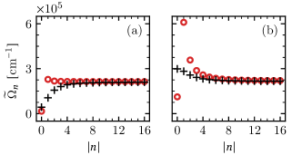
Figure 1: Scaled ring-polymer normal-mode vibrational frequencies for a harmonic potential with frequency (a) $\Omega=500~{}\mathrm{cm}^{-1}$ and (b) $\Omega=3500~{}\mathrm{cm}^{-1}$, calculated at a temperature $T=300~{}$\mathrm{K}$$ for a ring polymer of $N=32$ beads, with $\gamma=32$. The red circles correspond to frequencies that have been scaled according to the original AQCMD scheme (Eq. (18) for $n\neq 0$ and $\kappa_{n}=\gamma$ for $n=0$). The black crosses correspond to the modified scaling of Eq. (20) with $\Omega_{\text{ref}}=2500~{}\mathrm{cm}^{-1}$.

IV.2 Revised spectra for liquid water and ice

The QCMD spectra simulated using the new $\mathbf{I}^{-1}\overline{\bm{\tau}}$ estimator for qTIP4P/F liquid water at $300~{}$\mathrm{K}$$ and ice I_h at $150~{}$\mathrm{K}$$ are shown in Fig. 2, where they are compared with the original QCMD simulations of Ref. 1 and with the results of CMD. The modified mass scaling of Eq. (20) was found to reduce computational cost by a factor of four with respect to the old mass scaling of Eq. (18). The original calculations used a propagation timestep of $0.1/\gamma~{}$\mathrm{f}\mathrm{s}$$ with $\gamma=32$ at 300 K and $\gamma=128$ at 150 K, whereas the new calculations used a timestep of $0.2/\gamma~{}$\mathrm{f}\mathrm{s}$$ with $\gamma=16$ and $64$ at 300 and 150 K respectively. As well as changing the mass scaling, we also re-ordered the steps in the AQCMD propagator from the OBABO splitting of Ref. 1 (where O B A refer to the thermostat, momentum update and position update steps of the velocity Verlet propagator) to BAOAB,[43, 44, 45] which was found to improve numerical stability.

Most of the other simulation details remained the same as in Ref. 1. For both water and ice I_h, the simulations were initialised using eight ring-polymer configurations that were independently pre-equilibrated following standard PIMD procedure. The initial water configurations were then propagated for 50 ps using the AQCMD algorithm. The ice configurations were first thermalised for 1 ps, with a local Langevin thermostat acting on the quasicentroids; this was followed by a 5 ps production run using a global quasicentroid Langevin thermostat;[46] the thermalisation–production cycle was then repeated another four times. The IR absorption spectra were calculated from the average quasicentroid dipole-derivative time-correlation function, following Appendix A of Ref. 1.

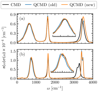
Figure 2: Simulated infrared absorption spectra for the qTIP4P/F PES[17] for (a) liquid water at 300 K and (b) ice I_h at 150 K, showing the difference made by replacing the quasicentroid torque estimator of Ref. 1 (old) with the new estimator of Sec. III (new). The insets show a magnified view of the libration bands, spanning the 250–1000 $\mathrm{cm}^{-1}$ and 500–1000 $\mathrm{cm}^{-1}$ regions in panels (a) and (b) respectively. The CMD and QCMD libration bands become practically identical when the revised QCMD torques are used.

Figure 2 shows that use of the new $\mathbf{I}^{-1}\overline{\bm{\tau}}$ estimator has eliminated the artificial 25 cm^-1 red shift from the QCMD libration bands at both temperatures, which now overlap almost exactly with CMD. At higher frequencies the original and revised QCMD spectra are identical to within statistical uncertainty, except for the intensity of the OH stretch ($\approx 3500~{}\mathrm{cm}^{-1}$) at 300 K, which has increased slightly in the revised spectrum; this brings the intensity ratio of the HOH bend and the OH stretch more in line with those observed in classical MD and CMD calculations at the same temperature.[2] For these reasons, we believe that the new $\mathbf{I}^{-1}\overline{\bm{\tau}}$ estimator gives a better approximation to the exact torque on the molecule quasicentroids than the old estimator of Ref. 1.

IV.3 Radial distribution functions

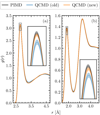
Figure 3: Simulated (a) oxygen-oxygen (O–O) and (b) oxygen-hydrogen (O–H) radial distribution functions (RDFs) for qTIP4P/F water at 300 K, calculated using the old and new quasicentroid torque estimators and standard PIMD. The QCMD results are given for an adiabatic separation of $\gamma=32$ with 32 replicas. The insets show the portion of the first RDF peak highlighted by the grey box.

To consolidate this last statement, we also extracted the (static) O–H and O–O radial distribution functions (RDFs) from the QCMD calculations at $300~{}$\mathrm{K}$$, and compared them with those computed using the old estimator of Ref. 1 and standard PIMD (Fig. 3). Pleasingly, the new estimator reduces the small errors in the radial distribution functions, which now follow the PIMD results very closely.

More broadly, these RDF results show that purely static properties are sufficiently sensitive to the torque estimators that they can be used to verify (independently of the heuristic derivation of Sec. III) which estimator gives a better description of the torque on the quasicentroids. This property should be useful when extending QCMD to treat condensed-phase systems other than pure water.

V Conclusions

The QCMD calculations of Ref. 1, which use the old estimator for $\overline{\bm{\tau}}$, have already given very promising results, yielding infrared spectra for qTIP4P/F water and ice which eliminate most of the artefacts in the stretch region associated with CMD and (T)RPMD. However, it is reassuring that the one minor anomaly in these spectra, namely the 25 cm^-1 red shift of the librational bands, is removed by using the improved estimator presented here, bringing this (essentially classical) region of the spectrum in line with the results of CMD, (T)RPMD and classical MD calculations.

It is also useful that we have been able to speed up the AQCMD algorithm by a factor of four using the modified ‘i-PI’ mass scaling of Sec. IV.1. However, even with this gain in efficiency, AQCMD remains very costly: it is twice as expensive as adiabatic CMD for qTIP4P/F liquid water at 300 K and eight times for ice at 150 K. Another drawback of QCMD is that it requires the internal quasicentroid coordinates to be tailored to each system and is thus tricky to generalise. Nevertheless, recent developments, especially of the fast QCMD method (f-QCMD),[4] suggest that QCMD is likely to become a powerful method for computing infrared spectra in the condensed phase, provided the dynamics do not involve strongly anharmonic ‘floppy’ motion such as in protonated water clusters.[47] We hope that the calculations presented here will serve as useful benchmarks for these and related[48] future developments.