SRIBO: An Efficient and Resilient Single-Range and Inertia Based Odometry for Flying Robots

Abstract

Positioning with one inertial measurement unit and one ranging sensor is commonly thought to be feasible only when trajectories are in certain patterns ensuring observability. For this reason, to pursue observable patterns, it is required either exciting the trajectory or searching key nodes in a long interval, which is commonly highly nonlinear and may also lack resilience. Therefore, such a positioning approach is still not widely accepted in real-world applications. To address this issue, this work first investigates the dissipative nature of flying robots considering aerial drag effects and re-formulates the corresponding positioning problem, which guarantees observability almost surely. On this basis, a dimension-reduced wriggling estimator is proposed accordingly. This estimator slides the estimation horizon in a stepping manner, and output matrices can be approximately evaluated based on the historical estimation sequence. The computational complexity is then further reduced via a dimension-reduction approach using polynomial fittings. In this way, the states of robots can be estimated via linear programming in a sufficiently long interval, and the degree of observability is thereby further enhanced because an adequate redundancy of measurements is available for each estimation. Subsequently, the estimator’s convergence and numerical stability are proven theoretically. Finally, both indoor and outdoor experiments verify that the proposed estimator can achieve decimeter-level precision at hundreds of hertz per second, and it is resilient to sensors’ failures. Hopefully, this study can provide a new practical approach for self-localization as well as relative positioning of cooperative agents with low-cost and lightweight sensors.

I Introduction

Inertial measurement units (IMUs) and ranging sensors such as ultra-wideband radios (UWBs) are lightweight and low-cost [nguyenNTUVIRALVisualinertialranginglidar2021]. Hence, range-inertial odomotry (RIO) with UWBs and IMUs is practically significant for flying robots [xuDecentralizedVisualInertialUWBFusion2020]. More attractively, these sensors are omnidirectional and insusceptible to illumination conditions. The inconvenience is that multiple pre-installed and calibrated anchors are commonly required [muellerFusingUltrawidebandRange2015, caoAccuratePositionTracking2020, jiaCompositeFilteringUWBbased2022]. This hinders autonomous navigation in unknown environments. To tackle this issue, previous researchers attempt to develop localization algorithms using a single UWB anchor [caoAccuratePositionTracking2020, cossetteRelativePositionEstimation2021, wangSingleBeaconBasedLocalization2016], which is referred as a single-ranging problem in this work. As such algorithms only need to fuse an IMU with a single UWB ranging measurement, pre-installation and calibration of anchors are no longer required. However, only using the IMU and UWB range measurements at a single time instance is insufficient to determine the position of a robot, and a sliding windows filtering (SWF) associated with observability analyses are necessary [batistaSingleBeaconNavigation2010]. Such analyses are originated in the field of autonomous underwater vehicles [arrichielloObservabilityAnalysisSingle2015, batistaSingleRangeAided2011], and the results are seamlessly applied for flying robots [caoAccuratePositionTracking2020, cossetteRelativePositionEstimation2021]. Typically, the vehicles or robots are modeled as double-integral systems, and corresponding observability matrices are evaluated either linearly or nonlinearly [arrichielloObservabilityAnalysisSingle2015, indiveriSingleRangeLocalization2016]. These works commonly conclude that the observability is guaranteed only when accumulating actuation in arbitrary two axes is not constant or linearly dependent on each other [arrichielloObservabilityAnalysisSingle2015, cossetteRelativePositionEstimation2021].

Regarding this conclusion, previous researchers attempt to enhance the observability and positioning performance with two approaches. The first one delicately designs controllers to guarantee linearly independent motions in different axes [caoRelativeDockingFormation2020, nguyenDistanceBasedCooperativeRelative2019, nguyenPersistentlyExcitedAdaptive2020]. The second one performs SWF along with observability evaluation [cossetteRelativePositionEstimation2021, shalabyRelativePositionEstimation2021]. As the first approach requires additional control efforts to guarantee positioning performance, this work focuses on the second one.

Existing SWF approaches are commonly nonlinear, and their computational complexity is hyperlinear [cossetteRelativePositionEstimation2021, dongTrajectoryEstimationFlying2022]. Therefore, the sliding window cannot be too long. Unfortunately, a short sliding window may only include small actuation in all the axes, which causes the observability matrix to be ill-conditioned, not to mention the observability itself is not theoretically guaranteed, as discussed already. To address this issue, Ref. [cossetteRelativePositionEstimation2021] tries to perform a key-node selection approach to ehance the observability in an expanded long sliding window. This approach is practically significant, but there are still two aspects requiring further investigation. First, compared to previous research, there is no difference in the observability condition. Therefore, it has to repeatedly compute the observability matrices and their inverse to find proper key nodes, which could be time-consuming [farrellAidedNavigationGPS2008]. Second, the key-node selection is inherently a desampling and has unavoidable information loss. Therefore, it is still necessary to further pursue a computationally efficient and observability guaranteed estimation approach for real-world application [dongTrajectoryEstimationFlying2022].

In view of the state-of-the-art, we propose a framework of single-range and inertia based odometry (SRIBO) to enhance the observability with a refined model considering aerodynamics and improve its efficiency in long sling window with a dimension-reduced linear estimator. First, we refine the model of flying robots considering aerial drag effects, and the single-range inertial odometry (SRIO) merely using an IMU and a UWB is therewith formulated and proven to be observable almost surely. In such a case, it is theoretically guaranteed that one can effectively estimate states taking measurements in an arbitrary horizon. Subsequently, a dimension-reduced wriggling estimator (DWE) is proposed. This estimator slides the estimation horizon in a stepping manner, and output matrices are approximately evaluated based on a sequence of historical estimations. On this basis, we can formulate the optimal state estimation as a batched linear least-square programming. Subsequently, a polynomial fitting approach is introduced to reduce the dimension as well as the computational complexity of the estimation. In this manner, the SRIO can estimate states in a sufficiently long interval with redundant measurements, which further improves the robustness of the estimation. The SRIO is also demonstrated to able to fuse with an additional optical flow sensor, and a so-called single-range, inertia, and optical-flow odometry (SRIFO) is performed. The optical flow sensor provides additional velocity measurements to enhance the estimation performance further, yet failures of such measurements will not lead to singular solutions. Theoretically, both the SRIO and SRIFO in our SRIBO framework are proven to be numerically stable, asymptotic converging and fault-tolerant to sensor failures. Real-time experiments are conducted at last to verify the declarations of observability, computational efficiency, and resilience.

The main contributions are two aspects: 1) modeling with aerial drag effects, the flying robot positioning with SRIBO algorithms is first formulated to be observable almost surely; 2) owing to its efficiency and resilience, the proposed linear DWE can perform estimation in a sufficiently long interval with redundant measurements, which enhances the degree of observability as well as the estimation performance.

II Related work

II-A Single-Range and Inertia based Odometry

The single-range and inertia based odometry has been first considered for the positioning of underwater robots [rossRemarksObservabilitySingle2005, batistaSingleBeaconNavigation2010, ferreiraSingleBeaconNavigation2010]. Practical implementations with Doppler anemometers measuring velocities are also investigated by subsequent researchers [hinsonPathPlanningOptimize2013, wangOptimizationBasedMoving2014]. These positioning approaches are then seamlessly applied for flying robots, e.g., Ref. [nguyenSingleLandmarkDistanceBased2020] uses optical flow sensors measuring velocity alongside a UWB and an IMU. Compared to underwater robots using Doppler anemometers [hinsonPathPlanningOptimize2013, arrichielloObservabilityMetricUnderwater2013, wangOptimizationBasedMoving2014], the performance of positioning with optical flow sensors may deteriorates with varying illumination or insufficient environmental textures [xuOmniSwarmDecentralizedOmnidirectional2022]. Therefore, an effective positioning approach only using measurements from a UWB and an IMU is still essential to guarantee the robustness of the whole system [cossetteRelativePositionEstimation2021, shalabyRelativePositionEstimation2021]. Besides, such a positioning approach with minimal hardware configuration is practically significant for the relative localization of multiple robots [hanIntegratedRelativeLocalization2019].

When lacking directly measured velocities, it is promising to introduce derived velocity from the IMU and UWB measurements to improve the positioning performance. For example, in Ref. [caoAccuratePositionTracking2020], the linear velocity is evaluated to improve positioning precision in a two-dimensional space. Because such an estimation is not precise in more general three-dimensional cases, proper geometric constraints are alternatively imposed in subsequent research regarding the dynamics or kinematics of the robot. For example, position and noise constraints are introduced in Ref. [wangSingleBeaconBasedLocalization2016]. Inherently, position constraints suppress the velocity estimation errors, which further refine the position estimation performance itself [wangSingleBeaconBasedLocalization2016]. To directly constrain the velocity divergence, Ref. [dongTrajectoryEstimationFlying2022] introduces derived constraints to avoid state divergence. Unfortunately, the effectiveness of the derived velocity constraints has not been investigated mathematically, and it should be studied with observability analysis.

II-B Observability based Estimation

In accumulated studies, observability analyses have been either carried out with a classical linearization procedure [batistaSingleBeaconNavigation2010, batistaSingleRangeAided2011, indiveriSingleRangeLocalization2016], or derived from modern control theories [rossRemarksObservabilitySingle2005, arrichielloObservabilityAnalysisSingle2015, berkaneNonlinearNavigationObserver2021]. Such research commonly concludes that the observability can only be guaranteed when the accumulated excitation is linearly independent on different axes [caoAccuratePositionTracking2020]. Regarding this conclusion, an active control approach with exponential convergence is proposed in Ref. [nguyenDistanceBasedCooperativeRelative2019], which persistently excites trajectories to guarantee the observability. Similarly, an integrated estimation-control scheme is proposed to achieve asymptotic convergence in the formation control [caoRelativeDockingFormation2020]. Although the aforementioned active control strategies demonstrate their effectiveness, extra control efforts apart from their primary control objectives are commonly required to guarantee the observability.

As an alternative, recent studies have attempted to iteratively select key nodes, which ensures observability in a long sliding window, to improve the state estimation performance [cossetteRelativePositionEstimation2021]. This is intrinsically a state augmentation approach [ferreiraSingleBeaconNavigation2010], which introduces auxiliary state variables deduced by a combination of concurrent states and/or historical states to enhance the degree of observability [shenQuantifyingObservabilityAnalysis2018]. However, this sliding window filtering approach is highly nonlinear and searching observability-guaranteed key-nodes is also time-consuming [farrellAidedNavigationGPS2008].

Notably, employing velocity measurements can be also viewed to enhance the observability with extra hardware. As discussed previously, this approach has been verified by underwater robots equipped with Doppler anemometers [hinsonPathPlanningOptimize2013, wangOptimizationBasedMoving2014] and flying robots equipped with optical flow sensors [nguyenSingleLandmarkDistanceBased2020]. In the cooperative positioning of flying robots, the UWB and IMU based state estimation is also enhanced with velocity measurements from optical flow sensors [guoUltraWidebandOdometryBasedCooperative2020, guoUltrawidebandBasedCooperative2017]. In a similar manner, visual odometry is included in Refs. [nguyenTightlycoupledUltrawidebandaidedMonocular2020, nguyenFlexibleResourceEfficientMultiRobot2022, nguyenRangeFocusedFusionCameraIMUUWB2021, zhengUWBVIOFusionAccurate2022a]. More comprehensively, an omnidirectional visual–inertial–UWB framework is further proposed for aerial swarm [xuOmniSwarmDecentralizedOmnidirectional2022]. Compared to these implementations with optical sensors, the SRIO has a minimal hardware configuration and is still worth furhter investigation.

II-C Sliding Window Filtering

The SWF, also named as the moving horizon estimation (MHE) [raoConstrainedLinearState2001, wynnConvergenceGuaranteesMoving2014], is an optimal state estimation approach using a sliding window of measurements in each time step [dong-siMotionTrackingFixedlag2011]. Its effectiveness and robustness have been well investigated [raoConstrainedStateEstimation2003, wynnConvergenceGuaranteesMoving2014], and it is also experimentally verified that its performance is better than that of the classical Kalman filter [haseltineCriticalEvalationExtended2005]. For this reason, the single-range based positioning system is commonly developed in an SWF manner [cossetteRelativePositionEstimation2021, shalabyRelativePositionEstimation2021]. Unfortunately, because of the nonlinearity of the optimization, the computational complexity increases hyperlinearly with the size of the sliding window, which may correlate with the degree of observability. Although the key-node selection approach can reduce the states required to estimate in a long sliding window [cossetteRelativePositionEstimation2021], it has to iteratively estimate the observability condition, and the computational cost is still considerable. To tackle this issue, a gradient-aware approach to enhance the computational efficiency is proposed in Ref. [dongTrajectoryEstimationFlying2022]. The divergence is also avoided with velocity penalty. However, this approach is not well formulated in a mathematical manner, and it still cannot well handle a long window of estimation.

When extra sensors, e.g., camera, visual-inertial odometry (VIO), etc, are included alongside the UWB [xuDecentralizedVisualInertialUWBFusion2020, nguyenFlexibleResourceEfficientMultiRobot2022], as the observability is commonly not considered as a main issue ignoring sensor failures, the sliding window size and the computational efficiency have been not well considered in existing work [zhangAgileFormationControl2022a, nguyenRangeFocusedFusionCameraIMUUWB2021, zieglerDistributedFormationEstimation2021].

III Preliminaries

III-A Notations

In this work, $\boldsymbol{0}_{m\times r}$ denotes a zero matrix with dimension $m\times r$. For simplicity, $\boldsymbol{0}_{n}$ denotes a square matrix $\boldsymbol{0}_{n\times n}$. Similarly, $\boldsymbol{I}_{n}$ denotes an identity matrix with dimension $n\times n$. We may further omit the subscript when there is no ambiguity. For a matrix $\boldsymbol{A}$, $\boldsymbol{A}_{ij}$ denotes the element in the $i$th row and $j$th column. $\boldsymbol{A}_{i}$ denotes the vector from $i$th column of $\boldsymbol{A}$. $\boldsymbol{A}_{[i_{1}:i_{2},j_{1}:j_{2}]}$ denotes a block matrix with elements extracted from $i_{1}$th to $i_{2}$th rows and $j_{1}$th to $j_{2}$th columns in matrix $\boldsymbol{A}$. A diagonal matrix is denoted as $\boldsymbol{D}=\operatorname{diag}(\boldsymbol{d})$, with all elements zeros except $\boldsymbol{D}_{ii}=\boldsymbol{d}_{i}$. The integer number set is denoted as $\mathbb{Z}$, and the natural number set is denoted as $\mathbb{N}$, which is equivalent to the positive integer number set $\mathbb{Z}_{+}$. A number $x$ is said to belong to $\mathbb{N}_{>N}$ when $x,N\in\mathbb{N}$ and $x>N$. Similarly, $x\in\mathbb{N}_{\geq N}$ when $x,N\in\mathbb{N}$, and $x\geq N$. A number $x$ is said to belong to $\mathbb{N}_{[N_{1},N_{2}]}$ when $x,N_{1},N_{2}\in\mathbb{N}$ and $N_{1}\leq x\leq N_{2}$.

The flying robot is supposed to fly in a $d$-dimensional space ($d\in\mathbb{N}_{>1}$). We use $\hat{\boldsymbol{x}}$ and $\bar{\boldsymbol{x}}$ to denote the estimation and measurement, respectively, of any state variable $\boldsymbol{x}$ of the robot. we further use $\boldsymbol{x}_{i}$ to index the $i$th element of $\boldsymbol{x}$. Meanwhile, $\boldsymbol{x}_{\langle{i}\rangle}$ is adopted to denote the value of $\boldsymbol{x}$ at some time instant $i$ or $t_{i}$. Combinationally, $\boldsymbol{{x}}_{j\langle{i\rangle}}$ represents the value of $\boldsymbol{x}_{j}$ at instant $i$ or $t_{i}$. A sequence of states continuously sampled at a certain time interval is abbreviated as $\boldsymbol{x}_{\langle{[{k_{1}:k_{2}}]}\rangle}\triangleq\{{\boldsymbol{x}}\}_{k_{1}}^{k_{2}}\triangleq\{\boldsymbol{x}_{\langle{k_{1}}\rangle},\boldsymbol{x}_{\langle{k_{1}+1}\rangle},\cdots,\boldsymbol{x}_{\langle{k_{2}}\rangle}\}$.

III-B Multirotor Flying Robots with Aerial Drags

In this section, we first investigate the observability of a multirotor flying robot considering aerial drag effects. As investigated by Refs. [martinTrueRoleAccelerometer2010a, leishmanQuadrotorsAccelerometersState2014, svachaImprovingQuadrotorTrajectory2017a], a linear drag force equation is adequate to formulate such effects. That is, $\boldsymbol{f}_{D}=-m\boldsymbol{\mu}\boldsymbol{v}$, where $\boldsymbol{f}_{D}$ is the drag force, $m$ is the mass of the robot, $\boldsymbol{v}$ is the velocity vector, and $\boldsymbol{\mu}$ is a diagonal matrix representing the drag coefficients in different directions.

Taking the ranging odometry as the output, the state space representation of the SRIO problem is written as follows

$$\left\{\begin{array}[]{l}\dot{\boldsymbol{x}}=\left[\begin{array}[]{ll}\mathbf{0}_{d}&\boldsymbol{I}_{d}\\ \mathbf{0}_{d}&-\boldsymbol{\mu}\end{array}\right]\boldsymbol{x}+\left[\begin{array}[]{c}\mathbf{0}_{d}\\ \boldsymbol{I}_{d}\end{array}\right]\boldsymbol{u}+\boldsymbol{n_{x}}\\ y=h(\boldsymbol{x})=\frac{1}{2}\|\boldsymbol{p}\|^{2}+{n_{y}}\end{array}\right.$$ (1)

where $\boldsymbol{n_{x}}$ is the process noise, ${n_{y}}$ is the measurement noise, $\boldsymbol{p}$ is the position of the robot, $\boldsymbol{x}=[{\boldsymbol{p}}^{\top},{\boldsymbol{v}}^{\top}]^{\top}$, and $\boldsymbol{u}$ is a $d\times 1$ input vector which physically corresponds to the acceleration of the flying robots.

If an additional optical flow sensor is available, one can further introduce the velocity of the robot into the measurement and implement an SRIFO system, and the state space representation is re-formulated as

$$\left\{\begin{array}[]{l}\dot{\boldsymbol{x}}=\left[\begin{array}[]{ll}\mathbf{0}_{d}&\boldsymbol{I}_{d}\\ \mathbf{0}_{d}&-\boldsymbol{\mu}\end{array}\right]\boldsymbol{x}+\left[\begin{array}[]{c}\mathbf{0}_{d}\\ \boldsymbol{I}_{d}\end{array}\right]\boldsymbol{u}+\boldsymbol{n_{x}}\\ \boldsymbol{y}=\boldsymbol{h}(\boldsymbol{x})=[\frac{1}{2}\|\boldsymbol{p}\|^{2},{\boldsymbol{v}}^{\top}]^{\top}+\boldsymbol{n_{y}}\end{array}\right.$$ (2)

Either Eq. (1) or Eq. (2) can be abstractly described with the following compact form

$$\dot{\boldsymbol{x}}=\boldsymbol{f}(\boldsymbol{x},\boldsymbol{u})+\boldsymbol{n_{x}},\ \boldsymbol{y}=\boldsymbol{h}(\boldsymbol{x})+\boldsymbol{n_{y}}$$ (3)

Remark 1

In practice, a state estimator is commonly implemented independently from the controller. For the sake of convenience, the control input variable $\boldsymbol{u}$ can be evaluated from the measurement of the IMU.

The aforementioned SRIBO systems are nonlinear, they are locally weakly observable only if the observability matrix

$$\mathcal{O}^{\top}:=[\nabla\mathcal{L}_{\boldsymbol{f}}^{0}\boldsymbol{h},\nabla\mathcal{L}_{\boldsymbol{f}}^{1}\boldsymbol{h},\cdots,\nabla\mathcal{L}_{\boldsymbol{f}}^{k}\boldsymbol{h}]$$ (4)

is full rank [hermannNonlinearControllabilityObservability1977a]. Here $\nabla$ denotes the gradient operator and $\mathcal{L}_{\boldsymbol{f}}^{\alpha}\boldsymbol{h}$ is the set of the $\alpha$-order Lie derivatives. Specifically, $\mathcal{L}_{\boldsymbol{f}}^{\alpha}\boldsymbol{h}=\nabla[\mathcal{L}_{\boldsymbol{f}}^{\alpha-1}\boldsymbol{h}]\cdot\boldsymbol{f}$, and $\mathcal{L}_{\boldsymbol{f}}^{0}\boldsymbol{h}=\boldsymbol{h}$.

IV Dimension-reduced Wriggling Estimator

In this section, the DWE is proposed to efficiently estimate states of SRIBO systems. We first derive this approach considering the SRIO problem and then extend it to the SRIFO problem. Its numeric stability, convergence, and fault-tolerance properties are also theoretically investigated.

IV-A The DWE for the SRIO

IV-A1 Observability Analysis

When formulated with the aerial drag effects, the observability of an SRIO system is guaranteed by the following theorem.

Theorem 1

The SRIO system described with Eq. (1) is locally weakly observable almost surely.

Proof:

According to the condition stated in Eq. (4), the observability matrix of Eq. (1) is written as

$$\small\mathcal{O}=\left[\begin{array}[]{cc}{\boldsymbol{p}}^{\top}&\boldsymbol{0}_{1\times d}\\ {\boldsymbol{v}}^{\top}&{\boldsymbol{p}}^{\top}\\ (\boldsymbol{u}-\boldsymbol{\mu}\boldsymbol{v})^{\top}&(2\boldsymbol{v}-\boldsymbol{\mu}\boldsymbol{p})^{\top}\\ -\boldsymbol{\mu}(\boldsymbol{u}-\boldsymbol{\mu}\boldsymbol{v})^{\top}&(3\boldsymbol{u}-6\boldsymbol{\mu}\boldsymbol{v}+\boldsymbol{\mu}^{2}\boldsymbol{p})^{\top}\\ \boldsymbol{\mu}^{2}(\boldsymbol{u}-\boldsymbol{\mu}\boldsymbol{v})^{\top}&(-10\boldsymbol{\mu}\boldsymbol{u}+14\boldsymbol{\mu}^{2}\boldsymbol{v}-\boldsymbol{\mu}^{3}\boldsymbol{p})^{\top}\\ -\boldsymbol{\mu}^{3}(\boldsymbol{u}-\boldsymbol{\mu}\boldsymbol{v})^{\top}&(25\boldsymbol{\mu}^{2}\boldsymbol{u}-30\boldsymbol{\mu}^{3}\boldsymbol{v}+\boldsymbol{\mu}^{4}\boldsymbol{p})^{\top}\\ \end{array}\right]$$ (5)

the detailed derivation of which is presented in Appendix LABEL:ap:lie_srio.

When denoting $\boldsymbol{\chi_{\mu}}=[{\boldsymbol{p}},{\boldsymbol{v}},{\boldsymbol{u}}-\boldsymbol{\mu}\boldsymbol{v}]^{\top}$, one can have $\mathrm{rank}(\mathcal{O})<2d\iff\boldsymbol{\chi_{\mu}}_{i}\equiv\alpha_{j}\boldsymbol{\chi_{\mu}}_{j}+\alpha_{k}\boldsymbol{\chi_{\mu}}_{k},\boldsymbol{\mu}_{i}\equiv\boldsymbol{\mu}_{j}\equiv\boldsymbol{\mu}_{k}$ ($i,j,k\in[1,d]$). This means only when the position, velocity, and acceleration in one direction is always a linear combination of that in the other two directions, this SRIO system is unobservable. This is hardly seen in real-world autonomous navigation. Therefore, probabilistically $p(\mathrm{rank}(\mathcal{O})=2d)=1$. That is, almost surely the observability matrix in Eq. (5) is full rank, and accordingly the SRIO system is locally weakly observable almost surely. $\square$

Remark 2

It should be mentioned that an absolutely static state $\boldsymbol{v}\equiv\boldsymbol{u}\equiv\boldsymbol{0}$ is also a special unobservable case (viewing the condition $\boldsymbol{\chi_{\mu}}_{i}\equiv\alpha_{j}\boldsymbol{\chi_{\mu}}_{j}+\alpha_{k}\boldsymbol{\chi_{\mu}}_{k},\boldsymbol{\mu}_{i}\equiv\boldsymbol{\mu}_{j}\equiv\boldsymbol{\mu}_{k}$). Although we cannot find an absolutely static flying robot in real-flights, but quasi-static states are possibly observed. Apparently, when flying robots in quasi-static state, the condition number of the observability matrix significantly increases. Therefore, the estimation performance will highly correlate with flight velocities and accelerations near quasi-static scenarios.

Remark 3

If the aerial drag force is not included, i.e., $\boldsymbol{\mu}\equiv\boldsymbol{0}$, the observability matrix is formulated as

$${\mathcal{O}}^{\top}=\left[\begin{array}[]{cccccc}\boldsymbol{p}& \boldsymbol{v}&\boldsymbol{u}&\boldsymbol{0}_{n\times 1}& \boldsymbol{0}_{n\times 1}&\boldsymbol{0}_{n\times 1}\\  \boldsymbol{0}_{n\times 1}&\boldsymbol{p}&2\boldsymbol{v}&3\boldsymbol{u}& \boldsymbol{0}_{n\times 1}& \boldsymbol{0}_{n\times 1}\\ \end{array}\right]$$ (6)

which is rank deficiency, i.e., $\mathrm{rank}({\mathcal{O}})\leq 4$. This is why accumulating works commonly conclude that the SRIO system is not locally weakly observable [arrichielloObservabilityAnalysisSingle2015].

Although the SRIO system is observable almost surely, the degree of observability may vary significantly in real-time applications. In particular, when the motion pattern of one direction is closely linearly dependent on that of the other directions, the observability matrix $\mathcal{O}$ is ill-conditioned, which will further lead to estimation performance deterioration. For this reason, we further develop the DWE ensuring numeric stability.

IV-A2 DWE

For a convenient implementation, we re-write the the observation model in Eq. (1) as $y=\|\boldsymbol{p}\|+n_{y}$. Subsequently, neglecting noise terms, a discrete model can be formulated by linearizing with a sampling period $\mathrm{d}t$

$$\left\{\begin{array}[]{l}\boldsymbol{x}_{\langle{k+1}\rangle}=\boldsymbol{A}_{\langle{k}\rangle}\boldsymbol{x}_{\langle{k}\rangle}+\boldsymbol{B}_{\langle{k}\rangle}\boldsymbol{u}_{\langle{k}\rangle}\\ y_{\langle{k+1}\rangle}=\boldsymbol{C}_{\langle{k+1}\rangle}\boldsymbol{x}_{\langle{k+1}\rangle}\end{array}\right.$$ (7)

with $\boldsymbol{A}_{\langle{k}\rangle}=\left[\begin{array}[]{ll}\boldsymbol{I}_{d}&\mathrm{d}t\boldsymbol{I}_{d}\\ \mathbf{0}_{d}&\boldsymbol{I}_{d}-\mathrm{d}t\boldsymbol{\mu}\end{array}\right]$, $\boldsymbol{B}_{\langle{k}\rangle}=\left[\begin{array}[]{c}\frac{1}{2}\mathrm{d}t^{2}\\ \mathrm{d}t\\ \end{array}\right]\otimes\boldsymbol{I}_{d}$, and $\boldsymbol{C}_{\langle{k}\rangle}=[\boldsymbol{p}^{\top}_{\langle{k}\rangle}/\|\boldsymbol{p}_{\langle{k}\rangle}\|,\boldsymbol{0}_{1\times d}]$. Because both $\boldsymbol{A}_{\langle{k}\rangle}$ and $\boldsymbol{B}_{\langle{k}\rangle}$ are time invariant for some fixed $\mathrm{d}t$, we use abbreviations $\boldsymbol{A}\triangleq\boldsymbol{A}_{\langle{k}\rangle}$ and $\boldsymbol{B}\triangleq\boldsymbol{B}_{\langle{k}\rangle}$ in the following formulation when without confusion.

On this basis, the DWE $\mathcal{D_{W}}$ is implemented and conceptually illustrated in Fig. 1. Upon each period $\mathcal{T}_{\langle{i+1}\rangle}$, we aim to perform a maximum a posteriori estimate of the state sequence $\{\hat{\boldsymbol{x}}\}_{1}^{k}$ based on the input $\{\boldsymbol{u}\}_{0}^{k-1}$, the range measurement $\{\bar{r}\}_{1}^{k}$, and a prior estimate $\{\hat{\boldsymbol{x}}^{-}\}_{0}^{k-1}$ which is equivalent to the posteriori estimation $\{\hat{\boldsymbol{x}}\}_{1}^{k}$ in previous period $\mathcal{T}_{\langle{i}\rangle}$. Mathematically, this estimator is implemented as follows in an interval with $k_{w}+1\ (k_{w}\in\mathbb{N}_{>2d})$ sampling points

$$\hat{\boldsymbol{x}}=\arg\min_{\boldsymbol{x}}J=\sum_{i=0}^{k_{w}-1}c_{1\langle{i}\rangle}+\sum_{i=1}^{k_{w}}c_{2\langle{i}\rangle}+\sum_{i=1}^{k_{w}}c_{3\langle{i}\rangle}$$ (8)

where $c_{1\langle{i}\rangle}=\boldsymbol{e}_{1\langle{i\rangle}}^{\top}\boldsymbol{P}^{-1}_{\langle{{i}}\rangle}\boldsymbol{e}_{1\langle{i}\rangle}$, $c_{2\langle{i}\rangle}=\boldsymbol{e}_{2\langle{i\rangle}}^{\top}\boldsymbol{Q}^{-1}_{\langle{{i}}\rangle}\boldsymbol{e}_{2\langle{i}\rangle}$, $c_{3\langle{i}\rangle}=\boldsymbol{e}_{3\langle{i\rangle}}^{\top}\boldsymbol{R}^{-1}_{\langle{{i}}\rangle}\boldsymbol{e}_{3\langle{i}\rangle}$, $\boldsymbol{e}_{1\langle{i\rangle}}\triangleq\hat{\boldsymbol{x}}_{\langle{i}\rangle}-\hat{\boldsymbol{x}}_{\langle{i}\rangle}^{-}$, $\boldsymbol{e}_{2\langle{i\rangle}}\triangleq\hat{\boldsymbol{x}}_{\langle{i}\rangle}-\boldsymbol{A}\hat{\boldsymbol{x}}_{\langle{i-1}\rangle}-\boldsymbol{B}{\boldsymbol{u}_{\langle{i-1}\rangle}}$, and $\boldsymbol{e}_{3\langle{i\rangle}}\triangleq\bar{r}_{\langle{i}\rangle}-\boldsymbol{C}_{\langle{i}\rangle}\hat{\boldsymbol{x}}_{\langle{i}\rangle}$. Statistically, $\boldsymbol{P}_{\langle{i}\rangle}$, $\boldsymbol{Q}_{\langle{i}\rangle}$ and $\boldsymbol{R}_{\langle{i}\rangle}$ correspond to the covariance matrices of the state estimate, the process, and the measurement, respectively [dongTrajectoryEstimationFlying2022].

Remark 4

For typical flying robots such as multirotor robots, the input $\boldsymbol{u}_{\langle{i}\rangle}$ equals the instant acceleration $\boldsymbol{a}_{\langle{i}\rangle}$, which can be directly measured by the IMU. The lateral acceleration $\boldsymbol{a}_{x}$ and $\boldsymbol{a}_{y}$ are also closely related to the attitude of the flying robot when the motion is not too aggressive. Specifically, $\boldsymbol{a}_{x}\approx g\sin\theta\approx g\theta$, and $\boldsymbol{a}_{y}\approx-g\sin\phi\approx-g\phi$, where $\theta$ and $\phi$ are the pitch and roll angles [dongHighperformanceTrajectoryTracking2014]. In practice, the attitude estimation precision is higher than that of the directly measured acceleration. Therefore, it is a good choice to evaluate the acceleration based on the attitude estimation.

Denoting $\boldsymbol{E}=[\boldsymbol{e}^{\top}_{1\langle{0}\rangle},\boldsymbol{e}^{\top}_{1\langle{1}\rangle},\cdots,\boldsymbol{e}^{\top}_{1\langle{k_{w}-1}\rangle},\boldsymbol{e}^{\top}_{2\langle{1}\rangle},\boldsymbol{e}^{\top}_{2\langle{2}\rangle},\cdots$, $\boldsymbol{e}^{\top}_{2\langle{k_{w}}\rangle}$, $\boldsymbol{e}^{\top}_{3\langle{1}\rangle},\boldsymbol{e}^{\top}_{3\langle{2}\rangle},\cdots,\boldsymbol{e}^{\top}_{3\langle{k_{w}}\rangle}]$, $\boldsymbol{P}=\operatorname{diag}(\boldsymbol{P}_{\langle{0}\rangle},\boldsymbol{P}_{\langle{1}\rangle}$, $\cdots$, $\boldsymbol{P}_{\langle{k_{w}-1}\rangle})$, $\boldsymbol{Q}=\operatorname{diag}(\boldsymbol{Q}_{\langle{0}\rangle},\boldsymbol{Q}_{\langle{1}\rangle},\cdots,\boldsymbol{Q}_{\langle{k_{w}-1}\rangle})$, $\boldsymbol{R}=\operatorname{diag}(\boldsymbol{R}_{\langle{1}\rangle},\boldsymbol{R}_{\langle{2}\rangle},\cdots,\boldsymbol{R}_{\langle{k_{w}}\rangle})$, and $\boldsymbol{W}=\operatorname{diag}(\boldsymbol{P}^{-1},\boldsymbol{Q}^{-1},\boldsymbol{R}^{-1})$, Eq. (8) can be re-formulated as a batch nonlinear least-squares estimator as follows [barfootStateEstimationRobotics2017]

$$\hat{\boldsymbol{x}}=\arg\min_{\boldsymbol{x}}J=\boldsymbol{E}^{\top}\boldsymbol{W}\boldsymbol{E}$$ (9)

The problem formulated with Eq. (8) or Eq. (9) is general solved with the Gauss-Newton algorithm or its variants [dongTrajectoryEstimationFlying2022, cossetteRelativePositionEstimation2021]. It is time-consuming when the window size, i.e., $k_{w}$, becomes large. Therefore, this work develops an alternative to solve this problem with high efficiency.

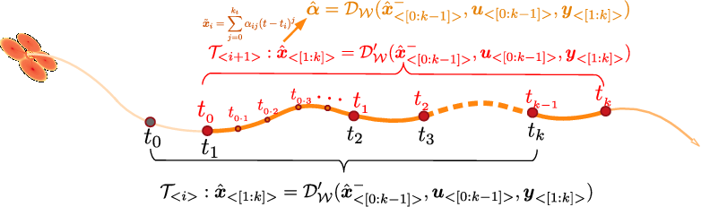
Figure 1: A conceptual illustration of dimension-reduced wriggling estimator

To facilitate this development, based on Eq. (7) and Eq. (8), the matrix $\boldsymbol{E}$ is re-written as

$$\boldsymbol{E}=\begin{bmatrix}\tilde{\boldsymbol{I}}_{A}\\ \tilde{\boldsymbol{A}}\\ \tilde{\boldsymbol{C}}\\ \end{bmatrix}\boldsymbol{x}-\begin{bmatrix}\boldsymbol{I}_{2dk_{w}}&\boldsymbol{0}&\boldsymbol{0}\\ \boldsymbol{0}&\tilde{\boldsymbol{B}}&\boldsymbol{0}\\ \boldsymbol{0}&\boldsymbol{0}&\boldsymbol{I}_{k_{w}}\\ \end{bmatrix}\boldsymbol{\theta}\triangleq\boldsymbol{E_{x}}{\boldsymbol{x}}-\boldsymbol{E_{\theta}}\boldsymbol{\theta}$$ (10)

where $\boldsymbol{x}=[\boldsymbol{x}^{\top}_{\langle{0}\rangle},\boldsymbol{x}^{\top}_{\langle{1}\rangle},\cdots,\boldsymbol{x}^{\top}_{\langle{k_{w}}\rangle}]$, $\boldsymbol{\theta}=[\hat{\boldsymbol{x}}^{-\top}_{\langle{0}\rangle},\hat{\boldsymbol{x}}^{-\top}_{\langle{1}\rangle}$, $\cdots$, $\hat{\boldsymbol{x}}^{-\top}_{\langle{k_{w}-1}\rangle},\boldsymbol{a}^{\top}_{\langle{0}\rangle},\boldsymbol{a}^{\top}_{\langle{1}\rangle},\cdots,\boldsymbol{a}^{\top}_{\langle{k_{w}-1}\rangle},\bar{r}_{\langle{1}\rangle},\bar{r}_{\langle{2}\rangle},\cdots,\bar{r}_{\langle{k_{w}}\rangle}]^{\top}$, $\tilde{\boldsymbol{I}}_{A}=[\boldsymbol{I}_{2dk_{w}},\ \boldsymbol{0}_{2dk_{w}\times 2d}]$, $\tilde{\boldsymbol{A}}$ is a block matrix with $\tilde{\boldsymbol{A}}_{[2di+1:2d(i+1),2di+1:2d(i+2)]}=[-\boldsymbol{A},\ \boldsymbol{I}_{2d}]\ (i\in[0,k_{w}-1])$, $\tilde{\boldsymbol{C}}$ is a block matrix $\tilde{\boldsymbol{C}}_{[i,2di+1:2d(i+1)]}=\boldsymbol{C}_{\langle{i}\rangle}\ (i\in[1,k_{w}])$, and $\tilde{\boldsymbol{B}}$ is a diagonal matrix with $\tilde{\boldsymbol{B}}=\mathrm{diag}([\underbrace{\boldsymbol{B},\boldsymbol{B},\cdots,\boldsymbol{B}}_{k_{w}\times\boldsymbol{B}}])$.

Reasonably, $\boldsymbol{C}_{\langle{i}\rangle}=\boldsymbol{C}_{\langle{i}\rangle}^{-},\ i\in[1,k_{w}-1]^{\top}$, where $\boldsymbol{C}_{\langle{i}\rangle}^{-}$ equals $\boldsymbol{C}_{\langle{i+1}\rangle}$ in previous period. Particularly, $\boldsymbol{C}_{\langle{k_{w}}\rangle}$ can be approximated with $\boldsymbol{C}_{\langle{k_{w}-1}\rangle}$, or we can first evaluate a prior estimate $\tilde{\boldsymbol{x}}_{k_{w}}=\boldsymbol{A}\hat{\boldsymbol{x}}_{k_{w}-1}+\boldsymbol{B}\boldsymbol{u}$, and then evaluate $\boldsymbol{C}_{\langle{k_{w}}\rangle}$ with Eq. (7). On this basis, substituting Eq. (10) into Eq. (9), one can obtain an optimal estimation $\hat{\boldsymbol{x}}$ by taking $\frac{\partial{J}}{\partial\boldsymbol{x}}=0$. An analytical solution to this problem is

$$\hat{\boldsymbol{x}}=(\boldsymbol{E_{x}}^{\top}\boldsymbol{W}\boldsymbol{E_{x}})^{-1}\boldsymbol{E_{x}}^{\top}\boldsymbol{W}\boldsymbol{E_{\theta}}\boldsymbol{\theta}$$ (11)

Lemma 1

Denoting $\boldsymbol{W_{E}}\triangleq\boldsymbol{E_{x}}^{\top}\boldsymbol{W}\boldsymbol{E_{x}}$, if $\boldsymbol{P}_{\langle{i}\rangle}$ and $\boldsymbol{Q}_{\langle{i}\rangle}$ are positive definite, the matrix $\boldsymbol{W_{E}}$ is always invertible and the solution of Eq. (11) exists uniquely.