Violation of Detailed Balance in Quantum Open Systems

Abstract

We consider the dynamics of a quantum system immersed in a dilute gas at thermodynamic equilibrium using a quantum Markovian master equation derived by applying the low-density limit technique. It is shown that the Gibbs state at the bath temperature is always stationary while the detailed balance condition at this state can be violated beyond the Born approximation. This violation is generically related to the absence of time-reversal symmetry for the scattering T matrix, which produces a thermalization mechanism that allows the presence of persistent probability and heat currents at thermal equilibrium. This phenomenon is illustrated by a model of an electron hopping between three quantum dots in an external magnetic field.

I Introduction

Detailed balance at equilibrium (DBE) [1, 2, 3] is a core principle of today´s thermodynamics. It ensures the lack of persistent currents at equilibrium [4] and plays a key role in a wide range of fields, including the Onsager relations [5, 6] and reaction kinetics [7] in chemistry, fluctuation theorems [8, 9, 10, 11, 12] in statistical mechanics, open quantum systems [13, 14] in quantum mechanics, and Kirchhoff’s law [15] in electromagnetism. Detailed balance has been so closely identified with thermal equilibrium [16] that its violation has been used as an indicator of lack of equilibrium [17, 18] and has also been suggested as a measure of distance from equilibrium [19].

The assumption of DBE is prevalent across several fields. But interestingly, it is not actually required by any fundamental law [20]. This was long ago recognized by Onsager [5] himself who brought up the Hall effect as an example where this principle does not hold. Other examples of systems that violate detailed balance include the Michaelis-Menten kinetics for enzyme kinetics [21, 22], totally asymmetric simple exclusion process for one-dimensional transport [23, 24] directed percolation for fluid dynamics [25] and nonreciprocal systems [26, 27, 28]. Many unexpected effects in nonreciprocal materials have been theoretically predicted in the last years: persistent heat currents in thermal equilibrium [29], violations of the Kirchhoff law [28], potential violations of Earnshaw’s theorem [30], deviations from the Green-Kubo relations [31], photon thermal Hall effect [32], giant magnetoresistance for the heat flux [33], and the creation of a Casimir heat engine [34].

Unfortunately, currently used tools are insufficient for developing the microscopic models needed to study the dynamics and thermodynamics of systems that violate DBE. Here, we use the following definition of DBE

$$a_{k\ell}e^{-\beta\mathcal{E}_{\ell}}=a_{\ell k}e^{-\beta\mathcal{E}_{k}},$$ (1)

where $a_{k\ell}$ are transition rates between microstates of the system with energies $\mathcal{E}_{k},\mathcal{E}_{\ell}$ and $\beta$ is the inverse temperature of the bath. The Gorini, Kossakowski, Lindblad and Sudarshan (GKLS) [35, 36] equation derived at the weak coupling limit [37] cannot be used because it automatically complies with DBE (see Ref. [38] and section III). The lack of microscopic models has resulted in contradicting statements in the literature regarding basic thermodynamic properties, such as the possibility of reaching thermal equilibrium [27, 39, 40, 41, 42] and the divergence of entropy production [43, 44, 45, 46, 47].

To clarify the thermodynamic properties of systems that violate DBE, we use a GKLS master equation in the low density limit (LDL) [48] which can lead into the violation of DBE. We note that the notion of DBE is not restricted to this limit and it will be interesting to study its violation beyond this regime. We prove that despite the violation of DBE, fundamental thermodynamic behavior still holds: the reduced system reaches thermal equilibrium, at which the entropy production is zero. Nevertheless, DBE violation produces a different thermalization mechanism that allows persistent probability and heat currents at thermal equilibrium. To exemplify these effects we study a toy model for a single electron tunneling between three quantum dots in the presence of a magnetic field.

II Quantum Master Equations at low density limit

We consider a quantum system $S$ with a discrete spectrum physical Hamiltonian, $H_{S}=\sum_{k}\mathcal{E}_{k}|k\rangle\langle k|,$ immersed in an ideal bosonic or fermionic gas of free (quasi-) particles at a thermal equilibrium state given by the inverse temperature $\beta$ and particle density $\nu$. The derivation of the dynamics for the reduced density matrix is performed under the assumption that the density of gas particles is low. As shown in Ref. [48] this assumption implies that the form of the master equation does not depend on particle statistics and is fully determined by the scattering of a single particle by the system $S$. Therefore, it is sufficient to determine the Hamiltonian $H_{tot}$ of the system composed of $S$ and a single particle, $H_{tot}=H_{S}+H_{P}+H_{int}.$ We assume for simplicity that the gas particle is spinless and is described by its Hamiltonian $H_{P}$ in momentum representation,

$$H_{P}=\int d\mathbf{p}\,E_{\mathbf{p}}|\mathbf{p}\rangle\langle\mathbf{p}|,\quad\langle\mathbf{p}|\mathbf{p}^{\prime}\rangle=\delta(\mathbf{p}-\mathbf{p}`).$$ (2)

The state of the gas is described by the single-particle probability distribution in momentum space $G(\mathbf{p})$.

The single-particle scattering Møller wave operator is defined as [49]

$$\Omega_{+}=\lim_{t\to\infty}e^{-iH_{tot}t}e^{i(H_{S}+H_{P})t},$$ (3)

and its superoperator version is $\Gamma_{+}=\Omega_{+}\cdot\Omega_{+}^{\dagger}$. The $T$ operator is the main mathematical object describing the scattering process and is defined as

$$T=H_{int}\Omega_{+}.$$ (4)

It produces a family of transition operators acting on the Hilbert space of $S$ and labeled by the Bohr frequencies of $H_{S}$ denoted by $\{\omega\}$ and pairs of the particle’s momenta,

$$T_{\omega}(\mathbf{p}^{\prime},\mathbf{p})=\sum_{\mathcal{E}_{k}-\mathcal{E}_{\ell}=\omega}\langle k,\mathbf{p}^{\prime}|T|\mathbf{p},\ell\rangle|k\rangle\langle\ell|.$$ (5)

We further assume that the dilute ideal gas is at a stationary state fully characterized by the probability distribution in momentum space $G(\mathbf{p})$ and the particle density $\nu$. As proven in Ref. [48] the reduced dynamics of $S$ is governed by the following quantum master equation (QME)

$$\frac{d}{dt}\rho_{S}=-i[H_{S},\rho_{S}]+\mathcal{L}\rho_{S},$$ (6)

where the dissipative generator is

$$\mathcal{L}\rho_{S}=\nu\pi\sum_{\omega}\int d\mathbf{p}\int d\mathbf{p}^{\prime}\,G(\mathbf{p})\delta(E_{\mathbf{p}^{\prime}}-E_{\mathbf{p}}+\omega)\times$$

$$\bigl{\{}[T_{\omega}(\mathbf{p}^{\prime},\mathbf{p})\rho_{S},T^{\dagger}_{\omega}(\mathbf{p}^{\prime},\mathbf{p})]+[T_{\omega}(\mathbf{p}^{\prime},\mathbf{p}),\rho_{S}T^{\dagger}_{\omega}(\mathbf{p}^{\prime},\mathbf{p})]\bigr{\}}.$$ (7)

$\mathcal{L}$ can be expressed in the form of an ergodic average

$$\mathcal{L}=\lim_{a\to\infty}\frac{1}{a}\int_{0}^{a}dte^{it[H_{S},\cdot]}\mathcal{L}_{0}\,e^{-it[H_{S},\cdot]},$$ (8)

where $\mathcal{L}_{0}$ is given by

$$\mathcal{L}_{0}\rho_{S}=-i\int d\mathbf{p}\,\langle\mathbf{p}|[H_{int},\Gamma_{+}(\rho_{S}\otimes\rho_{P})]|\mathbf{p}\rangle.$$ (9)

$\rho_{P}$ is the formal density matrix for the gas particle. This averaging (Eq. (8)) is usually associated with the secular approximation which is a necessary step to assure positivity preserving of the derived QME.

The basic properties of the QME given by Eqs. (6) and (7) are the following.

(1) The dissipative generator $\mathcal{L}$ commutes with the Hamiltonian part $-i[H_{S},\cdot]$,

$$\mathcal{L}[H_{S},\cdot]=[H_{S},\cdot]\mathcal{L}.$$ (10)

This implies that populations of $H_{S}$ eigenstates evolve independently of their coherences.

(2) If the gas is at thermal equilibrium at the inverse temperature $\beta$ the probability distribution of the particle’s momenta is given by

$$G(\mathbf{p})=Z^{-1}e^{-\beta E_{\mathbf{p}}}$$ (11)

and the stationary state of the system is the Gibbs state,

$$\rho^{\beta}_{S}=Z_{S}^{-1}e^{-\beta H_{S}}.$$ (12)

(3) Under the additional ergodicity condition, any initial state of the system relaxes to the Gibbs state $\rho_{S}^{\beta}$.

Proofs
Property (1) is a direct consequence of the averaging procedure [Eq. (8)]. Namely, using the following identity, valid for any fixed $\tau$

$$\mathcal{L}=\lim_{a\to\infty}\frac{1}{a}\int_{0}^{a}dte^{i(t+\tau)[H_{S},\cdot]}\mathcal{L}_{0}\,e^{-i(t+\tau)[H_{S},\cdot]}=$$

$$e^{i\tau[H_{S},\cdot]}\mathcal{L}e^{-i\tau[H_{S},\cdot]}$$ (13)

and differentiating both sides of Eq. (13) at $\tau=0$ one obtains Eq. (10).

Property (2) is a new result, as in Ref. [48] it is assumed that the system complies with microreversibility. This implies DBE. Here, we use only the intertwining property of the wave operator $\Omega_{+}$,

$$\Omega_{+}(H_{S}+H_{P})\Omega^{\dagger}_{+}=H_{S}+H_{P}+H_{int}=H_{tot},$$ (14)

or equivalently,

$$\Omega_{+}e^{-\beta(H_{S}+H_{P})}\Omega^{\dagger}_{+}=e^{-\beta H_{tot}}.$$ (15)

$\mathcal{L}\rho_{S}^{\beta}=0$ is obtained by assuming the gas particle is in a thermal state, $\rho_{P}=Z^{-1}e^{-\beta H_{P}}$ and using Eqs.(8), (15) and (9) (below $C$ is an irrelevant constant). $\mathcal{L}\rho_{S}^{\beta}$ is equal to

$$C\lim_{a\to\infty}\frac{1}{a}\int_{0}^{a}dt\,e^{iH_{S}t}\mathrm{Tr}_{P}[H_{int},\Omega_{+}e^{-\beta(H_{S}+H_{P})}\Omega^{\dagger}_{+}]e^{-iH_{S}t}$$ (16)

Using Eq., (15), $H_{int}=H_{tot}-H_{S}-H_{P}$, and the fact that $[H_{tot},e^{-\beta H_{tot}}]=0$ we get

$$C\lim_{a\to\infty}\frac{-1}{a}\int_{0}^{a}dt\,e^{iH_{S}t}\mathrm{Tr}_{P}[H_{S}+H_{P},e^{-\beta H_{tot}}]e^{-iH_{S}t}=$$

$$C\lim_{a\to\infty}\frac{-1}{a}\int_{0}^{a}dt\,[H_{S},e^{iH_{S}t}\mathrm{Tr}_{P}(e^{-\beta H_{tot}})e^{-iH_{S}t}].$$ (17)

In the last equality we have used that the trace of a commutator is zero. Equation (17) can be rewritten as

$$C\lim_{a\to\infty}\frac{-1}{a}\int_{0}^{a}dt\,\frac{d}{dt}\Bigl{(}e^{iH_{S}t}\mathrm{Tr}_{P}(e^{-\beta H_{tot}})e^{-iH_{S}t}\Bigr{)}=C\times$$

$$\lim_{a\to\infty}\frac{-1}{a}\Bigl{\{}e^{iH_{S}a}\mathrm{Tr}_{P}(e^{-\beta H_{tot}})e^{-iH_{S}a}-\mathrm{Tr}_{P}e^{-\beta H_{tot}}\Bigr{\}}=0,$$ (18)

where we use the fact that the numerator has finite norm.

Property (3) is a consequence of the results obtained in Ref. [50].

Properties (1)-(3) show that the Gibbs state is the steady state of the QME obtained in LDL for thermal equilibrium environments (ideal gas) without any additional assumptions such as DBE or microreversibility.

III Detailed balance condition for LDL dynamics

In this section we discuss the sufficient generic conditions leading to the detailed balance condition [Eq. (1)] for QME of the LDL type [Eqs. (6) and(7)]. The analysis is much simpler for the case of an $H_{S}$ with nondegenerated spectrum.

For an $H_{S}$ with a nondegenerated spectrum the diagonal elements of the density matrix, $p_{k}\equiv\langle k|\rho_{S}|k\rangle$, evolve independently from the off-diagonal ones and satisfy the Pauli master equation of the form

$$\frac{d}{dt}p_{k}=\sum_{\ell}\bigl{(}a_{k\ell}\,p_{\ell}-a_{\ell k}\,p_{k}\bigr{)}$$ (19)

with

$$a_{k\ell}=\nu\pi\int d\mathbf{p}\int d\mathbf{p}^{\prime}\,G(\mathbf{p})\delta\bigl{\{}(E_{\mathbf{p}^{\prime}}+\mathcal{E}_{k})-(E_{\mathbf{p}}+\mathcal{E}_{\ell})\bigr{\}}\times$$

$$|\langle k,\mathbf{p}^{\prime}|T|\mathbf{p},\ell\rangle|^{2}.$$ (20)

Using Eq. (20) with $G(\mathbf{p})=Z^{-1}e^{-\beta E_{\mathbf{p}}}$ one derives the following identity

$$a_{k\ell}e^{-\beta\mathcal{E}_{\ell}}=a_{\ell k}e^{-\beta\mathcal{E}_{k}}I(k,\ell),$$ (21)

where

$$I(k,\ell)=$$

$$\frac{\int d\mathbf{p}\int d\mathbf{p}^{\prime}\,e^{-\beta E_{\mathbf{p}}}\delta\bigl{\{}E_{\mathbf{p}^{\prime}}+\omega_{kl}-E_{\mathbf{p}}\bigr{\}}|\langle k,\mathbf{p}^{\prime}|T|\mathbf{p},\ell\rangle|^{2}}{\int d\mathbf{p}\int d\mathbf{p}^{\prime}\,e^{-\beta E_{\mathbf{p}}}\delta\bigl{\{}E_{\mathbf{p}^{\prime}}+\omega_{kl}-E_{\mathbf{p}}\bigr{\}}|\langle\ell,\mathbf{p}|T|\mathbf{p}^{\prime},k\rangle|^{2}}.$$ (22)

Here $\omega_{kl}=\mathcal{E}_{k}-\mathcal{E}_{\ell}$. The DBE condition is satisfied if and only if $I(k,\ell)=1$ for those pairs $(k,\ell)$ for which transition probabilities are nonzero. It may happen incidentally for a particular choice of the parameters, but we discuss only the generic situations which are related to symmetries of the system.

The first sufficient symmetry condition is Hermicity of the $T$ matrix $(T=T^{\dagger})$, that is $\langle k,\mathbf{p}^{\prime}|T|\mathbf{p},\ell\rangle=\overline{\langle\ell,\mathbf{p}|T|\mathbf{p}^{\prime},k\rangle}$. This is always satisfied for the Born approximation where $T\simeq H_{int}$. This approximation is valid at the weak coupling limit where DBE always holds. Physically, at the dilute limit, a hermitian $T$ matrix represents a lossless system [26].

The second sufficient condition is assuming that the T matrix is a symmetric matrix, $\langle k,\mathbf{p}^{\prime}|T|\mathbf{p},\ell\rangle=\langle\ell,\mathbf{p}|T|\mathbf{p}^{\prime},k\rangle$, which implies that the system is reciprocal [27, 26].

The third case corresponds to time-reversal symmetry or microreversibility. It means that the states $|k\rangle$ are invariant with respect to time reversal, $E_{\mathbf{p}}=E_{-\mathbf{p}}$ and the probability of the scattering event $|\ell,\mathbf{p}\rangle\mapsto|k,\mathbf{p}^{\prime}\rangle$ is equal to the probability of time-reversed event $|k,-\mathbf{p}^{\prime}\rangle\mapsto|\ell,-\mathbf{p}\rangle$. This condition means

$$|\langle k,\mathbf{p}^{\prime}|T|\mathbf{p},\ell\rangle|^{2}=|\langle\ell,-\mathbf{p}|T|-\mathbf{p}^{\prime},k\rangle|^{2},$$ (23)

which leads to $I(k,\ell)=1$.

The fourth condition combines time reversal with parity transformation (space inversion) which leads to the condition

$$|\langle k,\mathbf{p}^{\prime}|T|\mathbf{p},\ell\rangle|^{2}=|\langle\ell,\mathbf{p}|T|\mathbf{p}^{\prime},k\rangle|^{2}.$$ (24)

We note here that only on shell processes have to be considered. This is a consequence of the delta function in Eq. (20), which ensures energy conservation. For particular systems it may happen that certain geometric symmetry can restore detailed balance (see a toy model in Section V and Supplementary Information (SI).

The above conditions were derived for the T matrix. Some of them can also be obtained for the Green’s operator (see discussion below Eq S9 on the SI).

Fulfilling at least one of the mentioned conditions, will be enough to ensure DBE. In section V we show a toy model that does not comply with any of the above conditions, resulting in DBE violation (see Section S.2.a on SI).

IV Thermodynamic laws and entropy production

DBE violation provides additional freedom to the reduced dynamics. Nevertheless, the time invariance of the Gibbs state still allows for preserving the fundamental principles of thermodynamics: the impossibility of steady work extraction from a single thermal bath or cooling of a cold bath without an external driving. Mathematically, the LDL master equation (6), satisfies: (i) the zeroth law of thermodynamics [see Eq. (11)], (ii) the first law of thermodynamics (implied by the Hamiltonian model of open system), and (iii) the second law of thermodynamics (implied by the Spohn inequality [3]).

For diagonal density matrices the entropy production defined as

$$\sigma=\sum_{k}\frac{dp_{k}}{dt}[\ln p^{eq}_{k}-\ln p_{k}];\quad p^{eq}_{k}\equiv Z^{-1}e^{-\beta\mathcal{E}_{k}},$$ (25)

can be written in terms of the DBE violation as

$$\sigma=\sum_{k>j}\left[K_{jk}\ln\left(\frac{p_{k}}{p_{j}}\frac{a_{jk}}{a_{kj}}\right)+K_{jk}\ln I(k,j)\right].$$ (26)

where $K_{jk}=a_{jk}p_{k}-a_{kj}p_{j}$ is the probability current from the microstate $\{k\}$ to the microstate $\{j\}$. The first term in Eq. (26) corresponds to the Schnakenberg formulation of entropy production [51] and the second to deviations due to the lack of DBE. Equation (26) is valid for any temporal state as long as the steady state of the dynamics is a Gibbs state [see Eq. (12)] as is the case for Eq. (6).

Furthermore, at thermal equilibrium the second term can be rewritten as

$$\sum_{k>j}a_{jk}p^{eq}_{k}\left[1-I(k,j)\right]\ln I(k,j),$$ (27)

which is always negative. At thermal equilibrium the first and second laws force the entropy production to be zero. Therefore, to compensate for the negativity of Eq. (27), the Schnakenberg entropy production should be positive and increases with the DBE violation: $|1-I(k,j)|$.

V Three-level open system without time-reversal symmetry

As a toy model we consider a single (spinless) electron that can occupy three dots ($1$,$2$,$3$) in an equilateral triangle arrangement in the presence of a magnetic field. The positions of the quantum dots (QD) are given by $\{\mathbf{q}_{j};\iota=1,2,3\}$. This system (3QD) is governed by the single particle Hubbard Hamiltonian. This Hamiltonian type has been used to study more complex systems, such as Benzene molecules [52] and could be used to extend our results to more realistic scenarios. In the single electron localized basis ($|1\rangle,|2\rangle,|3\rangle$), the Hamiltonian is given by

$$H_{el}=\tau\left(\begin{array}[]{ccc}0&e^{-i2\pi\phi/3}&e^{i2\pi\phi/3}\\ e^{i2\pi\phi/3}&0&e^{-i2\pi\phi/3}\\ e^{-i2\pi\phi/3}&e^{i2\pi\phi/3}&0\end{array}\right),$$ (28)

where $\tau$ is the tunneling parameter and $\phi$ is the magnetic flux [3]. The diagonal form of this Hamiltonian is $H_{el}=\sum_{j\in\{\pm,0\}}=\mathcal{E}_{j}|j\rangle\langle j|$ where $\mathcal{E}_{j}=-2|\tau|\cos[2\pi(\phi+j*1)/3]$. For most values of the magnetic flux the Hamiltonian is nondegenerated.

The 3QD interacts with a low-density gas of free particles of mass $m$ that is at a thermal state with inverse temperature $\beta$. We assume a simple form of the interaction potential given by

$$H_{int}(\mathbf{q})=\sum_{\iota\in\{1,2,3\}}V_{\iota}(\mathbf{q}-\mathbf{q}_{\iota})|\iota\rangle\langle\iota|,$$ (29)

where $V_{\iota}(\mathbf{q}-\mathbf{q}_{\iota})$ is a short range repulsive potential between the electron and the particle. In order to simplify numerical calculations we assume that the distance between dots is small in comparison with the typical wavelength of a quantum scatterer. This allows one to treat all dots as sitting at the same point, while keeping the structure of the internal electron Hamiltonian [Eq. (28)]. Then we can replace smooth potentials in Eq. (29) by 1D Dirac deltas ${\cal V}_{\iota}\delta(q)$ and at the same time use as a heat bath a one-dimensional particle gas. Figure 1 shows the results of numerical calculations for this simplified model showing a substantial violation of DBE while the stationary state remains a Gibbs one. Notice that in the presented example all coupling constants ${\cal V}_{\iota}$ are different. It is shown in the SI that if at least two constants are equal DBE is preserved. This is an example of a system-specific symmetry that restores DBE. Namely, here time reversal exchanges the eigenstates $|\pm\rangle$ that can be undone by the permutation of two states from the set $\{|\iota\rangle\}$ with equal couplings to the bath.

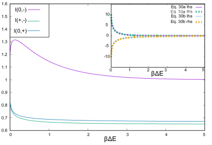
Figure 1: $I(k,l)$ as function of the normalized inverse temperature $\beta\Delta E$. DBE only holds if all the $I(k,l)=1$. For large $\beta\Delta E$, $I(0,-)$ tends to 1. Nevertheless, $I(+,-)$ and $I(0,+)$ are still different from 1 indicating the lack of DBE. Inset: Left hand side, lhs, (continuous line) and right hand side, rhs (dotted line), of the thermalization conditions, Eqs. 30a and 30b. The compliance with these conditions (lhs=rhs) verifies our numeric calculation. The y-axis of the inset has been multiplied by a factor of $10^{4}$. Parameters: ${\cal V}_{1}=1$,${\cal V}_{2}=0.7$, ${\cal V}_{3}=1.5$, $\mathcal{E}_{+}=0.5$, $\mathcal{E}_{0}=0.0$, $\mathcal{E}_{-}=-0.5$ and $\Delta E=\mathcal{E}_{0}-\mathcal{E}_{-}$. For more details see SI.

DBE establishes a relation between transition rates involving the same Bohr frequencies (i.e., $a_{kl}$ and $a_{lk}$) allowing independent transition rates among different Bohr frequency [16]. This relation, together with the Kubo-Martin-Schwinger condition (KMS), forces the reduced system to thermalize. In contrast, systems violating DBE use a different thermalization mechanism. While they have some extra degree of freedom due to the DBE violation, thermalization imposes a complex dependence among rates for different Bohr frequencies that we term thermalization conditions. For example, in the case of the 3QD model they read

$$a_{+0}\left[1-I(0,+)\right]=a_{-0}\left[I(0,-)-1\right];$$ (30a)

$$a_{0+}\left[1-1/I(0,+)\right]=a_{-+}\left[I(+,-)-1\right].$$ (30b)

V.1 Probabillity and heat currents

The different thermalization mechanisms could be better understood by analyzing the probability currents, $K_{jk}$ (see discussion below Eq. (26) and Ref.[4]). Systems complying with DBE thermalize by reducing each individual probability’s currents, until all of them become zero at thermal equilibrium. In contrast, systems violating DBE thermalize by reducing $\sum_{j}K_{jk}$ which becomes zero at thermal equilibrium, while at least some of the individual currents,

$$K_{jk}=a_{kj}p^{eq}_{k}\left[I(j,k)-1\right],$$ (31)

remain nonzero even at equilibrium forming closed loops. These persistent currents are different from those found on aromatic [54, 55, 56] or mesoscopic rings [57, 58]. The currents found in these works are also present in isolated systems. They are produced by breaking the time-reversal symmetry of the system eigenfunctions [59]. In contrast, the current described by Eq. (31) requires a nonisolated system and the breakdown of other symmetries (see section III).

It has been claimed that violation of DBE produces persistent heat currents in nonreciprocal systems [29]. The existence of these currents does not violate any fundamental thermodynamic law. Using the Spohn inequality it is possible to define thermodynamically consistent heat currents [60] between individual pairs of the system energy levels and the thermal bath. At the equilibrium state they are defined as $J_{ml}=-\beta^{-1}{a_{lm}p^{eq}_{m}}\left[I(m,l)-1\right]\ln\left(p_{m}^{eq}/p_{l}^{eq}\right)$. In particular for the toy model we get ($i,j=0,+,-$)

$$J_{ij}=N\left[I(+,-)-1\right](\mathcal{E}_{i}-\mathcal{E}_{j}),$$ (32)

where $N=a_{-+}e^{-\beta(\mathcal{E}_{-}-\mathcal{E}_{0})}[1+e^{-\beta(\mathcal{E}_{-}-\mathcal{E}_{0})}+e^{-\beta(\mathcal{E}_{+}-\mathcal{E}_{0})}]^{-1}$. Even though there are heat currents to and from individual pairs of the system energy levels, the total heat exchange between the bath and the system is zero, as expected from the first law of thermodynamics. It is important to notice that both probabilities and heat currents are related to transitions between delocalized energy levels and do not necessarily imply the existence of heat currents in space. In particular, for our 3QD model all energy eigenstates yield equal occupation probabilities for all dots.

In summary, here we develop an open quantum system framework to study systems that violate DBE. This extra degree of freedom changes the system dynamics and could be beneficial for many applications, such as: speeding up thermalization, increasing the sensitivity of measuring devices, and improving the operation of heat machines. One should stress that DBE is not easy to break. The effect appears in the higher-order expansion with respect to the system-bath coupling constant and could vanish in the presence of certain spatial symmetries (see SI).

Acknowledgement We thank Natan Granit, Thales Pinto Silva, U. Peskin and N. Moiseyev for useful discussions. R. A. is supported by the Foundation for Polish Science’s International Research Agendas, with structural funds from the European Union (EU) for the ICTQT and at the Technion by a fellowship from the Lady Davis Foundation. M. Š. gratefully acknowledges financial support of the Helen Diller Quantum Center of the Technion (March 1 - May 31, 2023). D.G.K. is supported by the ISRAEL SCIENCE FOUNDATION (grant No. 2247/22) and by the Council for Higher Education Support Program for Hiring Outstanding Faculty Members in Quantum Science and Technology in Research Universities.

Violation of Detailed Balance in Quantum Open Systems: Supplementary information

The purpose of this supplementary information is to introduce a simple toy model which is used in the main text to explicitly illustrate the violation of detailed balance. We start with a rather general setup and go subsequently into a more specific setting which enables us to obtain $I(k,l)$ semianalytically without any approximations.

S1 General setup for the toy model

We consider a non-relativistic quantum particle in a $d$-dimensional space. The corresponding Hilbert space is spanned by the momentum basis $|{\bm{p}}\rangle$, or equivalently by the position basis $|{\bm{q}}\rangle$. For a joined system-particle basis one has

$$\langle{\bm{q}}\,j|{\bm{p}}\,j^{\prime}\rangle\;=\;\delta_{jj^{\prime}}\,\frac{e^{\frac{i}{\hbar}{\bm{p}}\bm{\cdot}{\bm{q}}}}{(2\,\pi\,\hbar)^{d/2}}.$$ (S1)

State vectors $|\Psi\rangle$ can be represented by wavefunctions

$$\Psi_{j}({\bm{q}})\;=\;\langle{\bm{q}}\,j|\Psi\rangle,\hskip 14.22636pt\tilde{\Psi}_{j}({\bm{p}})\;=\;\langle{\bm{p}}\,j|\Psi\rangle.$$ (S2)

The Hamiltonian $H_{0}=H_{S}+H_{P}$ of our two isolated subsystems satisfies

$$H_{0}\,|{\bm{p}}\,j\rangle\;=\;\Bigl{(}E_{p}+{\cal E}_{j}\Bigr{)}\,|{\bm{p}}\,j\rangle;$$ (S3)

here $E_{p}=\frac{p^{2}}{2\,m}$. The interaction among the two subsystems, $H_{int}$ is defined by prescription

$$\langle{\bm{p}}\,j|H_{int}|\Psi\rangle\;=\;\Theta(P-p)\,\sum_{j^{\prime}}\sum_{\iota}\,v_{jj^{\prime}}^{\iota,P}\,\Psi_{j^{\prime}}({\bm{q}}_{\iota})\;\frac{e^{-\frac{i}{\hbar}{\bm{p}}\bm{\cdot}{\bm{q}}_{\iota}}}{(2\,\pi\,\hbar)^{d/2}};$$ (S4)

here $P$ is the momentum UV cutoff needed for eventual renormalization. One may ask at this point where the particular form (S4) of the coupling comes from.
Here is the answer:

$$\langle{\bm{p}}\,j|\left(\sum_{\iota}\,|\chi_{\iota}\rangle\,{\cal V}_{\iota}\;\delta^{d}(\hat{\bm{q}}-{\bm{q}}_{\iota})\;\langle\chi_{\iota}|\right)\int_{{\mathbb{R}}^{d}}{\rm d}^{d}q^{\prime}\sum_{j^{\prime}}\Psi_{j^{\prime}}({\bm{q}}^{\prime})\;|{\bm{q}}^{\prime}\,j^{\prime}\rangle\;=$$ (S5)

$$= \sum_{j^{\prime}}\sum_{\iota}\,\Bigl{(}\,\langle j|\chi_{\iota}\rangle\,{\cal V}_{\iota}\,\langle\chi_{\iota}|j^{\prime}\rangle\Bigr{)}\,_{\rm el}\langle{\bm{p}}|{\bm{q}}_{\iota}\rangle_{\rm el}\,\Psi_{j^{\prime}}({\bm{q}}_{\iota}).$$

Let us look now at the implicit Lippmann-Schwinger equation (LSE)

$$|\Psi\rangle\;=\;|{\bm{p}}\,j\rangle\;+\;G_{0}\,H_{int}\,|\Psi\rangle.$$ (S6)

Here $G_{0}$ is the free Green’s operator, $G_{0}=\frac{1}{E_{p}+{\cal E}_{j}-H_{0}+i\varepsilon}$. The corresponding $T$-matrix elements are given simply as

$$\langle{\bm{p}}^{\prime}\,j^{\prime}|\,T\,|{\bm{p}}\,j\rangle\;=\;\langle{\bm{p}}^{\prime}\,j^{\prime}|\,H_{int}\,|\Psi\rangle=\langle{\bm{p}}^{\prime}\,j^{\prime}|H_{int}|{\bm{p}}\,j\rangle+\langle{\bm{p}}^{\prime}\,j^{\prime}|H_{int}G_{0}H_{int}|\Psi\rangle.$$ (S7)

Moreover, we can rewrite the above two expressions in terms of the full Green’s operator, $G=\frac{1}{E_{p}+{\cal E}_{j}-H_{tot}+i\varepsilon}$. One has

$$|\Psi\rangle\;=\;|{\bm{p}}\,j\rangle\;+\;G\,H_{int}\,|{\bm{p}}\,j\rangle\;;$$ (S8)

and

$$\langle{\bm{p}}^{\prime}\,j^{\prime}|\,T\,|{\bm{p}}\,j\rangle\;=\langle{\bm{p}}^{\prime}\,j^{\prime}|H_{int}|{\bm{p}}\,j\rangle+\langle{\bm{p}}^{\prime}\,j^{\prime}|H_{int}GH_{int}|{\bm{p}}\,j\rangle\;.$$ (S9)

Equation (S9) can be used to relate the $T-$matrix properties with the full Green’s operator and, in this way, determine the necessary conditions on the full Green’s operator for DBE. For example, if $\langle{\bm{p}}^{\prime}j^{\prime}|H_{int}|{\bm{p}}j\rangle$ is a symmetric matrix, then the same applies also for the matrix elements of $G$, and therefore also the $T$-matrix elements are symmetric. Establishing the requirement on the Green’s function for complying with the other conditions on the $T$-matrix (hermiticity, time reversal with and without parity, see section III on the main text) is left for future works.

Let us return now to equation (S7). The r.h.s. can actually be evaluated explicitly as above in (S4). Meaning also that all the $T$-matrix elements are completely specified by knowledge of $\{\Psi_{j}({\bm{q}}_{\iota})\}_{j,\iota}$. Note also that

$$\langle{\bm{p}}^{\prime}\,j^{\prime}|\,\frac{1}{E_{p}+{\cal E}_{j}-H_{0}+i\varepsilon}\,|{\bm{p}}^{\prime\prime}\,j^{\prime\prime}\rangle\;=\;\frac{\delta^{d}({\bm{p}}^{\prime}-{\bm{p}}^{\prime\prime})\;\delta_{j^{\prime}j^{\prime\prime}}}{E_{p}+{\cal E}_{j}-E_{p^{\prime}}-{\cal E}_{j^{\prime}}+i\varepsilon}.$$ (S10)

Returning to (S6) and taking advantage of (S10) and (S4). One gets

$$\tilde{\Psi}_{j^{\prime}}({\bm{p}}^{\prime}) = \delta^{d}({\bm{p}}-{\bm{p}}^{\prime})\;\delta_{jj^{\prime}}\;+\;\int_{{\mathbb{R}}^{d}}{\rm d}^{d}p^{\prime\prime}\sum_{j^{\prime\prime}}\,\frac{\delta^{d}({\bm{p}}^{\prime}-{\bm{p}}^{\prime\prime})\;\delta_{j^{\prime}j^{\prime\prime}}}{E_{p}+{\cal E}_{j}-E_{p^{\prime}}-{\cal E}_{j^{\prime}}+i\varepsilon}\;\langle{\bm{p}}^{\prime\prime}\,j^{\prime\prime}|H_{int}|\Psi\rangle\;=$$ (S11)

$$= \delta^{d}({\bm{p}}-{\bm{p}}^{\prime})\;\delta_{jj^{\prime}}\;+\;\frac{\langle{\bm{p}}^{\prime}\,j^{\prime}|H_{int}|\Psi\rangle}{E_{p}+{\cal E}_{j}-E_{p^{\prime}}-{\cal E}_{j^{\prime}}+i\varepsilon}\;=$$

$$= \delta^{d}({\bm{p}}-{\bm{p}}^{\prime})\;\delta_{jj^{\prime}}\;+\;\frac{\Theta(P-p^{\prime})}{E_{p}+{\cal E}_{j}-E_{p^{\prime}}-{\cal E}_{j^{\prime}}+i\varepsilon}\;\sum_{j^{\prime\prime}}\sum_{\iota}\,v_{j^{\prime}j^{\prime\prime}}^{\iota,P}\,\Psi_{j^{\prime\prime}}({\bm{q}}_{\iota})\;\frac{e^{-\frac{i}{\hbar}{\bm{p}}^{\prime}\bm{\cdot}{\bm{q}}_{\iota}}}{(2\,\pi\,\hbar)^{d/2}}.$$

Showing once again that the scattering wavefunction $\tilde{\Psi}_{j^{\prime}}({\bm{p}}^{\prime})$ is known iff a finite sequence of values of $\{\Psi_{j^{\prime\prime}}({\bm{q}}_{\iota})\}_{j^{\prime\prime}\iota}$ is known. In passing we note that there is no scattering for $p^{\prime}>P$ due to presence of $\Theta(P-p^{\prime})$. What remains to be done is to find the above mentioned values of $\{\Psi_{j}({\bm{q}}_{\iota})\}_{j,\iota}$.
One has

$$\Psi_{j^{\prime}}({\bm{q}}_{\iota^{\prime}})\;=\;\int_{{\mathbb{R}}^{d}}{\rm d}^{d}p^{\prime}\;\tilde{\Psi}_{j^{\prime}}({\bm{p}}^{\prime})\;\frac{e^{+\frac{i}{\hbar}{\bm{p}}^{\prime}\bm{\cdot}{\bm{q}}_{\iota^{\prime}}}}{(2\,\pi\,\hbar)^{d/2}};$$ (S12)

and (S11) provides immediately

$$\Psi_{j^{\prime}}({\bm{q}}_{\iota^{\prime}})=\frac{e^{+\frac{i}{\hbar}{\bm{p}}\bm{\cdot}{\bm{q}}_{\iota^{\prime}}}}{(2\,\pi\,\hbar)^{d/2}}\;\delta_{jj^{\prime}}+\sum_{j^{\prime\prime}}\sum_{\iota^{\prime\prime}}\,\left\{\,\frac{v_{j^{\prime}j^{\prime\prime}}^{\iota^{\prime\prime},P}}{(2\,\pi\,\hbar)^{d}}\int_{{\mathbb{R}}^{d}}{\rm d}^{d}p^{\prime}\;\frac{\Theta(P-p^{\prime})\;e^{+\frac{i}{\hbar}{\bm{p}}^{\prime}\bm{\cdot}({\bm{q}}_{\iota^{\prime}}-{\bm{q}}_{\iota^{\prime\prime}})}}{E_{p}+{\cal E}_{j}-E_{p^{\prime}}-{\cal E}_{j^{\prime}}+i\varepsilon}\,\right\}\Psi_{j^{\prime\prime}}({\bm{q}}_{\iota^{\prime\prime}}).$$ (S13)

The just obtained outcome (S13) represents a set of linear inhomogeneous equations for the unknowns $\{\Psi_{j}({\bm{q}}_{\iota})\}_{j,\iota}$. It can be solved either analytically or numerically, assuming tacitly regularity. Having the coefficients $\{\Psi_{j}({\bm{q}}_{\iota})\}_{j,\iota}$ in hand, all the $T$-matrix elements (S7) can be accessed using (S4). Such that

$$\langle{\bm{p}}^{\prime}\,j^{\prime}|\,T\,|{\bm{p}}\,j\rangle\;=\;\Theta(P-p^{\prime})\,\sum_{j^{\prime\prime}}\sum_{\iota^{\prime\prime}}\,v_{j^{\prime}j^{\prime\prime}}^{\iota^{\prime\prime},P}\,\Psi_{j^{\prime\prime}}({\bm{q}}_{\iota^{\prime\prime}})\;\frac{e^{-\frac{i}{\hbar}{\bm{p}}^{\prime}\bm{\cdot}{\bm{q}}_{\iota^{\prime\prime}}}}{(2\,\pi\,\hbar)^{d/2}}.$$ (S14)

The final outcome of our above pursued analysis can be summarized by working equations (S13) and (S14).

S1.a Short separation

Substantial simplification follows when all the sites ${\bm{q}}_{\iota}$ are placed at the origin ${\bm{0}}$.
One has

$$\Psi_{j^{\prime}}=\frac{\delta_{jj^{\prime}}}{(2\,\pi\,\hbar)^{d/2}}+\frac{1}{(2\,\pi\,\hbar)^{d}}\,\int_{{\mathbb{R}}^{d}}{\rm d}^{d}p^{\prime}\;\frac{\Theta(P-p^{\prime})}{E_{p}+{\cal E}_{j}-E_{p^{\prime}}-{\cal E}_{j^{\prime}}+i\varepsilon}\;\sum_{j^{\prime\prime}}v_{j^{\prime}j^{\prime\prime}}^{P}\;\Psi_{j^{\prime\prime}};$$ (S15)

with

$$v_{j^{\prime}j^{\prime\prime}}^{P}\;=\;\sum_{\iota^{\prime\prime}}\,v_{j^{\prime}j^{\prime\prime}}^{\iota^{\prime\prime},P};$$ (S16)

and $\Psi_{j^{\prime}}\equiv\Psi_{j^{\prime}}({\bm{0}})$. Equation (S14) for the $T$-matrix elements boils down into

$$\langle{\bm{p}}^{\prime}\,j^{\prime}|\,T\,|{\bm{p}}\,j\rangle\;=\;\frac{\Theta(P-p^{\prime})}{(2\,\pi\,\hbar)^{d/2}}\,\sum_{j^{\prime\prime}}\,v_{j^{\prime}j^{\prime\prime}}^{P}\,\Psi_{j^{\prime\prime}}.$$ (S17)

Combining (S17) and (S15) yields an even simpler formula

$$\langle{\bm{p}}^{\prime}\,j^{\prime}|\,T\,|{\bm{p}}\,j\rangle\;=\;\Theta(P-p^{\prime})\,\left(\,\int_{{\mathbb{R}}^{d}}{\rm d}^{d}p^{\prime\prime}\;\frac{\Theta(P-p^{\prime\prime})}{E_{p}+{\cal E}_{j}-E_{p^{\prime\prime}}-{\cal E}_{j^{\prime}}+i\varepsilon}\,\right)^{-1}\Bigl{(}(2\,\pi\,\hbar)^{d/2}\,\Psi_{j^{\prime}}\,-\,\delta_{jj^{\prime}}\Bigr{)}.$$ (S18)

The final outcome of the just presented analysis can be summarized by equations (S15) and (S18). Note that the $T$-matrix elements coming out of (S18) are, by construction, independent upon the directions of ${\bm{p}}$ and ${\bm{p}}^{\prime}$.

S1.b One dimensional case

The UV cutoff $P$ can be lifted to $+\infty$, since for $d=1$ no renormalization is needed. Contour integration (residue theorem) provides the required integral

$$\int_{-\infty}^{+\infty}{\rm d}p^{\prime}\;\frac{1}{E_{p}+{\cal E}_{j}-E_{p^{\prime}}-{\cal E}_{j^{\prime}}+i\varepsilon}\;=\;-\,i\,\pi\,\sqrt{\frac{2\,m}{E-{\cal E}_{j^{\prime}}}};$$ (S19)

here $E=E_{p}+{\cal E}_{j}$. Note that $E-{\cal E}_{j^{\prime}}>0$ as long as the $j^{\prime}$-th channel is open for scattering, and $E-{\cal E}_{j^{\prime}}<0$ as long as the $j^{\prime}$-th channel is closed for scattering. For the sake of clarity, we present explicitly the calculation leading to (S19):

$$\int_{-\infty}^{+\infty}\frac{{\rm d}p^{\prime}}{E-{\cal E}_{j^{\prime}}+i\varepsilon-E_{p^{\prime}}}\;=2\,m\,\int_{-\infty}^{+\infty}\frac{{\rm d}p^{\prime}}{2\,m\,(E-{\cal E}_{j^{\prime}}+i\varepsilon)-p^{\prime 2}}\;=-\,2\,m\,\int_{-\infty}^{+\infty}\frac{{\rm d}p^{\prime}}{(p^{\prime}-y)(p^{\prime}+y)};$$ (S20)

where

$$y\;=\;\sqrt{2\,m\,(E-{\cal E}_{j^{\prime}}+i\varepsilon)},\hskip 14.22636pt\hbox{Re}~{}\,y>0,\hskip 14.22636pt\hbox{Im}~{}\,y>0.$$ (S21)

The integration contour over $p^{\prime}$ can now be closed in the upper half of the complex $p^{\prime}$-plane. In this way only the pole $p^{\prime}=y$ is encircled, and the residue theorem yields accordingly

$$\int_{-\infty}^{+\infty}\frac{{\rm d}p^{\prime}}{E-{\cal E}_{j^{\prime}}+i\varepsilon-E_{p^{\prime}}}\;=\;-\,i\,\pi\,\sqrt{\frac{2\,m}{E-{\cal E}_{j^{\prime}}+i\varepsilon}}.$$ (S22)

Thereby (S19) is obtained for $\varepsilon\to+0$. Equation (S15) boils down into

$$\Psi_{j^{\prime}} = \frac{\delta_{jj^{\prime}}}{\sqrt{2\,\pi\,\hbar}}\;-\;\frac{i}{2\,\hbar}\,\sqrt{\frac{2\,m}{E-{\cal E}_{j^{\prime}}}}\;\sum_{j^{\prime\prime}}v_{j^{\prime}j^{\prime\prime}}\;\Psi_{j^{\prime\prime}}.$$ (S23)

Equation (S18) boils down into

$$\langle p^{\prime}\,j^{\prime}|\,T\,|p\,j\rangle\;=\;\frac{i}{\pi}\;\sqrt{\frac{E-{\cal E}_{j^{\prime}}}{2\,m}}\,\Bigl{(}\sqrt{2\,\pi\,\hbar}\,\Psi_{j^{\prime}}\,-\,\delta_{jj^{\prime}}\Bigr{)}.$$ (S24)

S2 Three levels system toy model

In particular, we consider the three-level system described in the main text. Its Hamiltonian is defined in the main text Eq. 28. The localized basis, ($|1\rangle$, $|2\rangle$ and $|3\rangle$) corresponds to the states $|\chi_{\iota}\rangle$ in Eq. S5 of this supplement and $|j\rangle$, with $(j=-1,0,+1)$, to the three-level system eigenstates. Using the relation between the localized basis and the system Hamiltonian [3], one can find $v_{j^{\prime}j^{\prime\prime}}$:

$$v_{jj}=\frac{\mathcal{V}_{1}+\mathcal{V}_{2}+\mathcal{V}_{3}}{3};$$ (S25)

$$v_{0+}=v_{+-}=v_{-0}=\frac{1}{3}\left(\mathcal{V}_{1}+\mathcal{V}_{2}e^{i2\pi/3}+\mathcal{V}_{3}e^{-i2\pi/3}\right)=\frac{1}{3}\left(\mathcal{V}_{1}-\frac{1}{2}(\mathcal{V}_{2}+\mathcal{V}_{3})+i\frac{\sqrt{3}}{2}(\mathcal{V}_{2}-\mathcal{V}_{3})\right);$$ (S26)

$$v_{0-}=v_{-+}=v_{+0}=\frac{1}{3}\left(\mathcal{V}_{1}+\mathcal{V}_{2}e^{-i2\pi/3}+\mathcal{V}_{3}e^{i2\pi/3}\right)=\frac{1}{3}\left(\mathcal{V}_{1}-\frac{1}{2}(\mathcal{V}_{2}+\mathcal{V}_{3})-i\frac{\sqrt{3}}{2}(\mathcal{V}_{2}-\mathcal{V}_{3})\right).$$ (S27)

Assuming $j=0$, and replacing the coefficients above into Eq. S23 we get:

$$\Psi_{0}=\frac{1}{\sqrt{2\pi\hbar}}-\frac{i}{2\hbar}\sqrt{\frac{2m}{E-\mathcal{E}_{0}}}\left(v_{0,0}\Psi_{0}+v_{0,+}\Psi_{+}+v_{0,-}\Psi_{-}\right),$$ (S28)

$$\Psi_{+}=-\frac{i}{2\hbar}\sqrt{\frac{2m}{E-\mathcal{E}_{+}}}\left(v_{+,0}\Psi_{0}+v_{+,+}\Psi_{+}+v_{+,-}\Psi_{-}\right),$$ (S29)

$$\Psi_{-}=-\frac{i}{2\hbar}\sqrt{\frac{2m}{E-\mathcal{E}_{-}}}\left(v_{-,0}\Psi_{0}+v_{-,+}\Psi_{+}+v_{-,-}\Psi_{-}\right),$$ (S30)

Solving the equations above and using (S25),(S26) and (S27), we get:

$$\Psi_{0}=N_{\Psi}\left[(-i(-i+b_{-}v_{0,0})(-i+b_{+}v_{0,0})+ib_{-}b_{+}v_{-,0}v_{+,0})\right],$$ (S31)

$$\Psi_{+}=N_{\Psi}\left[b_{+}(v_{+,0}-ib_{-}(v_{-,0}^{2}-v_{0,0}v_{+,0})))\right],$$ (S32)

$$\Psi_{-}=N_{\Psi}\left[b_{-}(v_{-,0}-ib_{+}(v_{+,0}^{2}-v_{0,0}v_{-,0}))\right],$$ (S33)

where $b_{i}=\frac{1}{2\hbar}\sqrt{\frac{2m}{E-\mathcal{E}_{i}}}$ and

$$\frac{1}{N_{\Psi}}=-i(-i+b_{-}v_{0,0})(-i+b_{+}v_{0,0})+ib_{-}b_{+}v_{-,0}v_{+,0}+$$

$$b_{0}\left(-i(b_{-}+b_{+})v_{0,0}^{2}+b_{-}b_{+}v_{0,0}^{3}+b_{-}b_{+}v_{-,0}^{3}+i(b_{-}+b_{+})v_{-,0}v_{+,0}+b_{-}b_{+}v_{+,0}^{3}-v_{0,0}(1+3b_{-}b_{+}v_{-,0}v_{+,0})\right).$$ (S34)

In a similar way, the scattering wavefunctions can be deduced for $j=+$ and $j=-$. Having the scattering wavefunctions it is straigthforward to obtain the $T$-Matrix elements using Eq. S24 of this supplement.

S2.a Detailed balance conditions on the T-matrix for a toy model

In this section we show that our toy model breaks the four detailed balance conditions (see Section III on the main text). In particular we will show that the necessary conditions for $I(+,0)\neq 1$ are met. For our toy model:

$$\langle p^{\prime}+|T|p\,0\rangle=\frac{iN_{\Psi}}{\sqrt{2\pi\hbar}}(v_{+,0}-ib_{-}(v_{-,0}^{2}-v_{0,0}v_{+,0})),$$ (S35)

$$\langle p\,0|T|p^{\prime}+\rangle=\frac{iN_{\Psi}}{\sqrt{2\pi\hbar}}(v_{-,0}-ib_{-}(v_{+,0}^{2}-v_{0,0}v_{-,0})).$$ (S36)

Here the normalization prefactor is given by

$$\frac{1}{N_{\Psi}}=$$

$$i+b_{0}b_{-}b_{+}\mathcal{V}_{1}\mathcal{V}_{2}\mathcal{V}_{3}+\frac{1}{3}(b_{0}+b_{-}+b_{+})\left(\mathcal{V}_{1}+\mathcal{V}_{2}+\mathcal{V}_{3}\right)-\frac{i}{3}\left(b_{-}b_{+}+b_{0}(b_{-}+b_{+})\right)\left(\mathcal{V}_{1}\mathcal{V}_{2}+\mathcal{V}_{1}\mathcal{V}_{3}+\mathcal{V}_{2}\mathcal{V}_{3}\right).$$ (S37)

Besides the resonances, $E=\mathcal{E}_{j}$, $N_{\Psi}$ is a finite number for finite potentials. This implies that $N_{\Psi}$ in general is nonzero.

Hermiticity

In order to check hermiticity we do a series expansion on the coupling strength, $v_{ij}$. Hermiticity is broken at second order, as shown below:

$$\langle p^{\prime}+|T|p\,0\rangle-\langle p\,0|T|p^{\prime}+\rangle^{*}=\frac{-i}{\sqrt{2\pi\hbar}}\left(2Re\left(b_{-}\right)v_{-0}^{2}+2v_{+0}v_{00}\left(Re(b_{+})+Re(b_{0})\right)\right)+O(v^{3}_{ij}),$$ (S38)

which besides some very specific values of $E$ is different from zero as long as not all the potentials are the same.

Symmetric matrix

$$\langle p^{\prime}+|T|p\,0\rangle-\langle p\,0|T|p^{\prime}+\rangle=\frac{N_{\Psi}(\mathcal{V}_{2}-\mathcal{V}_{3})}{\sqrt{6\pi\hbar}}\left(1+ib_{-}\mathcal{V}_{1}\right),$$ (S39)

which is different from zero as long as $\mathcal{V}_{2}\neq\mathcal{V}_{3}$. This expression is correct for any coupling strength.

Time reversal symmetry with and without parity transformation:

In our toy model the T-matrix is invariant under parity transformation. Therefore, these two conditions are actually the same and here we just prove the time reversal symmetry with parity transformation.

$$|\langle p^{\prime}+|T|p\,0\rangle|^{2}-|\langle p\,0|T|p^{\prime}+\rangle|^{2}=\frac{|N_{\Psi}|^{2}Re(b_{-})}{3\sqrt{3}\pi\hbar}(\mathcal{V}_{1}-\mathcal{V}_{3})(\mathcal{V}_{2}-\mathcal{V}_{3})(\mathcal{V}_{1}-\mathcal{V}_{3}),$$ (S40)

which is different from zero as long as all the potentials are different. This expression is correct for any coupling strength.

S2.b Calculating $I(k,l)$ for a toy model

Despite breaking all the sufficient conditions on the T-matrix for DBE, there could be cases where DBE is still preserved. To confirm that DBE is actually broken, we explicitly calculate $I(k,l)$. For this, we numerically compute the following integrals:

$$A_{\beta}(j^{\prime},j) = \int_{-\infty}^{+\infty}{\rm d}p\int_{-\infty}^{+\infty}{\rm d}p^{\prime}\;\,e^{-\beta E_{p}}\;\delta\Bigl{(}E_{p}\,+\,{\cal E}_{j}\,-\,E_{p^{\prime}}\,-\,{\cal E}_{j^{\prime}}\Bigr{)}\;\Bigl{|}\,\langle p^{\prime}\,j^{\prime}|\,T\,|p\,j\rangle\,\Bigr{|}^{2}\;=$$ (S41)

$$= 2\,m\,\int_{{\cal E}_{j}}^{\infty}{\rm d}E\;\,\frac{e^{-\beta(E-{\cal E}_{j})}}{\sqrt{(E-{\cal E}_{j})(E-{\cal E}_{j^{\prime}})}}\;\Bigl{|}\,\langle p^{\prime}\,j^{\prime}|\,T\,|p\,j\rangle\,\Bigr{|}^{2};$$

and

$$B_{\beta}(j^{\prime},j) = \int_{-\infty}^{+\infty}{\rm d}p\int_{-\infty}^{+\infty}{\rm d}p^{\prime}\;\,e^{-\beta E_{p}}\;\delta\Bigl{(}E_{p}\,+\,{\cal E}_{j}\,-\,E_{p^{\prime}}\,-\,{\cal E}_{j^{\prime}}\Bigr{)}\;\Bigl{|}\,\langle p\,j|\,T\,|p^{\prime}\,j^{\prime}\rangle\,\Bigr{|}^{2}\;=$$ (S42)

$$= 2\,m\,\int_{{\cal E}_{j}}^{\infty}{\rm d}E\;\,\frac{e^{-\beta(E-{\cal E}_{j})}}{\sqrt{(E-{\cal E}_{j})(E-{\cal E}_{j^{\prime}})}}\;\Bigl{|}\,\langle p\,j|\,T\,|p^{\prime}\,j^{\prime}\rangle\,\Bigr{|}^{2}.$$

Subsequently, we also get the ratio

$$I_{\beta}(j^{\prime},j)\;=\;\frac{A_{\beta}(j^{\prime},j)}{B_{\beta}(j^{\prime},j)}.$$ (S43)

Having in hand $I_{\beta}(j^{\prime},j)$, we can even check the validity of the two thermalization conditions (Eqs. 30a and 30b in the main text). The obtained numerical results are presented graphically in the main text.

References

• Lewis [1925] G. N. Lewis, A new principle of equilibrium, Proceedings of the National Academy of Sciences of the United States of America 11, 179 (1925).
• Fowler and Milne [1925] R. H. Fowler and E. A. Milne, A note on the principle of detailed balancing, Proceedings of the National Academy of Sciences of the United States of America 11, 400 (1925).
• Spohn [1978] H. Spohn, Entropy production for quantum dynamical semigroups, Journal of Mathematical Physics 19, 1227 (1978).
• Zia and Schmittmann [2007] R. K. P. Zia and B. Schmittmann, Probability currents as principal characteristics in the statistical mechanics of non-equilibrium steady states, Journal of Statistical Mechanics: Theory and Experiment 2007, P07012 (2007).
• Onsager [1931a] L. Onsager, Reciprocal relations in irreversible processes. I, Physical Review 37, 405 (1931a).
• Onsager [1931b] L. Onsager, Reciprocal relations in irreversible processes. II, Physical Review 38, 2265 (1931b).
• Boyd [1977] R. K. Boyd, Macroscopic and microscopic restrictions on chemical kinetics, Chemical Reviews 77, 93 (1977).
• Kubo [1966] R. Kubo, The fluctuation-dissipation theorem, Reports on Progress in Physics 29, 255 (1966).
• Cengio et al. [2021] S. D. Cengio, D. Levis, and I. Pagonabarraga, Fluctuation-Dissipation Relations in the absence of Detailed Balance: formalism and applications to Active Matter, Journal of Statistical Mechanics: Theory and Experiment 2021, 043201 (2021).
• Crooks [1999] G. E. Crooks, Entropy production fluctuation theorem and the nonequilibrium work relation for free energy differences, Physical Review E 60, 2721 (1999).
• Crooks [1998] G. E. Crooks, Nonequilibrium measurements of free energy differences for microscopically reversible Markovian systems, Journal of Statistical Physics 90, 1481 (1998).
• Kurchan [1998] J. Kurchan, Fluctuation theorem for stochastic dynamics, Journal of Physics A: Mathematical and General 31, 3719 (1998).
• Kossakowski et al. [1977] A. Kossakowski, A. Frigerio, V. Gorini, and M. Verri, Quantum detailed balance and KMS condition, Communications in Mathematical Physics 57, 97 (1977).
• Alicki [1976] R. Alicki, On the detailed balance condition for non-Hamiltonian systems, Reports on Mathematical Physics 10, 249 (1976), iSBN: 0034-4877 Publisher: Elsevier.
• Snyder et al. [1998] W. C. Snyder, Z. Wan, and X. Li, Thermodynamic constraints on reflectance reciprocity and Kirchhoff’s law, Applied Optics 37, 3464 (1998).
• Dann and Kosloff [2021] R. Dann and R. Kosloff, Open system dynamics from thermodynamic compatibility, Physical Review Research 3, 023006 (2021), publisher: APS.
• Battle et al. [2016] C. Battle, C. P. Broedersz, N. Fakhri, V. F. Geyer, J. Howard, C. F. Schmidt, and F. C. MacKintosh, Broken detailed balance at mesoscopic scales in active biological systems, Science 352, 604 (2016).
• Gnesotto et al. [2018] F. S. Gnesotto, F. Mura, J. Gladrow, and C. P. Broedersz, Broken detailed balance and non-equilibrium dynamics in living systems: a review, Reports on Progress in Physics 81, 066601 (2018).
• Platini [2011] T. Platini, Measure of the violation of the detailed balance criterion: A possible definition of a “distance” from equilibrium, Physical Review E 83, 011119 (2011).
• Thomsen [1953] J. S. Thomsen, Logical relations among the principles of statistical mechanics and thermodynamics, Physical Review 91, 1263 (1953).
• Johnson and Goody [2011] K. A. Johnson and R. S. Goody, The original Michaelis constant: translation of the 1913 Michaelis–Menten paper, Biochemistry 50, 8264 (2011).
• Voorsluijs et al. [2020] V. Voorsluijs, F. Avanzini, and M. Esposito, Thermodynamic validity criterion for the irreversible Michaelis-Menten equation, arXiv preprint arXiv:.06476  (2020).
• MacDonald et al. [1968] C. T. MacDonald, J. H. Gibbs, and A. C. Pipkin, Kinetics of biopolymerization on nucleic acid templates, Biopolymers: Original Research on Biomolecules 6, 1 (1968).
• Derrida et al. [1993] B. Derrida, S. A. Janowsky, J. L. Lebowitz, and E. R. Speer, Exact solution of the totally asymmetric simple exclusion process: shock profiles, Journal of Statistical Physics 73, 813 (1993).
• Hinrichsen [2000] H. Hinrichsen, Non-equilibrium critical phenomena and phase transitions into absorbing states, Advances in Physics 49, 815 (2000).
• Caloz et al. [2018] C. Caloz, A. Alù, S. Tretyakov, D. Sounas, K. Achouri, and Z.-L. Deck-Léger, Electromagnetic nonreciprocity, Physical Review Applied 10, 047001 (2018).
• Asadchy et al. [2020] V. S. Asadchy, M. S. Mirmoosa, A. Diaz-Rubio, S. Fan, and S. A. Tretyakov, Tutorial on electromagnetic nonreciprocity and its origins, Proceedings of the IEEE 108, 1684 (2020).
• Zhu and Fan [2014] L. Zhu and S. Fan, Near-complete violation of detailed balance in thermal radiation, Physical Review B 90, 220301 (2014).
• Zhu and Fan [2016] L. Zhu and S. Fan, Persistent directional current at equilibrium in nonreciprocal many-body near field electromagnetic heat transfer, Physical Review Letters 117, 134303 (2016).
• Gelbwaser-Klimovsky et al. [2022] D. Gelbwaser-Klimovsky, N. Graham, M. Kardar, and M. Krüger, Equilibrium forces on nonreciprocal materials, Physical Review B 106, 115106 (2022), publisher: American Physical Society.
• Herz and Biehs [2019] F. Herz and S. A. Biehs, Green-Kubo relation for thermal radiation in non-reciprocal systems, EPL 127, 44001 (2019).
• Ben-Abdallah [2016] P. Ben-Abdallah, Photon thermal hall effect, Physical Review Letters 116, 084301 (2016).
• Latella and Ben-Abdallah [2017] I. Latella and P. Ben-Abdallah, Giant thermal magnetoresistance in plasmonic structures, Physical Review Letters 118, 173902 (2017).
• Gelbwaser-Klimovsky et al. [2021] D. Gelbwaser-Klimovsky, N. Graham, M. Kardar, and M. Krüger, Near field propulsion forces from nonreciprocal media, Physical Review Letters 126, 170401 (2021).
• Lindblad [1976] G. Lindblad, On the generators of quantum dynamical semigroups, Communications in Mathematical Physics 48, 119 (1976), publisher: Springer.
• Gorini et al. [1976] V. Gorini, A. Kossakowski, and E. C. G. Sudarshan, Completely positive dynamical semigroups of N‐level systems, Journal of Mathematical Physics 17, 821 (1976), publisher: American Institute of Physics.
• Davies [1974] E. B. Davies, Markovian master equations, Communications in Mathematical Physics 39, 91 (1974).
• Alicki and Lendi [2007] R. Alicki and K. Lendi, Quantum dynamical semigroups and applications, Vol. 717 (Springer, 2007).
• Reimann and Hänggi [2002] P. Reimann and P. Hänggi, Introduction to the physics of Brownian motors, Applied Physics A 75, 169 (2002).
• Hänggi and Thomas [1982] P. Hänggi and H. Thomas, Stochastic processes: Time evolution, symmetries and linear response, Physics Reports 88, 207 (1982).
• Mann et al. [2020] S. A. Mann, D. L. Sounas, and A. Alù, Nonreciprocal cavities and the time-bandwidth limit: reply, Optica 7, 1102 (2020).
• Khandekar et al. [2020] C. Khandekar, F. Khosravi, Z. Li, and Z. Jacob, New spin-resolved thermal radiation laws for nonreciprocal bianisotropic media, New Journal of Physics 22, 123005 (2020).
• Ben-Avraham et al. [2011] D. Ben-Avraham, S. Dorosz, and M. Pleimling, Entropy production in nonequilibrium steady states: A different approach and an exactly solvable canonical model, Physical Review E 84, 011115 (2011).
• Zeraati et al. [2012] S. Zeraati, F. H. Jafarpour, and H. Hinrichsen, Entropy production of nonequilibrium steady states with irreversible transitions, Journal of Statistical Mechanics: Theory and Experiment 2012, L12001 (2012).
• Saha and Mukherji [2016] B. Saha and S. Mukherji, Entropy production and large deviation function for systems with microscopically irreversible transitions, Journal of Statistical Mechanics: Theory and Experiment 2016, 013202 (2016).
• Murashita et al. [2014] Y. Murashita, K. Funo, and M. Ueda, Nonequilibrium equalities in absolutely irreversible processes, Physical Review E 90, 042110 (2014).
• Raz et al. [2016] O. Raz, Y. Subaşı, and C. Jarzynski, Mimicking nonequilibrium steady states with time-periodic driving, Physical Review X 6, 021022 (2016).
• Dümcke [1985] R. Dümcke, The low density limit for an n-level system interacting with a free bose or fermi gas, Communications in mathematical physics 97, 331 (1985).
• Taylor [2006] J. R. Taylor, Scattering theory: the quantum theory of nonrelativistic collisions (Courier Corporation, 2006).
• Frigerio [1978] A. Frigerio, Stationary states of quantum dynamical semigroups, Communications in Mathematical Physics 63, 269 (1978).
• Schnakenberg [1976] J. Schnakenberg, Network theory of microscopic and macroscopic behavior of master equation systems, Reviews of Modern Physics 48, 571 (1976), publisher: American Physical Society.
• Schüler et al. [2013] M. Schüler, M. Rösner, T. Wehling, A. Lichtenstein, and M. Katsnelson, Optimal hubbard models for materials with nonlocal coulomb interactions: graphene, silicene, and benzene, Physical Review Letters 111, 036601 (2013).
• Delgado et al. [2007] F. Delgado, Y.-P. Shim, M. Korkusinski, and P. Hawrylak, Theory of spin, electronic, and transport properties of the lateral triple quantum dot molecule in a magnetic field, Physical Review B 76, 115332 (2007).
• Merino et al. [2004] G. Merino, T. Heine, and G. Seifert, The induced magnetic field in cyclic molecules, Chemistry–A European Journal 10, 4367 (2004).
• Gomes and Mallion [2001] J. Gomes and R. Mallion, Aromaticity and ring currents, Chemical Reviews 101, 1349 (2001).
• Johansson et al. [2005] M. P. Johansson, J. Jusélius, and D. Sundholm, Sphere currents of buckminsterfullerene, Angewandte Chemie International Edition 44, 1843 (2005).
• von Oppen and Riedel [1991] F. von Oppen and E. K. Riedel, Average persistent current in a mesoscopic ring, Physical Review Letters 66, 84 (1991).
• Chen and Fan [2016] K. Chen and S. Fan, Nonequilibrium casimir force with a nonzero chemical potential for photons, Physical Review Letters 117, 267401 (2016).
• Shanks [2011] W. E. Shanks, Persistent currents in normal metal rings (yale phd thesis), arXiv preprint arXiv:1112.3395  (2011).
• Gelbwaser-Klimovsky et al. [2015] D. Gelbwaser-Klimovsky, W. Niedenzu, and G. Kurizki, Thermodynamics of quantum systems under dynamical control, Advances In Atomic, Molecular, and Optical Physics 64, 329 (2015).

References

• Note [1] Renormalization is not needed for $d=1$, but it is inevitable for $d=2$ and $3$, see [4].
• Note [2] This is not the case when formula (S14) is used in the general setup.
• Delgado et al. [2007] F. Delgado, Y.-P. Shim, M. Korkusinski, and P. Hawrylak, Theory of spin, electronic, and transport properties of the lateral triple quantum dot molecule in a magnetic field, Physical Review B 76, 115332 (2007).
• Jackiw [1991] R. Jackiw, Delta-function potentials in two-and three-dimensional quantum mechanics, MAB Bég memorial volume , 25 (1991).