ViT-CX: Causal Explanation of Vision Transformers

Abstract

Despite the popularity of Vision Transformers (ViTs) and eXplainable AI (XAI), only a few explanation methods have been designed specially for ViTs thus far. They mostly use attention weights of the $[CLS]$ token on patch embeddings and often produce unsatisfactory saliency maps. This paper proposes a novel method for explaining ViTs called ViT-CX. It is based on patch embeddings, rather than attentions paid to them, and their causal impacts on the model output. Other characteristics of ViTs such as causal overdetermination are also considered in the design of ViT-CX. The empirical results show that ViT-CX produces more meaningful saliency maps and does a better job revealing all important evidence for the predictions than previous methods. The explanation generated by ViT-CX also shows significantly better faithfulness to the model. The codes and appendix are available at https://github.com/vaynexie/CausalX-ViT.

goldfish	CGW1	CGW2	TAM	ScoreCAM	ViT-CX	dogsled	CGW1	CGW2	TAM	ScoreCAM	ViT-CX
Del$\downarrow$	0.258	0.355	0.271	0.532	0.202	Del$\downarrow$	0.097	0.147	0.498	0.698	0.078
Ins$\uparrow$	0.829	0.833	0.866	0.553	0.879	Ins $\uparrow$	0.827	0.820	0.692	0.421	0.884
vine snake	CGW1	CGW2	TAM	ScoreCAM	ViT-CX	head cabbage	CGW1	CGW2	TAM	ScoreCAM	ViT-CX
Del$\downarrow$	0.164	0.122	0.114	0.108	0.106	Del$\downarrow$	0.506	0.598	0.373	0.634	0.351
Ins$\uparrow$	0.410	0.544	0.337	0.598	0.603	Ins$\uparrow$	0.798	0.780	0.801	0.535	0.848

Figure 1: Explaining the predictions of ViT-B/16 on four images. The saliency maps by ViT-CX are clearly more meaningful than those by previous attention-based methods (CGW1, CGW2, TAM), highlighting all regions apparently important to predictions. They are also more faithful to the model as measured by the deletion (Del) and insertion (Ins) AUC metrics. In contrast, the direct application of Score-CAM to ViTs can lead to nonsensical explanations (e.g., the goldfish and head cabbage example).

1 Introduction

(a.1) (a.2) (a.3) (a.4) (a.5) (b.1) (b.2) (b.3) (b.4) (b.5) (c.1) (c.2) (c.3) (c.4) (c.5)

Figure 2: ViT feature maps (b.1 - b.5) are frontal slides of a 3D tensor made up of patch embedding vectors (as fibers). They are generally more meaningful than attention weight maps (a.1 - a.5), and they are used as ViT masks (c.1 - c.5) to generate explanations.

Vision Transformers (ViTs) are a new class of deep learning models that rival or even surpass the performance of convolutional neural networks (CNNs) on various vision tasks Dosovitskiy et al. (2020); Carion et al. (2020); Liu et al. (2021). This paper is about explaining the predictions by ViTs. Several methods have been previously proposed for this task, namely CGW1 Chefer et al. (2021b), CGW2 Chefer et al. (2021a) and TAM Yuan et al. (2021). Meanwhile, methods for explaining CNNs such as Grad-CAM Selvaraju et al. (2017), RISE Petsiuk et al. (2018), and Score-CAM Wang et al. (2020) can also be used to explain ViTs with minor adaptations. In this paper, we propose a novel method for explaining ViTs called ViT-CausalX or ViT-CX for short. Visual examples and experiment results show that ViT-CX clearly outperforms previous baselines in terms of faithfulness to model and interpretability to human users (Figure 1 and Table 1).

Previous ViT explanation methods are mainly based on attention weights of the class token ($[CLS]$) on patch embeddings, or a combination of attention weights and class gradients. The use of attention weights for explaining NLP models has been extensively debated, and the general conclusion seems to point to the negative side Jain and Wallace (2019); Serrano and Smith (2019); Pruthi et al. (2020); Bastings and Filippova (2020). In ViTs, attention weights are concerned with the importance of patch embeddings to the $[CLS]$ token, but not the semantic contents of the embeddings themselves. We conjecture that better explanations can be generated using the semantic contents of patch embeddings instead of the attentions paid to them. ViT-CX is consequently developed.

ViT-CX is a specialized mask-based explanation method designed for ViT models. It generates masks by utilizing patch embeddings from a self-attention layer of a ViT model, which are arranged into a 3D tensor. The $(x,y)$-coordinates in the 3D tensor indicate the spatial information of the patch, while the $z$-coordinate represents its semantic content. By upsampling a frontal slice (with a fixed $z$) of the tensor to the input image size, a ViT feature map is produced. These feature maps (Figure 2 (b.1 - b.5)) are more meaningful than the attention weight maps (Figure 2 (a.1 - a.5)), and are used by ViT-CX to generate explanations. The method applies the feature maps as masks (Figure 2 (c.1 - c.5)) to the input image, calculates the causal impact score of the masks on the output, and combines the scores to generate saliency maps.

Other existing mask-based methods designed originally for CNNs include Occlusion Zeiler and Fergus (2014), RISE Petsiuk et al. (2018) and Score-CAM Wang et al. (2020). Among them, Score-CAM, which uses CNN feature maps as masks, is ViT-CX’s most similar counterpart for CNNs. However, there are three technical issues that arise when adapting it directly to ViTs due to the characteristics of ViTs. We discuss these issues and include the solutions to them in ViT-CX.

The first issue is that applying a mask to an image might cause unintended artifacts when explaining ViTs. We consider this matter when calculating the causal impact scores of the masks. Second, when using masks to make explanations, some pixels might be included in more masks than others, leading to pixel coverage bias (PCB). PCB and its correction have been discussed in the context of random sampling Petsiuk et al. (2018); Sattarzadeh et al. (2021). However, this bias has not been widely addressed in mask-based methods for CNNs, including the Score-CAM. In this paper, we shows theoretically and empirically that PCB is a severe issue for ViTs due to the causal overdetermination. We also show that the PCB correction can significantly improve the quality of ViT explanations.

Third, mask-based methods usually require a large number of masks in order to generate high-quality explanations, which can lead to inefficient online performance, especially for ViTs which are usually heavier than CNNs. To address this challenge, we empirically show that many ViT patch embeddings are similar, and propose clustering similar masks to significantly reduce the number of masks. We show that this strategy is effective for ViTs but does not work well for CNNs in general, as there is less variance among feature maps in ViTs than in CNNs. Note that one might suggest addressing the pixel coverage bias by using a large number of masks, which can make the explanation even more inefficient.

In summary, we make the following contributions regarding ViT explanation in this paper:

• We propose to derive explanations for ViTs from the semantic contents of patch embeddings rather than attentions paid to them;

• We develop a mask-based method for explaining ViTs that take into account the characteristics of ViTs, namely low variance of feature maps, strong shape recognition capability, and prevalence of causal overdetermination;

• We empirically show that ViT-CX significantly outperforms previous baselines in terms both of the faithfulness to model and interpretability to human users.

2 Related Work

2.1 Explanation Methods for Vision Transformers

The earliest methods for explaining ViT models are based on attention weights. All attention weights at an attention head can be reshaped and upsampled to the input size to form a saliency map. Rollout Abnar and Zuidema (2020) considers all heads from multiple layers and combines the corresponding attention maps to form one saliency map. Partial LRP Voita et al. (2019) is similar to Rollout, except that it assigns different weights to different heads, which are computed using Layer-wise Relevance Propagation (LRP) Bach et al. (2015). The saliency maps produced by Rollout and Partial LRP are not class-specific since the attention weights are class-agnostic. As such, those methods cannot be used to explain the reasons for particular output classes.

There are methods aiming to explain a particular output class. CGW1 Chefer et al. (2021b) is similar to Partial LRP, except that the gradients of the class score with respect to the heads are also considered, alongside LRP weights, when combining attention maps from different heads. In CGW2 Chefer et al. (2021a), the LRP weights are removed since they are found to be unnecessary. Transition Attention Map (TAM) Yuan et al. (2021) is similar to CGW2 except that simple gradients are replaced by integrated gradients Sundararajan et al. (2017). Figure 1 shows several saliency maps produced by CGW1, CGW2 and TAM. They are clearly less satisfactory than those by ViT-CX. Moreover, attention weight-based methods are not applicable to ViTs Liu et al. (2021); Chu et al. (2021); Zhang et al. (2022) that do not have a $[CLS]$ token, since they utilize the attention maps between the $[CLS]$ token and patch tokens. ViT-CX, on the other hand, relies on patch embeddings only and can be applied to a wider range of ViT variants.

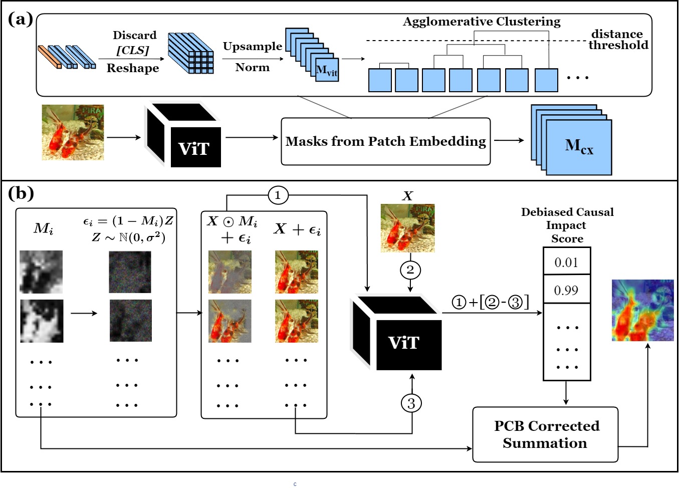
Figure 3: Overview of ViT-CX. (a) Mask Generation: A set of semantic masks is generated from the patch embeddings with agglomerative clustering. (b) Mask Aggregation: A saliency map is created by combining the masks using a debiased causal impact score based on the masked image with randomness to overcome artifacts. Pixel coverage frequencies are used in this step to correct pixel coverage bias.

2.2 Mask-based Explanation Methods

While there are only a few methods for explaining ViT models, a large number of methods have been proposed to explain CNN models. Mask-based explanation methods are one subclass. They generate an explanation based on a collection of masks $\mathbb{M}=\{M_{1},\cdots,M_{N}\}$, where each mask $M_{i}$ is of the same size as the input image $X$, and its pixel values are between 0 and 1. A saliency map, as an explanation, is created by aggregating the masks weighted by causal impacts of masks on the model output. Intuitively, we can think of a mask $M_{i}$ as a “pixel team”, and the saliency value of a pixel is an aggregation of the causal impact scores of “teams” it is on. Occlusion Zeiler and Fergus (2014), RISE Petsiuk et al. (2018) and Score-CAM Wang et al. (2020) are typical mask-based explanation methods.

In mask-based explanation methods, the causal impact of a mask is usually measured by the class score ($f(\cdot)$) of the masked image $X\odot M_{i}$ on the target class $y$. The saliency value of a pixel $x$ is determined by:

$$S(x)=\sum_{i=1}^{N}f(y|X\odot M_{i})M_{i}(x).$$ (1)

For visualization, the saliency values are normalized to interval $[0,1]$ by $(S(x)-\min_{x}S(x))/(\max_{x}S(x)-\min_{x}S(x)$.

Score-CAM is a mask-based explanation method proposed to CNNs. It uses CNN feature maps as masks. One can apply it to ViTs by replacing CNN feature maps with ViT feature maps. However, this simple adaptation does not lead to quality explanations. ViT-CX improves it significantly by taking into account characteristics of ViTs.

ViT Shapley Covert et al. (2022) is another mask-based explanation for ViTs proposed very recently. It trains a separate explainer (another ViT model) to estimate the Shapley Values. ViT Shapley has been evaluated only on small datasets (ImageNette and MURA) because the cost of training the explainer is high. Its performance on large datasets such as ImageNet is difficult to assess. In addition, the explainer is a black-box and it introduces new opacity which might need further explanation.

3 ViT-CX

An overview of ViT-CX is shown in Figure 3. ViT-CX follows the two-phase setting of mask-based explanation methods: mask generation followed by the mask aggregation. In the first phase, a small set of semantic masks is generated from the patch embeddings in the target ViT model with a clustering algorithm applied to reduce the number and redundancy of masks (Section 3.2). In the second phase, we propose a debiased causal impact score to overcome the artifact bias (Section 3.3.3), and the final saliency map is obtained by pixel coverage bias corrected summation (Section 3.4).

3.1 Preliminaries

In ViT models, an image $X\in\mathbb{R}^{H\times W\times C}$ is split into $N=HW/p^{2}$ patches, with the $j$-th patch represented by a 2D vector $X_{j}\in\mathbb{R}^{(p\times p)\times C}$, where $H,W,C$ are the height, width, and the number of channels of the image, and $(p,p)$ is the spatial resolution of each patch. The patches are mapped to embeddings with $D$ dimensions via linear projection. The embeddings are fed into $L$ transformer blocks. Each block includes two modules: A Multi-Head Self-Attention (MHSA) module and a Multi-Layer Perceptron (MLP) module. They yield new embeddings of the patches. We denote the patch embeddings at the output of transformer block $i$ as ${E}^{(i)}\in\mathbb{R}^{N_{i}\times D_{i}}$, where $N_{i}$ is the number of patch tokens and $D_{i}$ is the feature dimension at that block. The $N_{i}$ and $D_{i}$ remain constant in vanilla ViT Dosovitskiy et al. (2020) as the computation proceeds from one block to another, and are gradually changed in the more recent ViTs Wang et al. (2021); Chu et al. (2021); Liu et al. (2021) with hierarchical structures.

3.2 Mask Generation

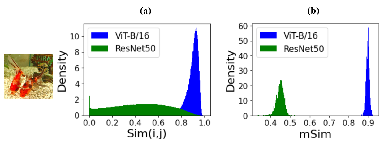
Figure 4: ViT masks has lower variance then CNN masks. (a) Distribution of pairwise similarities ($Sim(i,j)$) between masks for the goldfish image; (b) Distribution of mean pairwise mask similaritiy ($mSim$) for all images in the ImageNet validation set.

3.2.1 From ViT Feature Maps to ViT Masks

We create the masks from the embeddings ${E}^{(i)}$ at the output of the attention module of a chosen transformer block $i$ (usually the last transformer block for the vanilla ViT and possibly other block(s) for other ViT models). The embeddings are first reshaped into a 3D tensor of size $\sqrt{N_{i}}\times\sqrt{N_{i}}\times D_{i}$. Each fiber in the tensor corresponds to the embedding of a patch, and the $(x,y)$-coordinates correspond to the spatial location of the patch in the input image. The frontal slices of the tensor are upsampled to the size of the input image, resulting in the ViT feature maps. The feature maps are subsequently normalized to the interval $[0,1]$ to get ViT masks. A set of masks is built from those ViT masks, denoted as $\mathbb{M}_{vit}=\{M_{1},\cdots,M_{D_{i}}\}$ where $M_{j}\in R^{H\times W}$ ($j=1,\cdots,D_{i}$). The number of masks in $\mathbb{M}_{vit}$ is $D_{i}$ ($D_{i}=768$ in ViT-B/16).

3.2.2 High Degree of Redundancy in ViT Masks

We observe a high degree of redundancy among the ViT masks. This is clear from Figure 2 (c.1 - c.5). To quantify the level of redundancy among ViT masks, we compute the pairwise cosine similarity between the mask $M_{i}$ and $M_{j}$: $Sim(i,j)=\frac{M_{i}}{||M_{i}||}\boldsymbol{\cdot}\frac{M_{j}^{T}}{||M_{j}||}$.

The mean pairwise cosine similarity $mSim$ is defined as: $mSim={\sum_{i=1}^{D_{i}}\sum_{j=i+1}^{D_{i}}{Sim}(i,j)}/[{D_{i}(D_{i}-1)/2}]$. There is a high average $mSim$ for the mask set $\mathbb{M}_{vit}$ obtained from the last transformer block of ViT-B/16 - 0.92 , and the probability density distribution of the $mSim$ over images in ImageNet validation set is shown in Figure 4 (b). Figure 4 (a) shows the distribution of pairwise similarities $Sim(i,j)\ \ (j>i)$ for the goldfish image, indicating most ViT masks of this image are close to each other. This points to the possibility of clustering similar ViT masks together to improve the explanation efficiency.

In contrast, there is much more variance among CNN masks. This is clear from Figure 4 where we also show the probability density distribution of masks $\mathbb{M}_{resnet}$ from a popular CNN, ResNet50 He et al. (2016). Given that most masks are not similar to each other in $\mathbb{M}_{resnet}$, applying the clustering on it can force the dissimilar masks to be grouped and cause a significant information loss.

3.2.3 Clustering the ViT Masks

To reduce the redundancy in the mask set and improve the explanation efficiency, we merge the similar ViT masks. We use the agglomerative clustering algorithm Müllner (2013); Murtagh and Legendre (2014) which recursively merges data points with minimum pairwise distance. The pairwise distance of the mask $M_{i}$ and $M_{j}$ is measured by:

$$Distance(i,j)=1-\frac{M_{i}}{||M_{i}||}\boldsymbol{\cdot}\frac{M_{j}^{T}}{||M_{j}||}\ .$$

We stop the recursive merging based on a given distance threshold $\delta$ above which clusters will not be merged. Suppose the masks in $\mathbb{M}_{vit}$ is clustered into $K$ groups and each group is denoted as $\mathbb{M}_{vit}^{(k)}$ ($k=1,2,\cdots,K$). Here $K$ is different for different images depending on the distribution of their ViT feature maps. We take the mean of the masks in each group to build the mask set $\mathbb{M}_{cx}$ used in ViT-CX:

$$\mathbb{M}_{cx}=\{{M}_{1},{M}_{2},\cdots,{M}_{K}\},$$

$$\text{where }{M}_{k} =\frac{1}{|\mathbb{M}_{vit}^{(k)}|}\sum_{M\in\mathbb{M}_{vit}^{(k)}}M\ \text{, and }k=1,\cdots,K.$$

After the clustering, the number of masks decreases a lot ($K$ is 63 on average after clustering the previous $\mathbb{M}_{vit}$ with $\delta=0.1$). The reduction in the number of masks reduces the number of “pixel teams” that we need to investigate the causal impact for and thus can improve the online efficiency. At the same time, we show in Section 5 that reducing the amount of “pixel teams” in this way has only a slight impact on the explanation quality.

3.3 Artifacts and Debiased Causal Impact Score

Input:  P(g)=0.998

ViT Feature Map ViT Mask Masked Image Masked Image with Noise Image with Noise $M_{i}$ $X\odot M_{i}$ $X\odot M_{i}+\epsilon_{i}$ $X+\epsilon_{i}$ Case (a) P(g)=0.973 P(g)=0.005 P(g)=0.991 Original CI = $\mathit{0.973}$, Debiased CI = $\mathbf{0.012}$ Case (b) P(g)=0.994 P(g)=0.981 P(g)=0.986 Original CI = $\mathit{0.994}$, Debiased CI = $\mathbf{0.993}$

Figure 5: Comparison of the original causal impact score (CI) and the proposed debiased causal impact score on the goldfish (g) example. The original impact score is the prediction score of target class $y$ on the masked image - $f(y|X\odot M_{i})$. The proposed debiased impact score based on masked images with randomness aims to address the artifact case (case (a)) where the masked pixels lead to misleading $f(y|X\odot M_{i})$. Meanwhile the causal impact score in the normal case (case (b)) is not affected.

3.3.1 Artifactual Effects of Masked Pixels

Considering the mask $M_{i}$ as a “pixel team”, an implicit assumption in mask-based explanations is that only members of the “pixel team” contribute to the causal impact score, while non-member pixels do not.

In previous mask-based explanation methods, the causal impact score of a mask is usually measured by the prediction score of target class $y$ on the masked image - $f(y|X\odot M_{i})$, which can be problematic for ViTs. This problem arises from the violation of the implicit assumption. The masked pixels, as non-members of the “pixel team”, are at the same zero pixel value. They can co-create artifact that provides inferable information to the model and contributes strongly to the causal impact score, leading to the biased impact score.

Figure 5 case (a) shows an example of the artifact. The ViT feature map focuses on the background rather than the foreground, where the foreground pixels (goldfish’s pixels) share the least salient values. When the ViT mask is combined with the image, the foreground pixels are masked out. This erases the detailed features of the goldfish, such as texture and color. However, the masked pixels together create the shape of the goldfish in the masked image, resulting in an unreasonably high prediction score of goldfish - 0.973. This phenomenon might relate to the stronger shape recognition ability of ViTs when making the inference, as pointed out by Naseer et al. (2021); Tuli et al. (2021).

3.3.2 Noise Addition to Correct Artifact Bias

To correct the artifact bias, we need to corrupt the information from the masked pixels with the same zero pixel values. This corruption can be achieved by adding random noise to these pixels. Therefore we propose to add the random noise in a soft way to the masked image: $X\odot M_{i}+(1-M_{i})Z$ , where $Z\in\mathbb{R}^{H\times W\times C}$ follows a Gaussian distribution $\mathbb{N}(0,\sigma^{2})$ with a small standard deviation $\sigma$. Adding the noise based on the complement of mask values, i.e., $(1-M_{i})$, allows only the distribution of masked pixels (non-member pixels) to be mainly affected while the distribution of pixels with the highest mask values (pixels in the “team”) is minimally affected. In Figure 5 (a), after the noise is added, the prediction score of goldfish drops to 0.005. In case (b) where the goldfish body is preserved perfectly after masking, adding noises only makes the prediction score drop a tiny bit (0.994 $\rightarrow$ 0.981).

3.3.3 Debiased Causal Impact Score

Based on random noise addition, to reduce the effect of artifacts, we replace the term $f(y|X\odot M_{i})$ in Equation (1) with a debiased version of causal impact score:

$$s(X,y,M_{i})=$$

$$f(y|X\odot M_{i}+\epsilon_{i})+[f(y|X)-f(y|X+\epsilon_{i})],$$

(2)

$$\text{where }\epsilon_{i}=(1-M_{i})Z\in\mathbb{R}^{H\times W\times C},Z\sim\mathbb{N}(0,\sigma^{2}).$$

In Equation (2), the term $[f(y|X)-f(y|X+\epsilon_{i})]$ is the drop on the prediction score of target class $y$ when the random noise is added to the unmasked image. We add this term to cancel the effect of the random noise addition and ensure the resulting scores purely reflect the effect of the masks $M_{i}$ on the image. The use of Equation (2) as the causal impact score when explaining ViTs is a good solution to the case of artifacts caused by the masked pixels, as the examples shown in Figure 5. The ablation study in Section 5 shows the effectiveness of this debiased score in more general cases.

3.4 Pixel Coverage Bias and Its Correction

Given the set of masks $\mathbb{M}_{cx}=\{M_{1},M_{2},\cdots,M_{K}\}$, the coverage frequency of a pixel $x$ is defined as:

$$\rho(x)=\frac{1}{K}\sum_{i=1}^{K}M_{i}(x).$$

Pixel coverage bias (PCB) refers to the phenomenon that different pixels might have different coverage frequencies. According to Equation (1), the saliency value of a pixel, before being normalized to $[0,1]$, is the summation of the causal impact scores of the “pixel teams” (masks) of which it is a member. Consequently, the more “teams” a pixel on, the higher its saliency value. This is clearly not justified.

3.4.1 Adverse Effects of PCB

Although pixel coverage bias is a common issue in mask-based explanation methods, it does not necessarily cause severe degradation in explanation quality. However, it can severely degrade explanation quality in the cases of causal overdetermination. In those cases, the correct prediction can be made by various small patches of the input image White et al. (2021), resulting that the causal impact score $s(X,y,{M}_{i})$ of most masks is close to 1. To understand why PCB can cause undesirable explanation results in such cases, we let $\mu=\frac{1}{K}\sum_{i=1}^{K}s(X,y,{M}_{i})$ and $\beta_{i}=s(X,y,{M}_{i})-\mu$, and divide the saliency score $S(x)$ of a pixel into two parts:

$$S(x) = \sum_{i=1}^{K}\beta_{i}{M}_{i}(x)+\sum_{i=1}^{K}\mu{M}_{i}(x)$$ (3)

$$= \sum_{i=1}^{K}\beta_{i}{M}_{i}(x)+\mu K\rho(x).$$ (4)

In the overdetermined cases, the $\mu$ (mean of impact scores) is close to 1, but $\beta_{i}$ is small for most $i$’s. Thus the second term, which is essentially the pixel coverage frequency, is much larger than the first term. When normalized to the interval $[0,1]$, the first term basically vanishes. That leads to the saliency maps closely resemble the coverage frequency maps and fail to highlight areas important to the ViT prediction. One example of such case is given in Figure 6.

(a)	(a.1)	(a.2)	(a.3)

Figure 6: Impact of PCB: The nonsensical saliency map (a.2) closely resembles the coverage frequency map (a.1). After PCB correction, the map (a.3) becomes meaningful (target class - dogsled).

3.4.2 Causal Overdetermination in ViTs

Causal overdetermination is common with ViTs. We find 20.95% of the images in ImageNet validation set have a mean causal impact score $\mu$ greater than 0.9 when applying the mask $\mathbb{M}_{cx}$ to explain ViT/B-16. Among those images, the average variance of the score is 0.036, which is small. They fit the features of high $\mu$ and low $\beta_{i}$ mentioned above. This finding is also consistent with Naseer et al. (2021)’s observation that the class scores in ViTs are more robust to the removal of small patches in the input image than many popular CNNs.

		ViT-B			DeiT-B			Swin-B
	Del $\downarrow$	Ins $\uparrow$	PG Acc $\uparrow$	Del $\downarrow$	Ins $\uparrow$	PG Acc $\uparrow$	Del $\downarrow$	Ins $\uparrow$	PG Acc $\uparrow$
ViT-CX	0.161	0.620	86.42%	0.211	0.802	86.93%	0.271	0.761	92.31%
Number of Masks	Average: 63, Std: 11			Average: 70, Std:12			Average: 95, Std:12
Rollout	0.251	0.517	60.91%	0.406	0.642	35.70%	—	—	—
Partial LRP	0.239	0.499	66.52%	0.349	0.655	61.25%	—	—	—
CGW1	0.201	0.542	77.14%	0.286	0.717	70.54%	—	—	—
CGW2	0.209	0.549	70.94%	0.271	0.736	70.54%	—	—	—
TAM	0.180	0.556	77.87%	0.240	0.747	75.47%	—	—	—
Occlusion	0.291	0.571	64.75%	0.380	0.801	59.51%	0.448	0.752	69.65%
RISE	0.234	0.581	73.30%	0.366	0.759	71.84%	0.416	0.727	75.07%
Score-CAM	0.291	0.471	48.89%	0.439	0.576	50.12%	0.424	0.641	69.65%
Grad-CAM	0.212	0.456	50.45%	0.250	0.743	79.24 %	0.356	0.693	88.46%
Integrated-Grad	0.184	0.263	10.61%	0.259	0.362	10.74%	0.420	0.483	7.69%
Smooth-Grad	0.174	0.438	16.96%	0.231	0.528	31.05%	0.369	0.505	14.52%

Table 1: Main experiment results: Boldface and underline indicate best and second best performance, and ‘—’ means not applicable. ViT-CX significant outperforms all baselines in terms of the faithfulness metrics deletion (Del) and insertion AUC (Ins), and in terms of the interpretability metric Pointing Game Accuracy (PG Acc). The average number of masks ViT-CX used to explain an image is also provided.

3.4.3 Correction for PCB

A simple way to correct for PCB is to divide the saliency value $S(x)$ by the coverage frequency $\rho(x)$. This results in the corrected saliency value:

$$S^{c}(x)=\frac{S(x)}{\rho(x)}=\sum_{i=1}^{K}s(X,y,{M}_{i})\frac{{M}_{i}(x)}{\rho(x)}\ ,$$ (5)

where $S^{c}(x)=0$ by definition when $\rho(x)=0$. Intuitively, the corrected saliency value of a pixel is the sum of the causal impact scores of the “teams” of which it is a member, divided by the number of “teams” it participates in. Similar to Equation (4), we decompose $S^{c}(x)$ into two parts:

$$S^{c}(x)=\sum_{i=1}^{K}\beta_{i}\frac{{M}_{i}(x)}{\rho(x)}+\mu K.$$ (6)

The second term is still much larger than the first term. However, it is a constant and does not depend on the pixel. When the saliency values $S^{c}(x)$ are normalized to the interval $[0,1]$ for visualization, the influence of the second term is wholly eliminated. This is why meaningful saliency maps emerge in Figure 6 after correcting for PCB. In Section 5.4, we show the correction improves the overall explanation quality greatly.

This correction is also included in Petsiuk et al. (2018) and Sattarzadeh et al. (2021). Their motivation is to correct the bias caused by the finiteness of random sampling. We here provide another viewpoint on it and show its importance in causal overdetermination cases.

4 Experiments

4.1 Evaluation Metrics

We evaluate ViT-CX following a protocol similar to how previous ViT explanation methods are evaluated, using the Deletion and Insertion AUC Petsiuk et al. (2018), Pointing Game Zhang et al. (2018) and visual examples. This scheme is commonly used to evaluate explanation methods for CNNs.

Deletion and Insertion AUC:

The two metrics are about the faithfulness of an explanation (saliency map) to the target model, i.e., whether pixels with high saliency values are really important to the prediction Petsiuk et al. (2018). Deletion AUC measures how fast the score of the target class drops as pixels are deleted from the image in descending order of the saliency values. Insertion AUC measures how fast the score increases when pixels are inserted into an empty canvas in that order. Smaller deletion AUC and larger insertion AUC indicate better faithfulness.

Pointing Game:

This metric is about the interpretability of an explanation, i.e., whether it provides qualitative understanding between input and output Ribeiro et al. (2016); Doshi-Velez and Kim (2017). In Pointing Game, the saliency maps are compared with human-annotated bounding boxes. For each pair of saliency map and bounding box, if the pixel with the highest saliency value falls inside the box, it is considered a hit. Otherwise it is considered a miss. The Pointing Game Accuracy is defined as: $Acc={\#Hits}/({\#Hits+\#Misses})$.

		Masks	Causal Impact	PCB	Number of Masks	Del $\downarrow$	Ins $\uparrow$	PG Acc $\uparrow$	Average Time (s)
ViT-CX	$\mathbb{M}_{cx}$	$s(X,y,M_{i})$	$\surd$	70 $\pm$ 12	0.211	0.802	86.93%	1.15 $\pm$ 0.15
Variant 1		$\mathbb{M}_{vit}$	$s(X,y,M_{i})$	$\surd$	768 $\pm$ 0	0.232	0.810	85.52%	8.23 $\pm$ 0.03
Variant 2	$\mathbb{M}_{random}$	$s(X,y,M_{i})$	$\surd$	5000 $\pm$ 0	0.323	0.734	75.12%	77.78 $\pm$ 3.46
Variant 3		$\mathbb{M}_{cx}$	$f(y|X\odot M_{i})$	$\surd$	70 $\pm$ 12	0.281	0.742	77.78%	0.98 $\pm$ 0.12
Variant 4	$\mathbb{M}_{cx}$	$s(X,y,M_{i})$	$\times$	70 $\pm$ 12	0.303	0.727	74.37%	1.12 $\pm$ 0.14
Variant 5	$\mathbb{M}_{cx}$	$f(y|X\odot M_{i})$	$\times$	70 $\pm$ 12	0.339	0.686	67.56%	0.95 $\pm$ 0.08

Table 2: Ablation study on ViT-CX (based on DeiT-B, GPU batch size=100). The analyzed components include: 1. Masks - the mask set used in the explanation. $\mathbb{M}_{cx}$ is generated from ViT feature maps with reduced number by clustering and $\mathbb{M}_{vit}$ is the one without clustering. $\mathbb{M}_{random}$ is randomly generated; 2. Causal Impact - the measure of casual impact of the mask. $s(X,y,M_{i})$ is our proposed debiased causal impact score and $f(y|X\odot M_{i})$ is the prediction score of masked image; 3. PCB - whether to apply the PCB correction.

4.2 Experiment Settings

Models and Dataset: Three ViT variants are used in our experiments: (1) ViT-B/16 Dosovitskiy et al. (2020), the vanilla ViT; (2) DeiT-B/16-Distill Touvron et al. (2021), a improved version of the vanilla ViT with a distillation token; (3) Swin-B Liu et al. (2021), a hierarchical ViT. We use 5,000 images randomly selected from the ILSVRC2012 validation set Deng et al. (2009). All experiments are run on an Intel Xeon E5-2620 CPU and an NVIDIA 2080 Ti GPU.

Hyper-parameters Setting:

To generate the masks $\mathbb{M}_{vit}$, we use feature maps from the last transformer block for ViT-B and DeiT-B, and choose those from the last block of the second to last stage for Swin-B; When clustering on $\mathbb{M}_{vit}$ to generate the mask set $\mathbb{M}_{cx}$, the distance threshold $\delta$ is set to 0.1 for ViT-B and DeiT-B, and set to 0.05 for Swin-B; The standard deviation $\sigma$ of the Gaussian noise $\epsilon_{i}$ is set to 0.1.

Baselines:

In this section, we compare ViT-CX with three groups of baselines: (a) Five attention weights-based methods, namely Rollout Abnar and Zuidema (2020), Partial LRP Voita et al. (2019), CGW1 Chefer et al. (2021b), CGW2 Chefer et al. (2021a), and TAM Yuan et al. (2021); (b) Three mask-based methods, namely Occlusion Zeiler and Fergus (2014), RISE Petsiuk et al. (2018) and Score-CAM Wang et al. (2020); (c) Three gradient-based methods, namely Grad-CAM Selvaraju et al. (2017), Integrated-Grad Sundararajan et al. (2017) and Smooth-Grad Smilkov et al. (2017). In addition, Appendix D provides a comparison between ViT-CX and ViT Shapley, a mask-based explanation method for ViTs introduced in a recent study by Covert et al. (2022).

4.3 Results

The main results are in Table 1.

Faithfulness:

ViT-CX has the lowest deletion AUC values across the board, being 10% lower than the next best. ViT-CX also enjoys the highest insertion AUC values in all cases. Those indicate that ViT-CX is more faithful to the target models than all baselines.

Interpretability:

ViT-CX enjoys significantly higher Pointing Game accuracy than the baselines in all cases. This implies that the explanations of ViT-CX are more consistent with human-annotated bounding boxes. As a supplement to quantitative metrics, four visual examples have been shown in Figure 1 and more examples are given in Appendix A.

Computation Cost:

ViT-CX uses less than 100 masks on average to explain an image. The computation cost is greatly reduced compared to previous mask-based methods.

Sanity Check:

As a causal method, ViT-CX is sensitive to the changes in model parameters and passes the sanity check Adebayo et al. (2018). See Appendix B for details.

Localization:

As a training-free method, ViT-CX shows comparable localization performance to recently proposed ViT-based weakly supervised object localizers that require extra modules and training. The details are in Appendix C.

4.4 Ablation Study

The collection of masks used in the explanation, the causal impact score, and whether the PCB correction is applied are varied to study the effect of different components in ViT-CX. The results are in Table 2.

Comparison of ViT-CX with Variant 1 shows that clustering on the mask set $\mathbb{M}_{vit}$ reduces the number of masks from 768 to 70 on average, and the mean time to explain an image is reduced to $\sim$1 second. Meanwhile the explanation quality is mainly remained unaffected. Additionally, ViT-CX outperforms explanations generated with random masks (Variant 2) in terms of explanation quality and efficiency.

Comparisons with Variants 3-5 emphasize the significance of addressing pixel coverage bias and using a debiased causal impact score in ViT-CX to avoid artifact effects. Without these steps, the explanation quality is largely affected. These results suggest that the clustering of masks, the correction for PCB and the debiasing of causal impact scores are crucial components of ViT-CX. A more detailed sensitivity analysis of hyperparameters in ViT-CX can be found in Appendix F.

5 Conclusion

Previous attention weights-based and mask-based explainers have not been able to consistently provide satisfactory explanations for ViTs. ViT-CX, a specially designed mask-based explainer for ViTs, addresses the issues of low explanation efficiency, misleading causal impact scores caused by artifacts, and pixel coverage bias of masks. Our solutions to these issues are demonstrated to lead to high-quality explanations for various ViT image classifiers. Future work could involve extending ViT-CX concepts to explain ViT models for other tasks like object detection and segmentation.

Contribution Statement

Weiyan Xie and Xiao-Hui Li contributed equally to this work. This work is done when Caleb Chen Cao was in Huawei Research Hong Kong.

References

- Abnar and Zuidema [2020] Samira Abnar and Willem Zuidema. Quantifying attention flow in transformers. In Annual Meeting of the Association for Computational Linguistics, pages 4190–4197, 2020.
- Adebayo et al. [2018] Julius Adebayo, Justin Gilmer, Michael Muelly, Ian Goodfellow, Moritz Hardt, and Been Kim. Sanity checks for saliency maps. In Advances in Neural Information Processing Systems, pages 9525–9536, 2018.
- Bach et al. [2015] Sebastian Bach, Alexander Binder, Grégoire Montavon, Frederick Klauschen, Klaus-Robert Müller, and Wojciech Samek. On pixel-wise explanations for non-linear classifier decisions by layer-wise relevance propagation. PloS one, 10(7):e0130140, 2015.
- Bastings and Filippova [2020] Jasmijn Bastings and Katja Filippova. The elephant in the interpretability room: Why use attention as explanation when we have saliency methods? In Proceedings of the Third BlackboxNLP Workshop on Analyzing and Interpreting Neural Networks for NLP, pages 149–155, 2020.
- Carion et al. [2020] Nicolas Carion, Francisco Massa, Gabriel Synnaeve, Nicolas Usunier, Alexander Kirillov, and Sergey Zagoruyko. End-to-end object detection with transformers. In European conference on computer vision, pages 213–229. Springer, 2020.
- Chefer et al. [2021a] Hila Chefer, Shir Gur, and Lior Wolf. Generic attention-model explainability for interpreting bi-modal and encoder-decoder transformers. In Proceedings of the IEEE/CVF International Conference on Computer Vision, pages 397–406, 2021.
- Chefer et al. [2021b] Hila Chefer, Shir Gur, and Lior Wolf. Transformer interpretability beyond attention visualization. In Proceedings of the IEEE/CVF conference on computer vision and pattern recognition, pages 782–791, 2021.
- Chu et al. [2021] Xiangxiang Chu, Zhi Tian, Yuqing Wang, Bo Zhang, Haibing Ren, Xiaolin Wei, Huaxia Xia, and Chunhua Shen. Twins: Revisiting the design of spatial attention in vision transformers. Advances in Neural Information Processing Systems, 34:9355–9366, 2021.
- Covert et al. [2022] Ian Covert, Chanwoo Kim, and Su-In Lee. Learning to estimate shapley values with vision transformers. arXiv preprint arXiv:2206.05282, 2022.
- Deng et al. [2009] Jia Deng, Wei Dong, Richard Socher, Li-Jia Li, Kai Li, and Li Fei-Fei. Imagenet: A large-scale hierarchical image database. In Proceedings of the IEEE/CVF conference on computer vision and pattern recognition, pages 248–255. Ieee, 2009.
- Doshi-Velez and Kim [2017] Finale Doshi-Velez and Been Kim. Towards a rigorous science of interpretable machine learning. arXiv preprint arXiv:1702.08608, 2017.
- Dosovitskiy et al. [2020] Alexey Dosovitskiy, Lucas Beyer, Alexander Kolesnikov, Dirk Weissenborn, Xiaohua Zhai, Thomas Unterthiner, Mostafa Dehghani, Matthias Minderer, Georg Heigold, Sylvain Gelly, et al. An image is worth 16x16 words: Transformers for image recognition at scale. In International conference on learning representations, 2020.
- He et al. [2016] Kaiming He, Xiangyu Zhang, Shaoqing Ren, and Jian Sun. Deep residual learning for image recognition. In Proceedings of the IEEE/CVF conference on computer vision and pattern recognition, pages 770–778, 2016.
- Jain and Wallace [2019] Sarthak Jain and Byron C Wallace. Attention is not explanation. In Proceedings of NA Annual Meeting of the Association for Computational Linguistics-HLT, pages 3543–3556, 2019.
- Liu et al. [2021] Ze Liu, Yutong Lin, Yue Cao, Han Hu, Yixuan Wei, Zheng Zhang, Stephen Lin, and Baining Guo. Swin transformer: Hierarchical vision transformer using shifted windows. In Proceedings of the IEEE/CVF International Conference on Computer Vision, pages 10012–10022, 2021.
- Müllner [2013] Daniel Müllner. fastcluster: Fast hierarchical, agglomerative clustering routines for r and python. Journal of Statistical Software, 53:1–18, 2013.
- Murtagh and Legendre [2014] Fionn Murtagh and Pierre Legendre. Ward’s hierarchical agglomerative clustering method: which algorithms implement ward’s criterion? Journal of classification, 31(3):274–295, 2014.
- Naseer et al. [2021] Muzammal Naseer, Kanchana Ranasinghe, Salman Khan, Munawar Hayat, Fahad Khan, and Ming-Hsuan Yang. Intriguing properties of vision transformers. In Advances in Neural Information Processing Systems, 2021.
- Petsiuk et al. [2018] Vitali Petsiuk, Abir Das, and Kate Saenko. Rise: Randomized input sampling for explanation of black-box models. In Proceedings of the British Machine Vision Conference, 2018.
- Pruthi et al. [2020] Danish Pruthi, Mansi Gupta, Bhuwan Dhingra, Graham Neubig, and Zachary C Lipton. Learning to deceive with attention-based explanations. In Annual Meeting of the Association for Computational Linguistics, pages 4782–4793, 2020.
- Ribeiro et al. [2016] Marco Tulio Ribeiro, Sameer Singh, and Carlos Guestrin. ” why should i trust you?” explaining the predictions of any classifier. In Proceedings of the ACM SIGKDD international conference on knowledge discovery and data mining, pages 1135–1144, 2016.
- Sattarzadeh et al. [2021] Sam Sattarzadeh, Mahesh Sudhakar, Anthony Lem, Shervin Mehryar, Konstantinos N Plataniotis, Jongseong Jang, Hyunwoo Kim, Yeonjeong Jeong, Sangmin Lee, and Kyunghoon Bae. Explaining convolutional neural networks through attribution-based input sampling and block-wise feature aggregation. In Proceedings of the AAAI Conference on Artificial Intelligence, volume 35, pages 11639–11647, 2021.
- Selvaraju et al. [2017] Ramprasaath R Selvaraju, Michael Cogswell, Abhishek Das, Ramakrishna Vedantam, Devi Parikh, and Dhruv Batra. Grad-cam: Visual explanations from deep networks via gradient-based localization. In Proceedings of the IEEE/CVF International Conference on Computer Vision, pages 618–626, 2017.
- Serrano and Smith [2019] Sofia Serrano and Noah A Smith. Is attention interpretable? In Annual Meeting of the Association for Computational Linguistics, pages 2931–2951, 2019.
- Smilkov et al. [2017] Daniel Smilkov, Nikhil Thorat, Been Kim, Fernanda Viégas, and Martin Wattenberg. Smoothgrad: removing noise by adding noise. arXiv preprint arXiv:1706.03825, 2017.
- Sundararajan et al. [2017] Mukund Sundararajan, Ankur Taly, and Qiqi Yan. Axiomatic attribution for deep networks. In International Conference on Machine Learning, pages 3319–3328. PMLR, 2017.
- Touvron et al. [2021] Hugo Touvron, Matthieu Cord, Matthijs Douze, Francisco Massa, Alexandre Sablayrolles, and Hervé Jégou. Training data-efficient image transformers & distillation through attention. In International Conference on Machine Learning, pages 10347–10357. PMLR, 2021.
- Tuli et al. [2021] Shikhar Tuli, Ishita Dasgupta, Erin Grant, and Tom Griffiths. Are convolutional neural networks or transformers more like human vision? In Proceedings of the Annual Meeting of the Cognitive Science Society, volume 43, 2021.
- Voita et al. [2019] Elena Voita, David Talbot, Fedor Moiseev, Rico Sennrich, and Ivan Titov. Analyzing multi-head self-attention: Specialized heads do the heavy lifting, the rest can be pruned. In Annual Meeting of the Association for Computational Linguistics, pages 5797–5808. Annual Meeting of the Association for Computational Linguistics Anthology, 2019.
- Wang et al. [2020] Haofan Wang, Zifan Wang, Mengnan Du, Fan Yang, Zijian Zhang, Sirui Ding, Piotr Mardziel, and Xia Hu. Score-cam: Score-weighted visual explanations for convolutional neural networks. In Proceedings of the IEEE/CVF conference on computer vision and pattern recognition workshop, pages 24–25, 2020.
- Wang et al. [2021] Wenhai Wang, Enze Xie, Xiang Li, Deng-Ping Fan, Kaitao Song, Ding Liang, Tong Lu, Ping Luo, and Ling Shao. Pyramid vision transformer: A versatile backbone for dense prediction without convolutions. In Proceedings of the IEEE/CVF International Conference on Computer Vision, pages 568–578, 2021.
- White et al. [2021] Adam White, Kwun Ho Ngan, James Phelan, Saman Sadeghi Afgeh, Kevin Ryan, Constantino Carlos Reyes-Aldasoro, and Artur d’Avila Garcez. Contrastive counterfactual visual explanations with overdetermination. arXiv preprint arXiv:2106.14556, 2021.
- Yuan et al. [2021] Tingyi Yuan, Xuhong Li, Haoyi Xiong, Hui Cao, and Dejing Dou. Explaining information flow inside vision transformers using markov chain. In eXplainable AI approaches for debugging and diagnosis., 2021.
- Zeiler and Fergus [2014] Matthew D Zeiler and Rob Fergus. Visualizing and understanding convolutional networks. In European conference on computer vision, pages 818–833. Springer, 2014.
- Zhang et al. [2018] Jianming Zhang, Sarah Adel Bargal, Zhe Lin, Jonathan Brandt, Xiaohui Shen, and Stan Sclaroff. Top-down neural attention by excitation backprop. Proceedings of the IEEE/CVF International Conference on Computer Vision, 126(10):1084–1102, 2018.
- Zhang et al. [2022] Zizhao Zhang, Han Zhang, Long Zhao, Ting Chen, Sercan Ö Arik, and Tomas Pfister. Nested hierarchical transformer: Towards accurate, data-efficient and interpretable visual understanding. In Proceedings of the AAAI Conference on Artificial Intelligence, volume 36, pages 3417–3425, 2022.