The Importance of Suppressing Complete Reconstruction in Autoencoders for Unsupervised Outlier Detection

Abstract

Autoencoders are widely used in outlier detection due to their superiority in handling high-dimensional and nonlinear datasets. The reconstruction of any dataset by the autoencoder can be considered as a complex regression process. In regression analysis, outliers can usually be divided into high leverage points and influential points. Although the autoencoder has shown good results for the identification of influential points, there are still some problems when detect high leverage points. Through theoretical derivation, we found that most outliers are detected in the direction corresponding to the worst-recovered principal component, but in the direction of the well-recovered principal components, the anomalies are often ignored. We propose a new loss function which solve the above deficiencies in outlier detection. The core idea of our scheme is that in order to better detect high leverage points, we should suppress the complete reconstruction of the dataset to convert high leverage points into influential points, and it is also necessary to ensure that the differences between the eigenvalues of the covariance matrix of the original dataset and their corresponding reconstructed results in the direction of each principal component are equal. Besides, we explain the rationality of our scheme through rigorous theoretical derivation. Finally, our experiments on multiple datasets confirm that our scheme significantly improves the accuracy of outlier detection.

1 Introduction

Outlier detection refers to the process of identifying data points that deviate significantly from normal data point clusters. Up to now, outlier detection has been wildly applied in diverse fields of science and technology, such as credit card transactions (Sivakumar & Balasubramanian, 2016; Nami & Shajari, 2018), intrusion detection (Aoudi et al., 2018), industrial control system inspection (Lin et al., 2018; Das et al., 2020), text detection (Mahapatra et al., 2012; Gorokhov et al., 2017) and outlier detection in biological data (Shetta & Niranjan, 2020; Tibshirani & Hastie, 2007; MacDonald & Ghosh, 2006). For multidimensional data points, there are various outliers. In the process of regression analysis, all outliers can be divided into two categories. One type of outliers is called influential points (IP), they have a huge influence on the fitting result of the model. Besides, the other type of outliers is called high leverage points (HLP), they deviate from the center of the dataset but do not necessarily have an effect on the model fit (Imon & Hadi, 2013).

According to whether the label information of the training dataset is required, outlier detection schemes can be divided into two types: supervised and unsupervised (Lu & Traore, 2005). For supervised outlier detection, the intrinsic information of the dataset is learned by training on the labeled dataset. However, in the unsupervised mode, there is no need to label the dataset in advance, and it is only necessary to assume that there are far more normal data points in the dataset than anomalies (Chandola et al., 2009). Since it’s difficult to obtain well-labeled datasets in practical applications or it will have huge consumption, nowadays, more and more studies have the preference to use unsupervised method. Up to now, there have been many unsupervised outlier detection schemes. PCA has been successfully used to detect outliers whose correlations between dimensions differ from normal points (Shyu et al., 2003). But it works worse when the correlations between different dimensions are nonlinear. KNN is another unsupervised outlier detection method, which is based on the distance of each data point to its nearest neighbor (Ramaswamy et al., 2000). LOF is proposed to find outliers based on density (Breunig et al., 2000). However, these two methods are less effective when the dimensionality of the dataset is high. Currently, in order to address the constraints of dimensionality and linearity, unsupervised outlier detection based on neural networks has attracted a great deal of attention.

Autoencoders are a type of neural network that has been successfully used for outlier detection in most researches (Lyudchik, 2016). The autoencoder first encodes the training dataset which are considered to be all normal into a low-dimensional space and then decodes them into the original space (Kim et al., 2020). The difference between a reconstructed value and its corresponding input value is the reconstruction error, and a low-dimensional representation of the training dataset can be learned by minimizing the reconstruction error. Finally, the trained autoencoder can be used to reconstruct the test dataset and measure the outlier degree of each data point according to its reconstruction error.

In the training process, to minimize the reconstruction error of the training dataset, most studies choose Mean Square Error (MSE) as the training loss function and force the autoencoder to completely reconstruct the training dataset (Antwarg et al., 2021). If a sample point cannot be reconstructed well, it will generate a large reconstruction error and finally be identified as an outlier. Besides, in the process of statistical regression analysis, IP are regarded as outliers because they have a great impact on the model fit. Since the reconstruction of any dataset by the autoencoder can be regarded as a process of regression, IP can be easily detected when using autoencoders for outlier detection. However, there are many uncertainties about the detection effect of HLP. To solve this problem, in our paper, we propose a new training loss function which properly suppress complete reconstruction of the autoencoder to convert HLP into IP to improve the detection effect of HLP.

In Section 2, we introduce the existing related research results of outlier detection with autoencoders and show the contributions in our paper. In Section 3, we highlight the importance of suppressing complete reconstruction of the autoencoder for outlier detection and conduct a theoretical analysis. Section 4 verifies the effectiveness of our scheme through presenting experimental results on both synthetic and real datasets. Section 5 summarizes the work of the paper and gives directions worthy of further study.

2 Related works and contribution

The main idea of outlier detection schemes based on reconstruction error is that normal data points can be well reconstructed, while outliers will generate large reconstruction errors (Bergman & Hoshen, 2020). In practical application, distance-based outlier detection methods (Ramaswamy et al., 2000; Kamoi & Kobayashi, 2020) and density-based approaches (Breunig et al., 2000; Liu et al., 2008) have problems of poor detection effect and large time cost when the dimension of the dataset is too high. Nowadays, many outlier detection schemes based on reconstruction error rely on neural network for reconstruction due to its high feature learning ability and the commonly used scheme is based on autoencoders (Lyudchik, 2016). Recently, there are also some studies use another neural network model GAN to detect outliers (Schlegl et al., 2017; Zenati et al., 2018).

Due to the strong representation learning and feature extraction capabilities, autoencoders are often used for outlier detection and have achieved fruitful research results. However, some studies have shown that the traditional autoencoder based outlier detection scheme still has defects, and there are some improvement can be made to significantly improve the outlier detection effect (Zhou & Paffenroth, 2017; Ning et al., 2022). Existing improvement schemes mainly focus on the structure and loss function of the autoencoder. In Lai et al. (2020), a robust subspace recovery layer is added to the autoencoder in order to make the results of outlier detection more robust to anomalies. Zhou & Paffenroth (2017) combines autoencoders with RPCA and adds an outlier regularizing penalty based on $l_{1}$ or $l_{2,1}$ norms to avoid the influence of noise on outlier detection results. Unfortunately, most existing work pursues complete reconstruction of the training dataset to improve anomaly detection effect. However, we reveal that complete reconstruction is not beneficial to identify HLP in this paper.

In our work, we improve outlier detection ability by properly suppressing complete reconstruction of the autoencoder to convert HLP into IP by improving the training loss function. Bao et al. (2020) and Oftadeh et al. (2020) reveal that autoencoders will eventually focus on recovering the principal components of a dataset, which indicates that the occurrence of complete reconstruction can be suppressed by suppressing the recovery of the principal components.

The main contributions of our work are as follows:

• Since the autoencoder can identify IP well but ignore the detection of HLP, we propose a new training loss function which properly suppress complete reconstruction of the training dataset and improve the detection effect of HLP while maintain the detection effect of IP. Therefore, the outliers detected by our scheme cover both HLP and IP. Besides, we also analyze how to determine the degree of reconstruction of the training dataset.

• Through rigorous theoretical analysis, we explain the detrimental effect of complete reconstruction on HLP detection, and show that properly suppressing complte reconstruction is beneficial for HLP detection.

• We test our outlier detection scheme on both synthetic and real datasets and confirm that our scheme improves the overall detection effect of outliers.

3 Method

In this section, we will start describing our new method for detecting outliers based on the autoencoder and its theoretical support. Our innovative idea is to properly suppress complete reconstruction of the autoencoder to convert HLP into IP to improve the detection effect of HLP. Firstly, we will introduce the restrictions of HLP detection with MSE-trained autoencoders. Then, we theoretically demonstrate the importance of suppressing complete reconstruction of the autoencoder. Finally, we propose a new training loss function and analyze how to properly suppress reconstruction.

3.1 Deficiencies of outlier detection with MSE-trained autoencoders

As is known, an autoencoder is a neural network formed of an encoder $f$ and a decoder $g$. If we denote the input data point and the output data point as variable $X$ and $\hat{X}$ respectively, where $X=\big{(}X_{1},X_{2},\ldots,X_{m}\big{)}^{\top}$ and $\hat{X}=\big{(}\hat{X}_{1},\hat{X}_{2},\ldots,\hat{X}_{m}\big{)}^{\top}$, and the number of sample points is $n$, then we have $\hat{X}=g\circ f(X)$. Besides, $\mathcal{X}$ represents the whole input dataset and $X\in\mathcal{X}$. $x_{i}$ represents the $i^{th}$ sample point of the input dataset and its corresponding reconstruction result is $\hat{x}_{i}$. Ideally, we would like to train the autoencoder with the training dataset to minimize the training loss function, the generally used training loss function is MSE which can be represented as

$$L_{MSE}(\omega,b)=\frac{1}{n}\sum_{i=1}^{n}(x_{i}-\hat{x}_{i})^{\top}(x_{i}-\hat{x}_{i}),$$

where $\omega$ represents the weight between the input layer and the output layer and $b$ is the bias value.

The purpose of training process is to guarantee that the intrinsic information of the training dataset can be learned and most of the sample data points can be well reconstructed. It should be pointed out that, although reconstructing training dataset well is beneficial for IP detection, it brings some problems to the detection of HLP:

• For each input data point, if in one dimension, its value is not in the expected range, it can be identified as an outlier. However, HLP whose values in each dimension are within the normal range can hardly be detected.

• If some principal components are recovered better than others, then more HLP will be detected along the direction of the poorly recovered principal components, while no HLP is even detected in the direction of the better recovered principal components.

Here, we will show the shortcomings of MSE-trained autoencoders for HLP detection with some examples. If the proportion of outliers is $5$ percent, we can see that the two deficiencies in HLP detection proposed above are prevalent in different datasets. As shown in Figure 1, we add non-Gaussian noise to the dataset to make the difference in detection efficiency of HLP in different principal component directions more obvious, and the orange line and grey line represent two principal directions. We can observe the distribution of HLP from Figure 1, most of the detected HLP lie in the direction of the principal components indicated by the grey line but few lie in the other principal direction. Besides, in Figure 1, we find almost all of the HLP are identified due to the value anomalous in one dimension. In Figure 1, 1 and 1, the training datasets are two dimensions and their intrinsic dimension are also two. Besides, the sample points follow two-dimensional Gaussian distribution. In Figure 1, the dimension of the dataset is three and the intrinsic dimension is two, the values of each dimension obey a Gaussian distribution. The structure of the autoencoder and the setting of hyperparameters are described in Section 4. Below we will explain that the effect of the saturation of the nonlinear activation functions on reconstruction lead to detection problems for HLP.

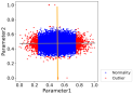
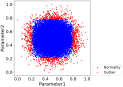
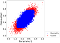
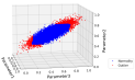
Figure 1: Examples of outlier detection with autoencoder when the loss function is MSE and the outlier ratio is $0.05$. In (a)-(c), the sample points follow two-dimensional Gaussian distribution. (a) Covariance matrix diagonal and non-Gaussian distributed noise exists, the orange line and grey line represent two principal directions. (b) Covariance matrix diagonal. (c) Covariance matrix off-diagonal. (d) The intrinsic dimension of the dataset is less than the actual dimension, and the values in each dimension follow a Gaussian distribution.

Usually, The dataset is normalized before being fed into the autoencoder, so the values of each dimension of the dataset are distributed in $(0,1)$. If we denote $F=g\circ f$, $F=(F_{1},F_{2},\ldots,F_{m})^{\top}$, since the output variable $\hat{X}$ and the input variable $X$ satisfy that $\hat{X}=F(X)$, for each dimension of the input variable, its corresponding reconstructuion result can be fomulated as $\hat{X}_{k}=F_{k}(X_{1},X_{2},\cdots,X_{m})$, $k=1,2,\ldots,m$. Furthermore, the total reconstruction error of each dimension is $\int_{0}^{1}\big{(}X_{k}-F_{k}(X_{1},X_{2},\cdots,X_{m})\big{)}^{2}dX_{k}$, ideally, $F_{k}(X_{1},X_{2},\cdots,X_{m})=X_{k}$ holds for almost all data points after reconstruction. Thus, we can conclude that $(i)$ For each dimension of the input dataset, $\hat{X}_{k}$ increases monotonically with $X_{k}$ and $\hat{X}_{k}\approx X_{k}$ holds for most data points after reconstruction. Figure 6(a) in Appendix B.1 can typically reflect the detection defect of the MSE-trained autoencoders for HLP. $(ii)$ Due to the saturation of the nonlinear activation functions of the output layer, in each dimension, values close to $0$ or close to $1$ are more difficult to reconstruct, and $\hat{X}_{k}$ cannot be approximated to $X_{k}$ in this case. In Figure 1, data points with large or small values in the direction of Parameter1 are identified as HLP. However, since values of Parameter2 of most data points significantly larger than $0$ or significantly smaller than $1$ and most of them are between $0.15$ and $0.85$, they can be reconstructed well. This makes it difficult to detect HLP in the direction of Parameter2. We choose the dataset in Figure 1 for further validation, see Appendix B.1.

3.2 The importance of suppressing complete reconstruction

In this part, we will present rigorous theoretical analysis to explain why MSE-trained autoencoders are insufficient in outlier detection, and further analyze how to solve these problems. The analysis process will be based on the following assumption.

Assumption 1.

Since most datasets follow a multidimensional Gaussian distribution, we assume that the input variable $X$ follows m-dimensional Gaussian distribution.

As we know, autoencoders will focus on recovering the principal components of a dataset eventually (Bao et al., 2020; Oftadeh et al., 2020), it is necessary to use the unit orthogonal eigenvectors as the basis vectors to further study the influence of the loss function on the outlier detection results of the autoencoder. Under Assumption 1, if the eigenvalues of the covariance matrix $\Sigma_{x}$ are $\lambda_{1}$, $\lambda_{2}$, $\ldots$, $\lambda_{m}$, the corresponding unit orthogonal eigenvectors (i.e., principal directions) are $\eta_{1}$, $\eta_{2}$, $\ldots$, $\eta_{m}$, and the new coordinate of the variable $X$ is $Y=\big{(}Y_{1},Y_{2},\ldots,Y_{m}\big{)}^{\top}$ when the unit orthogonal eigenvectors are the basis vectors, then we can denote an orthogonal matrix $P$, where the $i^{th}$ column of $P$ is unit eigenvector $\eta_{i}$. It’s obvious that $Y=P^{-1}X=P^{\top}X$ and $Y_{k}=\eta_{k}^{\top}X$, $k=1,2,\ldots,m$. Thus, in the new coordinate system, the variable of input data $X$ is converted to variable $Y$. Then we can get the formulation for the covariance matrix of variable $Y$ which will be proved in detail in Appendix A.1.

Result 1.

The covariance matrix of variable $Y$ can be derived as

$$\Sigma_{Y}={\rm diag}(\lambda_{1},\lambda_{2},\ldots,\lambda_{m}).$$

If we denote $\nu=(\nu_{1},\nu_{2},\ldots,\nu_{m})^{\top}$ as the mean vector of variable $Y$, since $X$ follows m-dimensional Gaussian distribution, we can conclude that $Y$ also follows m-dimensional Gaussian distribution, i.e., $Y$ $\sim$ $\mathcal{N}(\nu,\Sigma_{Y})$. What’s more, it’s easy to get that $Y_{k}$ $\sim$ $\mathcal{N}(\nu_{k},\lambda_{k})$, $k=1,2,\ldots,m$. Then, we denote $\hat{Y}$ as the output variable of $Y$ and its mean vector and eigenvalues of the covariance matrix are $\hat{\nu}=\big{(}\hat{\nu}_{1},\hat{\nu}_{2},\ldots,\hat{\nu}_{m}\big{)}^{\top}$ and $\hat{\lambda}_{k}$, $k=1,2,\ldots,m$, respectively. As is mentioned above, autoencoders will mainly recover the principal components of any datasets, it’s reasonable for us to make the following assumption.

Assumption 2.

For each element $\hat{Y}_{k}$ of the output variable $\hat{Y}$, its data distribution is the same as the corresponding input element $Y_{k}$. Since $Y_{k}$ $\sim$ $\mathcal{N}(\nu_{k},\lambda_{k})$, then $\hat{Y}_{k}$ $\sim$ $\mathcal{N}(\hat{\nu}_{k},\hat{\lambda}_{k})$, $k=1,2,\ldots,m$. Besides, whether each eigenvalue after reconstruction is close to 0 is the same as its corresponding original eigenvalue.

In the following, we will theoretically analyze the restrictions of MSE in detecting HLP. First, we can get the relationship between the difference between the reconstructed data and its mean and the difference between the original data and its mean in each principal component direction. The following result can be obtained and we will prove it in Appendix A.2

Result 2.

Under Assumptions 1 and 2, the difference between the reconstructed data and its mean is proportional to the difference between the original data and its mean in each principal component direction. The specific relationship is

$$\begin{split}\hat{R}_{k}(Y)=\frac{\sqrt{\hat{\lambda}_{k}}}{\sqrt{\lambda_{k}}}R_{k}(Y).\end{split}$$ (1)

Where $R_{k}(Y)=Y_{k}-\nu_{k}$ and $\hat{R}_{k}(Y)=\hat{Y}-\hat{\nu}_{k}$. Based on equation (1), we can further determine the specific reconstruct error of each input data point.

Result 3.

The reconstruction error of each input data point measured by MSE can be formulated as

$$\begin{split}W(Y)&=\big{(}Y-\hat{Y}\big{)}^{\top}\big{(}Y-\hat{Y}\big{)}=\sum_{i=1}^{m}\Bigg{(}\sqrt{\lambda_{i}}-\sqrt{\hat{\lambda}_{i}}\Bigg{)}^{2}\frac{R_{i}^{2}(Y)}{\lambda_{i}}.\\ \end{split}$$ (2)

Ideally, we hope each principal component contributes equally to the reconstruction error of any input data point. Recall the definition of $R(Y)$, it’s easy to know that $\frac{R_{k}(Y)}{\lambda_{k}}$ $\sim$ $\mathcal{N}(0,1)$, so equation (2) indicates that the reconstruction degree of each principal component by the autoencoder will affect the proportion of this principal component in the reconstruction error. This brings a lot of uncertainty for HLP detection.

Result 4.

HLP are difficult to identify as outliers if the input dataset is completely reconstructed.

When the input dataset is well reconstructed, in equation (2), it means that $\sqrt{\lambda_{k}}-\sqrt{\hat{\lambda}_{k}}=0$, $k$ $=$ $1,2,\ldots,m$. Then, the reconstruction error of each data point in training dataset is $0$. As the result, each data point in the training dataset is considered normal. However, HLP exist in any dataset follows m-dimensional Gaussian distribution. Generally, the larger the Mahalanobis distance is, the more abnormal the data point is. Therefore, although completely reconstructing the training dataset is beneficial for IP detection, but it ignores the detection of HLP.

Result 5.

HLP whose values in each dimension are within the normal range can not be identified as outliers. Besides, most HLP will be detected in the direction corresponding to the worst-recovered principal component, but in the direction of the well-recovered principal components, the anomalies are often ignored.

From equation (2), we know $\sqrt{\lambda_{k}}-\sqrt{\hat{\lambda}_{k}}$ is equivalent to the weight of the reconstruction error of the $k^{th}$ principal component direction of each data point to the total reconstruction error. Therefore, if the data reconstruction in the $i^{th}$ principal component direction is better than that in the $j^{th}$ principal component direction, then $\sqrt{\lambda_{i}}-\sqrt{\hat{\lambda}_{i}}<\sqrt{\lambda_{j}}-\sqrt{\hat{\lambda}_{j}}$, $i\neq j$. As the result, the detected outliers are more distributed in the $j^{th}$ principal component direction.

Result 6.

If we ensure the differences between the eigenvalues of the covariance matrix of the original dataset and their corresponding reconstructed results in the direction of each principal component are equal, the value of the reconstruction error for each data point will be proportional to its Mahalanobis distance.

If we suppress complete reconstruction of the autoencoder, then $\sqrt{\lambda_{k}}-\sqrt{\hat{\lambda}_{k}}>0$, $k=1,2,\ldots,m$. Based on equation (1), we can obtain

$$\begin{split}(Y_{k}-\hat{Y}_{k})^{2}=\frac{\Big{(}\sqrt{\lambda_{k}}-\sqrt{\hat{\lambda}_{k}}\Big{)}^{2}}{\lambda_{k}}(Y_{k}-\nu_{k})^{2},\quad\quad k=1,2,\ldots,m.\end{split}$$ (3)

It means that for each principal component direction of the input data, there is a reconstruction error. Specifically, the further away the values are from the mean, the larger the reconstruction error. Therefore, in each principal component direction, the outliers detected by the reconstruction error are the same as the outliers defined by the Gaussian distributed data. Besides, if $\sqrt{\lambda_{k}}-\sqrt{\hat{\lambda}_{k}}=\beta>0$, $k=1,2,\ldots,m$, according to equation (2), the reconstruction error of each input data point is

$$\begin{split}W(Y)&=\big{(}Y-\hat{Y}\big{)}^{\top}\big{(}Y-\hat{Y}\big{)}=\beta^{2}\sum_{i=1}^{m}\frac{R_{i}^{2}(Y)}{\lambda_{i}}.\\ \end{split}$$ (4)

Since $\Sigma_{Y}={\rm diag}(\lambda_{1},\lambda_{2},\ldots,\lambda_{m})$, it’s easy to obtain $\Sigma_{Y}^{-1}={\rm diag}\Big{(}\frac{1}{\lambda_{1}},\frac{1}{\lambda_{2}},\ldots,\frac{1}{\lambda_{m}}\Big{)}$. So the Mahalanobis distance of the input variable $Y$ is

$$\begin{split}M(Y)&=\big{(}Y-\nu\big{)}^{\top}\Sigma_{Y}^{-1}\big{(}Y-\nu\big{)}=\sum_{i=1}^{m}\frac{R_{i}^{2}(Y)}{\lambda_{i}}.\end{split}$$ (5)

It indicates that the reconstruction error of each data point is proportional to its Mahalanobis distance. Therefore, if we control $\sqrt{\lambda_{k}}-\sqrt{\hat{\lambda}_{k}}=\beta>0$, $k=1,2,\ldots,m$, almost all HLP will be converted to IP and cannot be well reconstructed. As the result, the detected HLP will evenly distributed in each principal component direction.

3.3 Improvement of loss function

Based on the above discussion, in this part we will propose a new loss function that adds an appropriate penalty term based on MSE to properly suppress complete reconstruction of the autoencoder.

In fact, if the intrinsic dimension of the dataset is $l$, then there will be $l$ eigenvalues that are not close to $0$. We denote the $l$ eigenvalues that are not close to $0$ as $\lambda_{k}^{{}^{\prime}}$ and their corresponding reconstruction results are $\hat{\lambda}_{k}^{{}^{\prime}}$, $k=1,2,\ldots,l$. According to Assumption 2, $\hat{\lambda}_{k}^{{}^{\prime}}$ is also not close to $0$. Then, we consider two losses in our training loss function. One of them is $L_{MSE}(\omega,b)$, which aims to reconstruct the input dataset well. In addition, we define the other loss $L_{EIG}(\omega,b)=\sum_{i=1}^{l}\big{(}\sqrt{\lambda_{i}^{{}^{\prime}}}-\sqrt{\hat{\lambda}_{i}^{{}^{\prime}}}-\beta\big{)}^{2}$ which can avoid the autoencoder from completely reconstructing the input dataset. $\beta$ $>$ $0$ is a hyperparameter that can adjust the degree of data reconstruction. The final training loss function is a combination of the two, we refer to it as MSE-eig,

$$L_{MSE-eig}(\omega,b)=\theta_{1}L_{MSE}(\omega,b)+\theta_{2}L_{EIG}(\omega,b).$$

Here, $\theta_{1}$, $\theta_{2}$ $>$ $0$ are hyperparameters that need to be predetermined.

Although hyperparameter $\beta>0$ is beneficial for HLP detection, as the value of $\beta$ increases, the data reconstruction ability of the autoencoder will become worse and worse, which is similar to the model not being well fitted during regression analysis. This adversely affects the detection of IP. Therefore, in the following, it’s important for us to determine how to choose the appropriate value of $\beta$.

It should be pointed out that the determination of $\beta$ depends on the structure of the network and the settings of other hyperparameters. For example, in this paper, the structure of the autoencoder and the setting of hyperparameters are described in Section 4 and all outlier detection experiments are based on this criterion. After analysis and estimation, when $\mathop{\max}_{1\leq i\leq m}(0.3\sqrt{\lambda_{i}})\leq\mathop{\min}_{1\leq i\leq m}(\sqrt{\lambda_{i}})$, we can set $\beta=\mathop{\max}_{1\leq i\leq m}(0.3\sqrt{\lambda_{i}})$. Otherwise, we set $\beta=\mathop{\min}_{1\leq i\leq m}(\sqrt{\lambda_{i}})$. Besides, if the intrinsic dimension of the dataset is $l$, we choose to control the $l$ eigenvalues that are not close to $0$. Then, the detection effect of HLP in each dataset is significantly improved. We offer a more specific analysis process in Appendix C and summarize the training process of our anomaly detection scheme in Appendix D.

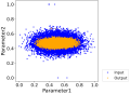
(a) Reconstruction result

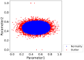
(b) Outlier detection result

Figure 2: Reconstruction result and outlier detection result for the dataset in Figure 1 when the loss function of the autoencoder is MSE-eig.

Similar to Section 3.1, we perform outlier detection on the same dataset in Figure 1 with our loss function. The reconstruction result and reconstruction error of any input value in each dimension is shown in Appendix B.2, which is consistent with our theoretical result of equation (3). Figure 2(a) shows the reconstruction result of the whole dataset. If the ratio of outliers is $0.05$, the HLP detected by the autoencoder are shown in Figure 2(b), we can intuitively see that all points with large Mahalanobis distance are detected as HLP, therefore, this result is consistent with the conclusion in Result 6. Besides, we also test the detection effect of our scheme for HLP with the dataset in Figure 1, see Appendix B.3. In particular, it can be seen clearly from Figure 11 in Appendix B.3 that MSE-trained autoencoders can’t detect HLP whose values in each dimension are within the normal range, and Figure 11 can reflect that most HLP with large Mahalanobis distance can be identified using our loss function.

4 Experiments

In this section, we will evaluate loss function MSE-eig on different datasets, low-dimensional synthetic datasets, high-dimensional synthetic datasets and a real dataset from International Mouse Phenotyping Consortium (IMPC). AUC (Area Under Curve) score is used to evaluate the accuracy of outlier detection results. Specifically, for the detection results of HLP, we compare our training loss function MSE-eig with MSE, and compute their AUC scores by regarding the HLP as positive. In addition, in order to reflect the detection effect of MSE-eig on IP, we compare the detection results of the autoencoder with the loss function MSE-eig, the autoencoder with the loss function MSE and the Mahalanobis distance for IP. In this case, IP are regarded as positive.

For each experiment, the structure of the autoencoder is as follows. The dimension of the hidden layer is the intrinsic dimension of the input dataset, and its activation function is RELU. Besieds, the activation function of the output layer is sigmoid. All datasets are normalized before outlier detection. During the autoencoder training process, Adam is used to optimize the loss function and the learning rate is $10^{-3}$. For our new training loss MSE-eig, we always set $\theta_{1}=0.008$ and $\theta_{2}=1$.

4.1 Synthetic data experiments

In this part, we test our method on both low-dimensional and high-dimensional datasets. Firstly, we generate a $3$D dataset whose intrinsic dimension is two. The dimensions represented by Parameter1 and Parameter3 follow 2-dimensional Gaussian distribution and the correlation coefficient between them is almost $0$. The value on the dimension represented by Parameter2 is equal to the square of the corresponding value on the dimension represented by Parameter1. We use this dataset as the training dataset (as shown in Figure 3(a)). It can be seen that the data points of the training dataset form a 2-dimensional manifold. Then, we generate the corresponding test set. The specific generation scheme is that based on the training set, we additionally generate some points that are not on the manifold of the training set, and these points are IP (as shown in Figure 3(b)). If the ratio of IP is $\delta_{1}$ and the number of sample points of the training dataset is $n$, we generate $\lfloor\delta_{1}n\rfloor$ data points that fall out of the manifold and consider these data points as positive. The corresponding AUC score of IP detection result is shown in Figure 4. We can see that although the detection effect of MSE-eig for IP is slightly worse than that of MSE, it is still significantly better than the detection effect based on Mahalanobis distance.

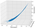
(a) Training dataset

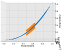
(b) Test dataset

Figure 3: Low-dimensional synthetic datasets, their actual dimension is 3 and intrinsic dimension is 2. (a) Training dataset, the value of Parameter2 is equal to the square of the value of Parameter1. (b) Test dataset, the correlation between the dimensions of the blue sample points is the same as the training dataset, while the correlation between the dimensions of the orange sample points is different from the training dataset.

As is known, in the $3$D training dataset generated above, HLP still exists. We also test the detection effect of MSE-eig on HLP in this training dataset. Since the dimensions represented by Parameter1 and Parameter3 obey 2-dimensional Gaussian distribution and the correlation coefficient between them is almost $0$, the values of the dimension represented by Parameter2 can be generated from the values of the dimension represented by Parameter1, for each data point, we only calculate its Mahalanobis distance based on parameter1 and parameter3. If the number of sample points of training dataset is $n$ and the ratio of HLP is $\delta_{2}$, we treat the top $\lfloor\delta_{2}n\rfloor$ points in Mahalanobis distance as positive. Figure 4 indicates that the detection effect of MSE-eig for HLP is comparable to that of Mahalanobis distance, but significantly better than that of MSE.

In addition, we treat both HLP and IP as positive to test outlier detection effect of MSE-eig. In our experiment, we assume that the ratio of HLP and the ratio of IP are equal, i.e., $\delta_{1}=\delta_{2}$. Figure 4 shows that MSE-eig works best for anomaly detection. In conclusion, MSE has the best detection effect for IP, but the detection effect for HLP is very poor. Conversely, Mahalanobis distance has the best detection results for HLP, but the detection effect for IP is the worst. However, MSE-eig can detect both very well.

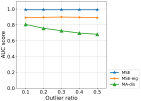
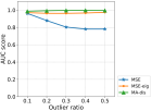
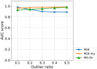
Figure 4: AUC scores for outlier detection results for the datasets in Figure 3 when the loss function of the autoencoder is MSE, MSE-eig or directly based on Mahalanobis distance. (a) Comparison result when IP present in the test dataset and only IP are considered as positive. (b) Comparison result when IP are not present in the test dataset and only HLP are considered as positive. (c) Comparison result when IP exist in the test dataset and both IP and HLP are considered as positive. We assume the same ratio of IP and HLP.

Then, we generate three different datasets with $2$D Gaussian distribution whose intrinsic dimension are also $2$ to evaluate our scheme. We find that MSE-eig outperforms MSE in detecting HLP in all three datasets at any outlier ratio. The specific results can be found in Appendix E.1. Besides, since autoencoders are often used for outlier detection in high-dimensional datasets, we also analyse the outlier detection results of MSE-eig on two high-dimensional synthetic datasets. MSE-eig is still better than MSE for HLP detection, see Appendix E.2 for details.

4.2 Real data experiments

IMPC is committed to phenotypic analysis of $20000$ mouse mutants, so that we can further predict the causative genes of various human genetic diseases. We download the experimental data from the official website of IMPC, which record the data of various physiological indicators of each gene knockout mouse. In our experiment, we select the data of $2$ physiological indicators for outlier detection and the joint distribution of this $2$-dimensional dataset approximates a $2$-dimensional Gaussian distribution. Besides, the training dataset has $6640$ sample points, and the test dataset has $15699$ sample points (as shown in Figures 5(a) and 5(b) respectively). The two physiological indicators we observe are Calcium and Total protein. It’s easy to see that outliers in these datasets are all HLP. Then we test the effectiveness of MSE-eig on the selected IMPC datasets and the corresponding result is presented in Figure 5(c). In real datasets, MSE-eig also outperforms MSE in outlier detection. This shows that our solution has extremely high application value.

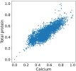
(a) Training dataset

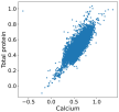
(b) Test dataset

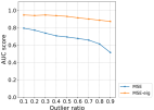
(c) Comparison result

Figure 5: IMPC datasets for outlier detection and AUC scores that reflect the outlier detection efficiency of MSE and MSE-eig.

5 Conclusion and future work

In this paper, we analyze the deficiencies of MSE-trained autoencoders for HLP detection. Through theoretical analysis, we demonstrate that properly suppressing complete reconstruction of the autoencoder is beneficial to improve the detection effect of HLP. Besides, we propose a new training loss function which can suppress complete reconstruction of the autoencoder during the training process to convert HLP into IP. Therefore, the outliers detected by our scheme cover both HLP and IP. Finally, we test our outlier detection scheme on both synthetic and real datasets and confirm the superiority of our approach.

It should be pointed out that there are still some interesting reseach directions that deserve further study. In the process of theoretical analysis, we assume that the dataset follows a multidimensional Gaussian distribution. However, for datasets that do not conform to a multidimensional Gaussian distribution, we would like to know how to obtain a scheme that controls their complete reconstruction through theoretical analysis. Besides, we are also curious about how to get the most reasonable value of $\beta$ through rigorous theoretical derivation.

Acknowledgments

This study is supported by the National Key Research and Development Program of China (2018YFA0801103), the National Natural Science Foundation of China (12071330) to Prof. Ling Yang. The authors would like to thank Professor Yu Tang (School of Mathematical Sciences, Soochow University) and Professor Huanfei Ma (School of Mathematical Sciences, Soochow University) for their valuable suggestions.

Appendix A More theoretical analysis for the importance of suppressing complete reconstruction

In this section, we will offer more detailed proofs for Result 1 and Result 2.

A.1 Proof of Result 1

Proof.

Let $\nu=\big{(}\nu_{1},\nu_{2},\ldots,\nu_{m}\big{)}^{\top}$ and $\Sigma_{Y}$ represent the mean vector and covariance matrix of variable $Y$ respectively, we have $\nu$ $=$ $P^{\top}\mu$ and $\nu_{k}$ $=$ $E(Y_{k})$ $=$ $\eta_{k}^{\top}\mu$, $k$ $=$ $1,2,\ldots,m$. Furthermore, we can gain the variance of the $k^{th}$ element of variable $Y$ is

$$\begin{split}D(Y_{k})&=COV\big{(}Y_{k},Y_{k}\big{)}\\ &=E\Big{(}\big{(}Y_{k}-\nu_{k}\big{)}\big{(}Y_{k}-\nu_{k}\big{)}\Big{)}\\ &=E\Big{(}\eta_{k}^{\top}\big{(}X-E(X)\big{)}\eta_{k}^{\top}\big{(}X-E(X)\big{)}\Big{)}\\ &=\eta_{k}^{\top}E\Big{(}\big{(}X-E(X)\big{)}\big{(}X-E(X)\big{)}^{\top}\Big{)}\eta_{k}\\ &=\eta_{k}^{\top}\Sigma_{x}\eta_{k}\\ &=\eta_{k}^{\top}\lambda_{k}\eta_{k}\\ &=\lambda_{k},\end{split}$$ (6)

and the covariance of $Y_{i}$ and $Y_{j}$ ($i$ $\neq$ $j$) is

$$\begin{split}COV(Y_{i},Y_{j})&=E\Big{(}\big{(}Y_{i}-E(Y_{i})\big{)}\big{(}Y_{j}-E(Y_{j})\big{)}\Big{)}\\ &=E\Big{(}\eta_{i}^{\top}\big{(}X-E(X)\big{)}\eta_{j}^{\top}\big{(}X-E(X)\big{)}\Big{)}\\ &=\eta_{i}^{\top}E\Big{(}\big{(}X-E(X)\big{)}\big{(}X-E(X)\big{)}^{\top}\Big{)}\eta_{j}\\ &=\eta_{i}^{\top}\Sigma_{x}\eta_{j}\\ &=\eta_{i}^{\top}\lambda_{j}\eta_{j}\\ &=0.\end{split}$$ (7)

Thus, the covariance matrix of variable $Y$ is $\Sigma_{Y}={\rm diag}(\lambda_{1},\lambda_{2},\ldots,\lambda_{m})$. ∎

A.2 Proof of Result 2

Proof.

As we know, the loss functhion of MSE can be formulated as

$$\begin{split}L_{MSE}(\omega,b)&=\frac{1}{n}\sum_{i=1}^{n}(y_{i}-\hat{y}_{i})^{\top}(y_{i}-\hat{y}_{i})\\ &=E\big{(}Y^{\top}Y-2Y^{\top}\hat{Y}+\hat{Y}^{\top}\hat{Y}\big{)}\\ &=E\big{(}Y^{\top}Y\big{)}-2E\big{(}Y^{\top}\hat{Y}\big{)}+E\big{(}\hat{Y}^{\top}\hat{Y}\big{)}\\ &=\sum_{i=1}^{m}E\big{(}Y_{i}^{2}\big{)}-2\sum_{i=1}^{m}E\big{(}Y_{i}\hat{Y}_{i}\big{)}+\sum_{i=1}^{m}E\big{(}\hat{Y}_{i}^{2}\big{)},\\ \end{split}$$ (8)

where $y_{i}$ and $\hat{y}_{i}$ represent the $i^{th}$ sample point of the input and output dataset in the new coordinate system respectively.

First, if the autoencoder can properly reconstruct the input dataset, we will analyse the mean vector of the output variable $\hat{Y}$. Based on Assumption 2 and equation (8), we have

$$\begin{split}L_{MSE}(\omega,b)&=\sum_{i=1}^{m}\lambda_{i}+\sum_{i=1}^{m}\hat{\lambda}_{i}+\sum_{i=1}^{m}\nu_{i}^{2}+\sum_{i=1}^{m}\hat{\nu}_{i}^{2}-2\sum_{i=1}^{m}\nu_{i}\hat{\nu}_{i}-2\sum_{i=1}^{m}COV\big{(}Y_{i},\hat{Y}_{i}\big{)}\\ &\geq\sum_{i=1}^{m}\big{(}\nu_{i}-\hat{\nu}_{i}\big{)}^{2}+\sum_{i=1}^{m}\Bigg{(}\sqrt{\lambda_{i}}-\sqrt{\hat{\lambda}_{i}}\Bigg{)}^{2}.\\ \end{split}$$ (9)

In order to reach the minima of $L_{MSE}(\omega,b)$, the mean vector of output variable $\hat{\nu}$ must satisfy $\hat{\nu}_{k}=\nu_{k}$, $k$ $=$ $1,2,\ldots,m$. That is to say, the mean vector of output data is the same as input data.

Next, we will specifically analyze the reconstruction error of each data point. According to Assumptions 1 and 2, the input and output variable satisfy $Y_{k}$ $\sim$ $\mathcal{N}(\nu_{k},\lambda_{k})$ and $\hat{Y}_{k}$ $\sim$ $\mathcal{N}(\nu_{k},\hat{\lambda}_{k})$, $k=1,2,\ldots,m$. Denote $R(Y)=\big{(}R_{1}(Y),R_{2}(Y),\ldots,R_{m}(Y)\big{)}^{\top}$ ($\hat{R}(Y)=\big{(}\hat{R}_{1}(Y),\hat{R}_{2}(Y),\ldots,\hat{R}_{m}(Y)\big{)}^{\top}$) as the difference between variable $Y$ ($\hat{Y}$) and its mean vector $\nu$, i.e., $R(Y)=Y-\nu$ and $\hat{R}(Y)=\hat{Y}-\nu$. It’s easy to see that $R_{k}(Y)$ $\sim$ $\mathcal{N}(0,\lambda_{k})$ and $\hat{R}_{k}(Y)$ $\sim$ $\mathcal{N}(0,\hat{\lambda}_{k})$. Then the following equation can be obtained.

$$\begin{split}L_{MSE}(\omega,b)&=E\Big{(}\big{(}Y-\hat{Y}\big{)}^{\top}\big{(}Y-\hat{Y}\big{)}\Big{)}\\ &=E\Big{(}\big{(}R(Y)-\hat{R}(Y)\big{)}^{\top}\big{(}R(Y)-\hat{R}(Y)\big{)}\Big{)}\\ &=E\Big{(}R^{\top}(Y)R(Y)\Big{)}-2E\Big{(}R^{\top}(Y)\hat{R}(Y)\Big{)}+E\Big{(}\hat{R}^{\top}(Y)\hat{R}(Y)\Big{)}\\ &=\sum_{i=1}^{m}E\Big{(}R_{i}^{2}(Y)\Big{)}+\sum_{i=1}^{m}E\Big{(}\hat{R}_{i}^{2}(Y)\Big{)}-2\sum_{i=1}^{m}E\Big{(}R_{i}(Y)\Big{)}E\Big{(}\hat{R}_{i}(Y)\Big{)}\\ &\hskip 14.22636pt-2\sum_{i=1}^{m}COV\Big{(}R_{i}(Y),\hat{R}_{i}(Y)\Big{)}\\ &=\sum_{i=1}^{m}\lambda_{i}+\sum_{i=1}^{m}\hat{\lambda}_{i}-2\sum_{i=1}^{m}\rho_{i}\sqrt{\lambda_{i}}\sqrt{\hat{\lambda}_{i}},\end{split}$$ (10)

where $\rho_{k}$ represents the correlation coefficient of $R_{k}(Y)$ and $\hat{R}_{k}(Y)$, and $-1\leq\rho_{k}\leq 1$, $k=1,2,\ldots,m$. In equation (10), only when $\rho_{k}=1$, can $L_{MSE}(\omega,b)$ reach its minima. In this case, there is a positive linear correlation between $R_{k}(Y)$ and $\hat{R}_{k}(Y)$, specifically, there exist constants $a_{k}$ and $c_{k}$ such that $\hat{R}_{k}(Y)=a_{k}R_{k}(Y)+c_{k}$, then $E\big{(}\hat{R}_{k}(Y)\big{)}=a_{k}E\big{(}R_{k}(Y)\big{)}+c_{k}$ and $D\big{(}\hat{R}_{k}(Y)\big{)}=a_{k}^{2}D\big{(}R_{k}(Y)\big{)}$. Since $E\big{(}\hat{R}_{k}(Y)\big{)}=E\big{(}R_{k}(Y)\big{)}=0$, $D\big{(}R_{k}(Y)\big{)}=\lambda_{k}$ and $D\big{(}\hat{R}_{k}(Y)\big{)}=\hat{\lambda}_{k}$, we can obtain $c_{k}=0$ and $a_{k}=\frac{\sqrt{\hat{\lambda}_{k}}}{\sqrt{\lambda_{k}}}$. Therefore, equation (1) is proved. ∎

Appendix B Reconstruction and outlier detection results

In this section, we provide more material showing the reconstruction results of MSE and MSE-eig for the datasets in Figures 1 and 1.

B.1 Reconstruction results of the MSE-trained autoencoder for the dataset in Figure 1

Figures 6(a) and 6(b) show the relationship between the reconstruction values and the corresponding input values in each dimension. For Parameter1 and Parameter2, we can see that reconstruction value increases monotonically with its corresponding input value. When the input values are between $0.15$ and $0.85$, they can be reconstructed well and the reconstructed values are approximately equal to the corresponding input values. Otherwise, if the values are very large or very small, the differences between the reconstructed values and the input values will be large and the corresponding reconstructed errors are large (as shown in Figures 6(c) and 6(d)). This confirms the correctness of our conclusions in Section 3.1.

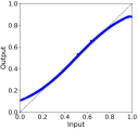
(a) Reconstruction result of parameter1

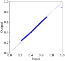
(b) Reconstruction result of parameter2

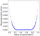
(c) Reconstruction error of parameter1

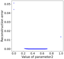
(d) Reconstruction error of parameter2

Figure 6: Reconstruction errors and reconstruction results for the dataset in Figure 1 when the loss function of the autoencoder is MSE. (a) and (b) present the reconstruction results of the values in each dimension. (c) and (d) show the reconstruction errors of the values in each dimension.

B.2 Reconstruction results of MSE-eig for the dataset in Figure 1

We perform outlier detection on the same dataset in Figure 1 with MSE-eig. By calculation, we get $\max(0.3\sqrt{\lambda_{1}},0.3\sqrt{\lambda_{2}})=0.05$, $\min(\sqrt{\lambda_{1}},\sqrt{\lambda_{2}})=0.13$ and the mean vector of this dataset is $(0.51,0.58)^{\top}$. So we set the hyperparameter $\beta=0.05$ in our loss function. Figures 7(a) and 7(b) show that for each dimension, all the input values can’t be well reconstructed. Figures 7(c) and 7(d) specifically show that the reconstruction error of any input value in each dimension is proportional to the square of the distance of the value from the mean, which is consistent with our theoretical analysis in Result 6.

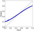
(a) Reconstruction result of parameter1

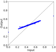
(b) Reconstruction result of parameter2

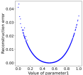
(c) Reconstruction error of parameter1

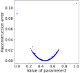
(d) Reconstruction error of parameter2

Figure 7: Reconstruction results and reconstruction errors for the dataset in Figure 1 when the loss function of the autoencoder is MSE-eig. (a) and (b) present the reconstruction results of the values in each dimension. (c) and (d) show the reconstruction errors of the values in each dimension.

B.3 Reconstruction results for the dataset in Figure 1

By calculation, for dataset in Figure 1, we get $\max(0.3\sqrt{\lambda_{1}},0.3\sqrt{\lambda_{2}})=0.04$ and $\min(\sqrt{\lambda_{1}},\sqrt{\lambda_{2}})=0.12$. Therefore, when using MSE-eig, we set $\beta=0.04$. Figures 8 and 9 present the reconstruction results of MSE and MSE-eig respectively, and Figure 10 show the reconstruction result of MSE-eig for the whole dataset and the corresponding outlier detection result. Figure 11 show the distribution of reconstruction errors for the whole dataset.

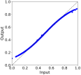
(a) Reconstruction result of parameter1

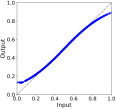
(b) Reconstruction result of parameter2

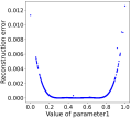
(c) Reconstruction error of parameter1

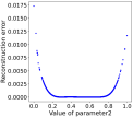
(d) Reconstruction error of parameter2

Figure 8: Reconstruction results and reconstruction errors for the dataset in Figure 1 when the loss function of the autoencoder is MSE. (a) and (b) present the reconstruction results of the values in each dimension. (c) and (d) show the reconstruction errors of the values in each dimension.

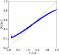
(a) Reconstruction result of parameter1

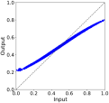
(b) Reconstruction result of parameter2

(c) Reconstruction error of parameter1

(d) Reconstruction error of parameter2

Figure 9: Reconstruction results and reconstruction errors for the dataset in Figure 1 when the loss function of the autoencoder is MSE-eig. (a) and (b) present the reconstruction results of the values in each dimension. (c) and (d) show the reconstruction errors of the values in each dimension.

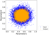
(a) Reconstruction result

(b) Outlier detection result

Figure 10: Reconstruction result and outlier detection result for the dataset in Figure 1 when the loss function of the autoencoder is MSE-eig.

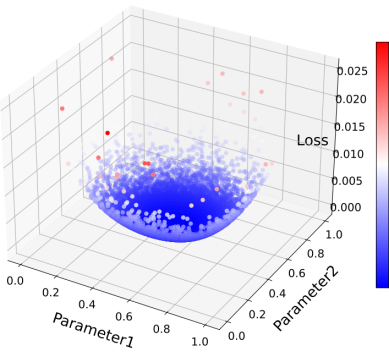
Figure 11: Reconstruction errors for the whole dataset in Figure 1 when the loss function of the autoencoder is MSE or MSE-eig. (a) When the loss function is MSE. (b) When the loss function is MSE-eig.

Appendix C Determination of hyperparameter $\beta$

If the intrinsic and actual dimensions of the dataset are equal, i.e., $l=m$, then most of the outliers in the dataset are HLP. In this case, considering that $\sqrt{\lambda_{k}}-\sqrt{\hat{\lambda}_{k}}>0$ and $\hat{\lambda}_{k}>0$, $k$ $=$ $1,2,\ldots,m$, Therefore, the value of the hyperparameter $\beta$ should satisfy $0<\beta<\mathop{\min}_{1\leq i\leq m}(\sqrt{\lambda_{i}})$. According to the previous analysis, as long as $\beta>0$, the detection effect of HLP can be improved. Meanwhile, in order to maintain the detection effect of IP, the value of $\beta$ must be small enough.

According to equation (1), if $\beta=0$, then $\hat{R}_{k}(Y)=R_{k}(Y)$, i.e., $\hat{Y}_{k}=Y_{k}$, $k$ $=$ $1,2,\ldots,m$. However, we will add nonlinear activation functions to the autoencoder to learn nonlinear features in the input dataset. For example, in our work, we add sigmoid activation function to the output layer. Since commonly used nonlinear activation functions are saturated, When the input values are very large or very small, the corresponding output values hardly change with the change of the input values. As the result, for each dimension of the input data, when the values are very large or very small, their reconstruction results are poor. Otherwise, the values can be reconstructed well. Then, most HLP detected by the autoencoder are anomalous in one dimension, but HLP whose values in each dimension are within the normal range are ignored. It can be seen from this that when $\beta$ is small enough, it not only adversely affects the detection effect of HLP, but also rarely improves the detection effect of IP. That is to say, there exists $\xi>0$, when $\beta<\xi$, there is not much improvement in the detection effect of IP.

If we determine the value of $\xi$ and let $\beta=\xi$, on the one hand, the detection effect of the autoencoder for IP can be maintained. On the other hand, we can suppress complete reconstruction of the autoencoder and avoid the influence of the saturation of the activation function on the data reconstruction at the same time, which can improve the detection effect for HLP.

In our work, the structure of the autoencoder and the setting of hyperparameters are described in Section 4. For each dimension of any dataset, input values between $0.15$ and $0.85$ are hardly affected by the saturation of the nonlinear activation function. Therefore, we hope that the value of $\beta$ selected can make the output value of each dimension between $0.15$ and $0.85$. As the result, for each dimension, the interval length of the output value is $0.7$ times the interval length of the input value. Before outlier detection, the input dataset is normalized, so the input value of each dimension is between $0$ and $1$. Recall that $Y_{k}$ $\sim$ $\mathcal{N}(\nu_{k},\lambda_{k})$ and $\hat{Y}_{k}$ $\sim$ $\mathcal{N}(\nu_{k},\hat{\lambda}_{k})$, $k=1,2,\ldots,m$, The probability that $Y_{k}$ is distributed in $(\nu_{k}-3\sqrt{\lambda_{k}},\nu_{k}+3\sqrt{\lambda_{k}})$ is $0.9974$, so its distribution interval length is approximately $6\sqrt{\lambda_{k}}$. Similarly, the distribution interval length of $\hat{Y}_{k}$ is approximately $6\sqrt{\hat{\lambda}_{k}}$. So we can control $\sqrt{\hat{\lambda}_{k}}=0.7\sqrt{\lambda_{k}}$, then $\sqrt{\lambda_{k}}-\sqrt{\hat{\lambda}_{k}}=0.3\sqrt{\lambda_{k}}$, $k=1,2,\ldots,m$.

Based on the above discussion, we can summarize how to determine the value of the hyperparameter $\beta$ when $l=m$. If $\mathop{\max}_{1\leq i\leq m}(0.3\sqrt{\lambda_{i}})\leq\mathop{\min}_{1\leq i\leq m}(\sqrt{\lambda_{i}})$, we can set $\beta=\mathop{\max}_{1\leq i\leq m}(0.3\sqrt{\lambda_{i}})$. Otherwise, we set $\beta=\mathop{\min}_{1\leq i\leq m}(\sqrt{\lambda_{i}})$.

In practical applications, we usually encounter this type of dataset whose intrinsic dimension $l$ is smaller than the actual dimension $m$. In this case, there are only $l$ eigenvalues of the covariance matrix of the dataset that are not close to $0$, we denote them as $\lambda^{{}^{\prime}}_{k}$, $k=1,2,\ldots,l$. In the training process, we only need to control such $l$ eigenvalues and make $\sqrt{\lambda^{{}^{\prime}}_{k}}-\sqrt{\hat{\lambda}^{{}^{\prime}}_{k}}=0.3\sqrt{\lambda^{{}^{\prime}}_{k}}$, $k=1,2,\ldots,l$. Besides, since $\lambda^{{}^{\prime}}_{k}>0$, $\beta$ should satisfy $0\leq\beta\leq\mathop{\min}_{1\leq i\leq l}(\sqrt{\lambda^{{}^{\prime}}_{i}})$. Actually, if $l<m$, there will be some data points that have a large impact on the reconstruction ability of the autoencoder (i.e., IP), it is very important to not only improve the detection effect of HLP, but also maintain the detection effect of IP. Therefore, we have to make sure that the value of $\beta$ is small enough but not equal to $0$. For convenience, we also set $0<\beta<\mathop{\min}_{1\leq i\leq m}(\sqrt{\lambda_{i}})$ in this case. Finally, the determination scheme for the value of $\beta$ is the same as when $l=m$.

Appendix D Training process of our outlier detection scheme

Algorithm 1 specifically describes the process of training the autoencoder with the improved loss function.

Input: Training dataset $\mathcal{D}$, hyperparameters $\theta_{1}$, $\theta_{2}$, $\beta$, and intrinsic dimension of training dataset $l$

Output: Outlier detection autoencoder with parameters $\omega$, $b$

foreach Epoch do

       foreach Batch $\mathcal{A}$ do

             if The dimension of the training dataset $m=l$ then

                   Calculate $\lambda_{i}$, $\hat{\lambda}_{i}$, $\i=1,\ldots,m$

                   Get $L_{MSE(\omega,b)}$ and $L_{EIG}(\omega,b)$

                   Updata the parameters $\omega$ and $b$ by minimizing $L_{MSE-eig}(\omega,b)$

             end if

            if The dimension of the training dataset $m>l$ then

                   Calculate $\lambda_{i}$, $\hat{\lambda}_{i}$, $\i=1,\ldots,m$

                   Select the $l$ eigenvalues $\lambda_{i}^{{}^{\prime}}$ that are not close to $0$ in the eigenvalues of the input dataset and their corresponding eigenvalues of the reconstruction result $\hat{\lambda}_{i}^{{}^{\prime}}$, $i=1,2,\ldots,l$

                   Get $L_{MSE(\omega,b)}$ and $L_{EIG}(\omega,b)$

                   Updata the parameters $\omega$ and $b$ by minimizing $L_{MSE-eig}(\omega,b)$

             end if

            

       end foreach

      

end foreach

Algorithm 1 Training process with MSE-eig

Appendix E More synthetic data experiments

In this section, we test the detection effect of MSE-eig on HLP on more synthetic datasets. In Section E.1, we conduct experiments on $3$ low-dimensional datasets. In Section E.2, experiments on $2$ high-dimensional datasets are provided.

E.1 Low-dimensional data experiments

We generate three datasets with $2$D Gaussian distribution, and their intrinsic dimension are also $2$. In one of the datasets, the correlation between the two dimensions is small (as shown in Figure 12(a)); the correlation between the two dimensions in another dataset is relatively large (as shown in Figure 12(b)); in the last dataset, the correlation between the two dimensions is also small and non-Gaussian distributed noise exist (as shown in Figure 12(c)). Obviously, the outliers in these three datasets are all HLP. Then we set different outlier ratios and calculate the corresponding AUC scores of the outlier detection results when the autoencoder uses MSE-eig and MSE as the loss function, respectively. To be specific, if the outlier ratio is $\delta$ and the number of sample points is $n$. Then the input data is sorted according to their Mahalanobis distance, and the first $\lfloor\delta n\rfloor$ sample points are regarded as positive. Figures 12(d), 12(e) and 12(f) show the test results on these three datasets. It’s easy to see that MSE-eig outperforms MSE in detecting HLP in all three datasets at any outlier ratio.

(a) Dataset1

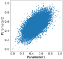
(b) Dataset2

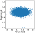
(c) Dataset3

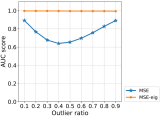
(d) AUC scores for Dataset1

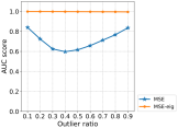
(e) AUC scores for Dataset2

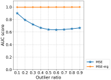
(f) AUC scores for Dataset3

Figure 12: Low-dimensional synthetic datasets and their outlier detection results. All datasets follow a two-dimensional Gaussian distribution. (a), (b) and (c) are data point distribution plots for each dataset. (a) Covariance matrix diagonal. (b) Covariance matrix off-diagonal. (c) Covariance matrix diagonal and non-Gaussian distributed noise exist. (d), (e) and (f) are AUC scores for outlier detection results for each dataset when the loss function of the autoencoder is MSE or MSE-eig. (d) Comparison result of Dataset1. (e) Comparison result of Dataset2. (f) Comparison result of Dataset3.

E.2 High-dimensional data experiments

Since autoencoders are often used for outlier detection in high-dimensional datasets, we also analyse the outlier detection result of MSE-eig on two high-dimensional synthetic datasets. Both datasets follow multidimensional Gaussian distribution and their covariance matrices are both diagonal matrices. So the intrinsic dimension of these two datasets are equal to their actual dimension. One of the datasets is $50$ dimensional and the other dataset is $100$ dimensional. It’s obvious that outliers in these two datasets are all HLP. Similar to Section E.1, we evaluate the outlier detection results of these two datasets by the AUC score, which are shown in Figure 13(a) and Figure 13(b) respectively. We can see that on high-dimensional datasets, MSE-eig is still better than MSE for HLP detection.

(a) 50-dimensional

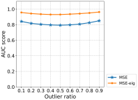
(b) 100-dimensional

Figure 13: AUC scores for outlier detection result for high-dimensional datasets when the loss function of the autoencoder is MSE or MSE-eig. Both datasets synthesized follow a multidimensional Gaussian distribution, and their covariance matrices are diagonal.

References

- Antwarg et al. (2021) Liat Antwarg, Ronnie Mindlin Miller, Bracha Shapira, and Lior Rokach. Explaining anomalies detected by autoencoders using shapley additive explanations. Expert Systems with Applications, 186:115736, 2021.
- Aoudi et al. (2018) Wissam Aoudi, Mikel Iturbe, and Magnus Almgren. Truth will out: Departure-based process-level detection of stealthy attacks on control systems. Proceedings of the 2018 ACM SIGSAC Conference on Computer and Communications Security, 2018.
- Bao et al. (2020) Xuchan Bao, James Lucas, Sushant Sachdeva, and Roger B. Grosse. Regularized linear autoencoders recover the principal components, eventually. CoRR, abs/2007.06731, 2020. URL http://dblp.uni-trier.de/db/journals/corr/corr2007.html#abs-2007-06731.
- Bergman & Hoshen (2020) Liron Bergman and Yedid Hoshen. Classification-based anomaly detection for general data. ArXiv, abs/2005.02359, 2020.
- Breunig et al. (2000) M. M. Breunig, H. P. Kriegel, R. T. Ng, and J. Sander. Lof: Identifying density-based local outliers. In Acm Sigmod International Conference on Management of Data, 2000.
- Chandola et al. (2009) Varun Chandola, Arindam Banerjee, and Vipin Kumar. Anomaly detection: A survey. ACM Comput. Surv., 41:15:1–15:58, 2009.
- Das et al. (2020) Tanmoy Kanti Das, Sridhar Adepu, and Jianying Zhou. Anomaly detection in industrial control systems using logical analysis of data. Comput. Secur., 96:101935, 2020.
- Gorokhov et al. (2017) O. Gorokhov, M. Petrovskiy, and I. Mashechkin. Convolutional neural networks for unsupervised anomaly detection in text data. Springer, Cham, 2017.
- Imon & Hadi (2013) A. H. M. Rahmatullah Imon and Ali S. Hadi. Identification of multiple high leverage points in logistic regression. Journal of Applied Statistics, 40:2601 – 2616, 2013.
- Kamoi & Kobayashi (2020) Ryo Kamoi and Kei Kobayashi. Why is the mahalanobis distance effective for anomaly detection? ArXiv, abs/2003.00402, 2020.
- Kim et al. (2020) K. H. Kim, S. Shim, Y. Lim, J. Jeon, J. Choi, B. Kim, and A. S. Yoon. Rapp: Novelty detection with reconstruction along projection pathway. In International Conference on Learning Representations, 2020.
- Lai et al. (2020) Chieh-Hsin Lai, Dongmian Zou, and Gilad Lerman. Robust subspace recovery layer for unsupervised anomaly detection. ArXiv, abs/1904.00152, 2020.
- Lin et al. (2018) Qin Lin, Sridhar Adepu, Sicco Verwer, and Aditya P. Mathur. Tabor: A graphical model-based approach for anomaly detection in industrial control systems. Proceedings of the 2018 on Asia Conference on Computer and Communications Security, 2018.
- Liu et al. (2008) Fei Tony Liu, Kai Ming Ting, and Zhi-Hua Zhou. Isolation forest. 2008 Eighth IEEE International Conference on Data Mining, pp. 413–422, 2008.
- Lu & Traore (2005) W. Lu and I. Traore. An unsupervised anomaly detection framework for network intrusions. 2005.
- Lyudchik (2016) O. R. Lyudchik. Outlier detection using autoencoders. 2016.
- MacDonald & Ghosh (2006) James W. MacDonald and Debashis Ghosh. Copa - cancer outlier profile analysis. Bioinformatics, 22 23:2950–1, 2006.
- Mahapatra et al. (2012) Amogh Mahapatra, Nisheeth Srivastava, and Jaideep Srivastava. Contextual anomaly detection in text data. Algorithms, 5:469–489, 2012.
- Nami & Shajari (2018) Sanaz Nami and Mehdi Shajari. Cost-sensitive payment card fraud detection based on dynamic random forest and k-nearest neighbors. Expert Syst. Appl., 110:381–392, 2018.
- Ning et al. (2022) Jin Ning, Leiting Chen, Chuan Zhou, and Yang Wen. Deep active autoencoders for outlier detection. Neural Processing Letters, 54(2):1399–1411, 2022.
- Oftadeh et al. (2020) Reza Oftadeh, Jiayi Shen, Zhangyang Wang, and Dylan Shell. Eliminating the invariance on the loss landscape of linear autoencoders. In International Conference on Machine Learning, pp. 7405–7413. PMLR, 2020.
- Ramaswamy et al. (2000) S. Ramaswamy, R. Rastogi, K. Shim, and T. Korea. Efficient algorithms for mining outliers from large data sets. In International Conference on Management of Data, 2000.
- Schlegl et al. (2017) Thomas Schlegl, Philipp Seeböck, Sebastian M. Waldstein, Ursula Margarethe Schmidt-Erfurth, and Georg Langs. Unsupervised anomaly detection with generative adversarial networks to guide marker discovery. In IPMI, 2017.
- Shetta & Niranjan (2020) O. Shetta and M. Niranjan. Robust subspace methods for outlier detection in genomic data circumvents the curse of dimensionality. Royal Society Open Science, 7(2):190714, 2020.
- Shyu et al. (2003) M. Shyu, S. Chen, K. Sarinnapakorn, and L Chang. A novel anomaly detection scheme based on principal component classifier. In Proc Icdm Foundation & New Direction of Data Mining Workshop, 2003.
- Sivakumar & Balasubramanian (2016) Nikita Sivakumar and R. Balasubramanian. Enhanced anomaly detection in imbalanced credit card transactions using hybrid pso. International Journal of Computer Applications, 135:28–32, 2016.
- Tibshirani & Hastie (2007) Robert Tibshirani and Trevor J. Hastie. Outlier sums for differential gene expression analysis. Biostatistics, 8 1:2–8, 2007.
- Zenati et al. (2018) Houssam Zenati, Chuan-Sheng Foo, Bruno Lecouat, Gaurav Manek, and Vijay Ramaseshan Chandrasekhar. Efficient gan-based anomaly detection. ArXiv, abs/1802.06222, 2018.
- Zhou & Paffenroth (2017) Chong Zhou and Randy C. Paffenroth. Anomaly detection with robust deep autoencoders. In KDD, pp. 665–674. ACM, 2017. ISBN 978-1-4503-4887-4. URL http://dblp.uni-trier.de/db/conf/kdd/kdd2017.html#ZhouP17.