The correlational entropy production during the local relaxation in a many body system with Ising interactions

Abstract

Isolated quantum systems follow the unitary evolution, which guarantees the full many body state always keeps a constant entropy as its initial one. In comparison, the local subsystems exhibit relaxation behavior and evolve towards certain steady states, which is called the local relaxation. Here we consider the local dynamics of finite many body system with Ising interaction. In both strong and weak coupling situations, the local observables exhibit similar relaxation behavior as the macroscopic thermodynamics; due to the finite size effect, recurrence appears after a certain typical time. Especially, we find that the total correlation of this system approximately exhibits a monotonic increasing envelope in both strong and weak coupling cases, which corresponds to the irreversible entropy production in the standard macroscopic thermodynamics. Moreover, the possible maximum of such total correlation calculated under proper constraints also coincides well with the exact result of time dependent evolution.

1 Introduction

A macroscopic thermodynamic system always tends to relax to the thermal equilibrium state after a long enough time in spite of its initial state. However, it is also known that an isolated quantum system with a finite number of degrees of freedom (DoF) follows the unitary evolution. As a result, the full many body system always keeps a constant entropy as its initial state, which looks different from the above macroscopic relaxation behavior, unless certain specific averaging approaches are taken into consideration, e.g., based on time or random defect configurations [1, 2, 3, 4, 5, 6, 7].

On the other hand, when focusing on the local parts of a many body system, the local dynamics naturally manifests similar relaxation behavior as the macroscopic thermodynamics. Although the whole isolated system always follows the unitary evolution and keeps a constant entropy, the dynamics of a local site exhibits an oscillating decay behavior, which seems relaxing towards a certain steady state, thus this is called the local relaxation [8, 9, 10, 11]. For a finite system size, the local relaxation would come across a “recurrence” after a typical time: the well ordered oscillatory decay behavior suddenly appears “random” [8, 9, 10, 11, 12, 13]. With the increase of the system size, the recurrence appears much later, thus it does not show up in practice.

But the entropy of each local system cannot indicate the irreversible entropy production behavior either, since it increases and decreases from time to time. In comparison, it is found that the total correlation in the many body system [14, 15, 16, 17, 18, 7] could manifest the irreversible entropy production similar as the standard thermodynamics [19, 20, 21, 22, 18, 9]. In this paper, we study the dynamical behavior of the total correlation during the local relaxation in an $N$-body system with Ising interactions. In both strong and weak coupling regimes, which correspond to the two phases of the Ising model with distinct physical properties though, the system dynamics exhibits quite similar local relaxation and recurrence behaviors, except in the strong coupling case the system dynamics contains more violent fluctuations.

Especially, it turns out the evolution of the total correlation roughly exhibits a monotonic increasing behavior in both strong and weak coupling cases, and approaches towards a steady value during the local relaxation process, which is similar to the irreversible entropy increase in the standard thermodynamics [19, 20, 21, 22]. Moreover, with the help of the Lagrangian multipliers, we calculate the possible maximum of the total correlation may achieve under proper constraints determined by the initial state, and it turns out such correlation maximization coincides quite well with the exact numerical result obtained from time dependent evolution. In this sense, the correlational entropy production well corresponds to the irreversible entropy production in the standard thermodynamics. We also show that in most common physical conditions, the correlational entropy production could reduce to the standard entropy production based on the thermal entropy $\text{\dj}Q/T$.

The paper is arranged as follows. In Sec. 2 we study the dynamics of the Ising model. In Sec. 3 we analyze the recurrence behavior in the local dynamics with different coupling strengths. In Sec. 4 we show the dynamics of the total correlation in this system. In Sec. 5 we show the correlational entropy production could reduce to the entropy production in the standard thermodynamics. The conclusion is drawn in Sec. 6.

2 Dynamics in a many-body system with Ising interaction

Here we consider an isolated many body system, which contains $N$ two-level systems (TLSs) with the periodic boundary condition. The $N$ TLSs interact with the near neighbors via the Ising interaction, which is described by the Hamiltonian [23]:

$$\hat{H}=\sum_{n=0}^{N-1}\frac{\omega}{2}\,\hat{\sigma}_{n}^{z}+J\,\hat{\sigma}_{n}^{x}\hat{\sigma}_{n+1}^{x}:=\hat{H}_{0}+\hat{V}_{J}.$$ (1)

Here $\hat{\sigma}_{n}^{x,z}$ are two Pauli matrices, and $\hat{\sigma}_{n}^{z}:=|\mathrm{e}\rangle_{n}\langle\mathrm{e}|-|\mathrm{g}\rangle_{n}\langle\mathrm{g}|$, $\hat{\sigma}_{n}^{x}:=\hat{\sigma}_{n}^{+}+\hat{\sigma}_{n}^{-}$, with $\hat{\sigma}_{n}^{+}:=(\hat{\sigma}_{n}^{-})^{\dagger}=|\mathrm{e}\rangle_{n}\langle\mathrm{g}|$. Here $|\mathrm{e}\rangle_{n}$, $|\mathrm{g}\rangle_{n}$ are the excited and ground states of the $n$-th TLS. The on-site energies ($\omega\geq 0$) of all the $N$ sites are equal, and $J$ is the interaction strength.

By applying the Jordan-Wigner transform [23],

$$\hat{\sigma}_{n}^{z} =2\hat{d}_{n}^{\dagger}\hat{d}_{n}-1,\qquad\hat{\sigma}_{n}^{+}=\hat{d}_{n}^{\dagger}\,\prod_{i=0}^{n-1}\left(-\hat{\sigma}_{i}^{z}\right),$$

$$\hat{\sigma}_{n}^{x} =\left(\hat{d}_{n}+\hat{d}_{n}^{\dagger}\right)\,\prod_{i=0}^{n-1}\left(-\hat{\sigma}_{i}^{z}\right),$$ (2)

the above Hamiltonian becomes a fermionic one, $\hat{H}=\sum_{n}\,\omega\,\hat{d}_{n}^{\dagger}\hat{d}_{n}+J(\hat{d}_{n}^{\dagger}\hat{d}_{n+1}+\hat{d}_{n}^{\dagger}\hat{d}_{n+1}^{\dagger}+\text{h.c.})$. Further, under the Fourier transform $\hat{d}_{n}=\sum_{k}\,\hat{c}_{k}\,e^{-i\frac{2\pi}{N}kn}/\sqrt{N}$, with $k=-\frac{1}{2}(N-1),\ldots,0\ldots,\frac{1}{2}(N-1)$, the Hamiltonian (1) becomes $\hat{H}=\frac{1}{2}\sum\mathbf{c}_{k}^{\dagger}\cdot\mathbf{H}_{k}\cdot\mathbf{c}_{k}$, where $\mathbf{c}_{k}:=(\hat{c}_{k},\,\hat{c}_{-k}^{\dagger})^{T}$ and

$$\mathbf{H}_{k}=\left[\begin{array}[]{cc}\frac{1}{2}\omega+2J\cos\frac{2\pi}{N}k&i2J\sin\frac{2\pi}{N}k\\ -i2J\sin\frac{2\pi}{N}k&-\left(\frac{1}{2}\omega+2J\cos\frac{2\pi}{N}k\right)\end{array}\right].$$ (3)

Then the system Hamiltonian can be diagonalized as $\hat{H}=\sum_{k>0}\,\varepsilon_{k}\,\hat{\gamma}_{k}^{\dagger}\hat{\gamma}_{k}-\varepsilon_{k}\,\hat{\gamma}_{-k}\hat{\gamma}_{-k}^{\dagger}$, where $\hat{\gamma}_{k}:=\cos\theta_{k}\,\hat{c}_{k}+i\sin\theta_{k}\,\hat{c}_{-k}^{\dagger}$ is the Bogoliubov operator, and $\varepsilon_{k}$ is the eigen mode energy [23]

$$\varepsilon_{k}=\big{[}(\frac{1}{2}\omega+2J\cos\frac{2\pi}{N}k)^{2}+4J^{2}\sin^{2}\frac{2\pi}{N}k\big{]}^{\frac{1}{2}},$$

$$\tan 2\theta_{k}=\frac{2J\sin\frac{2\pi}{N}k}{\frac{1}{2}\omega+2J\cos\frac{2\pi}{N}k}.$$ (4)

Based on these results, now we could obtain the exact time-dependent evolution of this isolated system. We consider that the initial state of the system is $|\varPsi_{0}\rangle=|\mathrm{e},\mathrm{g},\mathrm{g},\ldots\rangle$, namely, site-0 starts from the excited state $|\mathrm{e}\rangle_{0}$, and all the other sites start from the ground state $|\mathrm{g}\rangle_{n}$. Here site-0 could be regarded as an open “system”, while all the other $(N-1)$ TLSs build up a finite “bath”.

By using the Jordan-Wigner transform (2), such an initial state also can be rewritten as $|\varPsi_{0}\rangle=\hat{d}_{n=0}^{\dagger}\,|\mathbf{0}\rangle$, where $|\mathbf{0}\rangle$ is the vacuum state of the fermion system. Then we obtain the system state $|\varPsi_{t}\rangle$ at an arbitrary time, which gives

$$|\varPsi_{t}\rangle =e^{-i\hat{H}t}\,\hat{d}_{0}^{\dagger}|\mathbf{0}\rangle=\sum_{n=0}^{N-1}\Phi_{n}^{(N)}(t)\ \hat{d}_{n}^{\dagger}|\mathbf{0}\rangle,$$ (5)

$$\Phi_{n}^{(N)}(t) :=\sum_{k}\frac{e^{-i\frac{2\pi}{N}kn}}{N}\left(\cos^{2}\theta_{k}e^{i\varepsilon_{k}t}+\sin^{2}\theta_{k}e^{-i\varepsilon_{k}t}\right).$$

Here we call $\Phi_{n}^{(N)}(t)$ as a coherence function.

In principle now all the observable expectations can be calculated from $|\varPsi_{t}\rangle$. With the help of $\Phi_{n}^{(N)}(t)$ and the Jordan-Wigner transform (2), the excitation probability $p_{n,\mathrm{e}}(t):=\langle\mathrm{e}|\rho_{n}(t)|\mathrm{e}\rangle_{n}$ of the reduced density state $\rho_{n}$ of each site-$n$ gives

$$p_{n,\mathrm{e}}(t)=\langle\varPsi_{t}|\hat{d}_{n}^{\dagger}\hat{d}_{n}|\varPsi_{t}\rangle=|\Phi_{n}^{(N)}(t)|^{2},$$ (6)

and the total excitation of all the $N$ sites is $\langle\hat{\text{{n}}}_{\mathrm{t}}\rangle=\sum_{n}\,|\Phi_{n}^{(N)}(t)|^{2}$. Besides, from Eqs. (2, 5) it can be verified that the non-diagonal terms of the density state ${}_{n}\langle\mathrm{e}|\rho_{n}(t)|\mathrm{g}\rangle_{n}$ of each site always keep zero during the evolution [24].

Notice that, when the coupling strength is quite weak ($J\ll\omega$), in the interaction picture of $\hat{H}_{0}=\frac{1}{2}\omega\sum\hat{\sigma}_{n}^{z}$, the interaction in the Hamiltonian (1) becomes

$$\hat{V}_{J}(t) =J\sum_{n}\left(\hat{\sigma}_{n}^{+}e^{i\omega t}+\hat{\sigma}_{n}^{-}e^{-i\omega t}\right)\left(\hat{\sigma}_{n+1}^{+}e^{i\omega t}+\hat{\sigma}_{n+1}^{-}e^{-i\omega t}\right)$$

$$\simeq J\sum_{n}\left(\hat{\sigma}_{n}^{+}\hat{\sigma}_{n+1}^{-}+\hat{\sigma}_{n}^{-}\hat{\sigma}_{n+1}^{+}\right),$$ (7)

where the oscillating terms with frequencies $2\omega$ are neglected due to the rotating-wave approximation (RWA). Returning back to the Schrödinger picture the Hamiltonian becomes

$$\hat{H}=\sum_{n=0}^{N-1}\frac{\omega}{2}\,\hat{\sigma}_{n}^{z}+J(\hat{\sigma}_{n}^{+}\hat{\sigma}_{n+1}^{-}+\hat{\sigma}_{n}^{-}\hat{\sigma}_{n+1}^{+}).$$ (8)

This is also known as the quantum XX model [23], which guarantees the total excitation ($\hat{\text{{n}}}_{\mathrm{t}}\sim\sum\hat{\sigma}_{n}^{z}$) is conserved, while the original Ising model does not. Therefore, the behavior of the system dynamics would be similar as the quantum XX model in the weak coupling regime [9], while they would exhibit significant differences when $J$ is strong. Such a comparison could be well seen in our numerical results below.

3 The recurrence in the local dynamics

Now the full evolution of the $N$-body state is obtained exactly [Eq. (5)]. Since the whole isolated system follows the unitary evolution, if we do not consider the average over time or random defect configurations, the full $N$-body state $|\varPsi_{t}\rangle$ would always keep a pure state during the evolution. Namely, indeed $|\varPsi_{t}\rangle$ is never approaching any canonical thermal state as $\rho_{\text{th}}\sim\exp(-\hat{H}/k_{\text{{b}}}T)$.

In contrast, if we focus on the states of each local site, we would see the local dynamics exhibits similar behavior as the relaxation in macroscopic thermodynamics [13, 8, 9]. In Fig. 1(a, d), we show the evolution of the excitation probability $p_{n=0,\mathrm{e}}(t)$ of site-0 in both the strong and weak coupling regimes. Before a certain typical time $t\apprle t_{\text{rec}}$ (the vertical dashed red lines in Fig. 1), they both exhibits an oscillating decay behavior, which is quite similar as the relaxation in macroscopic thermodynamics. Namely, within the observation time $t<t_{\text{rec}}$, the population of site-0 (the “system”) seems relaxing towards $p_{0,\mathrm{e}}\rightarrow 0$ as its steady state.

But the decaying behavior suddenly changes around $t\sim t_{\text{rec}}$, the excitation probability $p_{0,\mathrm{e}}(t)$ shows a sudden increase and then looks “random”. This was referred as a “recurrence” due to the finite size effect [8, 13]. With the increase of the system size $N$, the recurrence time $t_{\text{rec}}$ also increases linearly [Fig. 1(b, f)]. When $N\rightarrow\infty$, the recurrence time would also be postponed and approach infinity. Thus at a finite time $t\ll t_{\text{rec}}$, only the irreversible relaxation behavior can be observed in practice [8, 13].

Besides, in the relaxation region before the recurrence $t\apprle t_{\text{rec}}$, notice that the decaying profiles for different system size $N$ are almost same with each other [Fig. 1(b, f)]. That indicates, once $J,\,\omega$ are fixed, the relaxation speed of this system is also fixed, which does not depend on the system size $N$. For a larger system size $N$, the full diffusion over the whole many-body system would cost more time.

It is worth noting that, such recurrences appear in both strong and weak coupling regimes (Fig. 1). In the weak coupling regime $J\ll\omega$, the system does show a dynamics similar as the XX model (8) as mentioned above [8, 9, 13]. In the strong coupling regime, the system dynamics also exhibits local relaxation and recurrence behaviors as the weak coupling situation, but contains more high frequency oscillations. For different parameter settings in both weak and strong regimes, we find that the recurrence time can be evaluated as $t_{\text{rec}}\equiv N(J^{-2}+16\omega^{-2})^{\frac{1}{2}}/2$, which is estimated from $t_{\text{rec}}\sim 2\pi/\delta\varepsilon$, with $\delta\varepsilon$ as the largest gap of the mode energies $\{\varepsilon_{k}\}$ (appearing around $2\pi k/N\sim\pm\pi/2$).

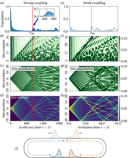
Figure 1: (a, e) The population evolution of site-$0$ $p_{0,\mathrm{e}}(t)=|\Phi_{0}^{(N=41)}(t)|^{2}$ in the strong ($\omega=0.1J$) and weak ($\omega=40J$) coupling regimes. (b, f) The scaling behavior of $p_{0,\mathrm{e}}(t)=|\Phi_{0}^{(N)}(t)|^{2}$ for different site numbers $N$. (c, g) The evolution of the local excitations $p_{n,\mathrm{e}}(t)$ of all the $N$ sites. (d, h) The evolution of the von Neumann entropy $S[\rho_{n}(t)]$ of all the $N$ sites. All the site numbers are set as $N=41$ except (b, f). (i) Demonstration for the propagation of the local excitations along the chain. Throughout this paper, we set $J=1$ as the energy unit, and all the evolutions are measured by the unitless time $\tau=Jt$.

In Fig. 1(c, g) we show the evolution of the excitation probabilities $p_{n,\mathrm{e}}(t)$ of all the $N$ sites. In both strong and weak coupling cases, we could clearly see a propagation process of the site excitations along the chain. Starting from site-0, the local excitations propagate along the two sides of the chain. For a finite system size, such propagations would meet each other at the periodic boundaries at $n\sim\pm N/2$, and then regathers back to site-0 again. This is just why the system exhibits its recurrence around $t\simeq t_{\text{rec}}$ [see the demonstrations in Fig. 1(i)]. After the recurrence, the system dynamics is combined with the regathered propagations together, thus appears more random. This propagation picture well explains why the recurrences appear in both the strong and weak coupling cases.

Indeed such propagation and regathering behaviors happen again and again, thus similar recurrence behavior could also appear around $t\simeq qt_{\text{rec}}$, with $q=1,2,3\ldots$ The system dynamics appears more and more “random” after each recurrence, and thus we call them hierarchy recurrences [9].

In Fig. 1(d, h) we show the evolution of the von Neumann entropy of each site, i.e., $S[\rho_{n}]\equiv-\mathrm{tr}[\rho_{n}\ln\rho_{n}]$. The entropy of each site increases and decreases from time to time, and also exhibit a propagation pattern along the chain in both both the strong and weak coupling situations. From this picture, we could see as long as there exist similar propagations of the local excitations, the local relaxations and such recurrences could appear in spite of the interaction strength and type.

4 Production of the total correlation

Now we see the local observables well exhibit the relaxation behaviors similar as the macroscopic thermodynamics, but the entropy of each site increases and decreases from time to time, which is different from the irreversible entropy production behavior in macroscopic thermodynamics. On the other hand, as an isolated system, the entropy of the whole system state always keeps the same as its initial state due to the the unitary evolution. Indeed, since the full $N$-body state here is not a canonical equilibrium state, the standard entropy production in macroscopic thermodynamics based on thermal entropy $dS=\text{\dj}Q/T$ cannot be applied here.

Notice that, in practical observations, the full $N$-body state is usually not directly assessable for local measurements, and it is the few-body observables that are directly measured [6, 22, 25]. Thus, here we consider the total correlation in this system, which is defined by [14, 15, 16, 17, 18, 7]

$$\mathbf{C}[\hat{\boldsymbol{\rho}}]:=\sum_{\alpha=0}^{N-1}S[\hat{\rho}_{\alpha}]-S[\hat{\boldsymbol{\rho}}].$$ (9)

Here $S[\hat{\boldsymbol{\rho}}]$ is the von Neumann entropy of the full $N$-body state $\hat{\boldsymbol{\rho}}$, which does not change during the unitary evolution, and $\hat{\rho}_{\alpha}$ are the reduced one-body states. This total correlation was firstly introduced for classical systems based on the collective probability distributions and the Shannon entropy [14], and the generalization for quantum systems by using density states and the von Neumann entropy is straightforward [15, 16, 17]. $\mathbf{C}[\hat{\boldsymbol{\rho}}]$ measures the total amount of all the correlations inside the $N$-body state $\hat{\boldsymbol{\rho}}$ [14, 15, 16, 17, 18, 7]. For $N=2$, the total correlation (9) just returns the mutual information in a two-body system, which measures the amount of the bipartite correlation.

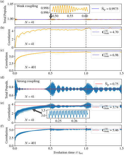
Figure 2: The evolution of the total excitation $\langle\hat{\text{{n}}}_{\mathrm{t}}\rangle$ (a, d), and the total correlation (b, c, e, f) in the weak (a-c, $\omega=40J$) and strong (d-f, $\omega=0.1J$) coupling regimes. The site numbers are set as $N=41$ in (a, b, d, e), while $N=401$ in (c, f). The dashed horizontal lines in (b, c, e, f) are the obtained by the total correlation maximization (14). The solid horizontal lines in (a, d) are $\tilde{\text{{n}}}_{\text{{p}}}\simeq 0.9975$ and $\tilde{\text{{n}}}_{\text{{p}}}\simeq 0.75$ respectively, which are the total excitations calculated by Eq. (11).

In Fig. 2(b, c, e, f), we show the time dependent evolution of the total correlation in both weak and strong coupling regimes, and they both exhibit an increasing behavior towards a steady value. In the weak coupling case [Fig. 2(b, c)], the behavior of the total correlation is similar as the XX model [9]. In the strong coupling case [Fig. 2(e, f)], the total correlation also exhibits an increasing envelope, but contains more violent oscillations. Moreover, with the increase of the system size $N$, the increasing curve in both cases become more and more smooth [Fig. 2(c, f)]. These behaviors are quite similar with the irreversible entropy production in the standard macroscopic thermodynamics.

In this sense, we further consider where is the destination that the total correlation is increasing towards. The possible maximum that $\mathbf{C}[\hat{\boldsymbol{\rho}}(t)]$ may achieve can be obtained by the variation approach under proper constraints [26].

Unlike the quantum XX model (8), here the total excitation of all the $N$ site is not conserved and changes with time. From the transformations (2, 4), the total excitation $\langle\hat{\text{{n}}}_{\mathrm{t}}\rangle=\sum_{n}\langle\hat{d}_{n}^{\dagger}(t)\hat{d}_{n}(t)\rangle$ gives

$$\langle\hat{\text{{n}}}_{\mathrm{t}}\rangle= \frac{1}{N}\sum_{k}\cos^{4}\theta_{k}-\left(i\sin\theta_{k}\cos\theta_{k}\right)^{2}e^{2i\varepsilon_{k}t}$$

$$-\left(i\sin\theta_{k}\cos\theta_{k}\right)^{2}e^{-2i\varepsilon_{k}t}+\sin^{4}\theta_{k}.$$ (10)

It turns out, in the weak coupling case [Fig. 2(a)], the total excitation exhibits quite small fluctuations with time around a certain constant, which is consistent with the above discussions about the reduction to the XX model by RWA. Thus, approximately the total excitation still could be treated as a variation constraint.

When the Ising interaction is strong [Fig. 2(d)], the total excitation exhibits significant fluctuations with time, which is quite different from the XX model. But it is also worth noting that, especially within the relaxation time $t\apprle t_{\text{rec}}/2$, the total excitation $\langle\hat{\text{{n}}}_{\mathrm{t}}\rangle$ seems converging towards a steady value, until a recurrence happens because of the finite size effect. Indeed the moment that the total excitation comes across its first recurrence ($\sim t_{\text{rec}}/2$) is just when the two-side propagations meet each other at the periodic boundaries at $n\sim\pm N/2$ [see Fig. 1(i)]. In the thermodynamic limit $N\rightarrow\infty$, recurrences do not appear, and the total excitation $\langle\hat{\text{{n}}}_{\mathrm{t}}\rangle$ is just relaxing to this steady value irreversibly.

Therefore, such a converging value of the total excitation $\langle\hat{\text{{n}}}_{\mathrm{t}}\rangle$ could be treated as an approximated constraint when we estimate the possible maximum where the total correlation is increasing towards. Further, since $\langle\hat{\text{{n}}}_{\mathrm{t}}\rangle$ keeps oscillating around a central value, this converging value can be estimated by the long time average of Eq. (10), which eliminates all the rotating terms, i.e., [27, 28, 29]

$$\tilde{\text{{n}}}_{\text{{p}}} :=\lim_{T\rightarrow\infty}\frac{1}{T}\int_{0}^{T}dt\,\langle\hat{\text{{n}}}_{\mathrm{t}}\rangle=\frac{1}{N}\sum_{k}\cos^{4}\theta_{k}+\sin^{4}\theta_{k}$$

$$= \frac{1}{2}+\frac{1}{2N}\sum_{k}\frac{(\frac{1}{2}\omega+2J\cos\frac{2\pi}{N}k)^{2}}{(\frac{1}{2}\omega+2J\cos\frac{2\pi}{N}k)^{2}+4J^{2}\sin^{2}\frac{2\pi}{N}k}.$$ (11)

In Fig. 2(a, d) we see $\tilde{\text{{n}}}_{\text{{p}}}$ does give the central value that $\langle\hat{\text{{n}}}_{\mathrm{t}}\rangle$ oscillates around [the horizontal solid lines].

In the thermodynamics limit $N\rightarrow\infty$, this central value becomes ($\tilde{J}\equiv J/\omega$)

$$\tilde{\text{{n}}}_{\text{{p}}}\stackrel{{\scriptstyle\text{{n}}\rightarrow\infty}}{{\longrightarrow}}\> \frac{1}{2}+\frac{1}{2}\int_{-\pi}^{\pi}\frac{dz}{2\pi}\,\frac{(\frac{1}{2}\omega+2J\cos z)^{2}}{(\frac{1}{2}\omega+2J\cos z)^{2}+4J^{2}\sin^{2}z}$$

$$= \begin{cases}3/4,&|\tilde{J}|\geq 1/2\\ 1-\tilde{J}^{2},&|\tilde{J}|<1/2\end{cases}.$$ (12)

$\tilde{\text{{n}}}_{\text{{p}}}(\tilde{J})$ has a singular point at $\tilde{J}\equiv J/\omega=1/2$, and this is just the critical point when discussing the ground state phase transition of the quantum Ising model.

In this sense, we adopt $\langle\hat{\text{{n}}}_{\mathrm{t}}\rangle\simeq\tilde{\text{{n}}}_{\text{{p}}}$ as an approximated constraint, and estimate the possible maximum of the total correlation by variation. As mentioned below Eq. (6), the density state $\rho_{n}$ of each site keeps diagonal during the evolution, thus its entropy is $S[\rho_{n}]=-p_{n,\mathrm{e}}\ln p_{n,\mathrm{e}}-p_{n,\mathrm{g}}\ln p_{n,\mathrm{g}}$ [$p_{n,\mathrm{g(e)}}$ is the probability that site-$n$ is in the ground (excited) state]. The full $N$-body state keeps a pure one, whose entropy is zero. With the help of Lagrangian multipliers, under the constraints (1) $p_{n,\mathrm{g}}+p_{n,\mathrm{e}}=1$, (2) $\langle\hat{\text{{n}}}_{\mathrm{t}}\rangle=\sum_{n}\,p_{n,\mathrm{e}}\simeq\tilde{\text{{n}}}_{\text{{p}}}$, the maximum of the total correlation $\mathbf{C}=\sum_{n}\,-p_{n,\mathrm{e}}\ln p_{n,\mathrm{e}}-p_{n,\mathrm{g}}\ln p_{n,\mathrm{g}}$ is calculated by taking variation of the functional

$$F\big{[}\{p_{n,\mathrm{e}}\},\lambda\big{]}:= \big{(}\sum_{n}-p_{n,\mathrm{e}}\ln p_{n,\mathrm{e}}-p_{n,\mathrm{g}}\ln p_{n,\mathrm{g}}\big{)}$$

$$+\lambda\big{(}\tilde{\text{{n}}}_{\text{{p}}}-\sum_{n}p_{n,\mathrm{e}}\big{)}$$ (13)

upon $p_{n,\mathrm{e}}$ and $\lambda$.

To look for the extremum, $\partial F/\partial p_{n,\mathrm{e}}\equiv 0=\ln(1-p_{n,\mathrm{e}})-\ln p_{n,\mathrm{e}}-\lambda$ indicates all $p_{n,\mathrm{e}}$ should be equal to each other. Thus the total correlation $\mathbf{C}[\{p_{n,\mathrm{e}}\}]$ achieves its possible maximum when all the $N$ sites take $p_{n,\mathrm{e}}=\tilde{\text{{n}}}_{\text{{p}}}/N$. As a result, the correlation maximization gives

$$\mathbf{C}_{\text{max}}^{(N)}=-\tilde{\text{{n}}}_{\text{{p}}}\ln\frac{\tilde{\text{{n}}}_{\text{{p}}}}{N}-(N-\tilde{\text{{n}}}_{\text{{p}}})\ln(1-\frac{\tilde{\text{{n}}}_{\text{{p}}}}{N}).$$ (14)

In the weak coupling regime [Fig. 2(b, c)] we see this correlation maximum (the dashed horizontal lines) is quite close to the time dependent result that the total correlation is increasing towards. In the strong coupling regime [Fig. 2(e, f)], though containing heavy oscillations, the envelope of the total correlation $\mathbf{C}(t)$ also coincide well with the possible maximum $\mathbf{C}_{\text{max}}^{(N)}$.

To make a more precise comparison, here we consider the coarse-grained total correlation, i.e.,

$$\tilde{\mathbf{C}}(t):=\frac{1}{2\Delta t}\int_{t-\Delta t}^{t+\Delta t}ds\,\mathbf{C}(s).$$ (15)

Namely, at time $t$, $\tilde{\mathbf{C}}(t)$ is a time average over a small period $2\Delta t$ in which many enough oscillations are included [30, 22]. In this sense $\tilde{\mathbf{C}}(t)$ gives the central line of the exact $\mathbf{C}(t)$ [the thick blue line in Fig. 3(a)], which turns out to be a smoothly increasing line. The maximum of $\tilde{\mathbf{C}}(t)$ appears around $t\simeq t_{\text{rec}}/2$, and we compare this $\text{max}\{\tilde{\mathbf{C}}(t)\}$ with the possible maximum $\mathbf{C}_{\text{max}}^{(N)}$. With the increase of the system size $N$, the relative error between $\text{max}\{\tilde{\mathbf{C}}(t)\}$ and $\mathbf{C}_{\text{max}}^{(N)}$ decreases [see Fig. 3(b)]. Thus, when the size $N\rightarrow\infty$, it is expectable that the coarse-grained total correlation $\tilde{\mathbf{C}}(t)$ is just increasing towards $\mathbf{C}_{\text{max}}^{(N)}$ as its destination.

Therefore, here the behavior of the total correlation in this system well manifests the irreversible entropy production in the standard macroscopic thermodynamics. Remember that the standard entropy production based on thermal entropy $dS=\text{\dj}Q/T$ cannot be applied for the nonequilibrium states here.

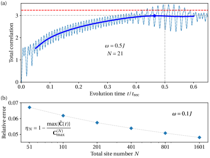
Figure 3: (a) Demonstration for the total correlation after coarse-graining (thick blue line, $\omega=0.1J$, $N=21$). The dash-dotted line is the original total correlation $\mathbf{C}(t)$ without coarse-graining. The dashed red line is the possible correlation maximum $\mathbf{C}_{\text{max}}^{(N)}$. (2) The relative error between $\mathbf{C}_{\text{max}}^{(N)}$ and the maximum of the coarse-grained correlation $\text{max}\big{\{}\tilde{\mathbf{C}}(t)\big{\}}$ around $t\simeq t_{\text{rec}}/2$ for different system sizes ($N=51,\,101,\,201,\,401,\,801,\,1601$, $\omega=0.1J$).

5 Reducing to entropy production in standard thermodynamics

Now we show that, under proper physical conditions, the total correlation could reduce to the entropy production in the standard thermodynamics.

In most open system problems, we consider an open system interacting with a bath, and the bath is usually modeled as a collection of many noninteracting DoFs $\hat{H}_{\textsc{b}}=\sum_{n}\hat{\textsc{h}}_{n}$, which is weakly coupled with the open system, and it is assumed that the initial state of the bath is a canonical thermal state $\hat{\rho}_{\text{{b}}}(0)\sim\exp(-\hat{H}_{\text{{b}}}/k_{\text{{b}}}T)$. When the system-bath interaction strength is negligibly small, since the bath is much larger than the open system, the bath state $\hat{\rho}_{\text{{b}}}(t)$ would not change too much comparing with its initial one, thus $\ln\hat{\rho}_{\text{{b}}}(t)\simeq\ln\hat{\rho}_{\text{{b}}}(0)+o[\delta\hat{\rho}_{\text{{b}}}(t)]$, and the changing rate of the bath entropy can be approximately obtained as [20, 31, 21, 32]

$$\dot{S}_{\text{{b}}}(t) =-\frac{d}{dt}\mathrm{tr}\left[\hat{\rho}_{\text{{b}}}(t)\ln\hat{\rho}_{\text{{b}}}(t)\right]=-\mathrm{tr}\big{[}\dot{\hat{\rho}}_{\text{{b}}}(t)\ln\hat{\rho}_{\text{{b}}}(t)\big{]}$$

$$\simeq-\mathrm{tr}\big{[}\dot{\hat{\rho}}_{\text{{b}}}(t)\ln\hat{\rho}_{\text{{b}}}(0)\big{]}=\frac{1}{T}\frac{d}{dt}\langle\hat{H}_{\text{{b}}}\rangle.$$ (16)

Notice that here the bath energy increase $\frac{d}{dt}\langle\hat{H}_{\text{{b}}}\rangle$ is just equal to the system energy loss $-\dot{Q}$, namely, the informational entropy change $\dot{S}_{\text{{b}}}$ could reduce to the thermal entropy (up to a minus sign), $dS_{\text{{b}}}=-\text{\dj}Q/T$. On the other hand, under the weak interactions, the different DoFs in the bath would not generate significant correlations during the evolution, thus approximately the bath entropy is just the summation of the entropy of each DoF, $S_{\text{{b}}}(t)\simeq\sum_{n}\,S[\hat{\varrho}_{\text{{b}},n}(t)]$, where $\hat{\varrho}_{\text{{b}},n}$ is the reduced density state of a certain DoF in the bath. Further, the open system plus the bath as a whole isolated system follows the unitary evolution, thus the entropy $S_{\text{{sb}}}$ of the full system does not change with time. Thus, the changing rate of the total correlation gives

$$\frac{d}{dt}\mathbf{C}=\frac{d}{dt}(S_{\text{{s}}}+S_{\text{{b}}}-S_{\text{{sb}}})\simeq\frac{d}{dt}S_{\text{{s}}}-\frac{1}{T}\frac{dQ}{dt}\geq 0,$$ (17)

which returns the irreversible entropy production in the standard thermodynamics [20, 21, 22]. In this sense, the second law statement that the irreversible entropy keeps increasing could be equivalently understood as the increase of total correlation in this whole system [33, 20, 34, 35, 36, 1, 37, 38, 39]. If the correlation between the different DoF inside the bath is significant, corrections should be considered [40].

Another analogy with the standard thermodynamics is the Boltzmann entropy increase in an isolated classical gas composed of $N$ particles with weak collisions. Since the full ensemble state $\rho(\vec{P},\vec{Q})$ of the N-body system follows the Liouville theorem, its Gibbs entropy [19, 22],

$$S_{\textsc{g}}[\rho(\vec{P},\vec{Q})]=-\int d^{3N}pd^{3N}q\,\rho\ln\rho,$$ (18)

never changes with time. One the other hand, the dynamics of the single particle probability distribution function (PDF) $\varrho_{n}(\mathbf{p}_{n},\mathbf{x}_{n})$ can be described by the Boltzmann equation. According to the Boltzmann H theorem [41], because of the particle collisions the PDF $\varrho_{n}(\mathbf{p}_{n},\mathbf{x}_{n})$ of each single particle always approaches the Maxwell-Boltzmann distribution ($\sim\exp[-E(\mathbf{p}_{n},\mathbf{x}_{n})/k_{\text{{b}}}T]$) as the steady state, with its entropy increasing monotonically. Notice that the single-particle PDF $\varrho_{n}(\mathbf{p}_{n},\mathbf{x}_{n})$ is a marginal distribution of the full ensemble state $\rho(\vec{P},\vec{Q})$, which is obtained by averaging out all the other particles. In this case the total correlation of the $N$ particle gas is

$$\mathbf{C}=\sum_{n}S_{\textsc{g}}[\varrho_{n}(\mathbf{p}_{n},\mathbf{x}_{n})]-S_{\textsc{g}}[\rho(\vec{P},\vec{Q})],$$ (19)

which sums up the entropy of all the $N$ single particle PDF, and $S_{\textsc{g}}[\rho(\vec{P},\vec{Q})]$ always keeps a constant during the evolution. Therefore, it turns out the increase of the total correlation $\delta\mathbf{C}(t)$ is just equal to the total Boltzmann entropy increase of the $N$ particle gas. Therefore, the total correlation reduces to the entropy production in the standard thermodynamics [19, 22, 42, 43].

In practice, usually it is the partial information (e.g., marginal distribution, few-body observable expectations) that is directly accessible to our observation. Indeed most macroscopic thermodynamic quantities are obtained only from such partial information like the one-body distribution, which exhibits irreversible behaviors. In practical measurements, the dynamics of the full many body state is quite difficult to be measured directly. In this sense, the reversibility of microscopic dynamics and the macroscopic irreversibility coincide with each other.

6 Conclusion

Here we consider the nonequilibrium dynamics in an isolated $N$-body system with Ising interaction. During the unitary evolution, without applying time average, the full $N$-body state always keeps a constant entropy, and the entropy of each single site increases and decreases from time to time. In comparison, the dynamics of the local observables exhibit local relaxation behavior, which is similar as the macroscopic thermodynamics. Due to the finite system size, recurrences appears in the local relaxations which roots from the superposition with the propagation regathered back. The total correlation approximately exhibits a monotonic increasing behavior, which is similar to the irreversible entropy increase in the standard thermodynamics. Even for the strong coupling situation where the total excitation has violent fluctuations, the total excitation exhibits an explicit converging behavior until the recurrence happens.We also show that in most common physical conditions, the correlational entropy production could reduce to the standard entropy production based on the thermal entropy. In this sense, the correlational entropy production is a well generalization for the standard entropy production.

References

-
[1]
A. Hobson,
Irreversibility in
Simple Systems, Am. J. Phys. 34 (5) (1966) 411–416.
doi:10.1119/1.1973009.
URL http://aapt.scitation.org/doi/10.1119/1.1973009 -
[2]
I. Prigogine, Time,
Structure, and Fluctuations, Science 201 (4358) (1978) 777–785.
doi:10.1126/science.201.4358.777.
URL http://science.sciencemag.org/content/201/4358/777 -
[3]
M. C. Mackey, The
dynamic origin of increasing entropy, Rev. Mod. Phys. 61 (4) (1989)
981–1015.
doi:10.1103/RevModPhys.61.981.
URL https://link.aps.org/doi/10.1103/RevModPhys.61.981 -
[4]
D. J. Evans, D. J. Searles,
The
Fluctuation Theorem, Adv. Phys. 51 (7) (2002) 1529–1585.
doi:10.1080/00018730210155133.
URL http://www.tandfonline.com/doi/abs/10.1080/00018730210155133 -
[5]
J. Uffink, Compendium of the
foundations of classical statistical physics, in: Philosophy of Physics,
Handbook of the Philosophy of Science, North Holland, Amsterdam, 2006, p.
923.
URL http://philsci-archive.pitt.edu/2691/ -
[6]
R. H. Swendsen,
Explaining
irreversibility, Am. J. Phys. 76 (7) (2008) 643–648.
doi:10.1119/1.2894523.
URL https://aapt.scitation.org/doi/10.1119/1.2894523 -
[7]
G. T. Landi, M. Paternostro,
Irreversible
entropy production: From classical to quantum, Rev. Mod. Phys. 93 (3)
(2021) 035008.
doi:10.1103/RevModPhys.93.035008.
URL https://link.aps.org/doi/10.1103/RevModPhys.93.035008 -
[8]
M. Cramer, C. M. Dawson, J. Eisert, T. J. Osborne,
Exact
Relaxation in a Class of Nonequilibrium Quantum Lattice Systems,
Phys. Rev. Lett. 100 (3) (2008) 030602.
doi:10.1103/PhysRevLett.100.030602.
URL http://link.aps.org/doi/10.1103/PhysRevLett.100.030602 -
[9]
S.-W. Li, C. P. Sun,
Hierarchy
recurrences in local relaxation, Phys. Rev. A 103 (4) (2021) 042201.
doi:10.1103/PhysRevA.103.042201.
URL https://link.aps.org/doi/10.1103/PhysRevA.103.042201 -
[10]
A. Flesch, M. Cramer, I. P. McCulloch, U. Schollwöck, J. Eisert,
Probing local
relaxation of cold atoms in optical superlattices, Phys. Rev. A 78 (3)
(2008) 033608.
doi:10.1103/PhysRevA.78.033608.
URL https://link.aps.org/doi/10.1103/PhysRevA.78.033608 -
[11]
J. Eisert, M. Friesdorf, C. Gogolin,
Quantum
many-body systems out of equilibrium, Nature Phys. 11 (2) (2015) 124–130.
doi:10.1038/nphys3215.
URL http://www.nature.com/nphys/journal/v11/n2/full/nphys3215.html -
[12]
P. Hänggi, P. Talkner, M. Borkovec,
Reaction-rate
theory: fifty years after Kramers, Rev. Mod. Phys. 62 (2) (1990) 251–341.
doi:10.1103/RevModPhys.62.251.
URL http://link.aps.org/doi/10.1103/RevModPhys.62.251 - [13] R. Zwanzig, Nonequilibrium statistical mechanics, 1st Edition, Oxford University Press, Oxford, 2001.
-
[14]
S. Watanabe,
Information
theoretical analysis of multivariate correlation, IBM J. Res. Dev. 4 (1)
(1960) 66–82.
doi:10.1147/rd.41.0066.
URL http://dl.acm.org/citation.cfm?id=1661258.1661265 -
[15]
B. Groisman, S. Popescu, A. Winter,
Quantum,
classical, and total amount of correlations in a quantum state, Phys. Rev. A
72 (3) (2005) 032317.
doi:10.1103/PhysRevA.72.032317.
URL https://link.aps.org/doi/10.1103/PhysRevA.72.032317 -
[16]
D. L. Zhou,
Irreducible
Multiparty Correlations in Quantum States without Maximal Rank,
Phys. Rev. Lett. 101 (18) (2008) 180505.
doi:10.1103/PhysRevLett.101.180505.
URL https://link.aps.org/doi/10.1103/PhysRevLett.101.180505 -
[17]
J. Goold, C. Gogolin, S. R. Clark, J. Eisert, A. Scardicchio, A. Silva,
Total correlations
of the diagonal ensemble herald the many-body localization transition, Phys.
Rev. B 92 (18) (2015) 180202.
doi:10.1103/PhysRevB.92.180202.
URL https://link.aps.org/doi/10.1103/PhysRevB.92.180202 -
[18]
F. Anza, F. Pietracaprina, J. Goold,
Logarithmic
growth of local entropy and total correlations in many-body localized
dynamics, Quantum 4 (2020) 250.
doi:10.22331/q-2020-04-02-250.
URL https://quantum-journal.org/papers/q-2020-04-02-250/ -
[19]
J. L. Lebowitz,
Macroscopic
laws, microscopic dynamics, time’s arrow and Boltzmann’s entropy, Physica
A 194 (1-4) (1993) 1–27.
doi:10.1016/0378-4371(93)90336-3.
URL https://linkinghub.elsevier.com/retrieve/pii/0378437193903363 -
[20]
S.-W. Li, Production
rate of the system-bath mutual information, Phys. Rev. E 96 (1) (2017)
012139.
doi:10.1103/PhysRevE.96.012139.
URL https://link.aps.org/doi/10.1103/PhysRevE.96.012139 -
[21]
Y.-N. You, S.-W. Li,
Entropy dynamics
of a dephasing model in a squeezed thermal bath, Phys. Rev. A 97 (1) (2018)
012114.
doi:10.1103/PhysRevA.97.012114.
URL https://link.aps.org/doi/10.1103/PhysRevA.97.012114 -
[22]
S.-W. Li, The Correlation
Production in Thermodynamics, Entropy 21 (2) (2019) 111.
doi:10.3390/e21020111.
URL https://www.mdpi.com/1099-4300/21/2/111 - [23] S. Sachdev, Quantum phase transitions, 2nd Edition, Cambridge University Press, Cambridge ; New York, 2011.
-
[24]
N. Wu, P. Yang,
Exact one- and
two-site reduced dynamics in a finite-size quantum Ising ring after a
quench: A semianalytical approach, Phys. Rev. B 103 (17) (2021) 174428.
doi:10.1103/PhysRevB.103.174428.
URL https://link.aps.org/doi/10.1103/PhysRevB.103.174428 -
[25]
P. Strasberg, Entropy production as
change in observational entropy, arXiv:1906.09933 (Jun. 2019).
URL http://arxiv.org/abs/1906.09933 -
[26]
E. T. Jaynes,
Information Theory
and Statistical Mechanics, Phys. Rev. 106 (4) (1957) 620–630.
doi:10.1103/PhysRev.106.620.
URL https://link.aps.org/doi/10.1103/PhysRev.106.620 -
[27]
M. Srednicki, Chaos and
quantum thermalization, Phys. Rev. E 50 (2) (1994) 888–901.
doi:10.1103/PhysRevE.50.888.
URL http://link.aps.org/doi/10.1103/PhysRevE.50.888 -
[28]
M. Rigol, M. Srednicki,
Alternatives to
Eigenstate Thermalization, Phys. Rev. Lett. 108 (11) (2012) 110601.
doi:10.1103/PhysRevLett.108.110601.
URL http://link.aps.org/doi/10.1103/PhysRevLett.108.110601 -
[29]
A. Polkovnikov, K. Sengupta, A. Silva, M. Vengalattore,
Colloquium:
Nonequilibrium dynamics of closed interacting quantum systems, Rev. Mod.
Phys. 83 (3) (2011) 863–883.
doi:10.1103/RevModPhys.83.863.
URL http://link.aps.org/doi/10.1103/RevModPhys.83.863 -
[30]
J. W. Gibbs,
Elementary
Principles in Statistical Mechanics, C. Scribner’s sons, 1902.
URL http://archive.org/details/elementaryprinc00gibbgoog -
[31]
E. Aurell, R. Eichhorn,
On the von Neumann
entropy of a bath linearly coupled to a driven quantum system, New J. Phys.
17 (6) (2015) 065007.
doi:10.1088/1367-2630/17/6/065007.
URL http://stacks.iop.org/1367-2630/17/i=6/a=065007 -
[32]
G. Manzano, J. M. Horowitz, J. M. R. Parrondo,
Quantum
Fluctuation Theorems for Arbitrary Environments: Adiabatic and
Nonadiabatic Entropy Production, Phys. Rev. X 8 (3) (2018) 031037.
doi:10.1103/PhysRevX.8.031037.
URL https://link.aps.org/doi/10.1103/PhysRevX.8.031037 -
[33]
M. Esposito, K. Lindenberg, C. Van den Broeck,
Entropy production as
correlation between system and reservoir, New J. Phys. 12 (1) (2010) 013013.
doi:10.1088/1367-2630/12/1/013013.
URL http://stacks.iop.org/1367-2630/12/i=1/a=013013 -
[34]
G. Manzano, F. Galve, R. Zambrini, J. M. R. Parrondo,
Entropy production
and thermodynamic power of the squeezed thermal reservoir, Phys. Rev. E
93 (5) (2016) 052120.
doi:10.1103/PhysRevE.93.052120.
URL http://link.aps.org/doi/10.1103/PhysRevE.93.052120 -
[35]
S. Alipour, F. Benatti, F. Bakhshinezhad, M. Afsary, S. Marcantoni, A. T.
Rezakhani,
Correlations
in quantum thermodynamics: Heat, work, and entropy production, Sci. Rep. 6
(2016) 35568.
doi:10.1038/srep35568.
URL http://www.nature.com/srep/2016/161021/srep35568/full/srep35568.html -
[36]
L. Pucci, M. Esposito, L. Peliti,
Entropy production
in quantum Brownian motion, J. Stat. Mech. 2013 (04) (2013) P04005.
doi:10.1088/1742-5468/2013/04/P04005.
URL http://stacks.iop.org/1742-5468/2013/i=04/a=P04005 -
[37]
Q. Zhang, A
general information theoretical proof for the second law of thermodynamics,
Sci. China Ser. G 51 (7) (2008) 813–816.
doi:10.1007/s11433-008-0085-7.
URL https://link.springer.com/article/10.1007/s11433-008-0085-7 -
[38]
J. M. Horowitz, T. Sagawa,
Equivalent
Definitions of the Quantum Nonadiabatic Entropy Production, J.
Stat. Phys. 156 (1) (2014) 55–65.
doi:10.1007/s10955-014-0991-1.
URL http://link.springer.com/article/10.1007/s10955-014-0991-1 -
[39]
N. Kalogeropoulos,
Time
irreversibility from symplectic non-squeezing, Physica A 495 (2018)
202–210.
doi:10.1016/j.physa.2017.12.066.
URL http://www.sciencedirect.com/science/article/pii/S0378437117313092 -
[40]
K. Ptaszyński, M. Esposito,
Entropy
Production in Open Systems: The Predominant Role of
Intraenvironment Correlations, Phys. Rev. Lett. 123 (20) (2019) 200603.
doi:10.1103/PhysRevLett.123.200603.
URL https://link.aps.org/doi/10.1103/PhysRevLett.123.200603 - [41] L. Landau, E. Lifshitz, Statistical Physics, Part 1, Butterworth-Heinemann, Oxford, 1980.
-
[42]
E. T. Jaynes, Gibbs vs
Boltzmann Entropies, Am. J. Phys. 33 (5) (1965) 391–398.
doi:10.1119/1.1971557.
URL https://aapt.scitation.org/doi/10.1119/1.1971557 -
[43]
G. Chliamovitch, O. Malaspinas, B. Chopard,
Kinetic Theory beyond the
Stosszahlansatz, Entropy 19 (8) (2017) 381.
doi:10.3390/e19080381.
URL http://www.mdpi.com/1099-4300/19/8/381