Calibration Meets Explanation:
A Simple and Effective Approach for Model Confidence Estimates

Abstract

Calibration strengthens the trustworthiness of black-box models by producing better accurate confidence estimates on given examples. However, little is known about if model explanations can help confidence calibration. Intuitively, humans look at important features attributions and decide whether the model is trustworthy. Similarly, the explanations can tell us when the model may or may not know. Inspired by this, we propose a method named CME that leverages model explanations to make the model less confident with non-inductive attributions. The idea is that when the model is not highly confident, it is difficult to identify strong indications of any class, and the tokens accordingly do not have high attribution scores for any class and vice versa. We conduct extensive experiments on six datasets with two popular pre-trained language models in the in-domain and out-of-domain settings. The results show that CME improves calibration performance in all settings. The expected calibration errors are further reduced when combined with temperature scaling. Our findings highlight that model explanations can help calibrate posterior estimates.

1 Introduction

Accurate estimates of posterior probabilities are crucial for neural networks in various Natural Language Processing (NLP) tasks Guo et al. (2017); Lakshminarayanan et al. (2017). For example, it would be helpful for humans if the models deployed in practice abstain or interact when they cannot make a decision with high confidence Jiang et al. (2012). While Pre-trained Language Models (PLMs) have improved the performance of many NLP tasks Devlin et al. (2019); Liu et al. (2019), how to better avoid miscalibration is still an open research problem  Desai and Durrett (2020); Dan and Roth (2021).

Positive	a fast funny highly enjoyable movie.
Negative	It’s about following your dreams no matter what your parents think.

Table 1: Two motivating examples with highlight explanations Socher et al. (2013). The saturation of the colors signifies the magnitude. The confidence of the model should be easily recognized by looking at token attributions.

In this paper, we investigate if and how model explanations can help calibrate the model.

Explanation methods have attracted considerable research interest in recent years for revealing the internal reasoning processes behind models Sundararajan et al. (2017); Heo et al. (2018); Shrikumar et al. (2017). Token attribution scores generated by explanation methods represent the contribution to the prediction Atanasova et al. (2020). Intuitively, one can draw some insight for analyzing and debugging neural models from these scores if they are correctly attributed, as shown in Table 1. For example, when the model identifies a highly indicative pattern, the tokens involved would have high attribution scores for the predicted label and low attribution scores for other labels. Similarly, if the model has difficulty recognizing the inductive information of any class (i.e., the attribution scores are not high for any label), the model should not be highly confident. As such, the computed explanation of an instance could indicate the confidence of the model in its prediction to some extent.

Inspired by this, we propose a simple and effective method named CME that can be applied at training time and improve the performance of the confidence estimates. The estimated confidence measures how confident the model is for a specific example. Ideally, reasonable confidence estimates should have higher confidence for correctly classified examples resulting in higher attributions than incorrect ones. Hence, given an example pair during training with an inverse classification relationship, we regularize the classifier by comparing the wrong example’s attribution magnitude and the correct example’s attribution magnitude.

Our work is related to recent works on incorporating explanations into learning. Different from previous studies that leverage explanations to help users predict model decisions Hase and Bansal (2021) or improve the accuracy Rieger et al. (2020), we focus on answering the following question: are these explanations of black-box models useful for calibration? If so, how should we exploit the predictive power of these explanations? Considering the model may be uninterpretable due to the nature of neural networks and limitations of explanation method Ghorbani et al. (2019); Yeh et al. (2019), a calibrated model by CME at least can output the unbiased confidence. Moreover, we exploit intrinsic explanation during training, which does not require designing heuristics Ye and Durrett (2022) and additional data augmentation Park and Caragea (2022).

We conduct extensive experiments using BERT Devlin et al. (2019) and RoBERTa Liu et al. (2019) to show the efficacy of our approach on three natural language understanding tasks (i.e., natural language inference, paraphrase detection, and commonsense reasoning) under In-Domain (ID) and Out-of-Domain (OD) settings. CME achieves the lowest expected calibration error without accuracy drops compared with strong SOTA methods, e.g., Park and Caragea (2022). When combined with Temperature Scaling (TS) Guo et al. (2017), the expected calibration errors are further reduced as better calibrated posterior estimates under these two settings.

2 Method

2.1 Problem Formulation

A well-calibrated model is expected to output prediction confidence (e.g., the highest probability after softmax activation) comparable to or aligned with its task accuracy (i.e., empirical likelihood). For example, given 100 examples with the prediction confidence of 0.8 (or 80%), we expect that 80 examples will be correctly classified. Following Guo et al. (2017), we estimate the calibration error by empirical approximations. Specifically, we partition all examples into $K$ bins of equal size according to their prediction confidences. Formally, for any $p\in[\ell_{k},u_{k})$, we define the empirical calibration error as:

$$\hat{\mathcal{E}}_{k}=\frac{1}{|\mathcal{B}_{k}|}\Big{|}\sum_{i\in\mathcal{B}_{k}}\big{[}\mathbbm{1}(\hat{y}_{i}=y_{i})-\hat{p}_{i}\big{]}\Big{|},$$ (1)

where $y_{i}$, $\hat{y}_{i}$ and $\hat{p}_{i}$ are the true label, predicted label and confidence for $i$-th example, and $\mathcal{B}_{k}$ denotes the bin with prediction confidences bounded between $\ell_{k}$ and $u_{k}$. To evaluate the calibration error of classifiers, we further adopt a weighted average of the calibration errors of all bins as the Expected Calibration Error (ECE) (Naeini et al., 2015):

$$\textrm{ECE}=\sum_{k=1}^{K}\frac{|\mathcal{B}_{k}|}{n}\hat{\mathcal{E}}_{k},$$ (2)

where $n$ is the example number and lower is better. Note that the calibration goal is to minimize the calibration error without significantly sacrificing prediction accuracy.

2.2 Our Approach

Generally, text classification models are optimized by Maximum Likelihood Estimation (MLE), which minimizes the cross-entropy loss between the predicted and actual probability over $k$ different classes. To minimize the calibration error, we add a regularization term to the original cross-entropy loss as a multi-task setup.

Our intuition is that if the error of the model on example $i$ is more significant than its error on example $j$ (i.e., example $i$ is considered more difficult for the classifier), then the magnitude of attributions on example $i$ should not be greater than the magnitude of attributions on example $j$. Moreover, we penalize the magnitude of attributions with the model confidence Xin et al. (2021), as the high error examples also should not have high confidence. Compared to the prior post-calibration methods (e.g., temperature scaling learns a single parameter with a validation set to rescale all the logits), our method is more flexible and sufficient to calibrate the model during training.

Formally, given a training set $\mathcal{D}=$ $\{(\boldsymbol{x}_{1},y_{1})$$,\cdots,$$(\boldsymbol{x}_{n},y_{n})\}$ where $\boldsymbol{x}_{i}$ is the embeddings of input tokens and $y_{i}$ is the one-hot vector corresponding to its true label, an attribution of the golden label for input $\boldsymbol{x}_{i}$ is a vector $\boldsymbol{a}_{i}=(a_{i1},\cdots,a_{il})$, and $a_{ij}$ is defined as the attribution of $x_{ij}$ ($l$ is the length). Here, attention scores are taken as the self-attention weights induced from the start index to all other indices in the penultimate layer of the model; this excludes weights associated with any special tokens added. Then, the token attribution $a_{ij}$ is the normalized attention score Jain et al. (2020) scaled by the corresponding gradients $\nabla\alpha_{ij}=\frac{\partial\hat{y}}{\partial\alpha_{ij}}$ Serrano and Smith (2019). At last, our training minimizes the following loss:

$$\mathcal{L}_{CME}=\mathcal{L}_{classify}+\lambda\mathcal{L}_{calib},$$ (3)

where $\lambda$ is a weighted hyperparameter. The $L_{calib}$ is calculated as follows:

$$\mathcal{L}_{calib} =\sum_{1\leq i,j\leq n}\Psi_{i,j}\mathbbm{1}[e_{i}>e_{j}],$$ (4)

$$\Psi_{i,j} =\max[0,t(\boldsymbol{x}_{i})-t(\boldsymbol{x}_{j})]^{2},$$ (5)

$$t(\boldsymbol{x}_{i}) =\lVert{a_{ij}}\rVert_{2}*c_{i},$$ (6)

where $e_{i}$ and $e_{j}$ are the error of example $i$ and example $j$, the confidence $c_{i}$ is estimated by the max probability of output Hendrycks and Gimpel (2017), with the L2 aggregation. The products could be further scaled by $\sqrt{l}$. In practice, strictly computing $L_{calib}$ for all example pairs is computationally prohibitive. Alternatively, we only consider examples from the mini-batch (similar lengths) of the current epoch. In other words, we consider all pairs where $e_{i}$ = 1 and $e_{j}$ = 0 where $e$ is calculated by using zero-one error function. The comparisons of example pairs can also be calculated from more history after every epoch or by splitting examples into groups, and we leave it to future work.

Algorithm 1 Explanation-based Calibrated Training

Inputs : Train set $\mathcal{D}$, Number of epochs $T$, Learning rate $\eta$, Optimizer $G$.
Output: Calibrated Text Model $M$

1:Random Initialize ${\boldsymbol{\theta}}$.

2:for epoch $=1\ldots T$ do

3:     Split $\mathcal{D}$ into random mini-batches {$b$}.

4:     for a batch $b$ from $\mathcal{D}$ do

5:         Backward model $M$ for $\nabla_{{\boldsymbol{\theta}}}\mathcal{L}_{classify}({\boldsymbol{\theta}},\mathcal{Y})$.

6:         Calculate the attribution by scaled attention.

7:         Computes absolute value of attributions.

8:         Normalized it by applying Softmax function.

9:         Calculate $\mathcal{L}_{CME}$ by Eqn. 3, 4, 5, 6.

10:         Optimize the model parameters ${\boldsymbol{\theta}}$ by G:

11:              ${\boldsymbol{\theta}}\leftarrow{\boldsymbol{\theta}}-\eta\nabla_{{\boldsymbol{\theta}}}\mathcal{L}_{CME}({\boldsymbol{\theta}},\mathcal{Y})$.

12:     end for

13:end for

Full training details are shown in Algorithm 1. To compute the gradient w.r.t the learnable weight independently, we retain the computation graph in the first back-propagation of classification loss. The model explanations are dynamically produced during training and then used to update the model parameters, which can be easily applied to most off-the-shelf neural networks.

3 Experiment

Methods	In-Domain						Out-of-Domain
	SNLI		QQP		SWAG		MNLI		TPPDB		HellaSWAG
	OOTB	TS	OOTB	TS	OOTB	TS	OOTB	TS	OOTB	TS	OOTB	TS
BERT	$2.54$	$1.14$	$2.71$	$0.97$	$2.49$	$0.85$	$7.09$	$3.61$	$8.51$	$7.15$	$12.62$	$12.83$
BERT+LS	$7.12$	$8.37$	$6.33$	$8.16$	$10.01$	$10.89$	$3.74$	$4.05$	$6.30$	$5.78$	$5.73$	$5.34$
Manifold-mixup	$3.17$	$1.77$	$8.55$	$6.11$	$5.18$	$1.09$	$12.92$	$2.34$	$12.10$	$7.98$	$9.82$	$5.12$
Manifold-mixup+LS	$3.40$	$5.14$	$3.49$	$3.71$	$5.24$	$1.26$	$16.76$	$4.57$	$6.29$	$6.54$	$8.32$	$3.64$
Park and Caragea (2022)	${1.29}$	${0.77}$	$2.05$	$1.02$	${2.01}$	$0.81$	$2.73$	$3.50$	${5.69}$	${3.16}$	${5.49}$	${4.11}$
Park and Caragea (2022)+LS	$1.85$	$1.05$	$1.70$	$0.95$	$2.09$	${0.79}$	${\bf{2.26}}$	${1.70}$	${5.37}$	$3.54$	${\bf{4.26}}$	${3.28}$
CME (Ours)	$\bf{1.11}$	$\bf{0.64}$	$\bf{1.66}$	$\bf{0.70}$	$\bf{1.16}$	$\bf{0.69}$	$2.65$	$\bf{1.59}$	${7.77}$	$\bf{1.59}$	${11.64}$	${\bf{2.11}}$
CME+LS (Ours)	$6.92$	$2.16$	${6.53}$	${2.73}$	$8.83$	${0.71}$	${4.32}$	${3.34}$	${\bf{4.21}}$	$3.83$	${6.40}$	${2.91}$
Methods	In-Domain						Out-of-Domain
	SNLI		QQP		SWAG		MNLI		TPPDB		HellaSWAG
	OOTB	TS	OOTB	TS	OOTB	TS	OOTB	TS	OOTB	TS	OOTB	TS
RoBERTa	$1.93$	$0.84$	$2.33$	$0.88$	$1.76$	${0.76}$	$3.62$	${1.46}$	$9.55$	$7.86$	$11.93$	$11.22$
RoBERTa+LS	$6.38$	$8.70$	$6.11$	$8.69$	$8.81$	$11.40$	$4.50$	$5.93$	$8.91$	$5.31$	$2.14$	$2.23$
Manifold-mixup	$7.32$	$4.56$	$3.54$	$5.05$	$1.68$	$0.96$	$19.78$	$7.65$	$7.18$	$8.76$	$5.63$	$3.43$
Manifold-mixup+LS	$3.51$	$3.00$	$2.82$	$3.03$	$1.83$	$0.94$	$8.23$	$5.08$	$6.17$	$6.91$	$4.27$	$2.88$
Park and Caragea (2022)	$1.34$	${{{0.63}}}$	$2.47$	$1.41$	$1.24$	$1.03$	$1.41$	${1.18}$	${\bf{3.94}}$	${1.89}$	$2.40$	${2.08}$
Park and Caragea (2022)+LS	${{1.28}}$	$1.02$	${2.18}$	$\bf{0.84}$	${{\bf{1.12}}}$	$0.81$	${\bf{1.37}}$	$1.60$	${3.96}$	${2.67}$	${\bf{1.86}}$	${1.70}$
CME (Ours)	${\bf{0.84}}$	$\bf{0.61}$	${\bf{1.33}}$	${1.16}$	$1.24$	${\bf{0.69}}$	$1.57$	$\bf{1.01}$	${9.26}$	$\bf{1.71}$	$9.01$	$\bf{1.44}$
CME+LS (Ours)	$6.83$	$1.26$	$6.88$	$2.77$	${8.01}$	$0.97$	${3.98}$	$2.84$	${7.77}$	${7.14}$	${3.80}$	${2.32}$

Table 2: Expected calibration errors ($\downarrow$) of BERT-based (Top) and RoBERTa-based (Bottom) models. We report the average results with five different random seeds. The standard deviations are in the Appendix E. The baselines are vanilla BERT Desai and Durrett (2020), Manifold-mixup Verma et al. (2019) and Park and Caragea (2022).

3.1 Dataset

We conduct the experiments in three natural language understanding tasks under the in-domain/out-of-the-domain settings: SNLI Bowman et al. (2015)/MNLI Williams et al. (2018) (natural language inference), QQP Iyer et al. (2017)/TPPDB Lan et al. (2017) (paraphrase detection), and SWAG Zellers et al. (2018)/HellaSWAG Zellers et al. (2019) (commonsense reasoning). We describe all datasets in details in Appendix A.

3.2 Results

Following Desai and Durrett (2020), we consider two settings: out-of-the-box (OOTB) calibration (i.e., we directly evaluate off-the-shelf trained models) and post-hoc calibration - temperature scaling (TS) (i.e., we rescale logit vectors with a single temperature for all classes). And we also experiment with Label Smoothing (LS) Pereyra et al. (2017); Wang et al. (2020) compared to traditional MLE training. The models are trained on the ID training set for each task, and the performance is evaluated on the ID and OD test sets. Additionally, we present implementation details and case studies in the Appendix B and D.

Table 2 shows the comparison of experimental results (ECEs) on BERT and RoBERTa. First, for OOTB calibration, we find that CME achieves the lowest calibration errors in the ID datasets except for RoBERTa in SWAG. At the same time, training with LS (i.e., CME+LS) exhibits more improvements in the calibration compared with original models in the TPPDB and HellaSWAG datasets. However, in most cases, LS models largely increase calibration errors for ID datasets. We conjecture that LS may affect the smoothness of the gradient and thus produces poor calibrated results. Secondly, for post-hoc calibration, we observe that TS always fails to correct miscalibrations of models with LS (e.g., CME-TS 0.64 vs. CME+LS-TS 2.16 in SNLI) under ID and OD settings. Nevertheless, TS reduces the ECEs in the OD setting by a large margin (e.g., HellaSWAG BERT 11.64 $\to$ 2.11). Compared to baselines, CME consistently improves over different tasks on calibration reduction of BERT-based models. While we apply CME to a relatively larger model, models with TS may perform better. It indicates that our method can be complementary to these post-hoc calibration techniques.

Model	Dev Acc.		Test Acc.
	ID	OD	ID	OD
Natural Language Inference (SNLI/MNLI)
BERT-MLE	90.18	74.04	90.04	73.52
RoBERTa-MLE	91.20	79.17	91.23	78.79
BERT-CME	90.22$\pm 0.20$	74.17$\pm 0.86$	90.22$\pm 0.22$	73.81$\pm 0.73$
RoBERTa-CME	91.62$\pm 0.14$	79.61$\pm 0.31$	91.37$\pm 0.41$	79.45$\pm 0.27$
Paraphrase Detection (QQP/TPPDB)
BERT-MLE	90.22	86.02	90.27	87.63
RoBERTa-MLE	89.97	86.17	91.11	86.72
BERT-CME	90.08$\pm 0.45$	86.22$\pm 0.09$	90.52$\pm 0.39$	87.46$\pm 0.26$
RoBERTa-CME	90.23$\pm 0.30$	86.38$\pm 0.76$	91.05$\pm 0.27$	86.44$\pm 0.67$
Commonsense Reasoning (SWAG/HellaSWAG)
BERT-MLE	78.82	38.01	79.40	34.48
RoBERTa-MLE	81.85	59.03	82.45	41.68
BERT-CME	77.57$\pm 0.54$	33.22$\pm 0.73$	78.94$\pm 0.29$	34.75$\pm 0.69$
RoBERTa-CME	80.13$\pm 0.25$	42.01$\pm 0.51$	82.47$\pm 0.35$	41.92$\pm 0.38$

Table 3: Average accuracy of development set and test set results for ID and OD datasets using pre-trained models with five random seeds. The results of BERT and RoBERTa baselines are from Table 2 and Table 6 of Desai and Durrett (2020).

3.3 Analysis

Table 3 presents the accuracy of BERT and RoBERTa on the development sets and test sets of our datasets. Our models have comparable accuracy (even better) compared to fine-tuned counterparts. For example, RoBERTa-CME has better accuracy than RoBERTa in the test set of the MNLI dataset (79.45 vs. 78.79). Specifically, CME performs poorly on the development set of HellaSWAG but performs comparably to baselines on the test set.

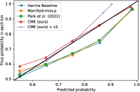
(a)

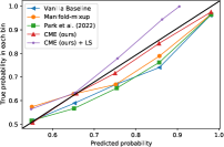
(b)

Figure 1: Visualization of calibration (OOTB) between different PLMs and competitive methods on QQP.

As shown in Figure 1, we visualize the alignment between the posterior probability measured by the model confidence and the empirical output measured by the accuracy. Note that a perfectly calibrated model has confidence equals accuracy for each bucket. Our model performs well under both PLMs architectures. We observe that, in general, CME helps calibrate the confidence of cases close to the decision boundary as it does not change most predictions. For example, compared to the baseline, CME optimizes the samples whose predicted probabilities are higher than actual probabilities. Moreover, we find that training with label smoothing technique can make the model underestimates some examples with high predicted probabilities. In addition, we conducted preliminary experiments with different batch sizes, and found that more large sizes did not significantly impact calibration performance. On the other hand, we found that larger LMs usually achieve both higher accuracy and better calibration performance (Table 2), which is in line with the observation in question answering Jiang et al. (2021).

4 Related Work

As accurate estimates are required for many difficult or sensitive prediction tasks Platt (1999), probability calibration is an important uncertainty estimation task for NLP. Unlike other uncertainty estimation task (e.g., out-of-domain detection, selective inference), calibration focuses on aleatoric uncertainty measured by the probability of the prediction and adjusts the overall model confidence level Hendrycks and Gimpel (2017); Pereyra et al. (2017); Guo et al. (2017); Qin et al. (2021). For example, Gal and Ghahramani (2016) propose to adopt multiple predictions with different dropout masks and then combine them to get the confidence estimate. Recently, several works focus on the calibration of PLMs models for NLP tasks Hendrycks et al. (2019); Desai and Durrett (2020); Jung et al. (2020); He et al. (2021); Park and Caragea (2022); Bose et al. (2022). Dan and Roth (2021) investigate the calibration properties of different transformer architectures and sizes of BERT. In line with recent work Ye and Durrett (2022), our work focuses on how explanations can help calibration in three NLP tasks. However, we do not need to learn a calibrator by using model interpretations with heuristics, and also do not compare due to its intensive computation cost when generating attributions. In contrast, we explore whether model explanations are useful for calibrating black-box models during training.

5 Conclusion

We propose a method that leverages model attributions to address calibration estimates of PLMs-based models. Considering model attributions as facts about model behaviors, we show that CME achieves the lowest ECEs under most settings for two popular PLMs.

6 Limitations

Calibrated confidence is essential in many high-stakes applications where incorrect predictions are highly problematic (e.g., self-driving cars, medical diagnoses). Though improving the performance on the calibration of pre-trained language models and achieving the comparable task performance, our explanation-based calibration method is still limited by the reliability and fidelity of interpretable methods. We adopt the scaled attention weight as the calculation method of attributions because (i) it has been shown to be more faithful in previous work Chrysostomou and Aletras (2022), and (ii) the interpretation of the model is that the internal parameters of the model participate in the calculation and are derivable. Despite the above limitations, it does not undermine the main contribution of this paper, as involving explanations when training helps calibrate black-box models. Our approach can apply to most NLP models, incurs no additional overhead when testing, and is modularly pluggable. Another promising research direction is to explore using free-text explanations to help calibrate the model.

Dataset	Class	Train/Dev/Test
SNLI Bowman et al. (2015)	3	549367 / 4921 / 4921
MNLI Williams et al. (2018)	3	391176 / 4772 / 4907
QQP Iyer et al. (2017)	2	363178 / 20207 / 20215
TPPDB Lan et al. (2017)	2	42200 / 4685 / 4649
SWAG Zellers et al. (2018)	4	73546 / 10003 / 10003
HellaSWAG Zellers et al. (2019)	4	39905 / 5021 / 5021

Table 4: Dataset statistics with number of classes and pre-processed train/development/test splits.

Dataset	Statistics	Train	Dev	Test
SNLI	Avg. Seq. Length	27.27	28.62	28.54
	Num. of class-0	183416	1680	1649
	Num. of class-1	183187	1627	1651
	Num. of class-2	182764	1614	1621
MNLI	Avg. Seq. Length	40.50	39.65	40.01
	Num. of class-0	130416	1736	1695
	Num. of class-1	130381	1535	1631
	Num. of class-2	130379	1501	1581
QQP	Avg. Seq. Length	31.00	30.92	31.06
	Num. of class-0	229037	12772	12768
	Num. of class-1	134141	7435	7447
TPPDB	Avg. Seq. Length	38.65	40.76	40.51
	Num. of class-0	31033	3744	3769
	Num. of class-1	11167	941	880
SWAG	Avg. Seq. Length	124.65	127.84	128.35
	Num. of class-0	18414	2453	2480
	Num. of class-1	18334	2500	2529
	Num. of class-2	18340	2546	2492
	Num. of class-3	18458	2504	2502
HellaSWAG	Avg. Seq. Length	338.84	347.64	347.64
	Num. of class-0	9986	1244	1271
	Num. of class-1	10031	1257	1228
	Num. of class-2	9867	1295	1289
	Num. of class-3	10021	1225	1233

Table 5: Average sequence lengths after tokenization and label distributions of datasets.

Appendix A Dataset Statistics

Table 4 and Table 5 present the characteristics of all datasets. The information across the three data splits includes the average sequence length and the number of examples under each label. Then we briefly introduce the datasets:

Natural Language Inference

The in-domain dataset is the Stanford Natural Language Inference (SNLI) dataset Bowman et al. (2015). It is used to predict if the relationship between the hypothesis and the premise (i.e., neutral, entailment and contradiction, ) for natural language inference task. The out-of-domain dataset is the Multi-Genre Natural Language Inference (MNLI) Williams et al. (2018), which covers more diverse domains compared with SNLI.

Paraphrase Detection

The in-domain dataset is the Quora Question Pairs (QQP) dataset Iyer et al. (2017). It is proposed to test if two questions are semantically equivalent as a paraphrase detection task. The out-of-domain dataset is the Twitter news URL Paraphrase Database (TPPDB) dataset Lan et al. (2017). It is used to determine whether Twitter sentence pairs have similar semantics when they share URL and we set the label less than 3 as the first class, and the others as the second class following previous works.

Commonsense Reasoning

The in-domain dataset is the Situations With Adversarial Generations (SWAG) dataset Zellers et al. (2018). It is a popular benchmark for commonsense reasoning task where the objective is to pick the most logical continuation of a statement from a list of four options. The out-of-domain dataset is the HellaSWAG dataset Zellers et al. (2019). It is generated by adversarial filtering and is more challenging for out-of-domain generalization.

Appendix B Experimental Settings

For all experiments, we report the average performance results of five random seed initializations for a maximum of 3 epochs. For a fair comparison, we follow most of the hyperparameters of Desai and Durrett (2020) unless reported below. For BERT, the batch size is 32 (SNLI/QQP) or 8 (SWAG) and the learning rate is $1\times 10^{-5}$, the weight of gradient clip is 1.0, and we exclude weight decay mechanism. For RoBERTa, the batch size is 16 (SNLI/QQP) or 8 (SWAG) and the learning rate is $2\times 10^{-5}$, the weight of gradient clip is 1.0, and the weight decay is 0.1. The maximum sequence length is set to 256. The optimal weights of $\lambda$ in Eqn. 3 are 0.05 and 1.0 for BERT and RoBERTa, respectively. We search the weight with respect to ECEs on the development sets from $[0.05,0.1,0.5,1.0]$. The hyperparameter of label smoothing $\sigma$ is 0.1. All experiments are conducted on NVIDIA Tesla A100 40G GPUs. We perform the temperature scaling searches in the range of [0.01,10.0] with a granularity of 0.01 using development sets. The search processes are fast as we use cached predicted logits of each dataset. The training time is moderate compared to the baseline. For example, on a A100 GPU, training the model with BERT and RoBERTa takes around 3-4 hours for QQP dataset. For the experiments in this paper, we use $K=10$.

Figure 2: Reliability diagram of ablation study. We train each BERT-based variant, and adopt QQP as the ID dataset which is relatively unbalanced in labels.

Appendix C Ablation Study

As shown in Figure 2, we find that using only confidence in Eqn. 6 generally yields higher ECE than other variants. Also using attention instead of scaled attention brings an increase in errors.

Appendix D Case Study

As shown in the Table 6, we list randomly-selected examples of BERT-base models with MLE and CME. If models correctly predict the true label, the model confidence should be greater than 50%. For example, in the second case of out-of-domain SNLI dataset, the model confidence of true label falls slightly below the borderline probability which results in an incorrect prediction (Probabilities: 30.54%, 30.83%, 38.63% vs. 67.87%, 14.66%, 17.47%). In contrast, CME leverages model explanation during training that helps calibrate the model confidence and predicts correctly.

Appendix E Standard Deviations

Table 7 lists the standard deviations of each methods. We report the results across five runs with random seeds.

Data	Input	True Label	MLE	CME
SNLI	Premise: The shadow silhouette of a woman standing near the water looking at a large attraction on the other side. Hypothesis: She is in the water.	contradiction	21.91	81.64
		Test#1544	wrong	correct
	Premise: A child is jumping off a platform into a pool. Hypothesis: The child is swimming.	entailment	30.54	67.87
		Test#1841	wrong	correct

MNLI	Premise: There are no means of destroying it; and he dare not keep it. Hypothesis: He should keep it with him.	contradiction	18.33	80.78
		Test#560	wrong	correct
	Premise: yeah that’s that’s a big step yeah Hypothesis: Yes, you have to be committed to make that big step.	neutral	49.43	69.18
		Test#1016	wrong	correct

SWAG	Prompt: Among them, someone embraces someone and someone. Someone Options: (A). is brought back to the trunk beside him. (B). waits for someone someone and the clerk at the dance wall. (C). scoops up someone and hugs someone. (D). looks at her, utterly miserable.	C	47.29	59.84
		Test#940	wrong	correct
	Prompt: He is holding a violin and string in his hands. He Options: (A). is playing an accordian on the stage. (B). talks about how to play it and a harmonica. (C). picks up a small curling tool and begins talking. (D). continues to play the guitar too.	B	32.32	45.00
		Test#30	correct	wrong

Table 6: Examples with model confidence of true label by MLE and CME in the SNLI/MNLI and SWAG dataset. The labels of SNLI/MNLI are entailment, contradiction and neutral. We list most cases with probabilities of true label that CME predicts correctly and the predictions of MLE are wrong.

Methods	In-Domain						Out-of-Domain
	SNLI		QQP		SWAG		MNLI		TPPDB		HellaSWAG
	OOTB	TS	OOTB	TS	OOTB	TS	OOTB	TS	OOTB	TS	OOTB	TS
BERT	$0.8$	$1.0$	$0.5$	$0.1$	$1.8$	$0.4$	$2.1$	$1.7$	$0.6$	$0.9$	$2.8$	$2.1$
BERT+LS	$0.3$	$0.5$	$0.4$	$0.7$	$1.0$	$1.1$	$1.4$	$0.9$	$0.8$	$0.7$	$0.6$	$0.9$
Manifold-mixup	$0.8$	$0.3$	$1.2$	$1.1$	$0.6$	$0.4$	$2.6$	$1.9$	$2.3$	$2.6$	$1.2$	$0.9$
Manifold-mixup+LS	$0.4$	$0.7$	$0.2$	$0.7$	$0.5$	$0.2$	$1.3$	$0.9$	$1.1$	$1.7$	$0.7$	$0.6$
Park and Caragea (2022)	${0.4}$	${0.7}$	$0.6$	$0.6$	${0.4}$	$0.2$	$2.5$	$0.6$	${0.7}$	${1.2}$	${1.9}$	${1.5}$
Park and Caragea (2022)+LS	$0.3$	$1.0$	$0.9$	$0.1$	$0.7$	${0.3}$	${{1.0}}$	${0.5}$	${1.0}$	$1.1$	${{0.8}}$	${0.7}$
CME (Ours)	${0.3}$	$0.2$	${0.5}$	${0.1}$	${0.2}$	${0.2}$	$0.3$	${0.6}$	${0.8}$	${0.2}$	${1.8}$	${{0.4}}$
CME+LS (Ours)	$0.3$	$0.2$	${0.1}$	${0.3}$	$1.5$	${0.2}$	${0.7}$	${1.0}$	${{1.5}}$	$0.6$	${1.8}$	${0.7}$
Methods	In-Domain						Out-of-Domain
	SNLI		QQP		SWAG		MNLI		TPPDB		HellaSWAG
	OOTB	TS	OOTB	TS	OOTB	TS	OOTB	TS	OOTB	TS	OOTB	TS
RoBERTa	$0.5$	$0.8$	$0.1$	$0.6$	$1.0$	${0.7}$	$3.2$	$2.5$	$0.6$	$0.5$	$3.2$	$2.9$
RoBERTa+LS	$0.6$	$1.0$	$0.3$	$0.6$	$0.3$	$0.6$	$1.4$	$1.9$	$0.3$	$0.7$	$1.4$	$1.1$
Manifold-mixup	$0.8$	$0.4$	$0.5$	$0.6$	$1.2$	$0.3$	$3.1$	$1.3$	$1.8$	$2.1$	$2.8$	$1.5$
Manifold-mixup+LS	$1.0$	$0.9$	$0.7$	$0.6$	$1.5$	$0.4$	$1.6$	$1.0$	$0.9$	$1.1$	$0.6$	$1.6$
Park and Caragea (2022)	$0.7$	${0.5}$	$0.6$	$0.2$	$0.1$	$0.2$	$1.9$	${1.4}$	${0.9}$	${1.2}$	$1.8$	$1.5$
Park and Caragea (2022)+LS	${0.6}$	$0.6$	${0.7}$	${0.4}$	${0.4}$	$0.1$	${1.7}$	$1.3$	${1.6}$	${1.8}$	${0.9}$	${1.2}$
CME (Ours)	$0.6$	${0.2}$	$0.5$	$0.1$	$1.0$	$0.2$	$0.8$	${0.3}$	${0.5}$	${0.8}$	$1.8$	$0.6$
CME+LS (Ours)	${0.4}$	$0.3$	${0.4}$	${0.2}$	${0.9}$	$0.2$	${0.6}$	$1.0$	${0.6}$	${0.4}$	${1.3}$	${1.6}$

Table 7: The standard deviations of BERT-based and RoBERTa-based models.

References

- Atanasova et al. (2020) Pepa Atanasova, Jakob Grue Simonsen, Christina Lioma, and Isabelle Augenstein. 2020. A diagnostic study of explainability techniques for text classification. In Proc. of EMNLP.
- Bose et al. (2022) Tulika Bose, Nikolaos Aletras, Irina Illina, and Dominique Fohr. 2022. Dynamically refined regularization for improving cross-corpora hate speech detection. In Proc. of ACL Findings.
- Bowman et al. (2015) Samuel R. Bowman, Gabor Angeli, Christopher Potts, and Christopher D. Manning. 2015. A Large Annotated Corpus for Learning Natural Language Inference. In Proc. of EMNLP.
- Chrysostomou and Aletras (2022) George Chrysostomou and Nikolaos Aletras. 2022. An empirical study on explanations in out-of-domain settings. In Proc. of ACL.
- Dan and Roth (2021) Soham Dan and Dan Roth. 2021. On the effects of transformer size on in- and out-of-domain calibration. In Proc. of EMNLP Findings.
- Desai and Durrett (2020) Shrey Desai and Greg Durrett. 2020. Calibration of pre-trained transformers. In Proc. of EMNLP.
- Devlin et al. (2019) Jacob Devlin, Ming-Wei Chang, Kenton Lee, and Kristina Toutanova. 2019. BERT: Pre-training of deep bidirectional transformers for language understanding. In Proc. of NAACL.
- Gal and Ghahramani (2016) Yarin Gal and Zoubin Ghahramani. 2016. Dropout as a bayesian approximation: Representing model uncertainty in deep learning. In Proc. of ICML.
- Ghorbani et al. (2019) Amirata Ghorbani, Abubakar Abid, and James Y. Zou. 2019. Interpretation of neural networks is fragile. In Proc. of AAAI.
- Guo et al. (2017) Chuan Guo, Geoff Pleiss, Yu Sun, and Kilian Q. Weinberger. 2017. On calibration of modern neural networks. In Proc. of ICML.
- Hase and Bansal (2021) Peter Hase and Mohit Bansal. 2021. When can models learn from explanations? A formal framework for understanding the roles of explanation data. arXiv preprint arXiv:2102.02201.
- He et al. (2021) Tianxing He, Bryan McCann, Caiming Xiong, and Ehsan Hosseini-Asl. 2021. Joint energy-based model training for better calibrated natural language understanding models. In Proc. of EACL.
- Hendrycks and Gimpel (2017) Dan Hendrycks and Kevin Gimpel. 2017. A baseline for detecting misclassified and out-of-distribution examples in neural networks. In Proc. of ICLR.
- Hendrycks et al. (2019) Dan Hendrycks, Kimin Lee, and Mantas Mazeika. 2019. Using pre-training can improve model robustness and uncertainty. In Proc. of ICML.
- Heo et al. (2018) Jay Heo, Haebeom Lee, Saehoon Kim, Juho Lee, Kwang Joon Kim, Eunho Yang, and Sung Ju Hwang. 2018. Uncertainty-aware attention for reliable interpretation and prediction. In Proc. of NeurIPS.
- Iyer et al. (2017) Shankar Iyer, Nikhil Dandekar, and Kornél Csernai. 2017. Quora Question Pairs.
- Jain et al. (2020) Sarthak Jain, Sarah Wiegreffe, Yuval Pinter, and Byron C. Wallace. 2020. Learning to faithfully rationalize by construction. In Proc. of ACL.
- Jiang et al. (2012) Xiaoqian Jiang, Melanie Osl, Jihoon Kim, and Lucila Ohno-Machado. 2012. Calibrating predictive model estimates to support personalized medicine. J. Am. Medical Informatics Assoc.
- Jiang et al. (2021) Zhengbao Jiang, Jun Araki, Haibo Ding, and Graham Neubig. 2021. How can we know When language models know? on the calibration of language models for question answering. Trans. Assoc. Comput. Linguistics, 9:962–977.
- Jung et al. (2020) Taehee Jung, Dongyeop Kang, Hua Cheng, Lucas Mentch, and Thomas Schaaf. 2020. Posterior calibrated training on sentence classification tasks. In Proc. of ACL.
- Lakshminarayanan et al. (2017) Balaji Lakshminarayanan, Alexander Pritzel, and Charles Blundell. 2017. Simple and scalable predictive uncertainty estimation using deep ensembles. In Proc. of NIPS.
- Lan et al. (2017) Wuwei Lan, Siyu Qiu, Hua He, and Wei Xu. 2017. A Continuously Growing Dataset of Sentential Paraphrases. In Proc. of EMNLP.
- Liu et al. (2019) Yinhan Liu, Myle Ott, Naman Goyal, Jingfei Du, Mandar Joshi, Danqi Chen, Omer Levy, Mike Lewis, Luke Zettlemoyer, and Veselin Stoyanov. 2019. Roberta: A robustly optimized bert pretraining approach. arXiv preprint arXiv:1907.11692.
- Naeini et al. (2015) Mahdi Pakdaman Naeini, Gregory F. Cooper, and Milos Hauskrecht. 2015. Obtaining well calibrated probabilities using bayesian binning. In Proc. of AAAI.
- Park and Caragea (2022) Seoyeon Park and Cornelia Caragea. 2022. On the calibration of pre-trained language models using mixup guided by area under the margin and saliency. In Proc. of ACL.
- Pereyra et al. (2017) Gabriel Pereyra, George Tucker, Jan Chorowski, Lukasz Kaiser, and Geoffrey E. Hinton. 2017. Regularizing neural networks by penalizing confident output distributions. In Proc. of ICLR.
- Platt (1999) John C. Platt. 1999. Probabilistic outputs for support vector machines and comparisons to regularized likelihood methods. In ADVANCES IN LARGE MARGIN CLASSIFIERS.
- Qin et al. (2021) Yao Qin, Xuezhi Wang, Alex Beutel, and Ed H. Chi. 2021. Improving calibration through the relationship with adversarial robustness. In Proc. of NeurIPS.
- Rieger et al. (2020) Laura Rieger, Chandan Singh, W. James Murdoch, and Bin Yu. 2020. Interpretations are useful: Penalizing explanations to align neural networks with prior knowledge. In Proc. of ICML.
- Serrano and Smith (2019) Sofia Serrano and Noah A. Smith. 2019. Is attention interpretable? In Proc. of ACL.
- Shrikumar et al. (2017) Avanti Shrikumar, Peyton Greenside, and Anshul Kundaje. 2017. Learning important features through propagating activation differences. In Proc. of ICML.
- Socher et al. (2013) Richard Socher, Alex Perelygin, Jean Wu, Jason Chuang, Christopher D. Manning, Andrew Y. Ng, and Christopher Potts. 2013. Recursive deep models for semantic compositionality over a sentiment treebank. In Proc. of EMNLP.
- Sundararajan et al. (2017) Mukund Sundararajan, Ankur Taly, and Qiqi Yan. 2017. Axiomatic attribution for deep networks. In Proc. of ICML.
- Verma et al. (2019) Vikas Verma, Alex Lamb, Christopher Beckham, Amir Najafi, Ioannis Mitliagkas, David Lopez-Paz, and Yoshua Bengio. 2019. Manifold mixup: Better representations by interpolating hidden states. In Proc. of ICML.
- Wang et al. (2020) Shuo Wang, Zhaopeng Tu, Shuming Shi, and Yang Liu. 2020. On the inference calibration of neural machine translation. In Proc. of ACL.
- Williams et al. (2018) Adina Williams, Nikita Nangia, and Samuel R. Bowman. 2018. A Broad-Coverage Challenge Corpus for Sentence Understanding through Inference. In Proc. of NAACL.
- Xin et al. (2021) Ji Xin, Raphael Tang, Yaoliang Yu, and Jimmy Lin. 2021. The art of abstention: Selective prediction and error regularization for natural language processing. In Proc. of ACL/IJCNLP.
- Ye and Durrett (2022) Xi Ye and Greg Durrett. 2022. Can explanations be useful for calibrating black box models? In Proc. of ACL.
- Yeh et al. (2019) Chih-Kuan Yeh, Cheng-Yu Hsieh, Arun Sai Suggala, David I. Inouye, and Pradeep Ravikumar. 2019. On the (in)fidelity and sensitivity of explanations. In Proc. of NeurIPS.
- Zellers et al. (2018) Rowan Zellers, Yonatan Bisk, Roy Schwartz, and Yejin Choi. 2018. SWAG: A Large-Scale Adversarial Dataset for Grounded Commonsense Inference. In Proc. of EMNLP.
- Zellers et al. (2019) Rowan Zellers, Ari Holtzman, Yonatan Bisk, Ali Farhadi, and Yejin Choi. 2019. HellaSWAG: Can a Machine Really Finish Your Sentence? In Proc. of ACL.