Automated Rendezvous & Docking Using 3D Vision

Abstract

The robustness and accuracy of a vision system for motion estimation of a tumbling target satellite are enhanced by an adaptive Kalman filter. This allows a vision-guided robot to complete the grasping of the target even if occlusion occurs during the operation. A complete dynamics model, including aspects of orbital mechanics, is incorporated for accurate estimation. Based on the model, an adaptive Kalman filter is developed that estimates not only the system states but also all the model parameters such as the inertia ratio, center-of-mass, and the rotation of the principal axes of the target satellite. An experiment is conducted by using a robotic arm to move a satellite mockup according to orbital mechanics while the satellite pose is measured by a laser camera system. The measurements are sent to the Kalman filter, which, in turn, drives another robotic arm to grasp the target. The results demonstrate successful grasping even if the vision system is blocked for several seconds.

1 Introduction

Internationally, there has been growing interest in using space robotic systems for the on-orbit servicing of spacecraft [1, 2, 3, 4, 5, 6, 7, 8, 9]. In such missions, the accurate motion estimation of a free-falling target spacecraft is essential for guiding a robotic arm so as to capture the target. Different vision systems are available for the estimation of the pose (position and orientation) of moving objects. Among them, an active vision system such as the Neptec Laser Camera system (LCS) is preferable for its robustness in face of the harsh lighting conditions of space [10]. As successfully verified during the STS-105 space mission, the 3D imaging technology used in LCS can indeed operate in space environment. The use of laser range data has also been proposed for the motion estimation of free-floating space objects [11, 12, 13, 14, 15, 16]. All vision systems, however, provide discrete and noisy pose data at relatively low rate, typically 1 Hz, while the capture of a free-falling object is a difficult robotic task which requires real-time and accurate pose estimation.

Taking advantage of the simple dynamics of a free-floating object, researchers have employed different observers to track and predict the motion of a target satellite [17, 11]. In some circumstances, e.g., when there are occlusions, no observation data is available. Therefore, long-term prediction of the motion of the object is needed for planning operations such as autonomous grasping of targets [17, 11].

The Kalman filter uses a dynamics model to compute a rough estimate of the system states, which is then corrected using a model of the sensor measurements to obtain the best estimate possible of the system states based on the present and past measurements. However, the applicability of the Kalman filtering technique rests on the accuracy of the dynamics and the measurement-noise models.

In this work, we use the Euler-Hill equations to derive a discrete-time model that captures the evolution of the relative translational motions of a tumbling target satellite with respect to a chaser satellite which is free-falling in a nearby orbit [18, 9]. Taking advantage of the structure of the model, we derive numerically efficient expressions for the state transition matrix and the covariance of the process noise, both of which are necessary for the Kalman filter. We also derive the sensitivity matrix of the observation and show that the observations of the translational and rotational displacements are coupled. Moreover, the kinematic properties of the unit-norm quaternions used to represent the relative orientation of the target satellite, is employed to derive the associated measurement-noise covariance. The new model allows additive quaternion noise while preserving the unit-norm property of the quaternion. This Kalman filter has been implemented in Matlab/Simulink and used in real-time to permit the autonomous capture of a tumbling satellite using a chaser arm. The performance of the Kalman filter is such that it is possible to fully occlude the vision system and perform the capture of the satellite more than 20 seconds after the occlusion using only the output of the EKF to provide a prediction of the pose of the satellite.

2 Modelling

2.1 Linearization

Figure 1 illustrates the chaser and the target satellites as rigid bodies moving in orbits nearby each other. Coordinate frames $\{A\}$ and $\{B\}$ are attached to the chaser and the target, respectively. The origin of $\{B\}$ is located at the target centre of mass (CM) while that of the camera frame $\{A\}$ has an offset $\rho_{c}$ with respect to the CM of the chaser. The axes of $\{B\}$ are oriented so as to be parallel to the principal axes of the target satellite. Coordinate frame $\{C\}$ is fixed to the target at its POR located at $\rho_{t}$ from the origin of $\{B\}$; it is the pose of $\{C\}$ which is measured by the laser camera. We further assume that the target satellite tumbles with angular velocity $\omega$. Also, notice that coordinate frame $\{A\}$ is not inertial; rather, it moves with the chaser satellite. In the following, quantities $\rho_{t}$ and $\omega$ are expressed in $\{B\}$, while $\rho_{c}$ is expressed in $\{A\}$.

\psfrag{Target_satellite}[c][c][.8]{Target Satellite}\psfrag{Chaiser_satellite}[c][c][.8]{Chaser Satellite}\psfrag{Handel}[c][c][.7]{Handle}\psfrag{Camera}[c][c][.7]{Camera}\psfrag{por}[c][c][.7]{POR}\psfrag{FA}[c][c][.8]{$\{A\}$}\psfrag{FB}[c][c][.8]{$\{B\}$}\psfrag{FC}[c][c][.8]{$\{C\}$}\psfrag{rm}[c][c][.8]{$r_{m}$}\psfrag{omeg}[c][c][.8]{$\omega$}\psfrag{ro}[c][c][.8]{$r_{o}$}\psfrag{rc}[c][c][.8]{$r_{c}$}\psfrag{rho_t}[c][c][.8]{$\rho_{t}$}\psfrag{rho_c}[c][c][.8]{$\rho_{c}$}\includegraphics[clip,width=284.52756pt]{chaser_target}

Figure 1: The body-diagram of chaser and target satellites

The orientation of $\{B\}$ with respect to $\{A\}$ is represented by the unit quaternion $q$. Below, we review some basic definitions and properties of quaternions used in the rest of the paper. Consider quaternion $q_{1}$, $q_{2}$, $q_{3}$, and their corresponding rotation matrix $R_{1}$, $R_{2}$, and $R_{3}$. The operators $\otimes$ and $\odot$ are defined as

$$[a\otimes]\triangleq\begin{bmatrix}-\lceil a_{v}\rceil+a_{o}I_{3}&a_{v}\\ -a_{v}^{T}&a_{o}\end{bmatrix},\quad[a\odot]\triangleq\begin{bmatrix}\lceil a_{v}\rceil+a_{o}I_{3}&a_{v}\\ -a_{v}^{T}&a_{o}\end{bmatrix},$$

where $a_{o}$ and $a_{v}$ are the scalar and vector parts of quaternion $a$, respectively, and $\lceil a_{v}\rceil$ is the cross-product matrix of $a_{v}$. Then,

$$q_{3}=q_{1}\otimes q_{2}=q_{2}\odot q_{1},$$

corresponds to product $R_{3}=R_{1}R_{2}$.

Consider a small quaternion perturbation

$$\delta q=q\otimes\bar{q}^{*}$$ (1)

where $q$ represents the rotation of the target satellite with respect to the chaser satellite. Then, one can linearize the above equation about the estimated states $\bar{q}$ and $\bar{\omega}$ to obtain [19]

$$\frac{d}{dt}\delta q_{v}\approx-\bar{\omega}_{k}\times\delta q_{v}+\frac{1}{2}\delta\omega$$ (2)

Dynamics of the rotational motion of the target satellite can be expressed by Euler’s equation as

$$\dot{\omega}=\psi(\omega)+J\varepsilon_{\tau},\quad\text{where}\quad\psi(\omega)=\begin{bmatrix}p_{x}\omega_{y}\omega_{z}\\ p_{y}\omega_{x}\omega_{z}\\ p_{z}\omega_{x}\omega_{y}\end{bmatrix},$$ (3)

where $J=\text{diag}\big{(}1,{I_{xx}}/{I_{yy}},{I_{xx}}/{I_{zz}}\big{)}$; $p_{x}=(I_{yy}-I_{zz})/I_{xx}$, $p_{y}=(I_{zz}-I_{xx})/I_{yy}$, and $p_{z}=(I_{xx}-I_{yy})/I_{zz}$; $I_{xx}$, $I_{yy}$, and $I_{zz}$ are the principal moments of inertia of the target satellite; $\varepsilon_{\tau}$ is a torque disturbance for unit inertia. Defining $p=\begin{bmatrix}p_{x}&p_{y}&p_{z}\end{bmatrix}$ and linearizing (3) about $\bar{\omega}_{k}$ and $\bar{p}_{k}$ yields

$$\frac{d}{dt}\delta\omega=A(\bar{\omega}_{k},\bar{p})\delta\omega+B(\bar{\omega}_{k})\delta p+J\varepsilon_{\tau},$$ (4)

where

$$A(\omega,p)=\frac{\partial\psi}{\partial\omega}=\begin{bmatrix}0&p_{x}\omega_{z}&p_{x}\omega_{y}\\ p_{y}\omega_{z}&0&p_{y}\omega_{x}\\ p_{z}\omega_{y}&p_{z}\omega_{x}&0\end{bmatrix}\quad\mbox{and}\quad B(\omega)=\frac{\partial\psi}{\partial p}=\mbox{diag}\begin{bmatrix}\omega_{y}\omega_{z}&\omega_{x}\omega_{z}&\omega_{x}\omega_{y}\end{bmatrix}.$$

Let $x=[q_{v}^{T}\thickspace\omega^{T}\thickspace p^{T}]^{T}$ describe the part of the system states pertaining to the rotational motion. Then, from (2) and (4), we have

$$\frac{\text{d}}{{\text{d}}t}\delta x=\begin{bmatrix}-\lceil\bar{\omega}_{k}\rceil&\frac{1}{2}I_{3}&0_{3\times 3}\\ 0_{3\times 3}&A(\bar{\omega}_{k},\bar{p}_{k})&B(\bar{\omega}_{k})\\ 0_{3\times 3}&0_{3\times 3}&0_{3\times 3}\end{bmatrix}\delta x+\begin{bmatrix}0_{3\times 1}\\ J\epsilon_{\tau}\\ 0_{3\times 1}\end{bmatrix}.$$ (5)

In addition to the inertia of target satellite, the location of its CM and the orientation of the principal axes $\eta_{v}$ are uncertain. Let vector $\theta^{T}=[\rho_{t}^{T}\thickspace\eta_{v}^{T}]$ contains the additional unknown parameters. Then

$$\dot{\theta}=0$$ (6)

The evolution of the relative distance of the two satellites can be described by orbital mechanics. Let the chaser move on a circular orbit at an angular rate of $n$ defined as $n=\begin{bmatrix}0&0&n_{z}\end{bmatrix}^{T}$. Further, assume that vector $r_{o}$ denotes the distance between the CMs of the two satellites expressed in $\{A\}$, and that $\upsilon_{o}=\dot{r}_{o}$. Then, if $\{A\}$ is orientated so that its $x$-axis is radial and pointing outward, and its $y$-axis lies on the orbital plane, the translational motion of the target can be expressed as [20]

$$\dot{\upsilon}_{o}=-2n\times\upsilon_{o}+\eta(r_{o},n)+\epsilon_{f}.$$ (7)

Here, $\epsilon_{f}$ is the force disturbance for a unit mass, and acceleration term $\eta$ is due to the effect of orbital mechanics and can be linearized as $\eta^{T}(r_{o},n)\approx[3n_{z}^{2}r_{o_{x}}\;0\;-n_{z}^{2}r_{o_{z}}]$. Denoting the states of the translational motion with $y^{T}=\begin{bmatrix}r_{o}^{T}&\upsilon_{o}^{T}\end{bmatrix}$, one can derive the corresponding dynamics as

$$\frac{\text{d}}{{\text{d}}t}\delta y=\begin{bmatrix}0_{3\times 3}&I_{3}\\ N&-2\lceil n\rceil\end{bmatrix}\delta y+\begin{bmatrix}0_{3\times 1}\\ \epsilon_{f}\end{bmatrix}\quad\mbox{where}\quad N\triangleq\frac{\partial\eta}{\partial r_{o}}=\begin{bmatrix}3n_{z}^{2}&0&0\\ 0&0&0\\ 0&0&-n_{z}^{2}\end{bmatrix}.$$ (8)

2.2 Discrete Model

In order to take into account the composition rule of quaternion, the states to be estimated by the Kalman filter have to be redefined as $x_{k}^{T}=[\delta_{k}^{T}~{}\thickspace\omega_{k}^{T}\thickspace~{}p_{k}^{T}]$, $y_{k}^{T}=[r_{o_{k}}^{T}\thickspace~{}y_{o_{k}}^{T}]$, and $\theta_{k}^{T}=[\rho_{t_{k}}^{T}\thickspace\delta\eta_{v_{k}}^{T}]$, where $\delta\eta_{=}\bar{\eta}^{*}\otimes\eta$. Assuming $\chi^{T}\triangleq[x^{T}\thickspace~{}y^{T}\thickspace~{}\theta^{T}]$, one can combine the nonlinear equations (3), (6) and (7) in the standard form as $\dot{\chi}=f(\chi,\epsilon)$, where $\epsilon^{T}=[\epsilon_{\tau}^{T}\;\epsilon_{f}^{T}]$. Moreover, setting the linearized systems (5), (6) and (8) in the standard state-space form $\dot{\chi}=\mathcal{A}\chi+\mathcal{B}\epsilon$, the equivalent discrete-time system is

$$\chi_{k+1}=\Phi_{k}\chi_{k}+\epsilon_{k}.$$ (9)

Where the solution to the state transition matrix $\Phi_{k}$ and discrete-time process noise $Q_{k}=E[\epsilon_{k}\epsilon_{k}^{T}]$ can be obtained based on the van Loan method as $\Phi_{k}=D_{22}^{T}$ and $Q_{k}=\Phi_{k}D_{12}$, where

$$D=\begin{bmatrix}D_{11}&D_{12}\\ 0&D_{22}\end{bmatrix}=\exp\Big{(}\begin{bmatrix}-\mathcal{A}&\mathcal{B}\Sigma_{\epsilon}\mathcal{B}^{T}\\ 0&\mathcal{A}^{T}\end{bmatrix}T\Big{)}$$

with $T$ being the sampling time and $\Sigma_{\epsilon}=E[\epsilon\epsilon^{T}]=\mbox{diag}(\sigma_{\tau}^{2}I_{3},\sigma_{f}^{2}I_{3})$.

3 Observation

3.1 Sensitivity Matrix and Propagation of Measurement Noise

The vision system output contain the pose of frame $\{C\}$ w.r.t frame $\{A\}$, i.e., the position vector $r_{c}$ and the orientation $\mu=\eta\otimes q$. Therefore, the observation vector is defined as

$$z=h(x)+\begin{bmatrix}v\end{bmatrix},$$ (10)

where $z^{T}=[z_{1}^{T}\thickspace z_{2}^{T}]$, $h^{T}=[h_{1}^{T}\thickspace h_{2}^{T}]$, $v^{T}=[v_{1}^{T}\thickspace v_{2}^{T}]$, and $v_{1}$ and $v_{2}$ are additive measurement noise processes, and

$$h_{1} \triangleq\ r_{c}-\bar{r}_{c}=\delta r_{o}+R(\bar{q})\big{(}R(\delta q)-I_{3}\big{)}\rho_{t}\approx\delta r_{o}+2R(\bar{q})\lceil\delta q_{v}\rceil\rho_{t}$$ (11)

$$h_{2} \triangleq\big{(}\bar{\eta}^{*}\otimes\mu\otimes\bar{q}^{*}\big{)}_{v}=\big{(}\delta\eta\otimes\delta q\big{)}_{v}=\big{(}\delta q\odot\delta\eta\big{)}_{v}.$$ (12)

Then, in view of (11) and the following partial derivatives

$$\frac{\partial h_{2}}{\partial\delta q_{v}}=\lceil\delta\eta_{v}\rceil+\delta\eta_{o}I_{3}+\delta q_{o}^{-1}\delta\eta_{v}\delta q_{v}^{T},\qquad\frac{\partial h_{2}}{\partial\delta\eta_{v}}=-\lceil\delta q_{v}\rceil+\delta q_{o}I_{3}+\delta\eta_{o}^{-1}\delta q_{v}\delta\eta_{v}^{T},$$

and neglecting the small terms, i.e., $\delta\eta_{v}\delta q_{v}^{T}\approx 0$, the sensitivity matrix is obtained as

$$H_{k}=\begin{bmatrix}-2R(\bar{q})\lceil\rho_{t_{k}}\rceil&0_{3\times 6}&I_{3}&0_{3\times 3}&R(\bar{q})&0_{3\times 3}\\ \lceil\delta\eta_{v_{k}}\rceil+\delta\eta_{o_{k}}I_{3}&&0_{3\times 15}&&&-\lceil\delta q_{v_{k}}\rceil+\delta q_{o_{k}}I_{3}\end{bmatrix}.$$ (13)

Here we assume that $\delta\eta_{v}$ is sufficiently small so that $\delta\eta_{o}$ can be unequivocally obtained from $\delta\eta_{o}=(1-\|\delta\eta_{v}\|)^{1/2}$.

Moreover, as shown in [4, 21], in the case of isotropic orientation noise, i.e., $\Sigma_{q_{v}}=\sigma_{q_{o}}^{2}I_{3}$, the equation of the covariance is drastically reduced to $E[v_{2}v_{2}^{T}]=\sigma_{q_{o}}^{2}I_{3}$.

3.2 Filter design

Recall that $\delta q_{v}$ is a small deviation from the the nominal trajectory $\bar{q}$. Since the nominal angular velocity $\bar{\omega}_{k}$ is assumed constant during each interval, the trajectory of the nominal quaternion can be obtained from

$$\bar{q}(t)=e^{\frac{1}{2}(t-t_{0})[\bar{\underline{\omega}}_{k}\otimes]}\bar{q}(t_{0})\quad\Longrightarrow\quad\bar{q}_{k}=e^{\frac{1}{2}T[\hat{\underline{\omega}}_{k-1}\otimes]}\hat{q}_{k-1}.$$

Similarly, we have $\bar{\eta}_{k}=\hat{\eta}_{k-1}$. The EKF-based observer for the associated noisy discrete system (9) is given in two steps: ($i$) estimate correction

$$K_{k} =P_{k}^{-}H_{k}^{T}\big{(}H_{k}P_{k}^{-}H_{k}^{T}+S_{k}\big{)}^{-1}$$ (14a)

$$\hat{\chi}_{k} =\hat{\chi}_{k}^{-}+K\big{(}z_{k}-h(\hat{\chi}_{k}^{-})\big{)}$$ (14b)

$$P_{k} =\big{(}I-K_{k}H_{k}\big{)}P_{k}^{-}$$ (14c)

and ($ii$) estimate propagation

$$\hat{\chi}_{k+1}^{-} =\hat{\chi}_{k}+\int_{t_{k}}^{t_{k+1}}f(\chi(t),0)\,{\text{d}}t$$ (15a)

$$P_{k+1}^{-} =\Phi_{k}P_{k}\Phi_{k}^{T}+Q_{k}$$ (15b)

and the quaternions are computed right after the innovation step (14b) from

$$\hat{q}_{k}=\delta\hat{q}_{k}\otimes\bar{q}_{k}\quad\text{and}\quad\hat{\eta}_{k}=\delta\hat{\eta}_{k}\odot\bar{\eta}_{k}.$$

4 Experiment

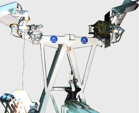
Figure 2: The experimental setup.

In this section, experimental results are presented and show the performance of the predictor that permits the capture of a tumbling satellite even if the vision system is fully occluded by providing the prediction of the pose of the satellite based on the estimate of the full states and parameters at a given time. The Neptec Laser Camera system (LCS) [10], is used to obtain the pose measurements at a rate of 2 Hz. Figure 2 illustrates the experimental setup, whereby the mockup of a satellite is moved by a manipulator according to orbital dynamics using the concept of hybrid simulator [22, 23, 24, 25, 26] while another arm, equipped with a robotic hand, is used to autonomously approach and capture this mockup. The CAD surface model of target is imported to the 3D registration algorithm for pose estimation, see Fig. 3. For the spacecraft simulator that drives the manipulator, parameters are selected as $I=\mbox{diag}\begin{bmatrix}4&8&5\end{bmatrix}~{}\mbox{kgm}^{2}$ and $\rho_{t}=\begin{bmatrix}-0.15&0&0\end{bmatrix}^{T}~{}\mbox{m}$.

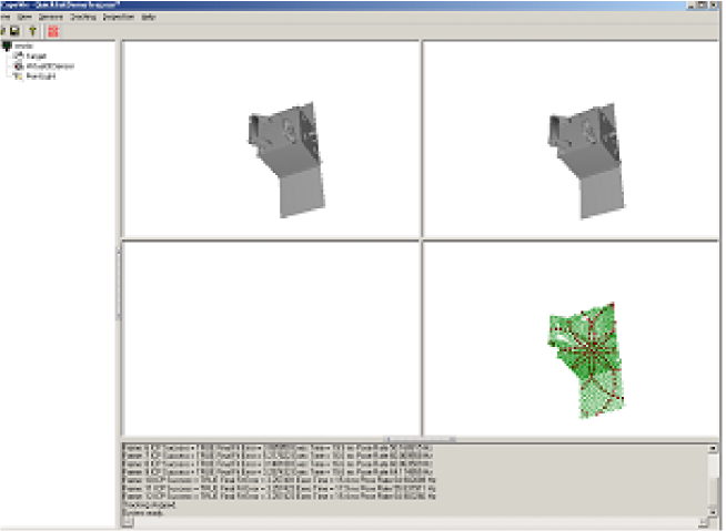
Figure 3: Surface model of target

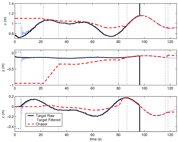
Figure 4: Cartesian position of the grasping device matching the motion of the target

The objective of this experiment is that the robotic arm autonomously capture the handle of the target satellite using the pose provided by the LCS. During the tracking of the handle, the field of view of the LCS was voluntary fully occluded and hence the EKF is to reliably provide the pose information. Figure 4 illustrates trajectories of the position measurements from the LCS (solid lines) versus the EKF outputs (dotted lines) and those of robot end-effector (dashed lines). The EKF was enabled at t=5 sec. and converges after about 9 sec. later. At t=22 sec., the chaser arm starts approaching the target satellite and it reaches a safe distance at t=34 sec. This safe distance is maintained until the autonomy engine determine that the final alignment can be performed safely. This alignment is initiated at t=80 sec. and is completed at t=87 sec. At that time, the chaser arm is tracking the target satellite. At t=96 sec., the vision system is voluntary fully occluded as we can observe by looking at the solid black line of Fig. 4. Even after the failure of the vision system to provide the pose of the satellite, the EKF continues to provide a good prediction of its pose and the tracking of the target satellite by the chasing arm continue for about 20 sec. At t=116 sec., a capture command is issued and the capture is completed successfully at t=118 sec., thus showing the excellent performance of the EKF at providing a reliable pose of the target satellite even after the failure of the vision system.

5 Conclusion

A discrete-time adaptive estimator was developed for estimating the relative pose of two free-falling satellites that move in close orbits near each other using position and orientation data provided by a laser vision system. The covariance matrix of the measurement noise was modelled in a state-dependant form. This model allows additive quaternion noise, while preserving the unit-norm property of the quaternion. The effects of orbital mechanics was incorporated in the model-based estimator for both the accurate estimation and the prediction of the relative motion. The discrete-time model, including the state-transition matrix and the covariance of the process noise were derived in closed form suitable for implementing the extended Kalman filter in real time. Experimental results illustrating the autonomous capture of a tumbling satellite with an occluded vision system were reported. The results demonstrated that the filter could accurately estimate and predict the states of the system for more than 20 seconds after the occlusion, thus permitting the successful capture of a tumbling satellite.

References

- [1] F. Aghili, “A prediction and motion-planning scheme for visually guided robotic capturing of free-floating tumbling objects with uncertain dynamics,” IEEE Transactions on Robotics, vol. 28, no. 3, pp. 634–649, June 2012.
- [2] E. Bornschlegl, G. Hirzinger, M. Maurette, R. Mugunolo, and G. Visentin, “Space robotics in Europe, a compendium,” in Proc. 7th Int. Symp. on Artificial Intelligece, Robotics, and Automation in Space: i-SAIRAS 2003, Japan, May 2003.
- [3] F. Aghili, “Active orbital debris removal using space robotics,” in International Symposium on Artificial Intelligence, Robotics and Automation in Space i-SAIRAS, Turin, Italy, Sep. 4–6 2012.
- [4] F. Aghili and K. Parsa, “Adaptive motion estimation of a tumbling satellite using laser-vision data with unknown noise characteristics,” in 2007 IEEE/RSJ International Conference on Intelligent Robots and Systems, Oct 2007, pp. 839–846.
- [5] K. Yoshida, “Engineering test satellite VII flight experiment for space robot dynamics and control: Theories on laboratory test beds ten years ago, now in orbit,” The Int. Journal of Robortics Research, vol. 22, no. 5, pp. 321–335, 2003.
- [6] F. Aghili and K. Parsa, “A reconfigurable robot with lockable cylindrical joints,” IEEE Trans. on Robotics, vol. 25, no. 4, pp. 785–797, August 2009.
- [7] D. Whelan, E. Adler, S. Wilson, and G. Roesler, “Darpa orbital express program: effecting a revolution in space-based systems,” in Small Payloads in Space, vol. 136, Nov. 2000, pp. 48–56.
- [8] F. Aghili and C. Y. Su, “Robust relative navigation by integration of icp and adaptive kalman filter using laser scanner and imu,” IEEE/ASME Transactions on Mechatronics, vol. 21, no. 4, pp. 2015–2026, Aug 2016.
- [9] F. Aghili and K. Parsa, “An adaptive vision system for guidance of a robotic manipulator to capture a tumbling satellite with unknown dynamics,” in IEEE/RSJ Int. Conf. on Intelligent Robots and Systems, Nice, France, September 2008, pp. 3064–3071.
- [10] C. Samson, C. English, A. Deslauriers, I. Christie, F. Blais, and F. Ferrie, “Neptec 3D laser camera system: From space mission STS-105 to terrestrial applications,” Canadian Aeronautics and Space Journal, vol. 50, no. 2, pp. 115–123, 2004.
- [11] U. Hillenbrand and R. Lampariello, “Motion and parameter estimation of a free-floating space object from range data for motion prediction,” in The 8th Int. Symposium on Artifcial Intelligence, Robotics and Automation in Space: i-SAIRAS 2005, Munich, Germany, Sep. 5–8 2005.
- [12] F. Aghili, M. Kuryllo, G. Okouneva, and C. English, “Fault-tolerant position/attitude estimation of free-floating space objects using a laser range sensor,” IEEE Sensors Journal, vol. 11, no. 1, pp. 176–185, Jan. 2011.
- [13] F. Aghili and K. Parsa, “Motion and parameter estimation of space objects using laser-vision data,” AIAA Journal of Guidance, Control, and Dynamics, vol. 32, no. 2, pp. 538–550, March 2009.
- [14] F. Aghili, “Optimal control for robotic capturing and passivation of a tumbling satellite with unknown dyanmcis,” in AIAA Guidance, Navigation and Control Conference, Honolulu, Hawaii, August 2008.
- [15] F. Aghili, K. Parsa, and E. Martin, “Robotic docking of a free-falling space object with occluded visual condition,” in 9th Int. Symp. on Artificial Intelligence, Robotics & Automation in Space, Los Angeles, CA, Feb. 26 – 29 2008.
- [16] F. Aghili, “Cartesian control of space manipulators for on-orbit servicing,” in AIAA Guidance, Navigation and Control Conference, Toronto, Canada, August 2010.
- [17] Y. Masutani, T. Iwatsu, and F. Miyazaki, “Motion estimation of unknown rigid body under no external forces and moments,” in IEEE Int. Conf. on Robotics & Automation, San Diego, May 1994, pp. 1066–1072.
- [18] F. Aghili, “Automated rendezvous & docking (AR&D) without impact using a reliable 3d vision system,” in AIAA Guidance, Navigation and Control Conference, Toronto, Canada, August 2010.
- [19] F. Aghili and A. Salerno, Multisensor Attitude Estimation and Applications, 1st ed. CRC Press, 2016, ch. Adaptive Data Fusion of Multiple Sensors for Vehicle Pose Estimation.
- [20] J. Breakwell and R. Roberson, “Oribtal and attitude dynamics,” Lecture notes, 1970.
- [21] F. Aghili, “A unified approach for inverse and direct dynamics of constrained multibody systems based on linear projection operator: Applications to control and simulation,” IEEE Trans. on Robotics, vol. 21, no. 5, pp. 834–849, Oct. 2005.
- [22] J.-C. Piedbœuf, F. Aghili, M. Doyon, and E. Martin, “Dynamic emulation of space robot in one-g environment using hardware-in-loop simulation,” in CISM-IFToMM Symposium on Robotics Design, Dynamics and Control, Italy, July 3–6 2002.
- [23] F. Aghili and J.-C. Piedbœuf, “Contact dynamics emulation for hardware-in-loop simulation of robots interacting with environment,” in IEEE International Conference on Robotics & Automation, Washington, USA, May 11–15 2002, pp. 534–529.
- [24] J.-C. Piedbœuf, J. de Carufel, F. Aghili, and E. Dupuis, “Task verification facility for the Canadian special purpose dextrous manipulator,” in IEEE Int. Conf. on Robotics & Automation, Detroit, Michigan, May 10–15 1999, pp. 1077–1083.
- [25] F. Aghili and M. Namvar, “Scaling inertia properties of a manipulator payload for 0-g emulation of spacecraft,” The International Journal of Robotics Research, vol. 28, no. 7, pp. 883–894, July 2009.
- [26] F. Aghili, M. Namvar, and G. Vukovich, “Satellite simulator with a hydraulic manipulator,” in IEEE Int. Conference on Robotics & Automation, Orlando, Florida, May 2006, pp. 3886–3892.