Daniel Friedan New High Energy Theory Center and Department of Physics and Astronomy,
Rutgers, The State University of New Jersey,
Piscataway, New Jersey 08854-8019 U.S.A. dfriedan@gmail.com   physics.rutgers.edu/​~friedan

Abstract
The cosmological gauge field (CGF) is a classical solution of SU(2)-weak gauge theory oscillating rapidly in time. It is the dark matter driving the CGF cosmology. A general, local, mathematically natural construction of the CGF is given here. The macroscopic properties are derived. The CGF is an irrotational perfect fluid. It provides a synchronized global time coordinate and a global rest frame. There is a conserved number density. The energy density and pressure are related by the same equation of state as derived in the CGF cosmology and used in the TOV stellar structure equations for stars made of CGF dark matter. The present construction justifies the TOV solution. Some possible routes towards testing the theory are suggested at the end.

Contents

1. 1 Introduction
   1. 1.1 The CGF cosmology and dark matter stars
   2. 1.2 Summary of the construction
   3. 1.3 Summary of the macroscopic properties
2. 2 Standard Model action
3. 3 SU(2) structure on space-time spinors
   1. 3.1 Equivalence to a four-velocity field $u^{\alpha}(x)$
   2. 3.2 A natural SU(2) spin connection
4. 4 Form of the CGF
5. 5 Equations of motion
6. 6 Solution of the equations of motion
7. 7 Energy-momentum tensor
8. 8 Irrotationality and the CGF rest frame
9. 9 Adiabatic time evolution implies a continuity equation
10. 10 Summary of the parametrization
11. 11 Low density regime
12. 12 Possibilities of detection and verification?
13. Acknowledgments

1  Introduction

1.1  The CGF cosmology and dark matter stars

If dark matter can be explained within the Standard Model then, as far as we know, the Standard Model (including some neutrino couplings) and classical General Relativity (including the cosmological constant) are the complete fundamental laws of physics which have governed the universe over all of its history since a time before the electroweak transition. A fundamental or first principles cosmology is an initial state of the SM and classical GR at the beginning of this Standard Model epoch. Such an initial state completely determines all following cosmology. The CGF cosmology [1, 2, 3, 4, 5] is a fundamental cosmology of the Standard Model epoch. It starts from a specific initial state prior to the electroweak transition. The initial state is semi-classical, a classical solution of the SM and GR corrected by small fluctuations. The initial state is completely determined by a certain Spin(4) symmetry group and a large initial energy. The Spin(4) symmetry acts as SO(4) on space, which is a 3-sphere, imposing homogeneity and isotropy. The Spin(4) acts nontrivially on the SU(2)-weak sector of the SM. The Spin(4)-symmetric SU(2)-weak gauge field has a single degree of freedom $b(t)$. This is the cosmological gauge field (the CGF). $b(t)$ is an anharmonic oscillator because the Yang-Mills hamiltonian is quartic. $b(t)$ oscillates rapidly in time because of its high initial energy. The macroscopic energy-momentum tensor of the CGF is that of perfect fluid which is non-relativistic at low density ($w\approx 0$). Its non-gravitational interactions are very small. So the CGF is dark matter. At leading order, in the classical approximation, the universe contains only the CGF dark matter. Ordinary matter is a sub-leading correction arising from fluctuations around the classical solution. There is a systematic expansion around the classical dark matter universe. This simple initial condition leads to an electro-weak transition followed by an expanding universe that contains primarily dark matter. The dark matter is a coherent effect within the Standard Model. No physics beyond the Standard Model is needed. The initial energy is the only free parameter of the classical solution, but the specific value of the initial energy does not affect the local cosmology at all, so there are effectively no free parameters. The initial energy determines the radius of curvature, so the large lower bound on the radius of curvature from observation puts a large lower bound on the initial energy. The classical solution $b(t)$ is given by an elliptic function periodic in imaginary time as well as real time, thus defining a natural temperature. The initial fluctuations of the SM fields around the classical CGF are in the thermal state determined by the Spin(4) symmetry. To check the feasibility of the CGF cosmology, it is crucial to calculate the time evolution of the initial fluctuations around the classical CGF. Overdensities in the CGF have presumably collapsed to self-gravitating bodies. The TOV stellar structure equations for stars made of the CGF dark matter fluid were solved in [4]. The solutions are shown in Figure 1. If the CGF cosmology is correct then presumably the dark matter is now in the form of such dark matter stars.

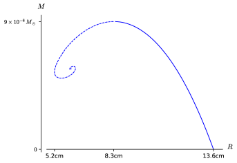
Figure 1: The curve of solutions of the TOV equations. The dashed curve are the solutions unstable against spherically symmetric pulsations. The solid curve are the (presumably) stable solutions. If the dark matter takes the form of such compact objects, microlensing observations imply that most of the dark matter must lie in objects of low mass $M<10^{-11}\,\textup{M}_{\odot}$. Such low mass CGF stars all have radius $13.6$ cm independent of the mass.

1.2  Summary of the construction

The solution of the TOV equations in [4] assumed that the non-homogeneous CGF behaves as a perfect fluid obeying the same equation of state as derived in the homogeneous, isotropic cosmology. The assumption is justified here by a general, local microscopic construction of the classical CGF in terms of the SM fields. This general construction can be used to calculate the time evolution of the density fluctuations in order to determine if and when the fluctuations end up as halos consisting of dark matter stars. The subleading corrections to the classical CGF can be calculated, in particular to find whether the interactions with the SM fields are strong enough to be used to detect the CGF. The general CGF is a solution of the SU(2)-weak gauge field equation of motion which oscillates in time on the microscopic scale

$$\ell_{0}=\frac{\hbar}{m_{\scriptscriptstyle\mathrm{Higgs}}}=5\,{\times}\,10^{-27}\text{s}\qquad\text{(in $c=1$ units)}$$ (1.1)

while varying in space at a much larger macroscopic scale $\ell$. The space-time metric is

$$\begin{gathered}ds^{2}=\ell^{2}\,g_{\mu\nu}(x)\,dx^{\mu}dx^{\nu}\qquad\text{signature }(-,+,+,+)\end{gathered}$$ (1.2)

where $g_{\mu\nu}(x)$ and $x^{\mu}$ are dimensionless quantities. Indices are raised and lowered with $g_{\mu\nu}$. Powers of the macroscopic length $\ell$ are written explicitly. $\ell$ is determined by the Einstein equation:

$$\begin{gathered}G_{\mu\nu}=8\pi G\,{\ell^{2}}g_{\mu\sigma}T^{\sigma}_{\nu}\qquad G_{\mu\nu}=O(1)\qquad T^{\sigma}_{\nu}=O\left(\frac{m_{\scriptscriptstyle\mathrm{Higgs}}}{\ell_{0}^{3}}\right)\\[4.30554pt] 1=G\ell^{2}\frac{m_{\scriptscriptstyle\mathrm{Higgs}}}{\ell_{0}^{3}}=\frac{G\ell^{2}m_{\scriptscriptstyle\mathrm{Higgs}}^{4}}{\hbar^{3}}\qquad\ell=\frac{\hbar}{m_{\scriptscriptstyle\mathrm{Higgs}}^{2}}\sqrt{\frac{\hbar}{G}}=\frac{\hbar m_{\scriptscriptstyle\mathrm{Planck}}}{m_{\scriptscriptstyle\mathrm{Higgs}}^{2}}=15.4\,\text{cm}\end{gathered}$$ (1.3)

The large ratio

$$\omega_{0}=\frac{\ell}{\ell_{0}}=\frac{m_{\scriptscriptstyle\mathrm{Planck}}}{m_{\scriptscriptstyle\mathrm{Higgs}}}=1\,{\times}\,10^{17}$$ (1.4)

suppresses spatial derivatives in the energy-momentum tensor relative to time derivatives, which is to say that the hamiltonian is ultralocal up to $O(10^{-17})$ corrections. The logic of the construction is:

1. The construction should be local in space-time, work in an arbitrary space-time metric, and be mathematically natural (generally covariant).

2. The CGF cosmology should be the special case with Spin(4) symmetry.

3. The rank-2 SU(2)-weak vector bundle can be identified with the rank-2 vector bundle of chiral spinors on space-time up to an arbitrary SU(2) gauge transformation. The gauge fields in the spinor bundle become the SU(2)-weak gauge fields. The general such identification is parametrized by a field $u^{\mu}(x)$ of time-like unit 4-vectors, $u^{\mu}u_{\mu}=-1$, $u^{0}>0$.

4. There is a mathematically natural family of SU(2) gauge fields in the spinor bundle parametrized by a single scalar function $b(x)$ on space-time.

5. The microscopic CGF solves the Yang-Mills equation in this natural family of gauge fields on the condition of rapid oscillation in time. It is a mathematically natural classical solution of the SU(2)-weak gauge theory, well-defined up to gauge equivalence.

6. The 3d wavefronts provide a global synchronized time coordinate $T(x)$ and a global rest frame.

1.3  Summary of the macroscopic properties

The macroscopic energy-momentum tensor is that of a perfect fluid of density $\rho(x)$, pressure $p(x)$, and four-velocity $u_{\alpha}(x)$,

$$T^{\alpha}_{\mu}=-u^{\alpha}u_{\mu}\rho+(\delta^{\alpha}_{\mu}+u^{\alpha}u_{\mu})p$$ (1.5)

There is a number density $n(x)$ that obeys a continuity equation,

$$\nabla_{\mu}J^{\mu}=0\qquad J^{\mu}(x)=n(x)u^{\mu}(x)$$ (1.6)

The four-velocity is irrotational,

$$u_{[\mu}\partial_{\nu}u_{\rho]}=0$$ (1.7)

Irrotationality is equivalent to existence of the global rest frame in which $u^{i}(x)=0$ and $g_{0i}(x)=0$. The CGF has two phases. At high density the SU(2) gauge symmetry is unbroken. At low density it is broken. In the broken phase the CGF is parametrized by a numerical function $k(x)$. Density, pressure, and number density are given by parametric equations

$$k\mapsto\rho(k)\qquad k\mapsto p(k)\qquad k\mapsto n(k)$$ (1.8)

which are algebraic expressions in the complete elliptical integrals $K(k)$ and $E(k)$ of the first and second kinds. $k(x)$ is the elliptic modulus that parametrizes the anharmonic oscillation of $b(x)$. The equation of state relating density and pressure is given implicitly by the parametric equations (1.8). It is the same equation of state as derived in the cosmological construction [2] and used in the TOV equations for CGF dark matter stars [4]. Details of calculations are shown in a separate note [6].

2  Standard Model action

The SM fields that participate in the CGF are the SU(2)-weak gauge field $B_{\mu}(x)$ and the SU(2) doublet Higgs field $\phi(x)$. The SU(2) covariant derivative is

$$D_{\mu}=\partial_{\mu}+B_{\mu}\qquad D_{\mu}\phi=\partial_{\mu}\phi+B_{\mu}\phi$$ (2.1)

The curvature form is

$$F_{\mu\nu}=[D_{\mu},\,D_{\nu}]=\partial_{\mu}B_{\nu}-\partial_{\nu}B_{\mu}+[B_{\mu},\,B_{\nu}]$$ (2.2)

The classical action as parametrized in [7] is

$$\frac{1}{\hbar}S_{\mathrm{gauge}} =\int\frac{1}{2g^{2}}\mathrm{tr}\left(-\ell^{-4}F_{\mu\nu}F^{\mu\nu}\right)\,\ell^{4}\sqrt{-g}\,d^{4}x\$$ (2.3)

$$\frac{1}{\hbar}S_{\mathrm{scalar}} =\int\left[\ell^{-2}D_{\mu}\phi^{\dagger}D^{\mu}\phi+\frac{1}{2}\lambda^{2}\left(\phi^{\dagger}\phi-\frac{1}{2}v^{2}\right)^{2}\right]\,\ell^{4}\sqrt{-g}\,d^{4}x$$ (2.4)

$$\begin{gathered}g=\frac{e}{\sin\theta_{W}}\qquad\cos\theta_{W}=\frac{m_{W}}{m_{Z}}\qquad\frac{gv}{2}=\frac{m_{W}}{\hbar}\qquad\lambda v=\frac{m_{\scriptscriptstyle\mathrm{Higgs}}}{\hbar}\end{gathered}$$ (2.5)

$$\begin{gathered}\alpha=\frac{e^{2}}{4\pi}=1/137.035999139(31)\qquad\frac{m_{W}}{m_{Z}}=0.88147(13)\\[4.30554pt] m_{W}=80.379(12)\,\text{\footnotesize GeV}\qquad m_{Z}=91.1876(21)\,\text{\footnotesize GeV}\qquad m_{\scriptscriptstyle\mathrm{Higgs}}=125.10(14)\,\text{\footnotesize GeV}\end{gathered}$$ (2.6)

giving tree-level parameters

$$g^{2}=0.411\qquad\lambda^{2}=0.249$$ (2.7)

The CGF probes energies on the order of $m_{\scriptscriptstyle\mathrm{Higgs}}$ but 3-momenta on the macroscopic scale $\hbar/\ell$ so there should be no appreciable renormalization of the couplings.

3  SU(2) structure on space-time spinors

3.1  Equivalence to a four-velocity field $u^{\alpha}(x)$

Let $S$ be the vector bundle of spinors over space-time. The fiber $S_{x}$ at $x$ is a four-dimensional complex vector space. Let $S^{+}$ be the rank-two sub-bundle of chiral spinors (the eigenspaces $\gamma_{5}=1$). The fiber $S^{+}_{x}$ at each point $x$ in space-time is the two-dimensional defining representation of the group Spin(1,3) = SL(2,$\mathbb{C}$). An SU(2) structure on the chiral spinors is an SU(2) subgroup of SL(2,$\mathbb{C}$) determined by a positive hermitian form on $S^{+}_{x}$. That is, $\text{SU}(2)=\text{SL}(2,\mathbb{C})\cap\text{U}(2)$. The space of SU(2) structures on $S^{+}_{x}$ is

$$\text{SL(2,$\mathbb{C}$)}/\text{SU(2)}=\text{SO(1,3)}/\text{SO(3)}=\{u^{\alpha}\colon u^{\alpha}u_{\alpha}=-1,\;u^{0}>0\}$$ (3.1)

i.e., the space of four-velocities $u^{\alpha}(x)$ at $x$. The SU(2) structures on the vector bundle $S^{+}$ are in 1-to-1 correspondence with the four-velocity fields $u^{\alpha}(x)$. Given an SU(2) structure on the chiral spinors, i.e., given a four-velocity field $u^{\alpha}(x)$, the SU(2)-weak vector bundle can be identified with $S^{+}$ up to gauge equivalence. Conversely, any such identification determines an SU(2) structure on the chiral spinors. The CGF is a natural solution of the Yang-Mills equation in the SU(2) spinor bundle arising from such an identification. The four-velocity field $u^{\alpha}(x)$ characterizing the SU(2) structure turns out to be the physical four-velocity field of the macroscopic CGF fluid. The construction is local in space-time. It extends to a global construction if no topological obstructions prevent identifying the SU(2)-weak vector bundle with the chiral spinor bundle. There are no such obstructions in the space-time $\mathbb{R}\times S^{3}$ of the CGF cosmology.

3.2  A natural SU(2) spin connection

The space-time metric is

$$ds^{2}=\ell^{2}\,g_{\mu\nu}(x)\,dx^{\mu}dx^{\nu}\qquad\text{signature }(-,+,+,+)$$ (3.2)

with $\ell=15.4\,\text{cm}$ the macroscopic length scale. The space-time orientation is expressed by the volume form $\ell^{4}\epsilon_{\mu\nu\rho\sigma}(x)$.

$$\frac{1}{4!}\epsilon_{\mu\nu\rho\sigma}\epsilon^{\mu\nu\rho\sigma}=-1$$ (3.3)

The four-velocity field $u^{\alpha}(x)$ expresses the SU(2) structure.

$$u_{\alpha}u^{\alpha}=-1\qquad u^{0}>0$$ (3.4)

The projection on the space-like tangent vectors orthogonal to $u$ is

$$P^{\alpha}_{\beta}=\delta^{\alpha}_{\beta}+u^{\alpha}u_{\beta}$$ (3.5)

The Dirac matrices $\gamma_{\mu}(x)$ act on the spinors $S_{x}$ at $x$.

$$\begin{gathered}\gamma_{\mu}\gamma_{\nu}+\gamma_{\nu}\gamma_{\mu}=2g_{\mu\nu}\qquad\gamma_{5}=\frac{i}{4!}\epsilon^{\mu\nu\rho\sigma}\gamma_{\mu}\gamma_{\nu}\gamma_{\rho}\gamma_{\sigma}\qquad\gamma_{5}^{2}=1\end{gathered}$$ (3.6)

The generators of Spin(1,3) on $S_{x}$ are

$$L_{\mu\nu}=\frac{1}{4}[\gamma_{\mu},\,\gamma_{\nu}]\qquad L_{\mu\nu}=\frac{1}{2i}\epsilon_{\mu\nu}{}^{\rho\sigma}L_{\rho\sigma}\gamma_{5}\qquad[L_{\mu\nu},\,\gamma_{5}]=0$$ (3.7)

The bundle of chiral spinors $S^{+}$ is the rank 2 subbundle of eigenspaces $\gamma_{5}(x)=1$. The subbundle $S^{-}$ is the subbundle $\gamma_{5}(x)=-1$. The positive hermitian form on $S^{+}_{x}$ associated to $u^{\alpha}(x)$ extends naturally to a positive hermitian form on $S^{-}_{x}$ and thus all of $S$ such that

$$u^{\alpha}\gamma_{\alpha}^{\dagger}=-u^{\alpha}\gamma_{\alpha}\qquad P^{\alpha}_{\beta}\gamma_{\alpha}^{\dagger}=P^{\alpha}_{\beta}\gamma_{\alpha}$$ (3.8)

The boosts relative to $u^{\alpha}(x)$ are the matrices

$$L_{\mu}=u^{\alpha}L_{\alpha\mu}\qquad u^{\mu}L_{\mu}=0\qquad L_{\mu}^{\dagger}=L_{\mu}$$ (3.9)

The matrices $iL_{\mu}$ generate SU(2) on $S^{\pm}$.

$$[L_{\mu},\,L_{\nu}]=u^{\rho}\epsilon_{\rho\mu\nu}{}^{\sigma}iL_{\sigma}\gamma_{5}\qquad L_{\mu}L_{\nu}+L_{\nu}L_{\mu}=\frac{1}{2}P_{\mu\nu}$$ (3.10)

The metric covariant derivative $\nabla_{\mu}$ acts on spinors such that

$$\nabla_{\mu}\gamma_{\nu}=0$$ (3.11)

The curvature 2-form of $\nabla_{\mu}$ is

$$F^{\text{metric}}_{\mu\nu}=[\nabla_{\mu},\,\nabla_{\nu}]=\frac{1}{2}R^{\alpha\beta}{}_{\mu\nu}L_{\alpha\beta}$$ (3.12)

$\nabla_{\mu}$ defines a Spin(1,3) connection in the spinor bundle. It does not preserve the hermitian structure, i.e. $\nabla_{\mu}\gamma_{\nu}^{\dagger}\neq\nabla_{\mu}\gamma_{\nu}$ or $\nabla_{\mu}L_{\nu}^{\dagger}\neq\nabla_{\mu}L_{\nu}$. The modified covariant derivative

$$D^{0}_{\mu}=\nabla_{\mu}-\nabla_{\mu}u^{\sigma}L_{\sigma}$$ (3.13)

defines a natural Spin(1,3) connection that does preserve the hermitian structure

$$D^{0}_{\mu}L_{\nu}=\nabla_{\mu}u^{\sigma}u_{\nu}L_{\sigma}\qquad D^{0}_{\mu}\left(L_{\nu}^{\dagger}\right)=(D^{0}_{\mu}L_{\nu})^{\dagger}$$ (3.14)

so $D^{0}_{\mu}$ defines a natural SU(2) connection in the spin bundle. Its curvature 2-form is

$$\begin{gathered}F^{0}_{\mu\nu}=[D^{0}_{\mu},\,D^{0}_{\nu}]=\left(\frac{1}{2}R^{\alpha\beta}{}_{\mu\nu}-\nabla_{\mu}u^{\alpha}\nabla_{\nu}u^{\beta}\right)[L_{\alpha},\,L_{\beta}]\end{gathered}$$ (3.15)

4  Form of the CGF

The general SU(2) covariant derivative is

$$D_{\mu}=D^{0}_{\mu}+B_{\mu}\qquad B_{\mu}=iL_{\alpha}B_{\mu}^{\alpha}(x)$$ (4.1)

The CGF has the naturally distinguished form

$$D_{\mu}=D^{0}_{\mu}+iL_{\mu}b(x)$$ (4.2)

parametrized by a scalar function $b(x)$ on space-time. $b(x)$ oscillates in time on the microscopic scale while varying smoothly in space on the macroscopic scale. That is,

$$b(x)=\omega_{0}b_{0}(\zeta)\qquad\zeta=\omega_{0}T(x)$$ (4.3)

where $b_{0}(\zeta)$ is a smooth function of $\zeta$ and also depends (implicitly for now) smoothly on $x^{\mu}$ and where $T(x)$ is a smooth time coordinate,

$$\partial_{\mu}T\partial^{\mu}T<0\qquad\partial_{0}T>0$$ (4.4)

We can take $b_{0}(\zeta)$ to be periodic in $\zeta$ with period $2\pi$ by reparametrizing $T(x)$. Alternatively, the wave form of $b(x)$ determines $T(x)$. Count wavefronts by consecutive integers $n$. Then $T(x)=2\pi n/\omega_{0}$ on the wavefronts and interpolates smoothly between them.

5  Equations of motion

Scalar field equation of motion.

Re-write the scalar action (2.4) in terms of the dimensionless scalar field $\hat{\phi}={v\phi}/{\sqrt{2}}$.

$$\frac{1}{\hbar}S_{\mathrm{scalar}}=\int\frac{1}{8\lambda^{2}}\left[\frac{4}{\omega_{0}^{2}}D_{\mu}\hat{\phi}^{\dagger}D^{\mu}\hat{\phi}+\left(\hat{\phi}^{\dagger}\hat{\phi}-1\right)^{2}\right]\,\omega_{0}^{4}\sqrt{-g}\,d^{4}x$$ (5.1)

with

$$D_{\mu}\hat{\phi}^{\dagger}D^{\mu}\hat{\phi} =(D^{0}_{\mu}+B_{\mu})\hat{\phi}^{\dagger}(D^{0\mu}+B^{\mu})\hat{\phi}$$ (5.2)

$B_{\mu}B^{\mu}$ is a multiple of the identity, $B_{\mu}B^{\mu}=\frac{1}{2}\mathrm{tr}(B_{\mu}B^{\mu})$, so

$$D_{\mu}\hat{\phi}^{\dagger}D^{\mu}\hat{\phi} =D^{0}_{\mu}\hat{\phi}^{\dagger}D^{0\mu}\hat{\phi}-\hat{\phi}^{\dagger}B_{\mu}D^{0\mu}\hat{\phi}+D^{0}_{\mu}\hat{\phi}^{\dagger}B^{\mu}\hat{\phi}-\hat{\phi}^{\dagger}\hat{\phi}\frac{1}{2}\mathrm{tr}(B_{\mu}B^{\mu})$$ (5.3)

Assume $\hat{\phi}(x)$ is smooth and $B_{\mu}=O(\omega_{0})$. Then to leading order in $\omega_{0}$

$$\frac{1}{\hbar}S_{\mathrm{scalar}}=\int\frac{1}{8\lambda^{2}}\left[2\hat{\phi}^{\dagger}\hat{\phi}\,\mathrm{tr}\left(-\frac{B_{\mu}B^{\mu}}{\omega_{0}^{2}}\right)+\left(\hat{\phi}^{\dagger}\hat{\phi}-1\right)^{2}\right]\,\omega_{0}^{4}\sqrt{-g}\,d^{4}x$$ (5.4)

The CGF has $B_{\mu}=\omega_{0}b_{0}iL_{\mu}$. To leading order in $\omega_{0}$,

$$\frac{1}{\hbar}S_{\mathrm{scalar}}=\int\frac{1}{8\lambda^{2}}\left[\,(\hat{\phi}^{\dagger}\hat{\phi})^{2}+3\left(b_{0}^{2}-\frac{2}{3}\right)\hat{\phi}^{\dagger}\hat{\phi}+1\right]\,\omega_{0}^{4}\sqrt{-g}\,d^{4}x$$ (5.5)

Since $b_{0}$ is oscillating rapidly compared to the macroscopic scale, $b_{0}^{2}$ can be replaced by its time average $\langle\,b_{0}^{2}\,\rangle$. The leading order scalar equations of motion are then

$$\hat{\phi} =0\quad\; \langle\,b_{0}^{2}\,\rangle \geq\frac{2}{3}$$       unbroken phase (5.6)

$$\hat{\phi}^{\dagger}\hat{\phi} =1-\frac{3}{2}\langle\,b_{0}^{2}\,\rangle\quad\; \langle\,b_{0}^{2}\,\rangle <\frac{2}{3}$$       broken phase

The solutions with $\langle\,b_{0}^{2}\,\rangle\geq\frac{2}{3}$, are in the unbroken phase. The solutions with $\langle\,b_{0}^{2}\,\rangle>\frac{2}{3}$, are in the broken phase. In the broken phase, when $\hat{\phi}^{\dagger}\hat{\phi}>0$, the direction of $\hat{\phi}(x)$ is determined by the next-to-leading order equations of motion.

Gauge field equation of motion

Vary the gauge action (2.3) and the leading order scalar action (5.4) wrt the gauge field to obtain the gauge field equation of motion at leading order in $\omega_{0}$.

$$\begin{gathered}0=\frac{D^{\nu}F_{\mu\nu}}{\omega_{0}^{3}}+\frac{g^{2}\hat{\phi}^{\dagger}\hat{\phi}}{4\lambda^{2}}\frac{B_{\mu}}{\omega_{0}}+O(\omega_{0}^{-1})\end{gathered}$$ (5.7)

where

$$\begin{gathered}B_{\mu}=O(\omega_{0})\qquad D^{0}_{\mu}B_{\nu}=O(\omega_{0}^{2})\qquad F_{\mu\nu}=D^{0}_{[\mu}B_{\nu]}+[B_{\mu},\,B_{\nu}]+O(\omega_{0})\end{gathered}$$ (5.8)

For the CGF,

$$\begin{gathered}B_{\mu}=ibL_{\mu}\qquad b=\omega_{0}b_{0}(\zeta)\qquad\zeta=\omega_{0}T\\[4.30554pt] \frac{1}{\omega_{0}^{2}}F_{\mu\nu}=\frac{db_{0}}{d\zeta}\partial_{[\mu}TiL_{\nu]}-b_{0}^{2}[L_{\mu},\,L_{\nu}]+O(\omega_{0}^{-1})\end{gathered}$$ (5.9)

The leading order equation of motion (5.7) is

$$0 =\left(-\partial^{\nu}T\partial_{\nu}T\frac{d^{2}b_{0}}{d\zeta^{2}}+\frac{g^{2}\hat{\phi}^{\dagger}\hat{\phi}}{4\lambda^{2}}b_{0}+2b_{0}^{3}\right)iL_{\mu}+\left(\frac{d^{2}b_{0}}{d\zeta^{2}}\partial_{\mu}T\partial^{\nu}T\right)iL_{\nu}$$ (5.10)

$$\qquad\qquad{}-\left(3b_{0}\frac{db_{0}}{d\zeta}\partial^{\nu}T\right)[L_{\mu},\,L_{\nu}]$$

Contracting with $u^{\mu}$ gives

$$0=\left(\frac{d^{2}b_{0}}{d\zeta^{2}}u^{\mu}\partial_{\mu}T\partial^{\nu}T\right)iL_{\nu}$$ (5.11)

But $d^{2}b_{0}/d\zeta^{2}\neq 0$ and $u^{\mu}\partial_{\mu}T\neq 0$ so $\partial^{\nu}TL_{\nu}=0$ so

$$u_{\mu}=-a_{\ell}\partial_{\mu}T\qquad u^{\mu}\partial_{\mu}T=\frac{1}{a_{\ell}}\qquad\partial_{\nu}T\partial^{\nu}T=-\frac{1}{a_{\ell}^{2}}$$ (5.12)

for $a_{\ell}(x)$ a dimensionless function on space-time. Using (5.12) in (5.10), the leading order gauge field equation of motion becomes the anharmonic oscillator equation

$$0=\frac{1}{a_{\ell}^{2}}\frac{d^{2}b_{0}}{d\zeta^{2}}+\left(\frac{g^{2}\hat{\phi}^{\dagger}\hat{\phi}}{4\lambda^{2}}\right)b_{0}+2b_{0}^{3}$$ (5.13)

which has conserved energy

$$H=\frac{1}{2}\frac{1}{a_{\ell}^{2}}\left(\frac{db_{0}}{d\zeta}\right)^{2}+\frac{1}{2}\left(\frac{g^{2}\hat{\phi}^{\dagger}\hat{\phi}}{4\lambda^{2}}\right)b_{0}^{2}+\frac{1}{2}b_{0}^{4}$$ (5.14)

The oscillator is parametrized by $a_{\ell}^{2}$ and $\hat{\phi}^{\dagger}\hat{\phi}$ which vary slowly in space-time compared to the period of oscillation.

6  Solution of the equations of motion

The Jacobi elliptic function $\operatorname{cn}(z,k)$ satisfies

$$1=\left(\frac{d\operatorname{cn}}{dz}\right)^{2}+(1-2k^{2})\operatorname{cn}^{2}+k^{2}\operatorname{cn}^{4}$$ (6.1)

and has period $4K$ in $z$, where $K(k)$ is the complete elliptic integral of the first kind. So

$$\begin{gathered}F(\zeta,k)=\frac{k\operatorname{cn}(z,k)}{\zeta^{\prime}}\qquad\zeta=\frac{2\pi}{4K}z\qquad\zeta^{\prime}=\frac{2\pi}{4K}\end{gathered}$$ (6.2)

has period $2\pi$ in $\zeta$ and satisfies

$$\frac{k^{2}(1-k^{2})}{2\zeta^{\prime}{}^{4}}=\frac{1}{2}\left(\frac{dF}{d\zeta}\right)^{2}+\frac{1}{2}\left(\frac{1-2k^{2}}{\zeta^{\prime}{}^{2}}\right)F^{2}+\frac{1}{2}F^{4}$$ (6.3)

The anharmonic energy equation (5.14) is solved by

$$\begin{gathered}b_{0}(\zeta)=\frac{1}{a_{\ell}}F(\zeta,k)\end{gathered}$$ (6.4)

when $F$ satisfies

$$\begin{gathered}a_{\ell}^{4}{H}=\frac{1}{2}\left(\frac{dF}{d\zeta}\right)^{2}+\frac{1}{2}\left(\frac{g^{2}\hat{\phi}^{\dagger}\hat{\phi}\,a_{\ell}^{2}}{4\lambda^{2}}\right)F^{2}+\frac{1}{2}F^{4}\end{gathered}$$ (6.5)

which is

$$\begin{gathered}H=\frac{k^{2}(1-k^{2})}{2\zeta^{\prime}{}^{4}a_{\ell}^{4}}\qquad\frac{g^{2}\hat{\phi}^{\dagger}\hat{\phi}}{4\lambda^{2}}=\frac{1-2k^{2}}{\zeta^{\prime}{}^{2}a_{\ell}^{2}}\end{gathered}$$ (6.6)

The time average of $b_{0}^{2}$ is

$$\langle\,b_{0}^{2}\,\rangle=\left(k^{2}-1+\frac{E}{K}\right)\frac{1}{\zeta^{\prime}{}^{2}a_{\ell}^{2}}$$ (6.7)

where $E(k)$ is the complete elliptic integral of the second kind. In the unbroken phase, $\hat{\phi}=0$, (6.6) implies

$$k^{2}=\frac{1}{2}\qquad H=\frac{1}{8\zeta^{\prime}{}^{4}a_{\ell}^{4}}$$ (6.8)

The solution is parametrized by $a_{\ell}$ in the range

$$\langle\,b_{0}^{2}\,\rangle=\left(\frac{E}{K}-\frac{1}{2}\right)\frac{1}{\zeta^{\prime}{}^{2}a_{\ell}^{2}}\geq\frac{2}{3}$$ (6.9)

In the broken phase,

$$\begin{gathered}\hat{\phi}^{\dagger}\hat{\phi}=1-\frac{3}{2}\langle\,b_{0}^{2}\,\rangle=1-\frac{3}{2}\left(k^{2}-1+\frac{E}{K}\right)\frac{1}{\zeta^{\prime}{}^{2}a_{\ell}^{2}}\end{gathered}$$ (6.10)

Equation (6.6) gives $H$ and $\hat{\phi}^{\dagger}\hat{\phi}$ as functions of $k$ and $a_{\ell}$. Equations (6.10) and (6.6) combine to give $a_{\ell}$ as a function of $k$.

$$\begin{gathered}\zeta^{\prime}{}^{2}a_{\ell}^{2}=\frac{4\lambda^{2}}{g^{2}}(1-2k^{2})+\frac{3}{2}\left(k^{2}-1+\frac{E}{K}\right)\qquad 0\leq k^{2}\leq\frac{1}{2}\end{gathered}$$ (6.11)

So $H$, $\hat{\phi}^{\dagger}\hat{\phi}$, and $a_{\ell}$ are functions of $k$. The solution in the broken phase is parametrized by $k$ in the range $0\leq k^{2}\leq 1/2$. This is a classical solution of the equations of motion at leading order in $\omega_{0}$. The leading order solution should deform to an exact classical solution order by order in $\omega_{0}^{-2}$. This needs to be verified. And the semi-classical expansion around the classical solution should be stable against small fluctuations. This was shown for the Spin(4)-symmetric CGF in [3].

7  Energy-momentum tensor

The CGF scalar and gauge energy-momentum tensors at leading order in $\omega_{0}$ are

$$T^{\phi}{}^{\mu}_{\nu} =\frac{\hbar}{\ell_{0}^{4}}\frac{1}{8\lambda^{2}}\left[\hat{\phi}^{\dagger}\hat{\phi}\,b_{0}^{2}\left(3e^{\mu}e_{\nu}-P^{\mu}_{\nu}\right)+\left(\hat{\phi}^{\dagger}\hat{\phi}-1\right)^{2}\left(e^{\mu}e_{\nu}-P^{\mu}_{\nu}\right)\right]$$ (7.1)

$$T^{\mathrm{gauge}}{}^{\mu}_{\nu} =\frac{\hbar}{\ell_{0}^{4}}\frac{1}{2g^{2}}\left[\frac{1}{a_{\ell}^{2}}\left(\frac{db_{0}}{d\zeta}\right)^{2}+b_{0}^{4}\right]\left(3u^{\mu}u_{\nu}+P^{\mu}_{\nu}\right)$$

So the CGF energy-momentum tensor is that of a perfect fluid

$$\begin{gathered}T^{\mu}_{\nu}=\rho u^{\mu}u_{\nu}+pP^{\mu}_{\nu}\end{gathered}$$ (7.2)

Expressed in units of the microscopic energy density

$$\rho_{0}=\frac{m_{\scriptscriptstyle\mathrm{Higgs}}}{\ell_{0}^{3}}=\frac{\hbar}{\ell_{0}^{4}}$$ (7.3)

the density $\rho$ is

$$\frac{\rho}{\rho_{0}} =\frac{3}{2g^{2}}\left[\frac{1}{a_{\ell}^{2}}\left(\frac{db_{0}}{d\zeta}\right)^{2}+b_{0}^{4}\right]+\frac{3}{8\lambda^{2}}\hat{\phi}^{\dagger}\hat{\phi}\,b_{0}^{2}+\frac{1}{8\lambda^{2}}\left(\hat{\phi}^{\dagger}\hat{\phi}-1\right)^{2}$$ (7.4)

$$=\frac{3}{g^{2}}H+\frac{1}{8\lambda^{2}}\left(\hat{\phi}^{\dagger}\hat{\phi}-1\right)^{2}$$

The pressure $p$ is

$$\frac{p}{\rho_{0}} =\frac{1}{2g^{2}}\left[\frac{1}{a_{\ell}^{2}}\left(\frac{db_{0}}{d\zeta}\right)^{2}+b_{0}^{4}\right]-\frac{1}{8\lambda^{2}}\hat{\phi}^{\dagger}\hat{\phi}\,b_{0}^{2}-\frac{1}{8\lambda^{2}}\left(\hat{\phi}^{\dagger}\hat{\phi}-1\right)^{2}$$ (7.5)

$$=\frac{1}{g^{2}}H-\frac{1}{4\lambda^{2}}\hat{\phi}^{\dagger}\hat{\phi}\,b_{0}^{2}-\frac{1}{8\lambda^{2}}\left(\hat{\phi}^{\dagger}\hat{\phi}-1\right)^{2}$$

$$=\frac{1}{g^{2}}H-\frac{1}{4\lambda^{2}}\hat{\phi}^{\dagger}\hat{\phi}\,\langle\,b_{0}^{2}\,\rangle-\frac{1}{8\lambda^{2}}\left(\hat{\phi}^{\dagger}\hat{\phi}-1\right)^{2}$$

where the rapidly oscillating term $b_{0}^{2}$ is replaced by its time average in the last step. In the unbroken phase where $\phi=0$,

$$\frac{\rho}{\rho_{0}}=\frac{3}{g^{2}}H+\frac{1}{8\lambda^{2}}\qquad\frac{p}{\rho_{0}}=\frac{1}{g^{2}}H-\frac{1}{8\lambda^{2}}$$ (7.6)

with $H$ given by equation (6.8). The fluid is parametrized by $a_{\ell}$ in the range (6.9). In the broken phase,

$$\frac{\rho}{\rho_{0}}=\frac{3}{g^{2}}H+\frac{9}{32\lambda^{2}}\langle\,b_{0}^{2}\,\rangle^{2}\qquad\frac{p}{\rho_{0}}=\frac{1}{g^{2}}H-\frac{\hat{\phi}^{\dagger}\hat{\phi}}{4\lambda^{2}}\langle\,b_{0}^{2}\,\rangle-\frac{9}{32\lambda^{2}}\langle\,b_{0}^{2}\,\rangle^{2}$$ (7.7)

$H$ and $\hat{\phi}^{\dagger}\hat{\phi}$ are given by equation (6.6) and $\langle\,b_{0}^{2}\,\rangle$ is given by equation (6.7). Equation (6.11) parametrizes all three by $k$ in the range $0\leq k^{2}\leq 1/2$. The equation of state is the same as calculated in the CGF cosmology [2]. The parametrization of $\rho$ and $p$ by $a_{\ell}$ in the unbroken phase and by $k$ in the broken phase is the same as in the CGF cosmology.

8  Irrotationality and the CGF rest frame

The CGF is irrotational (at leading order in $\omega_{0}$) because $u_{\mu}=-a_{\ell}\partial_{\mu}T$ so $\partial_{[\nu}u_{\rho]}=(u_{[\rho}\partial_{\nu]}a_{\ell})/a_{\ell}$ so

$$u_{[\mu}\partial_{\nu}u_{\rho]}=0$$ (8.1)

Conversely, if $u^{\mu}(x)$ is an arbitrary irrotational four-velocity field then there exists a time coordinate $T(x)$ such that $P_{\mu}^{\alpha}\partial_{\alpha}T=0$, i.e. $\partial_{\mu}T=-u_{\mu}(u^{\alpha}\partial_{\alpha}T)$. Space-time is the union of the space-like hypersurfaces parametrized by $T$.

$$M^{(3)}_{t}=\left\{x\colon\;T(x)=t\right\}$$ (8.2)

The hypersurfaces $M^{(3)}_{t}$ are orthogonal to $u_{\mu}$,

$$v^{\mu}u_{\mu}=0\quad\Longleftrightarrow\quad v^{\mu}\partial_{\mu}T=0$$ (8.3)

The flow lines of the vector field $u^{\mu}\partial_{\mu}$ identify the hypersurfaces $M^{(3)}_{t}$ with each other. So space-time is parametrized as $\mathbb{R}\times M^{(3)}_{0}$ with coordinates $x^{\mu}=(T,x^{i})$. The four-velocity and metric are

$$\begin{gathered}u^{\alpha}=(a_{\ell}^{-1},0,0,0)\qquad g_{00}=-a_{\ell}^{2}\qquad g_{0i}=0\\[4.30554pt] ds^{2}=\ell^{2}g_{\mu\nu}dx^{\mu}dx^{\nu}=\ell^{2}a_{\ell}(x)^{2}\left[-(dT)^{2}+g^{(3)}_{ij}(x)dx^{i}dx^{j}\right]\end{gathered}$$ (8.4)

This is the CGF rest frame.

9  Adiabatic time evolution implies a continuity equation

In the rest frame the leading order action of the CGF is

$$\begin{gathered}\frac{1}{\hbar}S_{\scriptscriptstyle\mathrm{CGF}}=\int d\zeta\,\int d^{3}x\sqrt{\det g^{(3)}_{ij}}\;\frac{3\omega_{0}^{3}}{g^{2}}\left[-\frac{1}{2}\left(\frac{dF}{d\zeta}\right)^{2}+A_{1}F^{2}+\frac{1}{2}F^{4}+A_{0}\right]\\[4.30554pt] A_{1}=\frac{g^{2}\hat{\phi}^{\dagger}\hat{\phi}a_{\ell}^{2}}{8\lambda^{2}}\qquad A_{0}=\frac{g^{2}(\hat{\phi}^{\dagger}\hat{\phi}-1)^{2}a_{\ell}^{4}}{24\lambda^{2}}\end{gathered}$$ (9.1)

Each volume element $d^{3}x$ of the CGF is an independent anharmonic oscillator. The oscillator coupling constants vary slowly in time compared to the period of oscillation. In such an adiabatic time evolution, the adiabatic invariant $\oint pdq$ stays constant in time, where $q$ is the oscillator degree of freedom, $p$ its canonical conjugate, and the integral is over one period of oscillation. The conjugate variable to $q=F$ is

$$p=d^{3}x\,\sqrt{\det g^{(3)}_{ij}}\;\hbar\frac{3\omega_{0}^{3}}{g^{2}}\frac{dF}{d\zeta}$$ (9.2)

so the adiabatic invariant (measured in quanta) is

$$\frac{1}{2\pi\hbar}\oint pdq=d^{3}x\,\sqrt{\det g^{(3)}_{ij}}\;N(x)$$ (9.3)

$$N(x) =\frac{3\omega_{0}^{3}}{2\pi g^{2}}\int_{0}^{2\pi}\left(\frac{dF}{d\zeta}\right)^{2}d\zeta=\frac{\omega_{0}^{3}}{g^{2}\zeta^{\prime}{}^{2}}\left[1-k^{2}+(2k^{2}-1)\frac{E}{K}\right]$$ (9.4)

Its constancy in time is the equation

$$0=\frac{\partial}{\partial T}\left(\sqrt{\det g^{(3)}_{ij}}\;N\right)$$ (9.5)

Written covariantly this is the continuity equation for a conserved number density $n(x)$.

$$n(x)=\frac{N(x)}{(\ell a_{\ell})^{3}}\qquad J^{\mu}(x)=n(x)\,\ell^{3}\,u^{\mu}(x)\,\sqrt{-g}\,d^{4}x\qquad\partial_{\mu}J^{\mu}(x)=0$$ (9.6)

$n(x)$ is the density of quanta.

10  Summary of the parametrization

Define functions of the elliptic parameter $k^{2}$,

$$\begin{gathered}C_{1}=\frac{1}{2}{k^{2}(1-k^{2})}\qquad C_{2}=1-2k^{2}\\[4.30554pt] C_{3}=k^{2}-1+\frac{E}{K}\qquad C_{4}=\zeta^{\prime}\left[1-k^{2}+(2k^{2}-1)\frac{E}{K}\right]\qquad\zeta^{\prime}=\frac{2\pi}{4K}\end{gathered}$$ (10.1)

The density, pressure, and number density are functions of two variables, $k$ and $\hat{a}={\zeta^{\prime}}a_{\ell}$,

$$\frac{\rho}{\rho_{0}} =\frac{1}{\hat{a}^{4}}\frac{3}{g^{2}}C_{1}+\frac{1}{8\lambda^{2}}\left(\frac{4\lambda^{2}}{g^{2}}\frac{C_{2}}{\hat{a}^{2}}-1\right)^{2}$$ (10.2)

$$\frac{p}{\rho_{0}} =\frac{1}{\hat{a}^{4}}\frac{1}{g^{2}}(C_{1}-C_{2}C_{3})-\frac{1}{8\lambda^{2}}\left(\frac{4\lambda^{2}}{g^{2}}\frac{C_{2}}{\hat{a}^{2}}-1\right)^{2}$$

$$\ell_{0}^{3}n =\frac{1}{\hat{a}^{3}}\frac{1}{g^{2}}C_{4}$$

The fluid is parametrized by a one-dimensional subset of this two-parameter space,

$$\begin{array}[]{r@{\quad}c@{\qquad}l}\text{unbroken phase}\colon&k^{2}=\frac{1}{2}&0<\hat{a}^{2}\leq\frac{3}{2}C_{3}\\[8.61108pt] \text{broken phase}\colon&0\leq k^{2}\leq\frac{1}{2}&\hat{a}^{2}=\frac{4\lambda^{2}}{g^{2}}C_{2}+\frac{3}{2}C_{3}\end{array}$$ (10.3)

The unbroken phase is parametrized by $\hat{a}(x)$, the broken phase by $k(x)$. The parametrization and therefore the equation of state is the same as in the cosmological construction.

11  Low density regime

In the limit $k(x)\rightarrow 0$,

$$K=\frac{\pi}{2}\left(1+\frac{k^{2}}{4}+\frac{9k^{4}}{64}\right)+O(k^{6})\qquad E=\frac{\pi}{2}\left(1-\frac{k^{2}}{4}-\frac{3k^{4}}{64}\right)+O(k^{6})$$ (11.1)

from which, at leading order in $k^{2}$,

$$\begin{gathered}\zeta^{\prime}=1\qquad\hat{a}^{2}=a_{\ell}^{2}=\frac{4\lambda^{2}}{g^{2}}\qquad ds^{2}=\ell^{2}\frac{4\lambda^{2}}{g^{2}}\left[-(dT)^{2}+g^{(3)}_{ij}(x)dx^{i}dx^{j}\right]\\[8.61108pt] \frac{\rho}{\rho_{0}}=\frac{3g^{2}}{32\lambda^{4}}k^{2}=0.600k^{2}\qquad\frac{p}{\rho_{0}}=\frac{9}{256}\frac{g^{4}}{\lambda^{4}}\left(\frac{1}{g^{2}}-\frac{1}{8\lambda^{2}}\right)k^{4}\qquad n=\frac{1}{\ell_{0}^{3}}\frac{3}{16}\frac{g}{\lambda^{3}}k^{2}\end{gathered}$$ (11.2)

Small $k$ is the low density regime ${\rho}/{\rho_{0}}\ll 1$. The low density equation of state is

$$\begin{gathered}p=\frac{c_{a}}{2}\frac{\rho^{2}}{\rho_{0}}\qquad c_{a}=\frac{\lambda^{2}\left(8\lambda^{2}-g^{2}\right)}{g^{2}}=0.992\end{gathered}$$ (11.3)

The density of quanta is related to the energy density by

$$\begin{gathered}n=\frac{2\lambda}{g}\frac{\rho}{m_{\scriptscriptstyle\mathrm{Higgs}}}=\frac{\rho}{m_{W}}\end{gathered}$$ (11.4)

so each quantum of the fluid has energy $m_{W}$. A fluid mass $M$ consists of $M/M_{W}$ quanta. The average dark matter density at the present time is

$$\langle\,\rho_{\scriptscriptstyle\mathrm{CDM}}\,\rangle_{\text{now}}=\Omega_{\scriptscriptstyle\mathrm{CDM}}\,\rho_{c}=2.3\,{\times}\,10^{-27}\text{kg}/\mathrm{m}^{3}=4\,{\times}\,10^{-56}\,\rho_{0}$$ (11.5)

where $\rho_{c}={3H_{0}^{2}}/{8\pi G}$ is the critical density and $\Omega_{\scriptscriptstyle\mathrm{CDM}}=0.27$. By (11.2),

$$\langle\,k^{2}\,\rangle_{\text{now}}=\frac{32\lambda^{4}}{3g^{2}}\frac{\langle\,\rho_{\scriptscriptstyle\mathrm{CDM}}\,\rangle_{\text{now}}}{\rho_{0}}=7\,{\times}\,10^{-56}$$ (11.6)

well within the low density regime. The TOV stellar structure equations were solved in [4] using the equation of state given by (10.2). Figure 1 shows the solutions as a spiral curve in the radius-mass plane. The curve is parametrized by the central density $\rho_{\text{central}}$ starting from $\rho_{\text{central}}=0$, $M=0$. A result from the 1960’s says that the solutions are unstable against radial pulsations except on the curve segment going from $M=0$ to the maximum mass [8, section 4.2.2 and references therein]. The maximum mass is $M_{\max}=9.15\,{\times}\,10^{-6}\textup{M}_{\odot}$ with central density $\rho_{\max}=0.799\rho_{0}$ corresponding to $k^{2}_{\max}=0.341$. This is in the broken phase but not in the low density regime. The TOV solutions can be stable only in the range $0<k^{2}_{\text{central}}<k^{2}_{\max}$. Presumably all of these solutions actually are stable. Microlensing observations imply that, if the halo dark matter is in the form of such compact objects, almost all the dark matter is in objects of mass less than $10^{-11}\textup{M}_{\odot}$ [9]. The star mass in the low density regime is $M=5\,{\times}\,10^{-5}\textup{M}_{\odot}\,k^{2}_{\text{central}}$ so $M=10^{-11}\textup{M}_{\odot}$ corresponds to $k^{2}_{\text{central}}=2\,{\times}\,10^{-7}$. So almost all of the CGF dark matter fluid should be in the low density regime.

12  Possibilities of detection and verification?

To find ways to detect the CGF, it will be necessary to calculate subleading effects — the interactions between the SM fields and the CGF — and to calculate the mass spectrum of CGF stars in the halos and in the local region.

1. If the dark matter halo is composed of dark matter stars, microlensing constrains their masses to be small. The small mass CGF stars all have diameter 27 cm independent of mass. 21 cm radiation will scatter off such stars. The halo might glow slightly in 21 cm radiation with a brightness depending on the interaction of the CGF with the electromagnetic field and on the mass spectrum of CGF stars.

2. The CGF oscillation frequency in proper time is $m_{W}/\hbar$. An electron-positron collider sitting near energy $m_{W}$ (or $2m_{W}$) might see a resonance effect when a CGF star passes through the interaction region, depending on the strength of the interactions and the local mass spectrum of CGF stars.

The CGF must satisfy the constraints of galaxy formation.

1. The initial fluctuations of the CGF have to be calculated, along the lines of [1, 2, 3]. The CGF fluctuations should satisfy the basic constraint on the initial spectrum of dark matter fluctuations.

2. The time evolution of the initial CGF fluctuations is to be calculated in the classical CGF dark matter universe. Ordinary matter is a subleading correction. Can subleading interactions radiate binding energy during gravitational collapse? Do the CGF fluctuations evolve in time to form galactic halos? of dark matter stars? with what mass spectrum? What is the local mass spectrum? Might the irrotationality of CGF dark matter explain the spherical shape of the dark matter halos?