Wigner’s Friend paradoxes: consistency with weak-contextual and weak-macroscopic realism models

Abstract

Wigner’s friend paradoxes highlight contradictions between measurements made by Friends inside a laboratory and superobservers outside a laboratory, who have access to an entangled state of the measurement apparatus. The contradictions lead to no-go theorems for observer-independent facts, thus challenging concepts of objectivity. Here, we examine the paradoxes from the perspective of establishing consistency with macroscopic realism. We present versions of the Brukner-Wigner-friend and Frauchiger-Renner paradoxes in which the spin-$1/2$ system measured by the Friends corresponds to two macroscopically distinct states. The local unitary operations $U_{\theta}$ that determine the measurement setting $\theta$ are carried out using nonlinear interactions, thereby ensuring measurements need only distinguish between the macroscopically distinct states. The macroscopic paradoxes are perplexing, seemingly suggesting there is no objectivity in a macroscopic limit. However, we demonstrate consistency with a contextual weak form of macroscopic realism (wMR): The premise wMR asserts that the system can be considered to have a definite spin outcome $\lambda_{\theta}$, at the time after the system has undergone the unitary rotation $U_{\theta}$ to prepare it in a suitable pointer basis. We further show that the paradoxical outcomes imply failure of deterministic macroscopic local realism, and arise when there are unitary interactions $U_{\theta}$ occurring due to a change of measurement setting at both sites, with respect to the state prepared by each Friend. In models which validate wMR, there is a breakdown of a subset of the assumptions that constitute the Bell-Locality premise. A similar interpretation involving a weak contextual form of realism exists for the original paradoxes.

I Introduction

The Wigner’s friend paradox concerns a gedanken experiment in which inconsistencies arise between observations recorded by experimentalists either inside or outside the laboratory (wigner-original, ). There is a distinction between systems that have undergone a “collapse” into an eigenstate due to measurement, and systems which remain entangled with the laboratory apparatus. The inconsistencies can be quantified in the form of Brukner’s no-go theorem for “observer-independent facts”, that a record of the results of measurements exists in a way that can be viewed consistently between observers (brukner, ). The no-go theorem applies to an extended Wigner’s friend paradox for two laboratories, and adopts the Locality assumption. The inconsistencies have been further highlighted by the Frauchiger-Renner paradox (fr-paradox, ). As experiments support quantum predictions (proietti, ; griffith, ), the paradoxes challenge the concept of objectivity. This has motivated much further work (proietti, ; sudbery, ; bub, ; healey, ; bohmian-fr, ; griffith, ; losada-wigner-friend, ; fr-proposal-exp, ; wigner-weak, ; scalable, ; Lostaglio, ; Zukowski2021, ; Baumann2021, ; Castellani2021, ; Leegwater, ; Brukner2022, ) including analyses involving consistent histories (losada-wigner-friend, ), Bohmian models (bohmian-fr, ), weak measurements (wigner-weak, ), timeless formulations (Baumann2021, ), and strong “local friendliness” no-go theorems (griffith, ).

In this paper, we present macroscopic versions of Brukner’s Wigner’s friend and Frauchiger-Renner paradoxes in which all measurements leading to the inconsistent results are performed on a system “which has just two macroscopically distinguishable states available to it” (s-cat, ; frowis, ). This includes the initial system measured by the Friends in each laboratory, which is normally considered to be microscopic. The consequence is that one can apply, for each system and measurement, the definition of macroscopic realism put forward by Leggett and Garg (legggarg-1, ; emary-review, ). Leggett and Garg’s macroscopic realism (MR) asserts that the system actually be in one or other state at any given time, meaning that the outcome of a measurement distinguishing between the two macroscopically-distinct states has a predetermined value.

With this definition, it would seem at first glance impossible to obtain consistency between macroscopic realism and the Wigner’s friend paradoxes, which suggest there is no objectivity between observers for the outcomes of quantum measurements on a macroscopic spin. The paradoxes as applied to macroscopic qubits become especially puzzling, because apparently then there is no basis for objectivity even in a macroscopic limit.

In this paper, we examine the relationship of the paradoxes with MR, giving a resolution of the apparent inconsistencies. We consider two forms of MR, a deterministic form (dMR) which we show is negated by the paradoxes, and a weaker form (wMR) which we show is consistent with the quantum predictions, and is similar to Bell’s idea of macroscopic ’beables’ (bell-found, ). The resolution is based on the dynamics of the unitary interaction $U_{\theta}$ that determines the measurement settings for spin measurements $S_{\theta}$. In a contextual model of quantum mechanics, the state after the interaction is different to that before. We demonstrate that the premise of MR as applied to the state after the dynamics $U_{\theta}(t)$ takes place is consistent with the quantum predictions: The premise of MR as applied to the state before the dynamics $U_{\theta}(t)$ takes place is falsified by the quantum predictions. This leads to the two definitions of MR (manushan-bell-cat-lg, ; ghz-cat, ; delayed-choice-cats, ). The first is a weaker (more minimal) assumption, referred to as weak macroscopic realism (wMR). The second definition is a stronger assumption that postulates predetermined variables prior to all stages of measurement, along the lines of classical mechanics, and is referred to as deterministic macroscopic realism (dMR).

We therefore propose an interpretation that validates an objective macroscopic realism, in which there is a predetermined value $\lambda_{\theta.i}$ for the outcome of the measurement on the macroscopic two-state system, in accordance with wMR. The system is objectively in a state of definite qubit value $\lambda_{\theta,i}$, at the time $t_{i}$ once the system has undergone the appropriate unitary rotation $U_{\theta}$ to prepare it in the suitable basis. The records of the Friends and the superobservers agree on such values. The paradoxical outcomes between the two types of observers (Friends and superobservers) illustrate a failure of dMR, which we show manifests as a violation of a macroscopic Brukner-Wigner-Bell inequality in both the extended Wigner’s friend experiment, and the Frauchiger-Renner version.

We further show that the inconsistencies between the different observers arise where there are two nonzero unitary rotations, $U_{\theta}$ and $U_{\phi}$, giving a change of measurement setting $\theta$ and $\phi$ of the superobservers with respect to the Friends, at both available laboratories. In this case, the assumption of Locality is justified by dMR, but not by wMR. The predictions that violate Brukner-Wigner-Bell or Bell inequalities are therefore not inconsistent with wMR.

In fact, the premise of wMR implies a partial locality, which asserts no-disturbance to the value of $\lambda_{\theta,i}$ for the state created at the time $t_{i}$, after the local unitary $U_{\theta}(t)$ has taken place. This is regardless of any unitary interaction $U_{\phi}$ occurring at the other laboratory. However, the premise wMR does not imply locality in the full sense: It cannot be assumed that the outcome of a spin measurement $S_{\theta}$ at one laboratory $A$ is independent of the measurement choice $\phi$ occurring at the other laboratory, if the local unitary $U_{\theta}$ at $A$ has not yet been performed.

The formulation of the macroscopic paradoxes is achieved by a direct mapping of the microscopic gedanken experiment onto a macroscopic one, the spin qubits $|$$\uparrow\rangle$ and $|\downarrow\rangle$ corresponding to two macroscopically distinct orthogonal states. We illustrate with two examples: two coherent states $|\alpha\rangle$ and $|-\alpha\rangle$ where $\alpha\rightarrow\infty$, and two groups of $N$ correlated spins. The unitary operations $U_{\theta}$ required for the measurement of a spin component $S_{\theta}$ are realised by a Kerr Hamiltonian $H_{NL}$, or else a sequence of CNOT gates.

The interpretation given in this paper motivates a similar interpretation for the original paradoxes, where the Friends make microscopic spin measurements. In that interpretation, wMR is replaced by a weak version of local realism (wR or wLR), which specifies a predetermined value $\lambda_{\theta,i}$ for the outcome of a measurement $S_{\theta}$, for the system prepared at time $t_{i}$ after the unitary interaction $U_{\theta}$ determining the choice of measurement setting $\theta$ has been carried out. The interaction $U_{\theta}$ prepares the system with respect to a measurement basis, in a state given as the superposition $|\uparrow\rangle_{\theta}+|\downarrow\rangle_{\theta}$ of eigenstates of the spin observable $S_{\theta}$. In this contextual model, the state is only completely described once the measurement basis is specified. Similar contextual models have been given for Bell violations (philippe-grang-context, ; manushan-bell-cat-lg, ) and, in a full probabilistic formulation, for quantum measurement (DrummondReid2020, ).

Overview of paper: The paper is organized as follows. In Section II, we summarise the Wigner’s friend and Frauchiger-Renner gedanken paradoxes. We illustrate the fully macroscopic versions of the paradoxes in Section III, where we show a violation of the Brukner-Bell-Wigner inequality. In Section IV, we demonstrate the failure of deterministic macroscopic (local) realism (dMR) for both paradoxes. Weak macroscopic realism (wMR) is explained in Section V, where it is shown how the weak form of realism can be compatible with violations of the Brukner-Bell-Wigner and CHSH-Bell inequalities. We prove a sequence of Results for wMR. In Section VI, the consistency of the paradoxes with wMR is illustrated by way of an explicit wMR model. This is done by comparing with the predictions of certain quantum mixtures that are valid from one or other of the Friends’ perspective. A conclusion is given in Section VII.

II Wigner’s friend paradoxes

II.1 Observer-independent facts no-go theorem: Bell-Wigner test

We first summarise the theorem introduced by Brukner for the Wigner’s friend paradox (brukner, ). A spin-$1/2$ system is in a closed laboratory $L$ where Wigner’s friend $F$ can make a measurement on a spin-$1/2$ system, to measure the $z$ component, $\sigma_{z}$. This means that the spin system will become entangled with a second more macroscopic system that exists in the laboratory. (Ultimately, as each piece of apparatus becomes entangled, the macroscopic apparatus becomes the Friend themselves). From the Friend’s perspective, after the measurement, the system has collapsed into a state that has a definite value for the spin $S_{z}$ measurement. To Wigner, who is outside the laboratory, the Friend’s measurement is described by a unitary interaction, where the combined state of the spin and Friend is given by

$$|\Phi\rangle_{SF} =\frac{1}{\sqrt{2}}\left(|\uparrow\rangle_{z}|F_{z+}\rangle+|\downarrow\rangle_{z}|F_{z-}\rangle\right).$$ (1)

Here, $|\uparrow\rangle_{z}$ and $|\downarrow\rangle_{z}$ are the eigenstates of $\sigma_{z}$. The $|F_{z+}\rangle$ and $|F_{z-}\rangle$ are states for the macroscopic measuring apparatus, which we might envisage to be a pointer on a measurement dial, that indicate the result of the measurement to be either a positive outcome $+1$ (spin “up”), or a negative outcome $-1$ (spin “down”) respectively. Wigner’s description of the combined state is that of a superposition. Hence, the interpretation of the overall state of the laboratory is different, or unclear, since the superposition is not equivalent to the mixture of the two states $|\uparrow\rangle_{z}|F_{z+}\rangle$ and $|\uparrow\rangle_{z}|F_{z+}\rangle$.

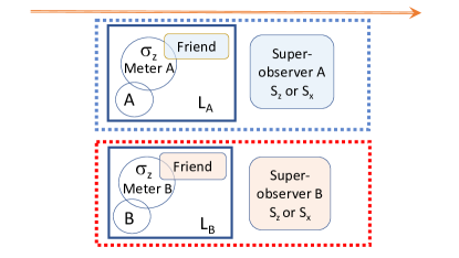
Figure 1: Wigner’s friend paradox: The two entangled systems $A$ and $B$ are prepared and then separated into laboratories $L_{A}$ and $L_{B}$. The Friends in each laboratory measure the spin $\sigma_{z}$ of the local system, using a macroscopic meter. The superobservers outside each laboratory can measure the local macroscopic spins, $S_{z}$ or $S_{x}$, of the entire Lab systems. The arrow depicts the direction of time, meaning that the superobservers make their measurements after those of the Friends.

A no-go theorem relating to the paradox was presented by Brukner, who established a theoretical framework in which one can account for observer-independent facts. The notion of observer-dependent facts is tested by carrying out a Bell-Wigner experiment. Based on the work of Brukner, a violation of a Bell-Wigner inequality implies a failure in the conjunction of: (1) Locality; (2) Free choice (freedom for all parties to choose their measurement settings; and (3) Observer-independent facts (a record from a measurement should be a fact of the world that all observers can agree on). The difference between a Bell test and a Bell-Wigner test lies in the third assumption; a Bell-Wigner test assumes observer-independent facts, while a Bell test assumes predetermined measurement outcomes. Locality is defined by Bell in the original derivation of Bell’s inequalities, and implies no instantaneous influences between spacelike-separated systems.

Brukner considered a pair of superobservers (Alice and Bob) who can carry out experiments on two separate laboratories $L_{A}$ and $L_{B}$ that consist of spin-$1/2$ systems and the superobservers’ Friends, Charlie and Debbie, respectively (Figure 1). Measurement settings $A_{1}$ and $A_{2}$ correspond to the observational statements of Charlie and Alice, while the measurement settings $B_{1}$ and $B_{2}$ correspond to the observational statements of Debbie and Bob. The conjunction of the assumptions leads to the Bell-Wigner inequality in the form of a Clauser-Horne-Shimony-Holt (CHSH) Bell inequality (cshim-review-2, ; bell-found, ; chsh, ; bell-brunner-rmp, )

$$S=|\langle A_{1}B_{1}\rangle+\langle A_{1}B_{2}\rangle+\langle A_{2}B_{1}\rangle-\langle A_{2}B_{2}\rangle|\leq 2.$$ (2)

A violation would imply a contradiction with the assumptions.

It has been shown that the inequality can be violated (brukner, ). For our work, it will prove convenient to consider two strategies, one involving measurements of $S_{z}$ and $S_{x}$ as in the original example, and the other involving measurements of $S_{z}$ and $S_{y}$. We therefore propose that Charlie and Debbie receive an entangled state of spin-$1/2$ particles given as

$$|\psi_{\pm}\rangle =-\sin\frac{\theta}{2}|\phi^{\mp}\rangle+\varepsilon_{\pm}\cos\frac{\theta}{2}|\psi^{+}\rangle$$

$$=-\sin\frac{\theta}{2}{\color[rgb]{0,0,0}(}{\color[rgb]{0,0,0}|\uparrow\rangle_{z,C}|\uparrow\rangle_{z,D}\mp|\downarrow\rangle_{z,C}|\downarrow\rangle_{z,D})/\sqrt{2}}$$

$$\ \ +\varepsilon_{\pm}\cos\frac{\theta}{2}{\color[rgb]{0,0,0}(}{\color[rgb]{0,0,0}|\uparrow\rangle_{z,C}|\downarrow\rangle_{z,D}+|\downarrow\rangle_{z,C}|\uparrow\rangle_{z,D})/\sqrt{2}}$$ (3)

where $|\phi^{\mp}\rangle=\frac{1}{\sqrt{2}}\left(|\uparrow\rangle_{z,C}|\uparrow\rangle_{z,D}\mp|\downarrow\rangle_{z,C}|\downarrow\rangle_{z,D}\right)$ and $|\psi^{+}\rangle=\frac{1}{\sqrt{2}}\left(|\uparrow\rangle_{z,C}|\downarrow\rangle_{z,D}+|\downarrow\rangle_{z,C}|\uparrow\rangle_{z,D}\right)$, with $\varepsilon_{+}=1$ and $\varepsilon_{-}=i$. The subscripts $C$ and $D$ denote the spin states prepared in Charlie and Debbie’s laboratories. We define two initial states, $|\psi_{+}\rangle$ and $|\psi_{-}\rangle$, which will allow violation of the inequality (2) for the pair of measurements $S_{z}$ and $S_{x}$, and the pair of measurements $S_{z}$ and $S_{y}$, respectively.

Next, Charlie and Debbie each perform a measurement. After completing their measurement on the system prepared in $|\psi_{\pm}\rangle$, the overall state becomes

$$|\tilde{\Psi}_{\pm}\rangle =-\sin\frac{\theta}{2}|\Phi^{-}\rangle+\varepsilon_{\pm}\cos\frac{\theta}{2}|\Psi^{+}\rangle\,,$$ (4)

where

$$|\Phi^{\mp}\rangle = \frac{1}{\sqrt{2}}\left(|A_{up}\rangle|B_{up}\rangle\mp|A_{down}\rangle|B_{down}\rangle\right)$$

$$|\Psi^{+}\rangle = \frac{1}{\sqrt{2}}\left(|A_{up}\rangle|B_{down}\rangle+|A_{down}\rangle|B_{up}\rangle\right)$$ (5)

with $|A_{up}\rangle=|\uparrow\rangle_{z,C}|C_{z+}\rangle_{C}$, $|A_{down}\rangle=|\downarrow\rangle_{z,C}|C_{z-}\rangle_{C}$, $|B_{up}\rangle=|\uparrow\rangle_{z,D}|D_{z+}\rangle_{D}$, and $|B_{down}\rangle=|\downarrow\rangle_{z,D}|D_{z-}\rangle_{D}$. Here, $|C_{z\pm}\rangle_{C}$ and $|D_{z\pm}\rangle_{D}$ are the states of the macroscopic measurement apparatus (the Friends) in the respective laboratories.

For the choice of initial state $|\psi_{+}\rangle$, we consider the measurement settings

$$A_{1}\equiv A_{z} = |A_{up}\rangle\langle A_{up}|-|A_{down}\rangle\langle A_{down}|$$

$$A_{2}\equiv A_{x} = |A_{up}\rangle\langle A_{down}|+|A_{down}\rangle\langle A_{up}|$$ (6)

corresponding to macroscopic spin $z$ and spin $x$ measurements in Charlie’s laboratory, and

$$B_{1}\equiv B_{z} = |B_{up}\rangle\langle B_{up}|-|B_{down}\rangle\langle B_{down}|$$

$$B_{2}\equiv B_{x} = |B_{up}\rangle\langle B_{down}|+|B_{down}\rangle\langle B_{up}|$$ (7)

corresponding to macroscopic spin $z$ and spin $x$ measurements in Debbie’s laboratory. The Bell-Wigner CHSH inequality for this case is

$$S=|\langle A_{z}B_{z}\rangle+\langle A_{z}B_{x}\rangle+\langle A_{x}B_{z}\rangle-\langle A_{x}B_{x}\rangle|\leq 2.$$ (8)

It has been shown that this inequality is violated for $\theta=\pi/4$ with $S=-2\sqrt{2}$.

On the other hand, for the choice of initial state $|\psi_{-}\rangle$, we consider the measurement settings

$$A_{1}\equiv A_{z} = |A_{up}\rangle\langle A_{up}|-|A_{down}\rangle\langle A_{down}|$$

$$A_{2}\equiv A_{y} = (|A_{up}\rangle\langle A_{down}|-|A_{down}\rangle\langle A_{up}|)/i$$ (9)

corresponding to macroscopic spin $z$ and spin $y$ measurements in Charlie’s laboratory, and

$$B_{1}\equiv B_{z} = |B_{up}\rangle\langle B_{up}|-|B_{down}\rangle\langle B_{down}|$$

$$B_{2}\equiv B_{y} = (|B_{up}\rangle\langle B_{down}|-|B_{down}\rangle\langle B_{up}|)/i$$ (10)

corresponding to macroscopic spin $z$ and spin $y$ measurements in Debbie’s laboratory. The Bell-Wigner CHSH inequality for this case is

$$S=\langle A_{z}B_{z}\rangle+\langle A_{z}B_{y}\rangle+\langle A_{y}B_{z}\rangle-\langle A_{y}B_{y}\rangle\leq 2$$ (11)

This the case of interest in this paper. We evaluate the correlations as follows. Directly, we find

$$\langle A_{z}B_{z}\rangle=-\cos\theta.$$

To evaluate $\langle A_{z}B_{y}\rangle$, we write the state in the new basis, by noting the standard transformation

$$|\uparrow\rangle_{y} = \frac{1}{\sqrt{2}}(|\uparrow\rangle_{z}+i|\downarrow\rangle_{z})$$

$$|\downarrow\rangle_{y} = \frac{1}{\sqrt{2}}(|\uparrow\rangle_{z}-i|\downarrow\rangle_{z})$$ (12)

where $|\uparrow\rangle_{y}$ and $|\downarrow\rangle_{y}$ are the eigenstates of the Pauli spin $\sigma_{y}$, with eigenvalues $+1$ and $-1$ respectively. Hence $|\uparrow\rangle_{z}=(|\uparrow\rangle_{y}+|\downarrow\rangle_{y})/\sqrt{2}$ and $|\downarrow\rangle_{z}=-i(|\uparrow\rangle_{y}-|\downarrow\rangle_{y})/\sqrt{2}$. Substituting, we find

$$\langle A_{z}B_{y}\rangle = \langle A_{y}B_{z}\rangle=-\sin\theta$$

$$\langle A_{y}B_{y}\rangle = \cos\theta.$$

The Bell-Wigner inequality is violated with $|S|=2\sqrt{2}$ for $\theta=\pi/4$. An experimental test supporting the predictions of quantum mechanics has been carried out by Proietti et al. (proietti, ).

II.2 Frauchiger-Renner paradox

Here we outline the Frauchiger-Renner paradox (fr-paradox, ) which also examines the Wigner friend’s thought experiment, arriving at a contradiction between the Friends inside the laboratories and the observers outside. We follow the summary given by Losada et al. (losada-wigner-friend, ).

First, a biased quantum coin tossed by the Friend $F_{A}$ in laboratory $A$ gives outcomes $h$ and $t$ with probabilities $1/3$ and $2/3$ respectively. If the outcome is $h$ or $t$, the Friend $F_{B}$ in the second laboratory $L_{B}$ creates the spin $1/2$ state $|\downarrow\rangle$ or $|\rightarrow\rangle=\frac{1}{\sqrt{2}}(|\uparrow\rangle+|\downarrow\rangle)$ respectively. Here, $|h\rangle_{z}$, $|t\rangle_{z}$ and $|\uparrow\rangle_{z}$, $|\downarrow\rangle_{z}$ are the eigenstates of the Pauli spin observables $\sigma_{z}^{A}$ and $\sigma_{z}^{B}$ for two spin $1/2$ systems at the spatially separated laboratories $L_{A}$ and $L_{B}$, respectively.

In fact, the friend $F_{A}$ has measured the state of the coin, by first coupling with a device in $L_{A}$, later measured by the Friend. The macroscopic state ultimately represents all macroscopic devices leading to the measurement outcome. The $|H\rangle_{z}$ or $|T\rangle_{z}$ are eigenstates associated with the values $h$ and $t$, for the overall laboratory $L_{A}$. The $|H\rangle_{z}$ and $|T\rangle_{z}$ are eigenstates of the observable denoted $S_{z}^{A}$. The coupling to the second laboratory $L_{B}$ is described by an interaction Hamiltonian. The system is coupled to a system in the second laboratory $B$, so that a final overall entangled state

$$|\psi_{zz}\rangle_{FR}=\frac{1}{\sqrt{3}}|H\rangle_{z}|\Downarrow\rangle_{z}+\sqrt{\frac{2}{3}}|T\rangle_{z}|\Rightarrow\rangle_{z}$$ (13)

is created. Here, $|\Rightarrow\rangle_{z}=\frac{1}{\sqrt{2}}(|\Uparrow\rangle_{z}+|\Downarrow\rangle_{z})$, where $|\Uparrow\rangle_{z}$ and $|\Downarrow\rangle_{z}$ are the overall eigenstates of the $L_{B}$ associated with the final outcomes of $\sigma_{z}^{B}$. The $|\Uparrow\rangle_{z}$ and $|\Downarrow\rangle_{z}$ are eigenstates of the observable denoted $S_{z}^{B}$.

The second step is that the external superobservers $W_{A}$ and $W_{B}$ make measurements of $S_{x}$, on the systems in $L_{A}$ and $L_{B}$ respectively. These observables are defined, so that the eigenstates of $S_{x}^{A}$ are for laboratory $L_{A}$,

$$|H\rangle_{x} = \frac{1}{\sqrt{2}}|H\rangle_{z}+\frac{1}{\sqrt{2}}|T\rangle_{z}$$ (14)

$$|T\rangle_{x} = \frac{1}{\sqrt{2}}|H\rangle_{z}-\frac{1}{\sqrt{2}}|T\rangle_{z},$$

and for $S_{x}^{B}$ of laboratory $L_{B}$,

$$|\Uparrow\rangle_{x} = \frac{1}{\sqrt{2}}|\Uparrow\rangle_{z}+\frac{1}{\sqrt{2}}|\Downarrow\rangle_{z}$$ (15)

$$|\Downarrow\rangle_{x} = \frac{1}{\sqrt{2}}|\Uparrow\rangle_{z}-\frac{1}{\sqrt{2}}|\Downarrow\rangle_{z}.$$

We first consider where $W_{A}$ and $W_{B}$ would both measure $S_{x}$. We rewrite the state (13) in terms of the different bases. We have in the new basis

$$|\psi_{xx}\rangle = \frac{\sqrt{3}}{2}|H\rangle_{x}|\Uparrow\rangle_{x}-\frac{1}{\sqrt{12}}|T\rangle_{x}|\Uparrow\rangle_{x}$$ (16)

$$\ \ \ \ -\frac{1}{\sqrt{12}}|H\rangle_{x}|\Downarrow\rangle_{x}-\frac{1}{\sqrt{12}}|T\rangle_{x}|\Downarrow\rangle_{x}.$$

From the above expression, we see that the probability is $\frac{1}{12}$ for obtaining outcomes $T$ and $\Downarrow$.

But now, if the friend $F_{B}$ had measured $\sigma_{z}$, and $W_{A}$ measures $S_{x}^{A}$ respectively, we would write

$$|\psi_{xz}\rangle=\frac{1}{\sqrt{6}}|H\rangle_{x}|\Uparrow\rangle_{z}-\frac{1}{\sqrt{6}}|T\rangle_{x}|\Uparrow\rangle_{z}+\frac{2}{\sqrt{6}}|H\rangle_{x}|\Downarrow\rangle_{z}.$$ (17)

Here, the probability to get $|T\rangle_{x}|\Downarrow\rangle_{z}$ is zero. This implies, when $W_{A}$ obtains $T$ for $S_{x}$, they can confirm with certainty that $F_{B}$ would have obtained $\uparrow$ for the measurement of $\sigma_{z}$, which in turn would seemingly imply for friend $F_{B}$ that $F_{A}$ had obtained $T$ for $\sigma_{z}$ i.e. $\lambda_{z}^{A}=-1$ (since the $\uparrow$ state for $\sigma_{z}$ at system $B$ is only created when $F_{A}$ would have obtained $T$ for $\sigma_{z}$). In the basis of $\sigma_{z}$ for $L_{A}$ and $S_{x}$ for $L_{B}$, the state is

$$|\psi_{zx}\rangle=\frac{1}{\sqrt{6}}|H\rangle_{z}\left(|\Uparrow\rangle_{x}-|\Downarrow\rangle_{x}\right)+\sqrt{\frac{2}{3}}|T\rangle_{z}|\Uparrow\rangle_{x}.$$ (18)

As the outcome $T$ for $\sigma_{z}$ is perfectly correlated with the state $|\Uparrow\rangle_{x}$, it is certain from (18) that $W_{B}$ would then get $\Uparrow$ for their measurement $S_{x}$ in lab $L_{B}.$ But (16) gives a nonzero probability for $W_{A}$ and $W_{B}$ getting $T$ and $\Downarrow$ for $S_{x}$, and this is the basis of FR paradox.

III Wigner’s friend paradoxes using cat states

In this section, we present the paradox in terms of cat states (frowis, ; s-cat, ), where the original spin $1/2$ system measured by the Friends is a macroscopic one, and the two spin $1/2$ eigenstates are macroscopically distinct states (macroscopic qubits). This is depicted in Figure 2.

An important aspect of the Wigner’s friend paradox is that the measurement of spin occurs in two stages, one of which is reversible. In the cat example, this is also true, and we will be examining a specific macroscopic realisation, so that we are able to analyse the dynamics of the measurements.

The first stage of the spin measurement is the unitary interaction $U_{\theta}$ which determines the measurement setting i.e. the component of spin that will be measured, whether $\sigma_{z}$, $\sigma_{x}$ or $\sigma_{y}$. This stage transforms an initial eigenstate into a superposition of two eigenstates: e.g. $|\uparrow\rangle\rightarrow\frac{1}{\sqrt{2}}(|\uparrow\rangle+|\downarrow\rangle)$. In a photonic Bell experiment, the unitary transformations are achieved by polarising beam splitters (PBS). The unitary rotations $U_{\theta}$ for coherent-state qubits are explained below. This stage of measurement is reversible.

The second stage of measurement occurs after the unitary rotation $U_{\theta}$. Once the unitary rotation has been performed, the measurement setting has been selected, and the system is prepared for a final stage of measurement, that we will refer to as the “pointer” measurement. This would usually include a final amplification and detection stage, involving a coupling to a meter, and a read-out to a second system e.g. an observer. We might also refer to this stage of measurement as the “collapse” stage, because, from the perspective of the observer making the measurement, this stage is irreversible.

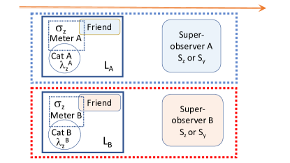
Figure 2: A macroscopic paradox with cat states: The two entangled systems $A$ and $B$ are prepared and then separated into laboratories $L_{A}$ and $L_{B}$, as in Figure 1. Here, the systems $A$ and $B$ are themselves macroscopic, meaning that the spins values $+1$ and $-1$ for $\sigma_{z}$ correspond to macroscopically distinct states. The premise of macroscopic realism asserts that the value of the spin outcome $\sigma_{z}$ is predetermined, given by a variable $\lambda_{z}$.

The paradoxes involve spin measurements on each system, $A$ and $B$. For macroscopic qubits, the spin measurements are defined according to the two-level operators. For example, the macroscopic two-state systems of the entire Labs are denoted by $|\Uparrow\rangle$ and $|\Downarrow\rangle$, and $|H\rangle$ and $|T\rangle$. The corresponding two-state spin observables are

$$S_{z}^{A} = |H\rangle\langle H|-|T\rangle\langle T|$$

$$S_{x}^{A} = |H\rangle\langle T|-|T\rangle\langle H|$$

$$S_{y}^{A} = \{|H\rangle\langle T|-|H\rangle\langle T|\}/i$$ (19)

and

$$S_{z}^{B} = |\Uparrow\rangle\langle\Uparrow|-|\Downarrow\rangle\langle\Downarrow|$$

$$S_{x}^{B} = |\Uparrow\rangle\langle\Downarrow|-|\Downarrow\rangle\langle\Uparrow|$$

$$S_{y}^{B} = \{|\Uparrow\rangle\langle\Downarrow|-|\Uparrow\rangle\langle\Downarrow|\}/i.$$ (20)

The paradoxes concern noncommuting spin measurements. We therefore will seek a unitary transformation $U_{x}^{-1}$ that transforms the eigenstates of $S_{z}$ into eigenstates of $S_{x}$:

$$|H\rangle \rightarrow (|H\rangle+|T\rangle)/\sqrt{2}$$

$$|T\rangle \rightarrow (|H\rangle-|T\rangle)/\sqrt{2}$$ (21)

or else the transformation $U_{y}^{-1}$ that transforms the eigenstates of $S_{z}$ into eigenstates of $S_{y}$:

$$|H\rangle \rightarrow (|H\rangle+i|T\rangle)/\sqrt{2}$$

$$|T\rangle \rightarrow (|H\rangle-i|T\rangle)/\sqrt{2}$$ (22)

(and similarly for $|\Uparrow\rangle$ and $|\Downarrow\rangle$).

For the initial spin $1/2$ system measured by the Friends, we propose three sorts of macroscopic qubit. The first two are presented in Appendix A. For the third, we consider the spins $|\uparrow\rangle$ and $|\downarrow\rangle$ to be macroscopic coherent states $|\alpha\rangle$ and $|-\alpha\rangle$, where $\alpha$ is large and real (Figure 2). In the limit $\alpha\rightarrow\infty$, the two states are orthogonal, and one defines two-state spin observables, for Lab $A$, as:

$$\sigma_{z}^{A} = |\alpha\rangle\langle\alpha|-|-\alpha\rangle\langle-\alpha|$$

$$\sigma_{x}^{A} = |\alpha\rangle\langle-\alpha|-|-\alpha\rangle\langle\alpha|$$

$$\sigma_{y}^{A} = \{|\alpha\rangle\langle-\alpha|-|\alpha\rangle\langle-\alpha|\}/i.$$ (23)

There is a direct mapping between the qubits $|\uparrow\rangle$ and $|\downarrow\rangle$ and the macroscopic qubits $|\alpha\rangle$ and $|-\alpha\rangle$. Similarly,

$$\sigma_{z}^{B} = |\beta\rangle\langle\beta|-|-\beta\rangle\langle-\beta|$$

$$\sigma_{x}^{B} = |\beta\rangle\langle-\beta|-|-\beta\rangle\langle\beta|$$

$$\sigma_{y}^{B} = \{|\beta\rangle\langle-\beta|-|\beta\rangle\langle-\beta|\}/i$$ (24)

where $|\beta\rangle$ and $|-\beta\rangle$ ($\beta\rightarrow\infty$) are macroscopically distinct coherent states for a mode in Lab $B$. We consider quadrature phase amplitude observables

$$\hat{X}_{A} = (\hat{a}+\hat{a}^{\dagger})/2$$

$$\hat{P}_{A} = (\hat{a}-\hat{a}^{\dagger})/2i$$ (25)

defined for a single field mode in a rotating frame, where $\hat{a}$ is the destruction operator for a system $A$ (yurke-stoler-1, ). The two states $|\alpha\rangle$ and $|-\alpha\rangle$ can be distinguished by a measurement of $\hat{X}_{A}$. The sign of the outcome gives the qubit value, whether $+1$ or $-1$. The measurement $\hat{X}_{A}$ constitutes the pointer measurement of the system. Similar observables $\hat{X}_{B}$ and $\hat{P}_{B}$ are defined for a mode $B$.

It will be necessary to also consider how to realise the first part of the measurement process, which determines whether $S_{z}$, $S_{y}$ or $S_{x}$ will be measured by the observers. The unitary transformation for $U_{y}^{A}$ can be achieved using a Kerr nonlinearity, modelled by the Hamiltonian

$$H_{NL}^{A}=\hbar\Omega\hat{n}_{A}^{2}$$ (26)

where $\hat{n}_{A}=\hat{a}^{\dagger}\hat{a}$ is the number operator. After an interaction time $t=\pi/2\Omega$, the system initially prepared in a coherent state $|\alpha\rangle$ becomes a cat state. We find (yurke-stoler-1, )

$$U_{A}(\frac{\pi}{2\Omega})|\alpha\rangle = \frac{e^{-i\pi/4}}{\sqrt{2}}(|\alpha\rangle+i|-\alpha\rangle)$$ (27)

where $U_{A}(t)=e^{-iH_{NL}^{A}t/\hbar}$. We use the notation $U_{A}\equiv U_{\pi/4}^{A}\equiv U_{A}(\frac{\pi}{2\Omega})$ to denote the transformation. Hence, for (22), we select $U_{y}=U_{A}^{-1}=(U_{\pi/4}^{A})^{-1}$. The cat states have been created for a microwave field, using a dispersive Kerr interaction $H_{NL}^{A}$ (collapse-revival-super-circuit-1, ; cat-states-super-cond, ), and similar effects are observed in Bose-Einstein condensates (collapse-revival-bec-2, ; wrigth-walls-gar-1, ). Hence, the unitary interactions associated with the measurement $S_{y}$ are performed via the inverse of $U_{\pi/4}^{A}$ and $U_{\pi/4}^{B}$. Thus, we write

$$|\pm\rangle_{y,A} =U_{\pi/4}^{A}|\pm\alpha\rangle_{z}= \frac{e^{-i\pi/4}}{\sqrt{2}}(|\pm\alpha\rangle_{z}+i|\mp\alpha\rangle_{z})$$

$$|\pm\rangle_{y,B} =U_{\pi/4}^{B}|\pm\beta\rangle_{z}= \frac{e^{-i\pi/4}}{\sqrt{2}}(|\pm\beta\rangle_{z}+i|\mp\beta\rangle_{z})$$

where we use that $U_{A}(t)=e^{-iH_{NL}^{A}t/\hbar}$ and $U_{B}(t)=e^{-iH_{NL}^{B}t/\hbar}$ as in (27). The different overall phase compared to the definition (22) does not change that the states are eigenstates of $\sigma_{y}$. This gives the required transformation, on denoting $|\pm\rangle_{z,A}\equiv|\pm\alpha\rangle_{z}$ and $|\pm\rangle_{y,A}\equiv|\pm\alpha\rangle_{y,A}$. It is straightforward to verify that $|\pm\rangle_{y,A}$ are the eigenstates of $\sigma_{y}^{A}$, given by Eq. (23) where $\alpha\rightarrow\infty$.

To rewrite the basis states for $z$ in the basis for $y$, we operate on the states by $U_{A}^{-1}$ ($U_{B}^{-1}$):

$$|\pm\alpha\rangle_{z} = U_{A}^{-1}|\pm\alpha\rangle_{y}$$ (29)

$$= \frac{e^{i\pi/4}}{\sqrt{2}}(|\pm\alpha\rangle_{y}-i|\mp\alpha\rangle_{y}).$$

More generally, for a state $|\psi\rangle$ written as a superposition of the eigenstates of $\sigma_{z}$, the transformation into the eigenstates of $\sigma_{y}$ is given by

$$U_{y}|\psi\rangle\equiv U_{A}^{-1}|\psi\rangle.$$ (30)

A similar local transformation takes place on system $B$.

The odd and even cat states $\sim|\alpha\rangle\pm|-\alpha\rangle$ which would correspond to the transformation for $U_{x}$ have also been created in the laboratory (odd-cats, ), but proposed mechanisms for generation involve conditional measurements and dissipative optical, superconducting or opto-mechanical systems (transient-cat-states-leo, ; cat-even-odd-transient, ; cats-hach, ; cat-states-wc, ; Teh2018Creation, ; Teh2020Dynamics, ). In this paper, we focus on the cat states generated by the simple unitary transformation $U_{y}^{A}$ that is realisable using $H_{NL}^{A}$. This means we focus on the versions of paradoxes that use $S_{y}$ rather than $S_{x}$ measurements. The coherent-state qubits and unitary interactions $U_{y}$ also allow macroscopic Bell violations (manushan-bell-cat-lg, ; macro-bell-lg, ), tests of macrorealism (manushan-cat-lg, ), macroscopic GHZ paradoxes (ghz-cat, ), and tests of two-dimensional macroscopic retrocausal models in delayed-choice Wheeler-Chaves-Lemos-Pienaar experiments (delayed-choice-cats, ).

III.1 Bell-Wigner tests with cat states

We now propose that the Bell-Wigner test given in Section II.A be implemented with the spins $|\uparrow\rangle_{z,C}$ and $|\downarrow\rangle_{z,C}$ realised as the macroscopic coherent states $|\alpha\rangle_{z,c}$ and $|-\alpha\rangle_{z,C}$, and the spins $|\uparrow\rangle_{z,D}$ and $|\downarrow\rangle_{z,D}$ realised as the macroscopic states $|\alpha\rangle_{z,D}$ and $|-\alpha\rangle_{z,D}$, for large $\alpha$. We explicitly write the state $|\psi_{-}\rangle$ given by Eq. (3) as

$$|\psi_{zz}\rangle_{WF} =A_{zz}{\color[rgb]{0,0,0}(}{\color[rgb]{0,0,0}|\alpha\rangle_{z,C}|\alpha\rangle_{z,D}+|-\alpha\rangle_{z,C}|-\alpha\rangle_{z,D})}$$

$$\ \ +{\color[rgb]{0,0,0}B_{zz}(|\alpha\rangle_{z,C}|-\alpha\rangle_{z,D}+|-\alpha\rangle_{z,C}|\alpha\rangle_{z,D})}$$ (31)

where $A_{zz}=-\frac{1}{\sqrt{2}}\sin\frac{\theta}{2}$ and $B_{zz}=\frac{i}{\sqrt{2}}\cos\frac{\theta}{2}$. This state describes the system prepared in the $z$ basis at both sites (Labs). A method for mapping the state (3) onto the coherent-state version (31) experimentally is presented in Refs. (cat-det-map, ; cat-bell-wang-1, ).

Charlie and Debbie then each perform a measurement. This involves coupling each system with a meter via interactions $H_{Am}$ and $H_{Bm}$, and then further couplings to the Friends in each laboratory (Lab). The overall interaction of systems with the macroscopic apparatus are described by $H_{AmF}$ and $H_{BmF}$. After completing their measurements, the overall state of the Labs becomes $|\tilde{\Psi}_{-}\rangle=-\sin\frac{\theta}{2}|\Phi^{+}\rangle+i\cos\frac{\theta}{2}|\Psi^{+}\rangle\,,$where $|\Phi^{+}\rangle$ and $|\Psi^{+}\rangle$ are given by Eq. (5), with $|A_{up}\rangle=|\alpha\rangle_{z,C}|C_{z+}\rangle_{C}$, $|A_{down}\rangle=|-\alpha\rangle_{z,C}|C_{z-}\rangle_{C}$, $|B_{up}\rangle=|\alpha\rangle_{z,D}|D_{z+}\rangle_{D}$, and $|B_{down}\rangle=|-\alpha\rangle_{z,D}|D_{z-}\rangle_{D}$. Here, $|C_{z\pm}\rangle_{C}$ and $|D_{z\pm}\rangle_{D}$ are the states of the macroscopic measurement apparatus (the friends) in the respective Labs. An example of the measurement interaction $H_{Am}$ is given in the Appendix.

At each Lab, the superobservers have the choice to measure either $S_{z}$ or $S_{y}$. To measure $S_{y}$, they first disentangle the system from the respective meters (by reversing $H_{AmF}$ or $H_{BmF}$), and then perform the unitary transformations $U_{A}^{-1}$ and $U_{B}^{-1}$ as in (29). A pointer measurement is then needed to give the final readout for $S_{y}$, meaning that the evolved system is coupled once more to the measurement apparatus, in the superobserver’s Lab.

To measure $S_{z}$, no further unitary rotation $U$ is needed, because the system given by (31) is already prepared in the basis for spin $Z$. A pointer measurement suffices to determine the final outcome for $S_{z}$. However, for simplicity of treatment, it is convenient to consider that the superobservers will in any case reverse both the couplings $H_{AmF}$ and $H_{BmF}$, regardless of their choice of measurement. This decouples the spin system from the Lab measurement apparatus (the meter and Friends), and allows a simple description of the spin systems as they evolve under any unitary rotations. In this case, a pointer measurement at a later time couples the evolved system to the meters, and measurement apparatus in the superobserver’s Lab. The final result for $S_{z}$ will agree with that of the Friend.

Consider measurements of $S_{y}^{A}$ and $S_{z}^{B}$. After reversing $H_{AmF}$ and $H_{BmF}$ and performing the necessary unitary rotations, the system is given by

$$|\psi_{zy}\rangle_{WF} =A_{zy}\{|\alpha\rangle_{z,C}|\alpha\rangle_{y,D}+i|-\alpha\rangle_{z,C}|-\alpha\rangle_{y,D}\}$$

$$\ \ +B_{zy}(-|\alpha\rangle_{z,C}|-\alpha\rangle_{y,D}+i|-\alpha\rangle_{z,C}|\alpha\rangle_{y,D})$$ (32)

where $A_{zy}=\frac{1}{2}(-\sin\frac{\theta}{2}+\cos\frac{\theta}{2})$ and $B_{zy}=\frac{1}{2}(\sin\frac{\theta}{2}+\cos\frac{\theta}{2})$. Similarly, the state of the system prepared for measurements $S_{z}^{A}$ and $S_{y}^{B}$ is

$$|\psi_{yz}\rangle_{WF} =A_{yz}\{|\alpha\rangle_{y,C}|\alpha\rangle_{z,D}+i|-\alpha\rangle_{y,C}|-\alpha\rangle_{z,D}\}$$

$$\ \ +B_{yz}(i|\alpha\rangle_{y,C}|-\alpha\rangle_{z,D}-|-\alpha\rangle_{y,C}|\alpha\rangle_{z,D})$$ (33)

where $A_{yz}=\frac{1}{2}(-\sin\frac{\theta}{2}+\cos\frac{\theta}{2})$ and $B_{yz}=\frac{1}{2}(\sin\frac{\theta}{2}+\cos\frac{\theta}{2})$. Similarly, for the measurements $S_{y}^{A}$ and $S_{y}^{B}$,

$$|\psi_{yy}\rangle_{WF} =A_{yy}{\color[rgb]{0,0,0}(}{\color[rgb]{0,0,0}|\alpha\rangle_{y,C}|\alpha\rangle_{y,D}-|-\alpha\rangle_{y}|-\alpha\rangle_{y,C})}$$

$$\ \ +B_{yy}{\color[rgb]{0,0,0}(}{\color[rgb]{0,0,0}|\alpha\rangle_{y,C}|-\alpha\rangle_{y,D})+|-\alpha\rangle_{y,C}|\alpha\rangle_{y,D})}$$ (34)

where $B_{yy}=-\frac{1}{\sqrt{2}}\sin\frac{\theta}{2}$ and $A_{yy}=\frac{1}{\sqrt{2}}\cos\frac{\theta}{2}$. Comparing with Section II.A, this gives a violation of the Bell-Wigner inequality.

III.2 Frauchiger-Renner Paradox using cat states

We now consider a test of the FR paradox based on cat states. The version of the FR paradox given in Section II.C considers the option that the observers measure either $S_{z}$ or $S_{x}$. We suppose instead that the observers at $A$ and $B$ measure either $S_{z}$ or $S_{y}$, so that we may use the transformation (27). To do this, we consider that the state initially prepared between the laboratories is

$$|\psi_{zz}\rangle = \frac{1}{\sqrt{3}}|H\rangle_{z,A}|\Downarrow\rangle_{z,B}+\frac{1}{\sqrt{3}}|T\rangle_{A}(|\Uparrow\rangle_{z,B}+i|\Downarrow\rangle_{z,B}).$$

We suppose the state is prepared with respect to the basis $S_{z}$ at each location, $A$ and $B$. A paradox can be constructed the same way as explained in Section II.B above, where the measurements of $S_{x}$ are substituted as measurements of $S_{y}$.

We now present a version of the paradox using coherent states. We suppose the initial state created between the two laboratories is

$$|\psi_{zz}\rangle_{FR} = \frac{1}{\sqrt{3}}|\alpha\rangle_{z}|-\beta\rangle_{z}$$ (36)

$$\ \ \ +\frac{1}{\sqrt{3}}|-\alpha\rangle_{z}(|\beta\rangle_{z}+i|-\beta\rangle_{z}).$$

We drop the subscripts $A$ and $B$, where it is clear that the first (second) ket refers to the first (second) system. We now suppose at each Lab that observers may make a measurement of either $\sigma_{z}$ (as performed by the Friends), or $S_{y}$ (as performed by the superobservers). The Friends’ measurement of $\sigma_{z}$ is modelled by a Hamiltonian $H_{Am}$ and $H_{Bm}$ which leads to the coupling with the meter modes. Hence,

$$|\psi_{zz,m}\rangle=e^{-iH_{Am}t/\hbar}e^{-iH_{Bm}t/\hbar}|\psi_{zz}\rangle.$$ (37)

We give an example of $H_{Am}$ in the Appendix. The state of the Labs after the Friends’ measurements is given by

$$|\psi_{zz,mF}\rangle=e^{-iH_{AmF}t/\hbar}e^{-iH_{BmF}t/\hbar}|\psi_{zz,m}\rangle$$ (38)

which describes that the Friends have themselves become coupled (entangled) with the meters. The coupling is given by interactions $H_{AmF}$ and $H_{BmF}$.

We suppose the both Wigner superobservers measure $S_{y}$. The interactions $H_{Am}$, $H_{Bm}$, $H_{AmF}$ and $H_{BmF}$ are reversed. The superobservers perform the respective local unitary interactions $U_{A}^{-1}$ and $U_{B}^{-1}$ to change the measurement settings from $z$ to $y$. After the unitary evolution corresponding to the measurement interaction, the state of the system is

$$|\psi_{yy}\rangle_{FR} = U_{A}^{-1}U_{B}^{-1}|\psi_{zz}\rangle_{FR}$$ (39)

$$= \frac{i}{2\sqrt{3}}\{-3i|\alpha\rangle_{y}|\beta\rangle_{y}-i|-\alpha\rangle_{y}|-\beta\rangle_{y}$$

$$\ \ \ +|\alpha\rangle_{y}|-\beta\rangle_{y}-|-\alpha\rangle_{y}|\beta\rangle_{y}\}.$$

Each system is then coupled to meter $M$ (in the superobservers’ Labs), using interactions $H_{AM}$ and $H_{BM}$. A pointer measurement is then made so that the superobservers may record the outcomes. We see that there is a nonzero probability of $1/12$ that both observers get outcomes $-1$ and $-1$ for measurements of $S_{y}$.

The alternative set-up is where the Friend of Lab $B$ measures $\sigma_{z}$ and superobserver $A$ measures $S_{y}$. After the reversals, the unitary interaction $U_{y}$, the state is

$$|\psi_{yz}\rangle_{FR} = U_{A}^{-1}|\psi_{zz}\rangle_{FR}$$ (40)

$$= \frac{e^{i\pi/4}}{\sqrt{6}}\{2|\alpha\rangle_{y}|-\beta\rangle_{z}+|-\alpha\rangle_{y}|\beta\rangle_{z}$$

$$\ \ \ \ -i|\alpha\rangle_{y}|\beta\rangle_{z}\}.$$

The probability of getting $-1$ for lab $B$ and $-1$ for Lab $A$ on measurements of $\sigma_{z}$ and $S_{y}$ respectively is zero: $P_{--|yz}=0$

The FR logic is as before: If from (40), Wigner superobserver $A$ gives $-1$ for $S_{y}$, it is inferred from the state $|\psi_{yz}\rangle_{FR}$ that the Friend $B$ is $+1$ for $\sigma_{z}$. But if the Friend $B$ gets the result $+1$ for $\sigma_{z}$, then one infers from the original state $|\psi_{zz}\rangle_{FR}$ at time $t_{1}$ (Eq. (LABEL:eq:fr1)) that the Friend for system $A$ measured down for $\sigma_{z}$.

Yet, considering state $|\psi_{zy}\rangle$ of (LABEL:eq:fr1) for measurements of $\sigma_{z}$ at $A$ and $S_{y}$ at $B$, if $A$ was in the state $-1$ as measured by the Friend $A$, then there is no possibility to get outcome $-1$ for $S_{y}$ at $B$. The probability of obtaining $-1$ and $-1$ for measurements $\sigma_{z}$ and $S_{y}$ is zero. This is seen by considering the measurement of $\sigma_{z}$ at $A$ and $S_{y}$ at $B$: The final state after the reversals and unitary rotation at $B$ is

$$|\psi_{zy}\rangle_{FR} = U_{B}^{-1}|\psi_{zz}\rangle_{FR}$$ (41)

$$= \frac{e^{i\pi/4}}{\sqrt{3}}\{\frac{1}{\sqrt{2}}|\alpha\rangle_{z}(|-\beta\rangle_{y}-i|\beta\rangle_{y})$$

$$\ \ \ +\sqrt{2}|-\alpha\rangle_{z}|\beta\rangle_{y}\}.$$

$P_{--|zy}=0$. This implies the impossibility to get both outcomes of $S_{y}$ being $-1$ at $A$ and $B$, in contradiction to the earlier quantum result: $P_{--|yy}=0$. This gives the paradox for a situation where all the measurements, including those initially made by the Friends, are distinguishing between two macroscopically distinct states.

IV Analysis using macroscopic realism

The macroscopic version of the paradox identifies two macroscopically distinct states available to the systems at each time $t_{i}$. This gives an inconsistency in the realistic perception of the same event by the two observers, even where those events are based on measurements of macroscopic qubits, which is puzzling. Here, we examine the definitions of macroscopic realism carefully, showing that a deterministic form of macroscopic realism is indeed falsified.

IV.1 Deterministic macroscopic (local) realism falsified

Result 4.A: The violation of the Wigner-Bell inequality for the cat-state version of the experiment implies failure of deterministic macroscopic realism.

Proof: The Wigner-Bell inequality (2) would hold, if simultaneous predetermined values for both measurements $\sigma_{y}$ and $\sigma_{z}$ are identifiable for both systems $A$ and $B$, for the state $|\psi_{zz}\rangle_{WF}$ (Eq. (3) or (31)). With this assumption, one would specify hidden variables $\lambda_{z}^{A}$ and $\lambda_{y}^{A}$ that predetermine the result of the measurement of $\sigma_{z}^{A}$ and $\sigma_{y}^{A}$ respectively, and hidden variables $\lambda_{z}^{B}$ and $\lambda_{y}^{B}$ that predetermine the result of the measurement of $\sigma_{z}^{B}$ and $\sigma_{y}^{B}$ respectively, should those measurements be performed by the Friends (or superobservers). In the set-up, the possible results for each $\lambda$ identify macroscopically distinct states for the system, as evident by writing the state $|\psi\rangle_{WF}$ in the respective bases, as in Eqs. (31)-(34).

Following the definitions of macroscopic realism given in Refs. (legggarg-1, ; manushan-bell-cat-lg, ; macro-bell-lg, ), we then refer to the assumption of the simultaneous predetermined variables as deterministic macroscopic realism (dMR). The assumption naturally includes that of Locality, but we may also specify the assumption as deterministic macroscopic (local) realism to make this clear. Following the original proofs of the Bell inequalities (chsh, ; cshim-review-2, ), the Bell-Wigner inequality follows based on the assertion of the simultaneous variables $\lambda_{z}^{A}$, $\lambda_{y}^{A}$, $\lambda_{z}^{B}$ and $\lambda_{y}^{B}$. The premise dMR also specifies that the measurements $S_{z}$ and $S_{y}$ of the superobservers are determined by the hidden variables $\lambda_{z}$ and $\lambda_{y}$, at the respective site. The assumption of dMR is therefore falsified by the violation of the Bell-Wigner inequality.

IV.2 Failure of deterministic macroscopic realism: the FR paradox

Result 4.B: The premise of dMR is also falsifiable for the FR paradox, where the assertion applies to the state $|\psi_{zz}\rangle_{FR}$ (Eq. (36)).

Proof: A Table of all possible values $\lambda_{x}$ and $\lambda_{y}$ for each system is constructed and the impossibility of the outcomes predicted by quantum mechanics is evident. The Table is given in the Appendix. In the Table, the dMR states giving a zero probability for the result $-$, $-$ for the measurements $\sigma_{z}^{A}S_{y}^{B}$ ($ZY$) and also a zero probability for getting $-$, $-$ for measurements $S_{y}^{A}\sigma_{z}^{B}$ ($Y$$Z$) can be identified. There is no possibility of an FR inconsistency, since those states for which the result is also $-$, $-$ for measurements $S_{Y}^{A}S_{y}^{B}$ ($Y$$Y$) is highlighted by the stars, but this gives a nonzero probability of $+$, $+$ for $\sigma_{z}^{A}\sigma_{z}^{B}$ ($Z$, $Z$), which is inconsistent with the initial state $|\psi_{FR}\rangle\equiv|\psi_{zz}\rangle$. The initial state has a zero probability for $+,$$+$: Therefore this prediction is not possible for the state (LABEL:eq:fr1). The Table gives a falsification of dMR, if the predictions of quantum mechanics are correct.

It is also possible to falsify dMR for the FR system, using the Bell-Wigner inequality. The choice of measurement is of either $S_{y}$ or $\sigma_{z}$ at each site. Hence we write the Bell-Wigner inequality for the two Labs, $L_{A}=A$ and $L_{B}=B$ as in (2), in terms of the average correlations of the probability distributions, where $A,B\in\{-1,+1\}$,

$$S= \left|\langle A_{z}B_{z}\rangle+\langle A_{y}B_{z}\rangle+\langle A_{z}B_{y}\rangle-\langle A_{y}B_{y}\rangle\right|\leq 2.$$ (42)

The assumption of dMR implies local hidden variables that predefine the values for $A_{1},A_{2},B_{1}$ and $B_{2}$ to be $+1$ or $-1$, implying the existence of the joint probability $p(A_{1},A_{2},B_{1},B_{2})$ whose marginals satisfy the Clauser–Horne–Shimony–Holt Bell inequality (CHSH). For the FR paradox, there are $4$ possible preparation states, $|\psi_{zz}\rangle_{FR}$, $|\psi_{yz}\rangle_{FR}$, $|\psi_{zy}\rangle_{FR}$ and $|\psi_{yy}\rangle_{FR}$. Identifying $A_{x}=\sigma_{z}^{A}$, $A_{y}=S_{y}^{A}$, $B_{z}=\sigma_{z}^{B}$, $B_{y}=S_{y}^{B}$, we evaluate from these states the following moments:

$$\langle\sigma_{z}^{A}\sigma_{z}^{B}\rangle = -1/3$$

$$\langle S_{y}^{A}\sigma_{z}^{B}\rangle = -2/3$$

$$\langle\sigma_{z}^{A}S_{y}^{B}\rangle = -2/3$$

$$\langle S_{y}^{A}S_{y}^{B}\rangle = 2/3$$ (43)

which gives a value of $S=7/3$. The violation of the inequality falsifies dMR. $\square$

V weak macroscopic realism

In this section, we show how consistency between macroscopic realism and the quantum predictions of the Wigner friends gedanken experiment can be obtained. Since deterministic macroscopic realism is falsified by the experiment, it is necessary to define macroscopic realism in a less strict sense, as given by a weaker (more minimal) assumption. This motivates the premise of weak macroscopic realism (wMR). We explain how wMR can be consistent with the Wigner friend paradoxes.

V.1 Definition of weak macroscopic realism

Weak macroscopic realism (wMR) is defined by the following two Assertions (Figure 3) (manushan-bell-cat-lg, ; ghz-cat, ):

Assertion wMR (1) There is realism for the system prepared in the “pointer superposition state” i.e. for a system prepared in the appropriate basis, for the pointer measurement: The system is regarded as having a definite predetermined value $\lambda_{\theta}$ (being $+1$ or $-1$) for the outcome $S_{\theta}$ after the unitary dynamics $U_{\theta}$ that occurs at a site, that determines the choice of measurement setting $\theta$. This value $\lambda_{\theta}$ can be considered the value of the ’record’ of the result of the measurement, even if the final pointer stage of the measurement is not actually carried out. We refer to $\lambda_{\theta}$ as the “pointer value”.

Assertion wMR (2) There is locality with respect to this pointer value: It is assumed that the value $\lambda_{\theta}$ predetermining the pointer measurement for $S_{\theta}$ is not changed by spacelike separated events e.g. a unitary rotation $U_{\phi}$ at a separated Lab. $\square$

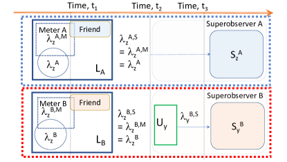
Figure 3: The weak macroscopic realism (wMR) model. The cat systems at time $t_{1}$ are described by variables $\lambda_{z}^{A}$ and $\lambda_{z}^{B}$ that predetermine outcomes for measurements of $\sigma_{z}$. After interaction with the cat systems, the meters are attributed values $\lambda_{z}^{A,M}$ and $\lambda_{z}^{B,M}$ that predetermine the outcome of the measurement on them by the Friends ($\lambda_{z}^{A,M}=\lambda_{z}^{A}$, $\lambda_{z}^{B,M}=\lambda_{z}^{B}$). These variables predetermine the outcomes ($\lambda_{z}^{A,S}$ and $\lambda_{z}^{B,S}$) if a measurement is made of $S_{z}$ by the superobservers $A$ or $B$, at the time $t_{2}$. There is no change of measurement setting at $A$. Hence $\lambda_{z}^{A,S}$ predetermines the outcome for $S_{z}^{A}$ by superobserver $A$ at time $t_{3}$, regardless of any unitary $U_{y}$ at $B$. If superobserver $B$ performs a unitary interaction $U_{y}$ to prepare the system for a (pointer) measurement $S_{y}$, then the system at time $t_{3}$ is attributed a variable $\lambda_{y}^{B,S}$ that predetermines the outcome. It is now not necessarily true that the value $\lambda_{z}^{B}$ predetermines the outcome of a future measurement $S_{z}^{B}$ (this may depend on whether there is a further unitary rotation at $A$).

For measurements of the qubit value associated with the two coherent states of system $A$, the final pointer stage of the measurement corresponds to the determination of the sign of the quadrature phase amplitude $X_{A}$. The premise wMR specifies a hidden variable $\lambda_{\theta}^{A}$ for the outcome of this pointer measurement, once the dynamics $U_{\theta}^{A}$ associated with the choice of measurement setting has occurred. This means that the predetermination is with respect to one or other spin, $S_{z}$ or $S_{y}$, not (necessarily) both simultaneously. For example, in Figure 3, the assertion applies to predetermine the outcome of $S_{z}$ at the time $t_{2}$, and then to predetermine the outcome of $S_{y}$ at the different time $t_{3}$ (after the dynamics $U_{y}$).

As part of the definition of wMR, it is assumed that the value $\lambda_{\theta}^{A}$ predetermining the pointer measurement for $S_{\theta}^{A}$ at the later time $t_{3}$ is not changed by the unitary rotation $U_{\phi}^{B}$ at $B$ (Figure 3). However, if there is a further unitary rotation $U_{\theta^{\prime}}^{A}$ at $A$, then a different variable $\lambda_{\theta^{\prime}}^{A}$ applies to the system at the later time after the interaction $U_{\theta^{\prime}}^{A}$, to predetermine the result of the new pointer measurement $S_{\theta^{\prime}}^{A}$. The wMR postulate does not assert that this value is not affected by the unitary rotation $U_{\phi}^{B}$, because here there are two unitary rotations from the initial time of preparation ($t_{2}$). The postulate wMR applies only to predetermine pointer measurements at the time after the local unitary measurement setting operation, $U$.

V.2 Achieving consistency: records and the breakdown of the Locality assumption

The assumptions of Brukner’s Bell-Wigner inequality are: (1) Locality, (2) Free choice, and (3) Observer-independent facts (a record from a measurement should be a fact of the world that all observers can agree on). The violation of the inequality implies at least one of the assumptions breaks down.Here, we address which of these assumptions can break down in a wMR-model and which records observers will agree on.

V.2.1 Records in a wMR model

We deduce which records the observers agree on in a wMR model from the definition of wMR. We find:

Result 5.B.1 (1): The Friends and superobservers agree on the record for $\sigma_{z}$: From the definition of wMR, there is predetermination of the value that would be the record of a measurement, at a time $t$, after the unitary interaction $U_{\theta}$ that determines the measurement setting $\theta$ for each Lab. Hence, in the wMR model, a definite value $\lambda_{z}^{A}$ ($\lambda_{z}^{B}$) predetermines the outcome of the Friend’s spin measurement, $\sigma_{z}$, at the Lab $A$ ($B$) (Figure 3). The superobservers can make a corresponding measurement of $S_{z}$, through various mechanisms which involve coupling to meters in the superobservers’ Labs, but do not involve a unitary interaction $U$ that gives a change of a measurement basis. The pointer measurement made by the superobservers can be regarded as a pointer measurement on the system of the Friends. In the wMR model, there is a predetermined value $\lambda_{z}^{A,S}$ ($\lambda_{z}^{B,S})$ for the outcome of the superobservers’ measurement $S_{z}^{A}$ ($S_{z}^{B}$), at the time $t_{4}$, and hence the wMR model establishes that

$$\lambda_{z}^{A,S}=\lambda_{z}^{A},\ \lambda_{z}^{B,S}=\lambda_{z}^{B}.$$

The value that gives the record of the Friends also gives the outcome that would be obtained for the measurement made by the superobservers, if they choose to measure the same spin, $S_{z}$, as the Friends (Figure 3). There is agreement for these records.

Result 5.B.1 (2): There is consistency of records between the Friends and superobservers, if only one superobserver measures a different spin component from that measured by the Friends. In the wMR model, the inconsistency arises where the two superobservers both measure a different spin (e.g. $S_{y}$). This is due to the unitary interactions $U$ that change the measurement settings. We prove this in Section V.B.2 below.

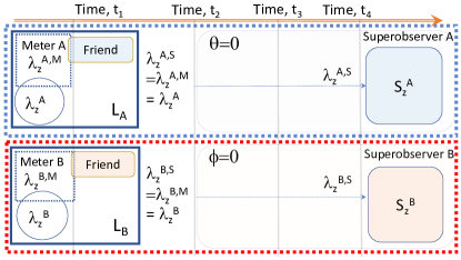
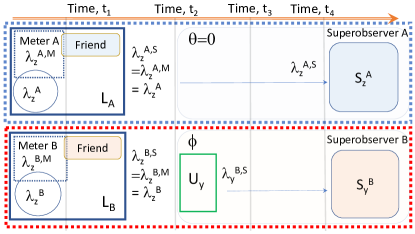
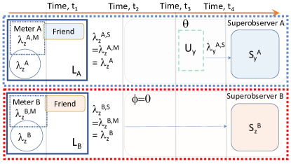
Figure 4: Resolving the paradox for consistency with weak macroscopic realism (wMR): Partial Locality. According to wMR, measuring $\langle S_{z}^{A}S_{z}^{B}\rangle$, $\langle S_{z}^{A}S_{y}^{B}\rangle$ and $\langle S_{y}^{A}S_{z}^{B}\rangle$, which involve a unitary rotation at no more than one site, gives consistent records between Friends and superobservers. The systems at time $t_{1}$ are prepared with respect to the basis for $\sigma_{z}$. The premise wMR assigns variables $\lambda_{z}^{A}$, $\lambda_{z}^{B}$, $\lambda_{z}^{A,M}$ and $\lambda_{z}^{B,M}$ to the Lab systems so that $\langle S_{z}^{A}S_{z}^{B}\rangle=\langle\lambda_{z}^{A}\lambda_{z}^{B}\rangle$ (top). The superobserver $B$ may carry out a unitary interaction $U_{y}$ to prepare the system with respect to the basis $Y$ (centre). At time $t_{3}$, the system has a definite predetermined value for $S_{y}^{B}$, given by $\lambda_{y}^{B,S}$, but the predetermination of $S_{z}^{A}$ at site $A$ is unaffected. Hence $\langle S_{z}^{A}S_{y}^{B}\rangle=\langle\lambda_{z}^{A}\lambda_{y}^{B,S}\rangle$. Similarly, $\langle S_{y}^{A}S_{z}^{B}\rangle=\langle\lambda_{y}^{A,S}\lambda_{z}^{B}\rangle$ (lower).

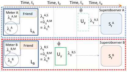
Figure 5: Resolving the paradox for consistency with weak macroscopic realism (wMR): Locality need not hold and the paradox arises where there are two rotations after the preparation, one at each site. The system is prepared at time $t_{2}$ for pointer measurements of $S_{z}$ at each site. The premise of wMR assigns variables $\lambda$ to predetermine the outcome after the unitary rotations that determine the measurement settings, $\theta$ and $\phi$. This means that when there are two unitary interactions $U_{y}$ as in the measurement of $\langle S_{y}^{A}S_{y}^{B}\rangle$ depicted in the diagram, the premise of wMR does not specify that the value of $\lambda_{y}^{A,S}$ (defined after $\lambda_{y}^{B,S}$) is independent of $\phi$, and the records are not necessarily consistent according to the inequality (8).

V.2.2 Results about Locality in a wMR model

The assumption of wMR implies only a partial locality. There is locality with respect to the pointer values $\lambda_{z}$ defined after the unitary interaction $U_{\theta}$. However, wMR does not imply Locality in the full sense. It cannot be assumed that the future outcome of $S_{y}$ at one Lab (as to be measured after the unitary interaction $U_{y}$ needed for the measurement setting) is independent of the measurement choice $\phi$ occurring at the other Lab. Hence, the observed violations of the Bell-Wigner inequality are not inconsistent with wMR. We prove the following:

Result 5.B.2: Weak macroscopic realism (wMR) does not imply the Bell-CHSH inequality.

Proof: This inequality is derived for the Wigner friend set-up by noting the variables $\lambda_{z}^{A}$, $\lambda_{y}^{A}$, $\lambda_{z}^{B}$ and $\lambda_{y}^{B}$ have the values either $+1$ or $-1$, which bounds the quantity

$$S=\lambda_{z}^{A}\lambda_{z}^{B}+\lambda_{y}^{A}\lambda_{z}^{B}+\lambda_{z}^{A}\lambda_{y}^{B}-\lambda_{y}^{A}\lambda_{y}^{B}$$ (44)

so that $|S|\leq 2$. The derivation is that these values exist in any single run, so that the bound corresponds to that for the averages. In the top diagram of Figure 4, we see we can assign the values $\lambda_{z}^{A}(t_{2})\equiv\lambda_{z}^{A}$ and $\lambda_{z}^{B}(t_{2})\equiv\lambda_{z}^{B}$ at time $t_{2}$, so that we can put

$$\langle S_{z}^{A}S_{z}^{B}\rangle=\langle\lambda_{z}^{A}(t_{2})\lambda_{z}^{B}(t_{2})\rangle=\langle\lambda_{z}^{A}\lambda_{z}^{B}\rangle.$$ (45)

We then consider the centre diagram, and define $\lambda_{y}^{B}(t_{3})\equiv\lambda_{y}^{B}(t_{3}|\theta=0)$ as the value predetermining $S_{y}^{B}$, where there is no rotation $U_{A}$ at $A$. According to wMR, the pointer measurement value at $A$ is not affected by $U_{B}$, so that

$$\langle S_{z}^{A}S_{y}^{B}\rangle=\langle\lambda_{z}^{A}\lambda_{y}^{B}(t_{3})\rangle=\langle\lambda_{z}^{A}\lambda_{y}^{B,S}\rangle.$$ (46)

Similarly, we consider the lower diagram, and define $\lambda_{y}^{A}(t_{4})\equiv\lambda_{y}^{A}(t_{4}|\phi=0)$, so that

$$\langle S_{y}^{A}S_{z}^{B}\rangle=\langle\lambda_{y}^{A}(t_{4})\lambda_{z}^{B}\rangle=\langle\lambda_{y}^{A,S}\lambda_{z}^{B}\rangle.$$ (47)

The Figure 5 shows one way to measure the moment $\langle S_{y}^{A}S_{y}^{B}\rangle$. The value of $\lambda_{y}^{B}(t_{3})$ determines $S_{y}^{B}$ independently of the future choice of $\theta$, according to wMR, because the value of the pointer measurement is specified at the time$t_{3}$ after the rotation $U_{y}$. We define $\lambda_{y}^{A}(t_{4}|\phi\neq 0)$ and $\lambda_{y}^{B}(t_{3})$, and we can say

$$\langle S_{y}^{A}S_{y}^{B}\rangle=\langle\lambda_{y}^{A}(t_{4}|\phi)\lambda_{y}^{B}(t_{3})\rangle=\langle\lambda_{y}^{A,S}\lambda_{y}^{B,S}\rangle.$$ (48)

However, from the postulate of wMR, we cannot assume the value $\lambda_{y}^{A}(t_{4})=\lambda_{y}^{A}(t_{4}|\phi)$ is independent of $\phi$. This leads us to conclude consistency of values (records) for the measurements carried out where there is no more than one unitary rotation (as in Figure 4), but not necessarily where there are two changes of measurement setting, as in the measurement of $\langle S_{y}^{A}S_{y}^{B}\rangle$ (Figure 5). $\square$

VI Consistency of the quantum predictions with the two wMR assertions

In this section, we explicitly show that the quantum predictions are consistent with the two assertions of the wMR premise, as stated by the definition in Section V.B. The first assertion is that the system prepared (after the unitary dynamics that determines the measurement setting) for the pointer measurement has a predetermined outcome $\lambda$. The second assertion is that this value is not altered by the dynamics at a different site. We show the consistency by comparing the quantum predictions with those of certain mixed states that give a particular wMR model, thereby satisfying the wMR assertions.

We will illustrate with Figures for the FR paradox. Here, the system is prepared at time $t_{1}$ in the state $|\psi_{zz}\rangle_{FR}$ given by (36). It will be useful to depict the measurement dynamics associated with the unitary rotations $U_{\theta}$ in terms of the $Q$ function. The single-mode $Q$ function $Q(\alpha_{0})=\frac{1}{4\pi}|\langle\alpha_{0}|\psi\rangle|^{2}$ defines the quantum state $|\psi\rangle$ uniquely as a positive probability distribution (husimi, ). The $Q$ function of the state $|\psi_{zz}\rangle_{FR}$ is $Q_{zz}(X_{A},P_{A},X_{B},P_{B})$, where

$${\normalcolor{\color[rgb]{0,0,1}{\normalcolor Q}_{{\normalcolor zz}}}} {\color[rgb]{0,0,1}{\normalcolor=}} {\normalcolor{\color[rgb]{0,0,1}{\normalcolor\frac{1}{\pi^{2}}|\langle\beta_{0},\alpha_{0}|\psi_{zz}\rangle|^{2}}}}$$

$${\color[rgb]{0,0,1}{\normalcolor=}} \frac{e^{-|\alpha|^{2}-|\alpha_{0}|^{2}-|\beta|^{2}-|\beta_{0}|^{2}}}{3\pi^{2}}\Bigl{\{}{\normalcolor e^{-2\alpha X_{A}-2\beta X_{B}}}$$

$$+2\cosh(2\alpha X_{A}-2\beta X_{B})+2\cos(2\alpha P_{A}-2\beta P_{B})$$

$$-2e^{-2\beta X_{B}}\sin(2\alpha P_{A})-2e^{-2\alpha X_{A}}\sin(2\beta P_{B})\Bigl{\}}.$$

Here, $\alpha_{0}=X_{A}+iP_{A}$, $\beta_{0}=X_{B}+iP_{B}$ and we consider $\alpha$, $\beta$ to be real. The first two terms in brackets give three distinct Gaussian peaks, corresponding to the three outcomes for the joint spins, originating from $|\alpha\rangle|-\beta\rangle$, $|-\alpha\rangle|\beta\rangle$ and $|-\alpha\rangle|-\beta\rangle$ in (36). These terms constitute the $Q$ function of the mixture $\rho_{zz}$ of the three states. The function $Q_{zz}$ has three sinusoidal terms, which distinguish the superposition $|\psi_{zz}\rangle_{FR}$ from the mixture $\rho_{zz}$.

The $Q$ function corresponds to the anti-normally ordered operator moments. We may compare with the probability distribution $P(\mathbf{X}_{A},\mathbf{X}_{B})$ for detecting outcomes $\mathbf{X}_{A}$ and $\mathbf{X}_{B}$ of measurements of $\hat{X}_{A}$ and $\hat{X}_{B}$. While the peaks of the marginal function $Q_{zz}(X_{A},X_{B})$ (defined by integrating over $P_{A}$ and$P_{B}$) will show extra noise, this noise is at the vacuum level. Here, we consider superpositions of macroscopically distinct coherent states, as in $|\psi_{zz}\rangle_{FR}$ (Eq. (36)), and the relevant spin measurements $\sigma_{\theta}$ or $S_{\theta}$ bin the amplitudes according to sign. To determine the spin outcomes, it is only necessary to distinguish between the macroscopically distinct components. Hence, the relative probabilities for the spin outcomes are immediately evident from the solutions (and plots) of the marginal $Q$ functions.

VI.1 Measuring $S_{z}^{A}$ and $S_{z}^{B}$: consistency with wMR

We first show consistency of the predictions for $\langle\sigma_{z}^{A}\sigma_{z}^{B}\rangle$ and $\langle S_{z}^{A}S_{z}^{B}\rangle$ with a wMR model, thereby verifying the first part of the definition of wMR. Consider the system prepared at time $t_{1}$ in the state $|\psi_{zz}\rangle$. The preparation is with respect to the $\sigma_{z}$ ($S_{z}$) “pointer basis” at each Lab, so that a pointer measurement is all that is needed to complete the measurement of $\sigma_{z}$ ($S_{z}$).

Result 6.A: The system $|\psi_{zz}\rangle$ as prepared for the spin $z$ pointer measurements gives predictions consistent with a wMR model.

Proof: The essential feature of the proof is the comparison between the predictions of the superposition as written in the pointer basis with that of the corresponding mixed state. With reference to $|\psi_{zz}\rangle=c_{11}|\alpha\rangle|\beta\rangle+c_{12}|\alpha\rangle|-\beta\rangle+c_{21}|-\alpha\rangle|\beta\rangle+c_{22}|-\alpha\rangle|-\beta\rangle$, the corresponding mixed state is

$$\rho_{zz}=\sum_{ij}|c_{ij}|^{2}\rho_{ij}$$ (50)

where $\rho_{11}=|\alpha\rangle|\beta\rangle\langle\alpha|\langle\beta|$, $\rho_{12}=|\alpha\rangle|-\beta\rangle\langle\alpha|\langle-\beta|$, $\rho_{21}=|-\alpha\rangle|\beta\rangle\langle-\alpha|\langle\beta|$ and $\rho_{22}=|-\alpha\rangle|-\beta\rangle\langle-\alpha|\langle-\beta|$. The predictions of $|\psi_{zz}\rangle$ and $\rho_{zz}$ for the joint probabilities of the pointer measurements $\sigma_{z}^{A}$ and $\sigma_{z}^{B}$ are identical. The premise of wMR asserts that hidden variables $\lambda_{z}^{A}$ and $\lambda_{z}^{B}$ are valid to predetermine the outcome of the pointer measurements $\sigma_{z}^{A}$ and $\sigma_{z}^{B}$, respectively. This interpretation holds for the mixed state $\rho_{zz}$, which describes a system that is indeed in one or other of the states comprising the mixture, and hence describable by such variables $\lambda_{z}^{A}$ and $\lambda_{z}^{B}$ at the time $t_{1}$. Hence, since the predictions for the pointer measurement on $|\psi_{zz}\rangle_{FR}$ are identical, a wMR model exists to describe the (pointer) predictions for $|\psi_{zz}\rangle_{FR}$. $\square$

It is useful to visualize this result for the macroscopic system by examining the $Q$ function, where one includes the meters. Consider $|\psi_{zz}\rangle_{FR}$ given by (36). The $Q$ function for the state (37) where the meters are explicitly included is similar to (LABEL:eq:qzz), but with four modes. The state is expanded as

$$|\psi_{zz,m}\rangle_{FR} = \frac{1}{\sqrt{3}}|\alpha\rangle_{z}|\gamma\rangle_{Am}|-\beta\rangle_{z}|-\gamma\rangle_{Bm}$$ (51)

$$\ \ \ +\frac{1}{\sqrt{3}}|-\alpha\rangle_{z}|-\gamma\rangle_{Am}(|\beta\rangle_{z}|\gamma\rangle_{Bm}$$

$$\ \ \ +i|-\beta\rangle_{z}|-\gamma\rangle_{Bm})$$

where $|\gamma\rangle$, $|-\gamma\rangle$ are coherent states for the meter of the Friend’s systems. We take $\gamma$ as large and real. The $Q$ function is $Q_{zz,m}=\frac{1}{\pi^{4}}|\langle\beta_{0},\alpha_{0},\gamma_{A},\gamma_{B}|\psi_{zz,m}\rangle_{FR}|^{2}$. Defining the complex variables $\gamma_{A}=X_{\gamma A}+iP_{\gamma A}$ for meter mode $Am$ of system $A$, and $\gamma_{B}=X_{\gamma B}+iP_{\gamma_{B}}$ for meter mode $Bm$ for system $B$, we find ($\alpha_{0}=X_{A}+iP_{A}$, $\beta_{0}=X_{B}+iP_{B}$)

$$Q_{zz,m} =\frac{e^{-|\alpha|^{2}-|\beta|^{2}-2|\gamma|^{2}}}{3\pi^{4}}e^{-|\alpha_{0}|^{2}-|\beta_{0}|^{2}-|\gamma_{A}|^{2}-|\gamma_{B}|^{2}}$$

$$\,\,\,\,\Bigl{\{}e^{-2\alpha X_{A}-2\gamma X_{\gamma A}}e^{-2\beta X_{B}-2\gamma X_{\gamma B}}$$

$$\,+2\cosh(2\alpha X_{A}+2\gamma X_{\gamma A}-2\beta X_{B}-2\gamma X_{\gamma B})$$

$$\,+2\cos(2\alpha P_{A}+2\gamma P_{\gamma A}-2\beta P_{B}-2\gamma P_{\gamma B})$$

$$\,-2e^{-2\beta X_{B}-2\gamma X_{\gamma B}}\sin(2\alpha P_{A}+2\gamma P_{\gamma A})$$

$$-2e^{-2\alpha X_{A}-2\gamma X_{\gamma A}}\sin(2\beta P_{B}+2\gamma P_{\gamma B})\Bigl{\}}.$$ (52)

The last three terms decay as $e^{-\gamma^{2}}$, and so for large $\gamma$, the solution is

$$Q_{zz,m} =\frac{e^{-P_{A}^{2}-P_{B}^{2}-P_{\gamma A}^{2}-P_{\gamma B}^{2}}}{3\pi^{4}}$$

$$\,\,\,\,\Bigl{\{}e^{-(X_{A}+\alpha)^{2}}e^{-(X_{B}+\beta)^{2}}e^{-(X_{\gamma A}+\gamma)^{2}}e^{-(X_{\gamma B}+\gamma)^{2}}$$

$$+e^{-(X_{A}-\alpha)^{2}}e^{-(X_{B}+\beta)^{2}}e^{-(X_{\gamma A}-\gamma)^{2}}e^{-(X_{\gamma B}+\gamma)^{2}}$$

$$+e^{-(X_{A}+\alpha)^{2}}e^{-(X_{B}-\beta)^{2}}e^{-(X_{\gamma A}+\gamma)^{2}}e^{-(X_{\gamma B}-\gamma)^{2}}\Bigl{\}}.$$

The final meter (pointer) measurement corresponds to the measurement of the meter quadrature amplitudes $X_{\gamma A}$ and $X_{\gamma B}$. The marginal $Q(X_{\gamma A},X_{\gamma B})$ of that describes the distribution for the measured meter outputs (as measured by the Friends) is found by integrating over all system variables as well as $P_{\gamma A}$ and $P_{\gamma B}$: We find

$$Q_{zz,m}(X_{\gamma A},X_{\gamma B}) =\frac{1}{3\pi}\Bigl{\{}e^{-(X_{\gamma A}+\gamma)^{2}-(X_{\gamma B}+\gamma)^{2}}$$

$$+e^{-(X_{\gamma A}-\gamma)^{2}}e^{-(X_{\gamma B}+\gamma)^{2}}$$

$$+e^{-(X_{\gamma A}+\gamma)^{2}}e^{-(X_{\gamma B}-\gamma)^{2}}\Bigl{\}}.$$ (54)

The three Gaussians are well-separated peaks, which represent the three distinct sets of outcomes, as expected from the components of $|\psi_{zz}\rangle_{FR}$ (Eq. (36)).

The function $Q_{zz,m}(X_{\gamma A},X_{\gamma B})$ gives the probabilities for detection of each component, for the measurement on the meter made by the Friends. We see this corresponds to $Q_{zz}(X_{A},X_{B})$ of the mixed state $\rho_{zz}$ (Eq. (50))

$$\rho_{zz}=\frac{1}{3}(\rho_{1}+\rho_{2}+\rho_{3})$$ (55)

where $\rho_{1}=|\alpha\rangle|-\beta\rangle\langle\alpha|\langle-\beta|$, $\rho_{2}=|-\alpha\rangle|\beta\rangle\langle-\alpha|\langle\beta|$ and $\rho_{3}=|-\alpha\rangle|-\beta\rangle\langle-\alpha|\langle-\beta|$, once we put $X_{\gamma A}=X_{A}$ and $X_{\gamma B}=X_{B}$, in (54). This is expected, since the meter outcomes are a measurement of the system amplitudes, $\hat{X}_{A}$ and $\hat{X}_{B}$.

We may further compare the distribution (54), which describes the final outputs of the meter-measurements made by the Friends, with that of the marginal $Q$ function

$$Q_{zz}(X_{A},X_{B}) =\frac{e^{-|\alpha|^{2}-X_{A}^{2}-|\beta|^{2}-X_{B}^{2}}}{3\pi}\Bigl{\{}{\normalcolor e^{-2\alpha X_{A}-2\beta X_{B}}}$$

$$\left.+2\cosh(2\alpha X_{A}-2\beta X_{B}){\color[rgb]{0,0,0}+2e^{-\alpha^{2}-\beta^{2}}}\right\}$$ (56)

obtained directly from the superposition $|\psi_{zz}\rangle_{FR}$ (Eq. (36)). This is derived from $Q_{zz}$ (Eq. (LABEL:eq:qzz)), by integrating over $P_{A}$ and $P_{B}$. This function corresponds to that of the systems $A$ and $B$ prior to coupling to the meter, and gives an alternative way to model the measurement by the Friends. We see that for large $\alpha=\beta$, the last term vanishes, which gives the result for $Q_{zz}(X_{A},X_{B})$ identical to (54), on replacing $X_{\gamma A}$ and $X_{\gamma B}$ with $X_{A}$ and $X_{B}$. This implies that in fact for the cat state where $\alpha$ and $\beta$ are large, the distribution for the outcomes of the pointer measurement on the superposition is indistinguishable from that for the outcomes of the pointer measurement made on the mixed state. This is evident from Figure 6. The function $Q_{zz}(X_{A},X_{B})$ of (56) is plotted in Figure 6 (far left top snapshot) and is indistinguishable from (54) of the mixture $\rho_{zz}$ (far left lower snapshot, where $X_{\gamma A}$ and $X_{\gamma B}$ are labelled $X_{A}$ and $X_{B}$).

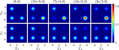
Figure 6: Contrasting the dynamics for the superposition state $|\psi_{zz}\rangle_{FR}$ and the mixed state $\rho_{zz}$. The states are initially indistinguishable but become macroscopically distinguishable under evolution. (top sequence, from left to right) We show contour plots of the marginal function $Q(X_{A},X_{B})$ at the times $(t_{a},t_{b})$, after the system has undergone a local evolution under $H_{NL}$ (Eq. (26)) for a time $t_{a}$ and $t_{b}$ in each Lab. The system begins in $|\psi_{zz}\rangle_{FR}$ (Eq. (36)) (top, far left) and evolves to $|\psi_{yz}\rangle_{FR}$ (Eq. (40) (top, far right). (lower sequence, from left to right) The system begins in $\rho_{zz}$ (Eq. (50)) and is evolved as for the top plots. Here, $\alpha=3$, $\Omega=1$.

In summary, the $Q$ function solutions for the cat and meter states give a convincing illustration of Result 6.A, that there is consistency with wMR for $\langle\sigma_{z}^{A}\sigma_{z}^{B}\rangle$, the measurements made by the Friends. The marginal $Q$ functions $Q_{zz}(X_{\gamma A},X_{\gamma B})$ and $Q_{zz}(X_{A},X_{B})$ for $|\psi_{FR}\rangle=|\psi\rangle_{zz}$ at time $t_{1}$ are indistinguishable from those of $\rho_{zz}$. Hence, the predictions for the pointer measurements of $\sigma_{z}^{A}$ and $\sigma_{z}^{B}$ on the system prepared in $|\psi_{FR}\rangle=|\psi\rangle_{zz}$ at time $t_{1}$ are consistent with a wMR model. We see however from Figure 6 that with the appropriate evolution, despite that the distinction between the $Q$ function for $|\psi_{FR}\rangle=|\psi\rangle_{zz}$ and $\rho_{zz}$ decays with $e^{-\alpha^{2}}$, the evolved states show a consistent macroscopic difference, even as $\alpha\rightarrow\infty$.

So far, the analysis concerns the measurements $\langle\sigma_{z}^{A}\sigma_{z}^{B}\rangle$ made by the Friends. We now consider $\langle S_{z}^{A}S_{z}^{B}\rangle$ as measured by the superobservers. If the system-meter state given by $|\psi_{zz,m}\rangle$ (Eq. (38)) is coupled to the Friends, then the final state being written as

$$|\psi_{zz,mF}\rangle = \frac{1}{\sqrt{3}}|\alpha\rangle_{z}|\gamma\rangle_{AmF}|-\beta\rangle_{z}|-\gamma\rangle_{BmF}$$ (57)

$$\ \ \ +\frac{1}{\sqrt{3}}|-\alpha\rangle_{z}|-\gamma\rangle_{AmF}(|\beta\rangle_{z}|\gamma\rangle_{BmF}$$

$$\ \ \ +i|-\beta\rangle_{z}|-\gamma\rangle_{BmF})$$

where $|\pm\gamma\rangle_{AmF}=|\gamma\rangle_{Am}|F\rangle_{A}$ and $|\pm\gamma\rangle_{BmF}=|\gamma\rangle_{Bm}|F\rangle_{B}$ represent the combined states of the meter and Friend in each Lab. The measurements $S_{z}$ made by the superobservers correspond to measurements on the system in a state of type (51), except that the meter systems are further coupled to second larger meters (e.g. the Friends). Since only a pointer measurement is necessary to complete the measurement of $S_{z}$, the final distribution $Q_{zz}(X_{\gamma FA},X_{\gamma FB})$ for the outcomes of the superobservers, found after integration over the unmeasured variables, is identical to (54), the distribution for the mixed state $\rho_{zz}$ (once we put $X_{\gamma FA}=X_{A}$ and $X_{\gamma FB}=X_{B}$). Hence by the same argument as above, the distribution and predictions for the final outcomes $S_{z}^{A}$ and $S_{z}^{B}$ measured by the superobservers are consistent with variables $\lambda_{z}^{A,S}$ and $\lambda_{z}^{B,S}$, giving consistency with wMR.

Moreover, we prove consistency with Result 5.B.1 (1) of wMR, that the variables $\lambda_{z}^{A}$ and $\lambda_{z}^{B}$ predetermining the outcomes of $\sigma_{z}^{A}$ and $\sigma_{z}^{B}$ for the Friends are equal to those ($\lambda_{z}^{A,S}$ and $\lambda_{z}^{B,S}$) predetermining the outcomes of $S_{z}^{A}$ and $S_{z}^{B}$ for the superobservers (Figure 3):

$$\lambda_{z}^{A,S} =\lambda_{z}^{A,m}=\lambda_{z}^{A}$$

$$\lambda_{z}^{B,S} =\lambda_{z}^{B,m}=\lambda_{z}^{B}.$$ (58)

We follow the arguments above to note that the result $Q_{zz}(X_{\gamma FA},X_{\gamma FB})$ will be indistinguishable from that obtained if the system had been prepared in the mixture $\rho_{zz}$ at time $t_{1}$, and then measured by the Friends and/ or superobservers. Such measurements on $\rho_{zz}$ will satisfy (58). To prove this, consider the system prepared in $\rho_{zz}$. Here, one can assign variables $\lambda_{z}^{A}$ and $\lambda_{z}^{B}$ which indicate the system is in one of the three states $\rho_{i}$ (of Eq. 50). This implies predetermined outcomes for the spins $\sigma_{z}^{A}$ and $\sigma_{z}^{B}$, consistent with wMR. If the Friends make a measurement on this system, the solution is given precisely by (LABEL:eq:qzz_4Mode-1-1-2). The combined system after the coupling to the meters is the correlated mixed state

$$\rho_{mix,m}=\frac{1}{3}(\rho_{1}\rho_{\gamma 1}+\rho_{2}\rho_{\gamma 2}+\rho_{3}\rho_{\gamma 3})$$ (59)

where $\rho_{\gamma i}$ is the state of the meters. For the mixture, it is valid to say that if the system were in the state $\rho_{i}$ at time $t_{1}$, then the meter after the coupling is in state $\rho_{\gamma i}$. Here, because the combined system is a mixed state, one can assign variables $\lambda_{z}^{A,m}$ and $\lambda_{z}^{B,m}$ to the meters, these variables predetermining the outcomes of the measurements on the meter. For the mixed state, the meter variables are correlated with $\lambda_{z}^{A}$ and $\lambda_{z}^{B}$, those of the systems. The outcomes of the Friend’s measurements on the meters indicates the values of the $\lambda_{z}^{A}$ and $\lambda_{z}^{B}$. Hence, we put $\lambda_{z}^{A,m}=\lambda_{z}^{A}$ and $\lambda_{z}^{B,m}=\lambda_{z}^{B}$.

We then consider the system-meter-Friend state $|\psi_{zz,mF}\rangle$ given by (57). On the other hand, if the system in the mixed state $\rho_{mix,m}$ is coupled to another set of meters (the Friends), then the system is described by

$$\rho_{mix,mF}=\frac{1}{3}(\rho_{1}\rho_{\gamma F1}+\rho_{2}\rho_{\gamma F2}+\rho_{3}\rho_{\gamma F3})$$ (60)

which is a mixture of the three components in (57), $\rho_{\gamma Fi}$ being a state of the meters and Friends. As above, the relevant marginal $Q$ distributions for $|\psi_{zz,mF}\rangle$ and $\rho_{mix,mF}$ that give the predictions for the pointer measurements (the outcome for spin $Z$) are indistinguishable. One may assign variables to the system (60), these variables predetermining the outcome of the superobservers’ measurements, so that (58) holds. Hence, for the system originally prepared in $\rho_{zz}$, the distributions and predictions for the measurements $\sigma_{z}$ made by the Friends and $S_{z}$ made by the superobservers are consistent with (58): Since these distributions and predictions are indistinguishable from those for the system prepared in $|\psi_{zz}\rangle_{FR}$, we conclude there is consistency of the predictions of the moment $\langle S_{z}^{A}S_{z}^{B}\rangle$ with (58). This implies measurement by the superobservers if they measure $S_{z}$ will be consistent with the records $\lambda_{z}^{A}$ and $\lambda_{z}^{B}$ obtained by the Friends.

VI.2 Measuring $S_{y}$: consistency of the unitary dynamics with wMR

We next examine the measurements needed for the moments $\langle S_{y}^{A}S_{z}^{B}\rangle$, $\langle S_{z}^{A}S_{y}^{B}\rangle$ and $\langle S_{y}^{A}S_{y}^{B}\rangle$. For $\langle S_{y}^{A}S_{z}^{B}\rangle$ and $\langle S_{z}^{A}S_{y}^{B}\rangle$, the system is prepared for the pointer measurement $S_{z}$ at the time $t_{1}$ in one of the Labs, but a unitary rotation $U_{y}$ needs to be applied in the other Lab (Figure 4). The premise of wMR asserts a value $\lambda_{z}$ which predetermines the outcome for $S_{z}$. This value applies to the system from the time $t_{1}$, and is unaffected by the dynamics $U_{y}$ at the other Lab. In this section, we show consistency with this assertion.

Result 6.B (1): Consider a system prepared in the pointer basis, which we choose to be spin $z$. The predictions where there is a single further rotation $U$ in one of the Labs will be consistent with wMR.

Proof: We are considering a state of the type

$$|\psi_{zz}\rangle=a_{+}|\beta\rangle|\psi\rangle_{A+}+a_{-}|-\beta\rangle|\psi\rangle_{A-}$$ (61)

where $|\psi\rangle_{A+}=c_{+}|\alpha\rangle+c_{-}|-\alpha\rangle$ and $|\psi\rangle_{A-}=d_{+}|\alpha\rangle+d_{-}|-\alpha\rangle$, for probability amplitudes $a_{\pm}$, $c_{\pm}$ and $d_{\pm}$. After a unitary rotation $U_{A}$ at $A$,

$$|\psi_{zz}(t)\rangle=a_{+}|\beta\rangle U_{A}(t)|\psi\rangle_{A+}+a_{-}|-\beta\rangle U_{A}(t)|\psi\rangle_{A-.}$$ (62)

The rotations give solutions of the form

$$|\psi_{zz}(t)\rangle = a_{+}|\beta\rangle(c_{1}(t)|\alpha\rangle+c_{2}(t)|-\alpha\rangle)$$ (63)

$$+a_{-}|-\beta\rangle(d_{1}(t)|\alpha\rangle+d_{2}(t)|-\alpha\rangle).$$

We first show that the predictions are indistinguishable from those of the mixture

$$\rho_{mix,B}=p_{+}|\beta\rangle\langle\beta|\rho_{A+}+p_{-}|-\beta\rangle\langle-\beta|\rho_{A-}$$ (64)

where $p_{+}=|a_{+}|^{2}$ and $p_{-}=|a_{-}|^{2}$, which becomes

$$\rho_{mix,B} = p_{+}|\beta\rangle\langle\beta|U_{A}\rho_{A+}U_{A}^{\dagger}$$ (65)

$$+p_{-}|-\beta\rangle\langle-\beta|U_{A}\rho_{A-}U_{A}^{\dagger}.$$

On expansion, it is straightforward to show that the measurable probabilities for the final mixed state are $|c_{1}(t)|^{2}$, $|c_{2}(t)|^{2}$, $|d_{1}(t)|^{2}$ and $d_{2}(t)|^{2}$, identical to those of the evolved state $|\psi_{zz}(t)\rangle$.

The second part of the proof is to show equivalence to wMR. Here, there is preparation for the pointer measurement $S_{z}^{B}$ and no further unitary dynamics occurs at Lab $B$. Weak macroscopic realism implies a predetermined value $\lambda_{z}^{B}$ for the result of $S_{z}^{B}$, and that this value is not affected by the unitary dynamics $U_{y}^{A}$ that occurs in Lab $A$. For the mixture $\rho_{mix,B}$, the system $B$ is in one or other of the states, $\rho_{1}=|\beta\rangle\langle\beta|$ or $\rho_{2}=|-\beta\rangle\langle-\beta|$. As $\beta\rightarrow\infty$, each of these states gives a definite outcome, $+1$ or $-1$ respectively, for $\sigma_{z}^{B}$. This implies that the system $B$ at the initial time is in a state with a predetermined value $\lambda_{z}^{B}$ for the outcome of $\sigma_{z}^{B}$ and $S_{z}^{B}$. Any operations by the superobserver in Lab $A$ are local. The system prepared in $\rho_{mix,B}$ remains in a state with the definite value $\lambda_{z}$ for $\sigma_{z}^{B}$, throughout the dynamics. The dynamics for the system prepared in $|\psi_{zz}\rangle$ under the evolution $U_{y}^{A}$ is indistinguishable from that for $\rho_{mix-B}$. That dynamics is therefore consistent with wMR. $\square$

Result 6.B (2): The dynamics for the superposition $|\psi_{zz}\rangle$ and the mixed state $\rho_{mix,B}$ can diverge, if there are rotations $U$ and $U$ at both sites.

Proof: This is easy to show, on expansion. We will also prove this by example.

VI.2.1 Dynamics of the change of measurement setting

We illustrate Result 6.B by examining the dynamics of the measurements. To measure $S_{y}$, the superobserver must first reverse the coupling of the system to the Friend and meter. The superobserver then performs a local unitary rotation $U_{y}$, to change the measurement setting from $x$ to $y$. This occurs over the timescale associated with $U_{y}$. Following that, a pointer measurement occurs, by coupling to a second meter in the superobserver’s Lab, thereby completing the measurement of $S_{y}$. We focus on the unitary dynamics $U_{y}$, and assume the decoupling from the Friend-meter has been performed by the time $t_{2}$ (Figures 4 and 5). As outlined in Section III, we assume that the reversal takes place at both Labs, even where one superobserver may opt to measure $S_{z}$.

We first examine $\langle S_{y}^{A}S_{z}^{B}\rangle$. Here, the superobserver $A$ would apply the unitary rotation $U_{A}^{-1}(t_{a})$. The dynamics to create the state $|\psi_{yz}\rangle_{FR}$ is given by $U_{A}^{-1}(t_{a})|\psi_{zz}\rangle_{FR}$. The evolution is pictured as the top sequence of snapshots of Figure 6. After an interaction time $t_{a}=-\pi/2\equiv 3\pi/2$, the state is $|\psi_{yz}\rangle_{FR}$, for which the $Q$ function is

$$Q_{yz} = \frac{e^{-|\alpha|^{2}-X_{A}^{2}-P_{A}^{2}-|\beta|^{2}-X_{B}^{2}-P_{B}^{2}}}{6\pi^{2}}\Bigl{\{}4e^{2\left[\alpha X_{A}-\beta X_{B}\right]}$$

$$+4\cos(2\left[\alpha P_{A}-\beta P_{B}\right])-4e^{2\alpha X_{A}}\sin(2\beta P_{B})$$

$$+2e^{2\beta X_{B}}\cosh(2\alpha X_{A})-2e^{2\beta X_{B}}\sin(2\alpha P_{A})\Bigl{\}}.$$

The marginal function is

$$Q_{yz}(X_{A},X_{B}) =\frac{e^{-|\alpha|^{2}-X_{A}^{2}-|\beta|^{2}-X_{B}^{2}}}{3\pi}\Bigl{\{}2e^{2\left[\alpha X_{A}-\beta X_{B}\right]}$$

$${\color[rgb]{0,0,0}+2e^{-\alpha^{2}-\beta^{2}}+e^{2\beta X_{B}}\cosh(2\alpha X_{A})\Bigl{\}}}$$ (67)

as plotted in Figure 7. Including the treatment of the final coupling to the superobservers’ meters $M$, as above, and then taking $\gamma$ large, we obtain for the inferred measured amplitudes

$$Q_{yz}(X_{A},X_{B}) =\frac{e^{-|\alpha|^{2}-X_{A}^{2}-|\beta|^{2}-X_{B}^{2}}}{3\pi}\Bigl{\{}2e^{2\left[\alpha X_{A}-\beta X_{B}\right]}$$

$${\color[rgb]{0,0,0}+e^{2\beta X_{B}}\cosh(2\alpha X_{A})\Bigl{\}}}.$$ (68)

This agrees with that marginal (67) derived directly from the cat state where $\alpha=\beta$ is large, which is the case of interest.

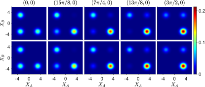
Figure 7: Dynamics for the single unitary rotation $U$ associated with the joint measurements of $S_{y}^{A}$ and $S_{z}^{B}$ by the superobservers is indistinguishable from that of $\rho_{mix,B}$: The notation is as for Figure 6. Top sequence: The system begins in $|\psi_{zz}\rangle_{FR}$ (Eq. (36)), and evolves according to $U_{A}^{-1}$ to the state $|\psi_{yz}\rangle_{FR}$ (Eq. (40)). Lower sequence: The system begins in $\rho_{mix,B}$ and evolves as for the top plots. The top and lower sequences are identical, which indicates consistency with weak macroscopic realism (refer text).

Similarly, after the appropriate reversal, the measurement $S_{y}$ at $B$ requires the evolution $U_{B}^{-1}(t_{b})|\psi_{zz}\rangle_{FR}$, which gives after a time $t_{b}=-\pi/2\equiv 3\pi/2$, the state $|\psi_{zy}\rangle_{FR}$. The dynamics for this measurement is plotted in Figure 8.

After the rotations to measure $S_{y}$ at both sites, the system is described by $U_{A}^{-1}U_{B}^{-1}|\psi_{zz}\rangle_{FR}$, as given by $|\psi_{yy}\rangle$ (Eq. (39)). The dynamics of these measurements in terms of the $Q$ function is plotted in Figure 9.

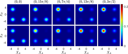
Figure 8: Dynamics for the single unitary rotation $U$ associated with the joint measurements of $S_{z}^{A}$ and $S_{y}^{B}$ by the superobservers is indistinguishable from that of $\rho_{mix,A}$, where Friend $B$’s measurement is not reversed: The notation is as for Figure 6. Top sequence: The system begins in $|\psi_{zz}\rangle_{FR}$ (Eq. (36)) and evolves according to $U_{B}^{-1}$ to the state $|\psi_{zy}\rangle_{FR}$ (Eq. (41)). Lower sequence: The system begins in $\rho_{mix,A}$ and evolves according to $U_{B}^{-1}$ as for the top plots. The two sequences are indistinguishable, indicating consistency with weak macroscopic realism (refer text).

VI.2.2 Comparison with the classical mixture $\rho_{zz}$: the perspective of the Friends

The mixture $\rho_{zz}$ (Eq. (50)) is the state formed from the perspective of the Friends, if the two Friends have both measured $\sigma_{z}$ at their locations e.g. by coupling to the meter. The $\rho_{zz}$ describes the statistical state of the system conditioned on both the Friends’ outcomes for their measurements of $\sigma_{z}$. The state is conditioned on the outcome $+1$ or $-1$ for the spins $S_{z}$ of the meter modes, denoted $Am$ and $Bm$ in (51), also found by integration of the full $Q$ function over the system and meter variables as explained in Section VI.A, to derive the result (54). Each meter mode is coupled to the system, so that the systems themselves can continue to evolve, conditioned on the outcome of the measurement on the meter. This evolution is given by that of $\rho_{zz}$.

The dynamics for $\rho_{zz}$ is plotted in Figure 6, below the dynamics for the superposition state $|\psi_{zz}\rangle_{FR}$. We see that the macroscopic difference between the predictions emerges over the timescales of the unitary interaction $U$ responsible for the measurement settings.

The state $\rho_{zz}$ is consistent with a model for which there is a definite predetermined outcome $\lambda_{z}^{A}$ and $\lambda_{z}^{B}$ for $\sigma_{z}$ in each Lab. The evolution for the system prepared in $\rho_{zz}$ is given as $\rho(t_{a},t_{b})=U_{A}^{-1}U_{B}^{-1}\rho_{zz}U_{A}U_{B}$, which satisfies a local realistic theory of the type considered by Bell, and as such does not violate the Bell-Wigner inequality. Hence, the paradox is not realised by $\rho_{zz}$. The superobservers must reverse the Friends’ measurements in order to restore the state $|\psi_{zz}\rangle_{FR}$. We note the violation of the Bell-Wigner inequality can be inferred, by performing measurements directly on $|\psi_{zz}\rangle_{FR}$, based on the assumption that a measurement of $S_{z}$ made by the superobservers would yield the same value as that of the Friends. It is clear that the predictions and dynamics displayed by the entangled state $|\psi_{zz}\rangle_{FR}$ are not compatible with the mixed state $\rho_{zz}$ (nor any state giving consistency with a local realistic theory, since such a state would not violate (42)).

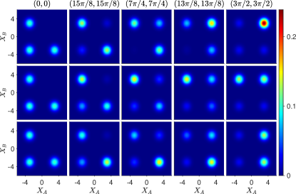
Figure 9: Dynamics for the two unitary rotations $U$ associated with the joint measurements of $S_{y}^{A}$ and $S_{y}^{B}$ by the superobservers. The notation is as for Figure 6. Top sequence: The system begins in $|\psi_{zz}\rangle_{FR}$ (Eq. (36)), and evolves according to $U_{A}^{-1}$ and $U_{B}^{-1}$ to the state $|\psi_{yy}\rangle_{FR}$ (Eq. (39)). Centre (lower) sequence: The system begins in $\rho_{mix,A}$ ($\rho_{mix,B}$) and evolves as for the top plots. The results for $|\psi_{zz}\rangle_{FR}$ diverge macroscopically from those of the mixed states over the dynamics, leading to a violation of the Wigner-Bell inequality for $|\psi_{zz}\rangle_{FR}$. This is not inconsistent with wMR: The wMR premise allows a failure of the macroscopic Bell-Locality premise where there are two rotations (refer Section V.B.2).

VI.2.3 Comparison with partial mixtures: conditioning on one Friend’s measurement

We now compare the evolution of $|\psi_{zz}\rangle_{FR}$ with that of partial mixtures obtained by conditioning on the outcomes of one Friend. This enables demonstration of the consistency with wMR, using the Result 6.B. (1).

First, we consider the dynamics for the measurements of $S_{z}^{B}$ and $S_{y}^{A}$, on the system prepared in the state $|\psi_{zz}\rangle_{FR}$. This dynamics creates $|\psi_{yz}\rangle_{FR}$. We compare with the mixture created if the spin measurement $\sigma_{z}^{B}$ made by the Friend in $L_{B}$ is not reversed. The Friend has coupled the meter $Bm$ to the system $B$, as in (51), and conditions all future measurements on the outcome for the meter being $+1$ or $-1$. The density operator for the combined system after a measurement of spin $\sigma_{z}$ at $B$ is the partial mixture

$$\rho_{mix,B} = \frac{1}{3}(|-\alpha\rangle\langle-\alpha|)(|\beta\rangle\langle\beta|)$$

$$+\frac{1}{3}\Bigl{\{}(|\alpha\rangle+i|-\alpha\rangle)(\langle\alpha|-i\langle-\alpha|)\Bigl{\}}(|-\beta\rangle\langle-\beta|).$$

Now we consider that a measurement $S_{y}^{A}$ is made on system $A$. This implies (after the appropriate reversal) the evolution according to $U_{A}^{-1}(t_{a})$, which is given in Figure 7 for both $|\psi_{zz}\rangle_{FR}$ and $\rho_{mix,B}$. The evolution of $\rho_{mix,B}$ is indistinguishable from that of $|\psi_{zz}\rangle_{FR}$.

We next consider the dynamics associated with the measurements of $S_{z}^{A}$ and $S_{y}^{B}$ on the system prepared in $|\psi_{zz}\rangle_{FR}$, which creates $|\psi_{zy}\rangle_{FR}$. For comparison, we also consider that the Friend at Lab A performs the measurement $\sigma_{z}^{A}$. The conditioning on the outcomes for the Friend’s measurement leaves the systems in the mixture

$$\rho_{mix,A} = \frac{1}{3}(|\alpha\rangle\langle\alpha|)(|-\beta\rangle\langle-\beta|)$$

$$+\frac{1}{3}(|-\alpha\rangle\langle-\alpha|)\Bigl{\{}\bigl{(}|\beta\rangle+i|-\beta\rangle\bigl{)}\bigr{(}\langle\beta|-i\langle-\beta|\bigl{)}\Bigl{\}}.$$

The dynamics associated with the measurement of $S_{y}^{B}$ involves the system evolving according to $U_{B}^{-1}(t_{b})$ is given in Figure 8. We see that the evolution for systems prepared in $|\psi_{zz}\rangle_{FR}$ is indistinguishable from that of systems prepared in $\rho_{mix,A}$.

Finally, we consider the dynamics where measurements of $S_{y}^{A}$ and $S_{y}^{B}$ are made on the system prepared in the state $|\psi_{zz}\rangle_{FR}$. Here, two local unitary rotations $U_{A}^{-1}(t_{a})$ and $U_{B}^{-1}(t_{b})$ are applied, to create the state $|\psi_{yy}\rangle_{FR}$, prepared in the pointer bases for the measurements $S_{y}^{A}$ and $S_{y}^{B}$. We compare this evolution with that of the system prepared in $\rho_{mix,A}$, or $\rho_{mix,B}$ (Figure 9). The evolution is macroscopically different in each case.

VI.2.4 Consistency with the weak macroscopic realism model

The predictions of quantum mechanics as given in Figures 7-9 reveal consistency with weak macroscopic realism (wMR). First, consider measurement of $\langle S_{y}^{A}S_{z}^{B}\rangle$. The evolution of $|\psi_{zz}\rangle_{FR}$ shown in Figure 7 is indistinguishable from that of $\rho_{mix,B}$. Hence, from Result 6.B.1, those results show consistency with wMR. After the interaction $U_{A}^{-1}$ in Lab $A$, the system is prepared in the appropriate basis, so that the final pointer measurement $S_{y}^{A}$ can be made by the superobserver. Hence, by Result 6.A, this state is also consistent with wMR. Similarly, prior to the dynamics $U_{A}^{-1}$ portrayed in the Figure 7, the superobservers perform the reversal of the Friends’ measurements. This does not change the preparation basis and, as argued in Section VI.A, a wMR model exists in which the pointer value $\lambda_{z}^{B,S}=\lambda_{z}^{B}$ is unchanged. We therefore conclude consistency with wMR.

The same arguments apply to the measurement of $\langle S_{z}^{A}S_{y}^{B}\rangle$. The evolution of $|\psi_{zz}\rangle_{FR}$ shown in Figure 8 is indistinguishable from that of $\rho_{mix,A}$. Hence, from Result 6.B.1, those results show consistency with wMR.

We claim a particular wMR model exists that replicates the quantum predictions of the $|\psi_{zz}\rangle_{FR}$, for the moments $\langle S_{z}^{A}S_{z}^{B}\rangle$, $\langle S_{z}^{A}S_{y}^{B}\rangle$ and $\langle S_{y}^{A}S_{z}^{B}\rangle$. At first glance the model seems not consistent, since for the different moments, we consider different mixed states ($\rho_{zz}$, $\rho_{mix,A}$ and $\rho_{mix,B}$) which are not compatible. In fact, we propose a more complete wMR model which includes local operations made by the superobservers. In the model, the system begins in $\rho_{zz}$ at the time $t_{2}$, and consistent with that mixed state, the results for both Friends’ measurements of $\sigma_{z}$ are known to the superobservers. Where the superobserver $A$ measures $S_{y}$ by applying $U_{A}^{-1}$, then in the model the superobserver $A$ first operates locally in Lab $A$ so that the overall system in $\rho_{zz}$ is transformed into $\rho_{mix,B}$. This local operation does not change the value of $\lambda_{z}^{B}$ in the model. Similarly, if superobserver $B$ measures $S_{y}$, then in the wMR model, a local operation is performed to change $\rho_{zz}$ into $\rho_{mix,A}$. For this model, wMR holds throughout the dynamics.

In summary, we have shown consistency of the quantum predictions of the Wigner friends paradoxes with both the wMR assertions. This was done using a particular wMR model, and showing compatibility with the predictions for $\langle S_{z}^{A}S_{z}^{B}\rangle$, $\langle S_{z}^{A}S_{y}^{B}\rangle$ and $\langle S_{y}^{A}S_{z}^{B}\rangle$. However, the particular wMR model used is a Bell-local realistic one, and does not describe the quantum dynamics for the measurements of $S_{y}$ at both Labs i.e. where there are two rotations $U$, one at $A$ and one at $B$. We see from Section V however that this does not imply the quantum predictions are inconsistent with the premise of wMR. The two assertions of wMR are not testable where there are unitary rotations at both sites (refer Figure 9), since both systems shift to a new pointer basis, so that the former pointer value $\lambda$ according to wMR no longer applies.

VII Conclusion and discussion

The motivation of this paper is to present a mapping between the microscopic Wigner friend paradoxes involving spin qubits and macroscopic versions involving macroscopically distinct spin states. In Section III, we provide such a mapping, where the macroscopically distinct states are two coherent states, $|\alpha\rangle$ and $|-\alpha\rangle$, $\alpha\rightarrow\infty.$ Unitary rotations $U$ determine which spin component is to measured and in a microscopic spin experiment correspond to Stern-Gerlach or polarizer-beam-splitter analyzers. In the macroscopic set-up, the $U$ are realised with nonlinear interactions.

The mapping motivates us to seek an interpretation for the paradoxes where macroscopic realism can be upheld. The extended Wigner-Friend paradoxes are based on very reasonable assumptions, including that of Locality, defined by Bell. We show in Section IV that the realisations of Brukner’s Bell-Wigner friend and the Frauchiger-Renner paradoxes each imply falsification of deterministic macroscopic (local) realism.

Motivated by that, we consider in Section V a more minimal definition of macroscopic realism, called weak macroscopic realism (wMR), which assigns realism to the system as it exists after the unitary rotation $U$ that determines the measurement setting. This establishes a predetermined value for the outcome of the pointer measurement that is to follow. The premise of wMR also establishes a locality for this value: the value is not affected by events at a spacelike-separated Lab. Careful examination shows that wMR does not imply a full Locality of the type postulated by Bell, which defines a realism for the system as it exists prior to the unitary dynamics $U$. In the remaining Sections VI-VII, we prove several Results, which confirm that the predictions of quantum mechanics for the paradoxes are consistent with wMR.

A feature of wMR is the definition of realism in a contextual sense. In the wMR model, the quantum state is not defined completely until the basis of preparation is specified. The basis of preparation for a particular state at a given time $t$ is defined as the basis such that the spin can be measured without a further unitary rotation $U$ that would give a change of measurement setting. The final measurement involves a sequence of operations such as amplification and detection, or coupling to meters. These operations are referred to as the final pointer stage of the measurement.

It is possible to define a similar contextual realism for the microscopic qubits. We refer to this as weak contextual realism (wR or wLR). The interpretations of the macroscopic paradoxes can be replicated in the microscopic versions, since there is a mapping between the two. The proofs of the Results in Sections IV-VI follow identically, for the spin $1/2$ system. This implies failure of deterministic local realism, and consistency with weak contextual realism. The violation of the Bell-CHSH and Brukner’s Bell-Wigner inequality is possible, because wLR does not imply the full Bell Locality assumption.

The results of this paper give insight into how the assumptions of Bell’s theorem may break down for quantum mechanics. We find the paradoxes arise only where the measurement setting is changed at both sites. This implies two unitary rotations. The unitary dynamics has been analyses using the $Q$ function. There is an effectively unobservable (as $\alpha\rightarrow\infty$) difference between the Q function of the macroscopic superposition and that of the corresponding mixture (the mixture giving consistency with the Bell-CHSH inequalities). The difference remains undetectable for the case where there is only a single rotation, which allows a predetermination of one of the measurement outcomes, so that wMR applies. However, where there are two rotations, the functions for the states evolving from the macroscopic superposition and the mixture become macroscopically different. This leads to macroscopic differences in the predictions, hence allowing the macroscopic paradox. This is the strangest mathematical paradox, because the final difference between the functions is macroscopic in the limit $\alpha\rightarrow\infty$, precisely the limit where the initial difference is increasingly negligible.

While we propose that wMR (and wLR) holds, we do not present a full wMR model consistent with all the quantum predictions of the paradox. The quantum predictions have been shown consistent with wMR only where the postulate wMR applies, which means where there has been a final measurement setting established. This leaves open the question of whether wMR is truly compatible with quantum mechanics, or whether it can be falsified. Arguments have been given elsewhere that there is inconsistency between wMR and the completeness of (standard) quantum mechanics (ghz-cat, ; manushan-bell-cat-lg, ; s-cat, ). This motivates examination of alternative theories, or theories which may give a more complete description of quantum mechanics (e.g. (DrummondReid2020, ; bohm, ; hall-cworlds, )), for consistency with wMR.

Finally, we consider a possible experiment. The microscopic superposition states can be mapped onto coherent-state superpositions using the methods of (cat-det-map, ; cat-bell-wang-1, ). The unitary rotations involving Kerr interactions have been realised in experiments creating cat states (cat-states-super-cond, ). The experiments could also be conducted using Greenberger-Horne-Zeilinger states and CNOT gates, as in (macro-realism-nori, ).

VIII Appendix

VIII.1 Examples of realisation of the Friend’s cat states

In this paper, we give three examples of a Wigner’s friend experiment where the initial spin system is a macroscopic one. The second example uses GHZ states and CNOT operations. Consider a large number of spin $1/2$ qubits. For Lab $A$, we select a set of $N+1$ qubits, choosing $|h\rangle=|\uparrow\rangle|\uparrow\rangle^{\otimes N}$ and $|t\rangle=|\downarrow\rangle|\downarrow\rangle^{\otimes N}$. Similar macroscopic qubits can be selected for Lab $B$. The qubits can be realised as orthogonally polarized photons in $N+1$ different modes. The coupling to the meters in the Labs links the systems to a larger set of $M$ qubits, so that $|H\rangle=|\uparrow\rangle|\uparrow\rangle^{\otimes N}|\uparrow\rangle^{\otimes M}$ and $|T\rangle=|\downarrow\rangle|\downarrow\rangle^{\otimes N}|\downarrow\rangle^{\otimes M}$. The unitary rotation $U_{x}$ or $U_{y}$ can be realised using CNOT gates. Suppose the system $A$ is created in $|H\rangle$. Then the photon of the first mode is passed through a beam splitter or polarizer-type interaction, to create

$$(|\uparrow\rangle+e^{i\varphi}|\downarrow\rangle)|\uparrow\rangle^{\otimes(N+M)}.$$ (71)

For each subsequent qubit, a CNOT operation is applied, which creates the Greenberger-Horne-Zeilinger (GHZ) state (ghz-amjp, ; mermin-inequality, ; omran-cats, ; ghz-1, )

$$|\uparrow\rangle|\uparrow\rangle^{\otimes(N+M)}+e^{i\varphi}|\downarrow\rangle|\downarrow\rangle^{\otimes(N+M)}.$$ (72)

The inclusion of a phase shift $\varphi$ at the first mode transformation allows either the $U_{x}$ or the $U_{y}$ to be realised. Such states have been used to experimentally demonstrate failure of macrorealism (macro-realism-nori, ), and have also been proposed for macroscopic tests of GHZ and Bohm-Einstein-Podolsky-Rosen paradoxes (ghz-cat, ), as well as for testing macroscopic Bell inequalities (manushan-bell-cat-lg, ).

The third example uses two-mode states and nonlinear interactions. The macroscopic qubits are two-mode number states, given by $|N\rangle_{1}|0\rangle_{2}$ and $|0\rangle_{1}|N\rangle_{2}$ where $|n\rangle_{i}$ is a number state for the mode $i$. These states for large $N$ are macroscopically distinct. The states were studied in (macro-bell-lg, ) and (ghz-cat, ), where it was shown that a nonlinear interaction $H_{nl}$ can create the macroscopic cat superposition according to $U_{x}$ and $U_{y}$ given by (21) and (22) (where we put $|H\rangle=|N\rangle|0\rangle_{2}$ and $|T\rangle=|0\rangle_{1}|N\rangle_{2}$). The transformations are not fully realised, but are sufficiently effective that violation of Bell inequalities are predicted.

VIII.2 Meter coupling

Let us consider the qubit $c|\uparrow\rangle+d|\downarrow\rangle$, where $c$ and $d$ are complex amplitudes. We couple the qubit system to a field mode prepared initially in a coherent state $|\gamma_{0}\rangle$. We consider the evolution under $H_{Am}$ where (spin-meter, ; Ilo-Okeke-byrnes-meter, ; blais-meter-model, ; spin-coupling, )

$$H_{Am}=\hbar G\sigma_{z}^{A}n_{c}^{A}.$$ (73)

Here $\sigma_{z}^{A}$ is the Pauli spin operator for the qubit system $A$, $n_{c}^{A}$ is the number operator for the meter mode $C$ in Lab A, and $G$ is a real constant. The solution for the final entangled state is

$$|\psi\rangle_{out} = e^{-iH_{d}t/\hbar}(c|\uparrow\rangle|\gamma_{0}\rangle+d|\downarrow\rangle|\gamma_{0}\rangle)$$

$$= c|\uparrow\rangle|\gamma\rangle+d|\downarrow\rangle|-\gamma\rangle$$

where we select $Gt=\pi/2$ and $\gamma=-i\gamma_{0}$.

VIII.3 Table of values for macroscopic realistic states

$\lambda_{zA}$	$\lambda_{zB}$	$\lambda_{yA}$	$\lambda_{yB}$	$P_{--|yy}$	$P_{-+|yy}$	$P_{+-|yy}$	$P_{++|yy}$	$P_{--|yz}$	$P_{--|zy}$
1	1	1	1	0	0	0	1	0	0
1	1	1	-1	0	0	1	0	0	0
1	1	-1	1	0	1	0	0	0	0
* 1	*1	*-1	*-1	*1	*0	*0	*0	*0	*0
1	-1	1	1	0	0	0	1	0	0
1	-1	1	-1	0	0	1	0	0	0
1	-1	-1	1	0	1	0	0	1	0
1	-1	-1	-1	1	0	0	0	1	0
-1	1	1	1	0	0	0	1	0	0
-1	1	1	-1	0	0	1	0	0	1
-1	1	-1	1	0	1	0	0	0	0
-1	1	-1	-1	1	0	0	0	0	1
-1	-1	1	1	0	0	0	1	0	0
-1	-1	1	-1	0	0	1	0	0	1
-1	-1	-1	1	0	1	0	0	1	0
-1	-1	-1	-1	1	0	0	0	1	1

References

- (1) E. P. Wigner, “Remarks on the mind-body question.”, In Symmetries and Reflections, 171184 (Indiana University Press, 1967).
- (2) C. Brukner, “A No-Go Theorem for Observer-Independent Facts”, Entropy 20, 350 (2018).
- (3) D. Frauchiger and R. Renner, “Quantum theory cannot consistently describe the use of itself.”, Nat. Commun. 9, 1 (2018).
- (4) M. Proietti, A. Pickston, F. Graffitti, P. Barrow, D. Kundys, C. Branciard, M. Ringbauer, and A. Fedrizzi, “Experimental test of local observer independence”, Science Adv. 5, 9 (2019).
- (5) A. Sudbery, “Single-World Theory of the Extended Wigner’s Friend Experiment”, Found. Phys. 47, 658 (2017).
- (6) R. Healey, “Quantum Theory and the Limits of Objectivity”, Found. Phys. 48, 1568 (2018).
- (7) M. Losada, R. Laura, and O. Lombardi, “Frauchiger-Renner argument and quantum histories”, Phys. Rev. A 100, 052114 (2019).
- (8) D. Lazarovici and M. Hubert, “How Quantum Mechanics can consistently describe the use of itself.”, Sci. Rep. 9, 470 (2019).
- (9) J. Bub, “In defense of a “single-world” interpretation of quantum mechanics”, Stud. Hist. Philos. Mod. Phys. 72, 251-255 (2020).
- (10) C. Elouard, P. Lewalle, S. K. Manikandan, S. Rogers, A. Frank, and A. N. Jordan, “Quantum erasing the memory of Wigner’s friend”, Quantum 5, 498 (2021).
- (11) A. Matzkin and D. Sokolovski, Wigner Friend scenarios with non-invasive weak measurements, Phys. Rev. A 102, 062204 (2020).
- (12) Dong Ding, Can Wang, Ying-Qiu He, Tong Hou, Ting Gao, and Feng-Li Yan, A scalable tripartite Wigner’s friend scenario, arXiv:2109.02298
- (13) K.- W. Bong, A. U.-Alarcón, F. Ghafari, Y.- C. Liang, N. Tischler, E. G. Cavalcanti, G. J. Pryde, and H. M. Wiseman, “A strong no-go theorem on the Wigner’s friend paradox”, Nature Physics 16, 1199–1205 (2020).
- (14) Matteo Lostaglio and Joseph Bowles, “The original Wigner’s friend paradox within a realist toy model”, Proc. R. Soc. A. 477, 20210273 (2021).
- (15) Marek Zukowski and Marcin Markiewicz, “Physics and Metaphysics of Wigner’s Friends: Even Performed Premeasurements Have No Results”, Phys. Rev. Lett. 126, 130402 (2021).
- (16) Veronika Baumann, Flavio Del Santo, Alexander R. H. Smith, Flaminia Giacomini, Esteban Castro-Ruiz, and Caslav Brukner, “Generalized probability rules from a timeless formulation of Wigner’s friend scenarios”, Quantum 5, 524 (2021).
- (17) Leonardo Castellani, “No Relation for Wigner’s Friend”, International Journal of Theoretical Physics 60, 2084 (2021).
- (18) Gijs Leegwater, “When Greenberger, Horne and Zeilinger Meet Wigner’s Friend” Foundations of Physics 52, 68 (2022).
- (19) C. Brukner, “Wigner’s friend and relational objectivity”, Nat. Rev. Phys. 4, 628 (2022).
- (20) E. Schrödinger, “The present status of quantum mechanics”, Naturwissenschaften 23, 823 (1935).
- (21) F. Fröwis, P. Sekatski, W. Dur, N. Gisin, and N. Sangouard, “Macroscopic quantum states: Measures, fragility, and implementations”, Rev Mod. Phys. 90, 025004 (2018).
- (22) A. Leggett and A. Garg, “Quantum mechanics versus macroscopic realism: is the flux there when nobody looks?” Phys. Rev. Lett. 54, 857 (1985).
- (23) C. Emary, N. Lambert, and F. Nori, Leggett-Garg inequalities, “Leggett–Garg inequalities”, Rep. Prog. Phys 77, 016001 (2014).
- (24) J. S. Bell, “Foundations of Quantum Mechanics”, ed B d’Espagnat (New York: Academic) pp171-81 (1971).
- (25) M. Thenabadu and M. D. Reid, “Bipartite Leggett-Garg and macroscopic Bell inequality violations using cat states: distinguishing weak and deterministic macroscopic realism”, Phys. Rev. A 105, 052207 (2022); arXiv:2012.14997; M. D. Reid and M. Thenabadu, “Weak versus deterministic macroscopic realism”, arXiv:2101.09476
- (26) Jesse Fulton, Run Yan Teh, and M. D. Reid, Argument for the incompleteness of quantum mechanics based on macroscopic and contextual realism: GHZ and Bohm-EPR paradoxes with cat states, arXiv:2208.01225
- (27) M. Thenabadu and M. D. Reid, “Macroscopic delayed-choice and retrocausality: quantum eraser, Leggett-Garg and dimension witness tests with cat states”, Phys. Rev. A 105, 062209 (2022).
- (28) P. Grangier, “Contextual Inferences, Nonlocality, and the Incompleteness of Quantum Mechanics”, Entropy 23, 1660 (2021) and references therein.
- (29) P. D. Drummond and M. D. Reid, “Retrocausal model of reality for quantum fields”, Phys. Rev. Research 2, 033266 (2020); P. D. Drummond and M. D. Reid, “Objective Quantum Fields, Retrocausality and Ontology”, Entropy 23, 749 (2021).
- (30) J. S. Bell, “On the Einstein-Podolsky-Rosen paradox”, Physics 1,195 (1964).
- (31) J. F. Clauser, M. A. Horne, A. Shimony, and R. A. Holt, “Proposed Experiment to Test Local Hidden-Variable Theories.” Phys. Rev. Lett. 23, 880 (1969).
- (32) J. F. Clauser and A. Shimony, “Bell’s theorem: experimental tests and implications”, Rep. Prog. Phys. 41, 1881 (1978).
- (33) N. Brunner, D. Cavalcanti, S. Pironio, V. Scarani, and S. Wehner, Bell nonlocality, Rev. Mod. Phys. 86, 419 (2014).
- (34) B. Yurke and D. Stoler, “Generating quantum mechanical superpositions of macroscopically distinguishable states via amplitude dispersion”, Phys. Rev. Lett. 57, 13 (1986).
- (35) G. Kirchmair et al., “Observation of the quantum state collapse and revival due to a single-photon Kerr effect”, Nature 495, 205 (2013).
- (36) B. Vlastakis, G. Kirchmair, Z. Leghtas, S. E. Nigg, L. Frunzio, S. M. Girvin, M. Mirrahimi, M. H. Devoret, and R. J. Schoelkopf, “Deterministically encoding quantum information using 100-photon schrödinger cat states”, Science 342, 607 (2013).
- (37) E. Wright, D. Walls, and J. Garrison, “Collapses and Revivals of Bose-Einstein Condensates Formed in Small Atomic Samples”, Phys. Rev. Lett. 77, 2158 (1996).
- (38) M. Greiner, O. Mandel, T. Hånsch, and I. Bloch, “Collapse and revival of the matter wave field of a Bose-Einstein condensate”, Nature 419, 51 (2002).
- (39) A. Ourjoumtsev, H. Jeong, R. Tualle-Brouri, and P. Grangier, “Generation of optical ‘Schrödinger cats’ from photon number states”, Nature 448,784 (2007).
- (40) M. Wolinsky and H. J. Carmichael, Quantum noise in the parametric oscillator: From squeezed states to coherent-state superpositions, Phys. Rev. Lett. 60 1836 (1988).
- (41) L. Krippner, W. J. Munro, and M. D. Reid, “Transient macroscopic quantum superposition states in degenerate parametric oscillation: Calculations in the large-quantum-noise limit using the positive p representation”, Phys. Rev. A 50, 4330 (1994).
- (42) E. E. Hach III and C. C. Gerry, “Generation of mixtures of schrödinger-cat states from a competitive two-photon process”, Phys. Rev. A 49, 490 (1994).
- (43) L. Gilles, B. M. Garraway, and P. L. Knight, “Generation of nonclassical light by dissipative two-photon processes”, Phys. Rev. A 49, 2785 (1994).
- (44) R. Y. Teh, S. Kiesewetter, Peter D. Drummond, and M. D. Reid “Creation, storage, and retrieval of an optomechanical cat state”, Physical Review A 98, 063814 (2018).
- (45) R. Y. Teh, F. X. Sun, R. E. S. Polkinghorne, Q. Y. He, Q. Gong, P. D. Drummond, and M. D. Reid, “Dynamics of transient cat states in degenerate parametric oscillation with and without nonlinear Kerr interactions”, Physical Review A 101, 043807 (2020).
- (46) M. Thenabadu, G-L. Cheng, T. L. H. Pham, L. V. Drummond, L. Rosales-Zárate, and M. D. Reid, “Testing macroscopic local realism using local nonlinear dynamics and time settings”, Phys. Rev. A 102, 022202 (2020).
- (47) M. Thenabadu and M. D. Reid, “Leggett-Garg tests of macrorealism for dynamical cat states evolving in a nonlinear medium”, Phys. Rev. A 99, 032125 (2019).
- (48) Zaki Leghtas, Gerhard Kirchmair, Brian Vlastakis, Michel H. Devoret, Robert J. Schoelkopf, and Mazyar Mirrahimi, “Deterministic protocol for mapping a qubit to coherent state superpositions in a cavity”, Phys. Rev. A 87, 042315 (2013).
- (49) C. Wang et al., A Schrödinger cat living in two boxes, Science 352, 1087 (2016).
- (50) Kôdi Husimi, “Some Formal Properties of the Density Matrix”, Proc. Phys. Math. Soc. Jpn. 22: 264 (1940).
- (51) D. M. Greenberger, M. Horne, and A. Zeilinger, “Going Beyond Bell’s Theorem, in Quantum Theory, and Conceptions of the Universe”, M. Kafatos, ed., Kluwer, Dordrecht, The Netherlands (1989), p. 69.
- (52) D. M. Greenberger, M. A. Horne, and A. Zeilinger, “Bell’s theorem without inequalities”, American Journal of Physics 58, 1131(1990).
- (53) N. D. Mermin, “Extreme Quantum Entanglement in a Superposition of Macroscopically Distinct States”, Phys. Rev. Lett. 65, 1838 (1990).
- (54) A. Omran, H. Levine, A. Keesling, G. Semeghini, T. T. Wang, S. Ebadi, H. Bernien, A. S. Zibrov, H. Pichler, S. Choi, et al., “Generation and manipulation of Schrödinger cat states in Rydberg atom arrays”, Science 365, 570 (2019).
- (55) H.-Y. Ku, N. Lambert, F.-J. Chan, C. Emary, Y.-N. Chen, and F. Nori, “Experimental test of non-macrorealistic cat states in the cloud”, npj Quantum Information 6, 98 (2020).
- (56) E. O. Ilo-Okeke and T. Byrnes, “Theory of Single-Shot Phase Contrast Imaging in Spinor Bose-Einstein Condensates” Phys. Rev. Lett. 112, 233602 (2014).
- (57) A. Wallraff, D. I. Schuster, A. Blais, L. Frunzio, R.- S. Huang, J. Majer, S. Kumar, S. M. Girvin and R. J. Schoelkopf, “Strong coupling of a single photon to a superconducting qubit using circuit quantum electrodynamics” Nature 431, 162 (2004).
- (58) L. Rosales-Zárate, B. Opanchuk, and M. D. Reid, “Weak measurements and quantum weak values for NOON states”, Phys. Rev. A 97, 032123 (2018).
- (59) A. Blais, R.- S. Huang, A. Wallraff, S. M. Girvin, and R. J. Schoelkopf, “Cavity quantum electrodynamics for superconducting electrical circuits: An architecture for quantum computation”, Phys. Rev. A 69, 062320 (2004).
- (60) D. Bohm, “A suggested interpretation of quantum theory in terms of “hidden” variables”, Phys. Rev. 85, pp 166-179 (1952).
- (61) M. J. Hall, D-A. Deckert, and H. J. Wiseman, “Quantum Phenonema modeled by interactions between Many Classical Worlds, Phys. Rev. X4, 041013 (2014).