main

Hamiltonian Transformation for Band Structure Calculations
Supplemental Material

S1 Decay properties of transformation

The basic idea of analyzing decay properties of a sparse matrix is approximating the transform function $f$ using polynomials and analyzing the expansion coefficients. Similar ideas were adopted to study the sparsity of density matrix [1, 2].

Consider a $m$-banded matrix $H$ such that:

1. $H$ is a Hermitian matrix.

2. The eigenvalue spectrum $\sigma(H)$ is contained in the interval $[-1,1]$.

3. There is an integer $m\geq 0$, so that $H_{ij}=0$ if $|i-j|>m$.

Although $H$ is limited to banded matrix here, our results in this section can be extended to general sparse matrices as long as we associate $H$ with a degree-limited and sparsely connected graph [2]. Therefore we can take the $m$-banded matrix $H$ as the SCF Hamiltonian.

We define the $k$th best approximation error of a transform function $f\in C[-1,1]$ as

$$E_{k}(f)=\inf\left\{\max_{-1\leq x\leq 1}|f(x)-p(x)|:p\in\mathcal{P}_{k}\right\},$$ (S1)

where $\mathcal{P}_{k}$ is the subspace of algebraic polynomials of degree at most $k$ in $C[-1,1]$. Let $i,j$ indices satisfy $mk<|i-j|\leq m(k+1)$, for any $p_{k}\in\mathcal{P}_{k}$, we have

$$\begin{split}\left|f(H)_{ij}\right|&=\left|[f(H)-p_{k}(H)]_{ij}\right|\\ &\leq\left\|f(H)-p_{k}(H)\right\|_{2}=\max_{x\in\sigma(H)}\left|f(x)-p_{k}(x)\right|\\ &\leq\max_{-1\leq x\leq 1}\left|f(x)-p_{k}(x)\right|\end{split}$$ (S2)

which means that

$$\left|f(H)_{ij}\right|\leq E_{k}(f).$$ (S3)

In Eq. S2 we have used

$$|A_{ij}|\leq\sqrt{\sum_{i}|A_{ij}|^{2}}=\left\|Ae_{j}\right\|_{2}\leq\sup_{x\neq\mathbf{0}}\frac{\left\|Ax\right\|_{2}}{\left\|x\right\|_{2}}=\left\|A\right\|_{2}.$$ (S4)

The exact expression of the optimal $p_{k}$ is unknown. While we can approximately achieve $E_{k}(f)$ using Chebyshev polynomials. Approximation theory guarantees that Chebyshev polynomials are nearly optimal. The error bounds for the Chebyshev series are known for smooth functions [3, 4]. Here we calculate exact error bounds for some specific functions.

The expression of $f$ in the Chebyshev polynomials basis sets is

$$f(x)=\frac{1}{2}\alpha_{0}+\sum_{l=1}^{\infty}\alpha_{l}T_{l}(x),$$ (S5)

$$\alpha_{l}=\frac{2}{\pi}\int_{0}^{\pi}f(\cos\theta)\cos{l\theta}d\theta,$$ (S6)

where $T_{l}(x)$ is the $l$th Chebyshev polynomial of the first kind. As a result, the decay properties of $f(H)$ can be estimated using

$$\begin{split}&|f(H)_{ij}|\leq E_{k}(f)\leq\left\|\sum_{l=k+1}^{\infty}\alpha_{l}T_{l}(x)\right\|_{x\in[-1,1]}\\ =&\frac{2}{\pi}\left\|\sum_{l=k+1}^{\infty}\cos{l\theta}\int_{0}^{\pi}f(\cos t)\cos{lt}\ dt\right\|_{\theta\in[0,\pi]}.\end{split}$$ (S7)

In numerical calculations, Eq. S5 is adopted to simplify $\sum_{k+1}^{\infty}$ to $\sum_{1}^{k}$.

S2 Analytical solution of decay properties

Here we provide an analytical solution of the decay properties of the $m$-banded matrix $H$ with a simple transform function

$$f_{n}(x)=\begin{cases}-(-x)^{n}&x\leq 0\\ 0&x>0\end{cases},$$ (S8)

where $n\in{\mathbb{N}}$.

According to Eq. S6,

$$\alpha_{l,n}=-\frac{2}{\pi}\int_{\frac{\pi}{2}}^{\pi}(-\cos\theta)^{n}\cos{l\theta}d\theta.$$ (S9)

The closed-form of $\alpha_{l,n}$ is quite complicated, but it turns simpler when $l>n$. In this case, it is easy to prove

$$\alpha_{l,0}=\frac{2\sin(\frac{l\pi}{2})}{\pi l},$$ (S10)

$$\alpha_{l,1}=\frac{2\cos(\frac{l\pi}{2})}{\pi(l^{2}-1)},$$ (S11)

and the recurrence relation

$$\alpha_{l,n}=\frac{-n(n-1)\alpha_{l,n-2}}{(l+n)(l-n)},$$ (S12)

using integration by parts. Thus

$$\alpha_{l,n}=\frac{2n!\sin(\frac{(l+n)\pi}{2})}{\pi\prod_{s=0}^{n}(l-n+2s)}\ (l>n).$$ (S13)

We have

$$\begin{split}&E_{k}(f_{n})\leq\left\|\sum_{l=k+1}^{\infty}\alpha_{l,n}T_{l}(x)\right\|\\ =&\frac{2n!}{\pi}\left\|\sum_{l=k-n+1}^{\infty}\frac{\sin(\frac{(l+2n)\pi}{2})\cos(l+n)\theta}{\prod_{s=0}^{n}(l+2s)}\right\|\\ =&\frac{2n!}{\pi}\left\|\sum_{l=\lfloor\frac{k-n+1}{2}\rfloor}^{\infty}\frac{\sin(\frac{(2l+2n+1)\pi}{2})\cos(2l+n+1)\theta}{\prod_{s=0}^{n}(2l+2s+1)}\right\|\\ =&\frac{2n!}{\pi}\left\|\sum_{l=l_{0}}^{\infty}\frac{(-1)^{l+n}\cos(2l+n+1)\theta}{\prod_{s=0}^{n}(2l+2s+1)}\right\|,\end{split}$$ (S14)

where $l_{0}=\lfloor\frac{k-n+1}{2}\rfloor$, $\lfloor x\rfloor$ is floor function and $k\geq n$.

We can rewrite Eq. S14 using special function:

$$\begin{split}&\frac{2n!}{\pi}\left\|\Re\left[\sum_{l=l_{0}}^{\infty}\frac{(-1)^{l+n}e^{\mathord{\mathrm{i}}(2l+n+1)\theta}}{\prod_{s=0}^{n}(2l+2s+1)}\right]\right\|\\ =&\frac{n!}{2^{n}\pi}\frac{\Gamma(l_{0}+\frac{1}{2})}{\Gamma(l_{0}+n+\frac{3}{2})}\left\|\Re\left[e^{\mathord{\mathrm{i}}(2l_{0}+n+1)\theta}F(1,l_{0}+\frac{1}{2},l_{0}+n+\frac{3}{2};-e^{2\mathord{\mathrm{i}}\theta})\right]\right\|\\ \leq&\frac{n!\Gamma(l_{0}+\frac{1}{2})}{2^{n}\pi\Gamma(l_{0}+n+\frac{3}{2})}\left\|\left|F(1,l_{0}+\frac{1}{2},l_{0}+n+\frac{3}{2};-e^{2\mathord{\mathrm{i}}\theta})\right|\right\|,\end{split}$$ (S15)

where $\Re$ is real part, $\Gamma$ is Gamma function, and $F$ is hypergeometric function defined as

$$F(a,b,c;z)=\sum_{k=0}^{\infty}\frac{(a)_{k}(b)_{k}}{(c)_{k}}\frac{z^{k}}{k!},$$ (S16)

$$(a)_{k}=\frac{\Gamma(a+k)}{\Gamma(a)}.$$ (S17)

It is clear to see that

$$\begin{split}\left|F(1,l_{0}+\frac{1}{2},l_{0}+n+\frac{3}{2};-e^{2\mathord{\mathrm{i}}\theta})\right|=\left|\sum_{k=0}^{\infty}\frac{(l_{0}+\frac{1}{2})_{k}}{(l_{0}+n+\frac{3}{2})_{k}}(-e^{2\mathord{\mathrm{i}}\theta})^{k}\right|\end{split}$$ (S18)

reaches the maximum when $\theta=\frac{\pi}{2}$ and all terms of the sum are positive. Thus we have

$$\begin{split}&|f_{n}(H)_{ij}|\leq E_{k}(f_{n})\\ \leq&\frac{n!\Gamma(l_{0}+\frac{1}{2})}{2^{n}\pi\Gamma(l_{0}+n+\frac{3}{2})}F(1,l_{0}+\frac{1}{2},l_{0}+n+\frac{3}{2};1)\\ =&\frac{n!\Gamma(l_{0}+\frac{1}{2})}{2^{n}\pi\Gamma(l_{0}+n+\frac{3}{2})}\frac{2l_{0}+2n+1}{2n}\\ =&\frac{n!}{\pi n\prod_{s=0}^{n-1}(2l_{0}+2s+1)}\\ \leq&\frac{(n-1)!}{\pi(k-n+1)^{n}}\ (k\geq n>0).\end{split}$$ (S19)

Recall that $mk<|i-j|\leq m(k+1)$, for sufficient large $|i-j|$, $|f_{n}(H)_{ij}|$ decays at least polynomially with a rate $\sim|i-j|^{-n}$. Note that $f_{n}$ is $(n-1)$-differentiable.

S3 Numerical solution of decay properties

With the help of numerical methods, we could study a group of more complicated transform functions:

$$f_{a,n}(x)=\begin{cases}x+a/2&x\leq-a\\ \frac{\frac{2a(e^{-\frac{n^{2}}{4}}-e^{-\frac{n^{2}(2x+a)^{2}}{4a^{2}}})}{\sqrt{\pi}n}+(2x+a)\left(\text{erf}\left(\frac{n}{2}\right)-\text{erf}\left(n\left(\frac{x}{a}+\frac{1}{2}\right)\right)\right)}{4\text{erf}\left(\frac{n}{2}\right)}&-a<x\leq 0\\ 0&x>0\end{cases},$$ (S20)

where erf(x) is error function.

The decay properties are calculated by

$$\begin{split}&|f_{a,n}(H)_{ij}|\leq E_{k}(f_{a,n})\\ \leq&\frac{2}{\pi}\left\|\sum_{l=k+1}^{\infty}\cos{l\theta}\int_{\frac{\pi}{2}}^{\pi}f_{a,n}(\cos t)\cos{lt}\ dt\right\|_{\theta\in[0,\pi]}\\ =&c_{a,n}F[f_{a,n},k],\end{split}$$ (S21)

where $c_{a,n}$ is a factor normalizes $F[f_{a,n},0]$ to 1. Similar to $f_{n}$ in Eq. S8, $f_{a,n}$ also becomes smoother for larger $n$. We choose $a=1$, $a=\frac{1}{2}$ and $a=\frac{1}{4}$, respectively, and the results are plotted in Fig. S1. Calculations are performed using Mathematica [5].

Fig. S1: The decay properties of transformed $m$-banded matrix $H$, $|f_{a,n}(H)_{ij}|\leq c_{a,n}F[f_{a,n},k]$, $mk<|i-j|\leq m(k+1)$, $c_{a,n}$ is a factor normalizes $F[f_{a,n},0]$ to 1. (a), (b) and (c) corresponds to $a=1$, $a=\frac{1}{2}$ and $a=\frac{1}{4}$, respectively. Black dashed lines are $F[f_{0,n},k]$.

In Fig. S1, the black dashed lines are $F[f_{0,n},k]$, and colored solid lines are $F[f_{a,n},k]$ with $a\neq 0$, we can see that $H$ decays much faster after transformation. Comparing Fig. S1(a), (b) and (c), their images are similar after scaling, but the larger $a$ makes $F[f_{a,n},k]$ decreases faster. When $k$ is sufficient large, larger $n$ makes $F[f_{a,n},k]$ smoother and makes $H$ decreases faster, which is in consistent with the results of the analytical case. However, when $k$ is small, smaller $n$ makes $H$ decreases faster.

S4 Projection of WFs increases decay radius

All our discussions in this section are in the infinite large supercell instead of unit cell or finite supercell, and only isotropic systems are considered for simplicity. Suppose a periodic system with Born–von Karman boundary condition, its Hamiltonian is

$$H({\mathbf{r}},{\mathbf{r}}^{\prime}),\quad{\mathbf{r}},{\mathbf{r}}^{\prime}\in\Omega^{l},$$ (S22)

where $\Omega^{l}$ is supercell, and

$$\lim_{|{\mathbf{r}}-{\mathbf{r}}^{\prime}|\to\infty}H({\mathbf{r}},{\mathbf{r}}^{\prime})=0.$$ (S23)

In the Wannier interpolation, we cannot utilize $H$ directly since its multiplications with eigenvectors are quite time consuming. In practice, only $N_{b}N_{k}$ eigenvalues $\varepsilon_{i{\mathbf{k}}}$ and eigenvectors $\psi_{i{\mathbf{k}}}$ are available, where $N_{b}$ is the number of bands, $N_{k}$ is the number of SCF ${\mathbf{k}}$-points. The Hamiltonian for Wannier interpolation is

$$H_{1}({\mathbf{r}},{\mathbf{r}}^{\prime})=\sum_{i=1}^{N_{b}}\sum_{{\mathbf{k}}=1}^{N_{k}}\varepsilon_{i{\mathbf{k}}}\psi_{i{\mathbf{k}}}({\mathbf{r}})\psi_{i{\mathbf{k}}}^{*}({\mathbf{r}}^{\prime}).$$ (S24)

We choose a threshold $t>0$ and define the decay radius $r_{0}$ of $H({\mathbf{r}},{\mathbf{r}}^{\prime})$ as

$$r_{0}=\sup\left\{|{\mathbf{r}}-{\mathbf{r}}^{\prime}|:\left|H({\mathbf{r}},{\mathbf{r}}^{\prime})\right|\geq t\right\},$$ (S25)

and define the decay radius of $H_{1}$ as $r_{1}$ similarly.

The localization property of $H_{1}$ is worse than $H$, which means $r_{1}>r_{0}$. For the disentangled bands, $H_{1}({\mathbf{r}},{\mathbf{r}}^{\prime})$ usually decays rapidly, the difference between $r_{0}$ and $r_{1}$ can be ignored. However, for the entangled bands, $r_{1}$ is usually significantly larger than $r_{0}$. Of course, we can define a new objective function that describes the locality of Hamiltonian, then localize Hamiltonian with iterative methods to obtain the “maximally localized Hamiltonian”. However, the size of Hamiltonian is large, and localizing the Hamiltonian is much more expensive than localizing Wannier functions.

Wannier interpolation projects $H_{1}$ to the subspace spanned by $\phi_{i{\mathbf{k}}}$:

$$(H_{\mathbf{k}}^{\text{wan}})_{mn} =\sum_{i,j=1}^{N_{b}}\int_{\Omega^{l}\times\Omega^{l}}d{\mathbf{r}}d{\mathbf{r}}^{\prime}V_{{\mathbf{k}},im}^{\dagger}\psi_{i{\mathbf{k}}}^{*}({\mathbf{r}})H_{1}({\mathbf{r}},{\mathbf{r}}^{\prime})\psi_{j{\mathbf{k}}}({\mathbf{r}}^{\prime})V_{{\mathbf{k}},jn}$$

$$=\int_{\Omega^{l}\times\Omega^{l}}d{\mathbf{r}}d{\mathbf{r}}^{\prime}\phi_{m{\mathbf{k}}}^{*}({\mathbf{r}})H_{1}({\mathbf{r}},{\mathbf{r}}^{\prime})\phi_{n{\mathbf{k}}}({\mathbf{r}}^{\prime})$$ (S26a)

$$=\sum_{i=1}^{N_{b}}\varepsilon_{i{\mathbf{k}}}V_{{\mathbf{k}},im}^{\dagger}V_{{\mathbf{k}},in},$$ (S26b)

where $1\leq m,n\leq N_{w}$, $N_{w}$ ($\leq N_{b}$) is the number of Wannier bands, $V_{{\mathbf{k}},im}$ is a $k$-dependent $N_{b}\times N_{w}$ gauge matrix combines disentanglement and maximal localization, $\phi_{m{\mathbf{k}}}({\mathbf{r}})$ is the Wannier-gauge Bloch states defined as

$$\phi_{m{\mathbf{k}}}({\mathbf{r}})=\sum_{i=1}^{N_{b}}\psi_{i{\mathbf{k}}}({\mathbf{r}})V_{{\mathbf{k}},im}.$$ (S27)

Eq. S26a and S26b are two equivalent expressions of $H_{\mathbf{k}}^{\text{wan}}$. Eq. S26a is used in our following analysis, and Eq. S26b is the actual formula adopted in the Wannier interpolation.

Considering the projected Hamiltonian in real space,

$$(H_{\mathbf{R}}^{\text{wan}})_{mn}=\mathcal{F}^{-1}(H_{\mathbf{k}}^{\text{wan}})_{mn}=\frac{1}{\sqrt{N_{k}}}\int_{\Omega^{l}\times\Omega^{l}}d{\mathbf{r}}d{\mathbf{r}}^{\prime}\left(\phi_{m(-{\mathbf{R}})}^{*}({\mathbf{r}})\circledast\phi_{n{\mathbf{R}}}({\mathbf{r}}^{\prime})\right)H_{1}({\mathbf{r}},{\mathbf{r}}^{\prime}),$$ (S28)

where $\mathcal{F}^{-1}$ is inverse Fourier transform on the Bravais lattice vector ${\mathbf{R}}$ (not on ${\mathbf{r}}$), $\circledast$ is convolution along ${\mathbf{R}}$. $\phi_{m{\mathbf{R}}}({\mathbf{r}})$ is Wannier function which satisfies

$$\phi_{m{\mathbf{R}}}({\mathbf{r}})=\mathcal{F}^{-1}(\phi_{m{\mathbf{k}}}({\mathbf{r}}))=\frac{1}{\sqrt{N_{\mathbf{k}}}}\sum_{\mathbf{k}}e^{\mathord{\mathrm{i}}{\mathbf{k}}\cdot{\mathbf{R}}}\phi_{m{\mathbf{k}}}({\mathbf{r}}),\quad{\mathbf{r}}\in\Omega^{l}.$$ (S29)

The last equality of Eq. S28 can be proven by

$$\begin{split}&\frac{1}{\sqrt{N_{k}}}\int_{\Omega^{l}\times\Omega^{l}}d{\mathbf{r}}d{\mathbf{r}}^{\prime}\left(\phi_{m(-{\mathbf{R}})}^{*}({\mathbf{r}})\circledast\phi_{n{\mathbf{R}}}({\mathbf{r}}^{\prime})\right)H_{1}({\mathbf{r}},{\mathbf{r}}^{\prime})\\ =&\frac{1}{\sqrt{N_{k}}}\int_{\Omega^{l}\times\Omega^{l}}d{\mathbf{r}}d{\mathbf{r}}^{\prime}\sum_{{\mathbf{R}}_{1}}\phi_{m(-{\mathbf{R}}_{1})}^{*}({\mathbf{r}})\phi_{n({\mathbf{R}}-{\mathbf{R}}_{1})}({\mathbf{r}}^{\prime})H_{1}({\mathbf{r}},{\mathbf{r}}^{\prime})\\ =&\frac{1}{N_{k}^{3/2}}\int_{\Omega^{l}\times\Omega^{l}}d{\mathbf{r}}d{\mathbf{r}}^{\prime}\sum_{{\mathbf{R}}_{1},{\mathbf{k}}_{1},{\mathbf{k}}}\phi_{m{\mathbf{k}}_{1}}^{*}({\mathbf{r}})e^{\mathord{\mathrm{i}}{\mathbf{k}}_{1}\cdot{\mathbf{R}}_{1}}\phi_{n{\mathbf{k}}}({\mathbf{r}}^{\prime})e^{\mathord{\mathrm{i}}{\mathbf{k}}\cdot({\mathbf{R}}-{\mathbf{R}}_{1})}H_{1}({\mathbf{r}},{\mathbf{r}}^{\prime})\\ =&\frac{1}{\sqrt{N_{k}}}\sum_{{\mathbf{k}}}\int_{\Omega^{l}\times\Omega^{l}}d{\mathbf{r}}d{\mathbf{r}}^{\prime}\phi_{m{\mathbf{k}}}^{*}({\mathbf{r}})H_{1}({\mathbf{r}},{\mathbf{r}}^{\prime})\phi_{n{\mathbf{k}}}({\mathbf{r}}^{\prime})e^{\mathord{\mathrm{i}}{\mathbf{k}}\cdot{\mathbf{R}}}\\ =&\mathcal{F}^{-1}(H_{\mathbf{k}}^{\text{wan}})_{mn}.\end{split}$$ (S30)

We define the decay radius $r_{w}$ of Wannier function $\phi_{m{\mathbf{R}}}({\mathbf{r}})$ as

$$r_{w}=\sup\left\{|{\mathbf{r}}|:\left|\phi_{m\mathbf{0}}({\mathbf{r}})\right|\geq t\right\},$$ (S31)

and define the truncated $\tilde{H}_{1}$ and $\tilde{\phi}$ as

$$\tilde{H}_{1}({\mathbf{r}},{\mathbf{r}}^{\prime})=\begin{cases}H_{1}({\mathbf{r}},{\mathbf{r}}^{\prime})&|{\mathbf{r}}-{\mathbf{r}}^{\prime}|\leq r_{1}\\ 0&|{\mathbf{r}}-{\mathbf{r}}^{\prime}|>r_{1}\end{cases},$$ (S32)

$$\tilde{\phi}({\mathbf{r}})=\begin{cases}\phi({\mathbf{r}})&|{\mathbf{r}}|\leq r_{w}\\ 0&|{\mathbf{r}}|>r_{w}\end{cases}.$$ (S33)

Thus

$$(H_{\mathbf{R}}^{\text{wan}})_{mn}=(\tilde{H}_{\mathbf{R}}^{\text{wan}})_{mn}+\mathcal{O}(t)=\frac{1}{\sqrt{N_{k}}}\int_{\Omega^{l}\times\Omega^{l}}d{\mathbf{r}}d{\mathbf{r}}^{\prime}\left(\tilde{\phi}_{m(-{\mathbf{R}})}^{*}({\mathbf{r}})\circledast\tilde{\phi}_{n{\mathbf{R}}}({\mathbf{r}}^{\prime})\right)\tilde{H}_{1}({\mathbf{r}},{\mathbf{r}}^{\prime})+\mathcal{O}(t).$$ (S34)

$\tilde{H}_{\mathbf{R}}^{\text{wan}}\neq 0$ requires

$$\begin{cases}|{\mathbf{r}}-{\mathbf{r}}^{\prime}|\leq r_{1}\\ |{\mathbf{r}}+{\mathbf{R}}_{1}|\leq r_{w}\\ |{\mathbf{r}}^{\prime}-{\mathbf{R}}+{\mathbf{R}}_{1}|\leq r_{w},\end{cases}$$ (S35)

which means that

$$|{\mathbf{R}}|\leq r_{1}+2r_{w}.$$ (S36)

Strictly speaking, we only provide an upper bound here and cannot guarantee the upper bound is always reached. The convolution of two functions may have a smaller decay radius if their spectra have non-intersecting supports. However, the supports of Hamiltonian and Wannier functions in reciprocal space usually take up the whole cut-off sphere and coincide with each other. We can expect $H_{\mathbf{R}}^{\text{wan}}$ have a decay radius of $r_{1}+2r_{w}$ in most cases.

S5 Changing basis sets

To reduce the size of basis sets, we expand the original orbitals $\psi_{i{\mathbf{k}}}$ in the auxiliary basis $Q_{\mu}({\mathbf{r}})$:

$$\psi_{i{\mathbf{k}}}({\mathbf{r}})=\sum_{\mu=1}^{N_{\mu}}Q_{\mu}({\mathbf{r}})C_{{i{\mathbf{k}}}\mu}.$$ (S37)

Here $\psi_{i{\mathbf{k}}}({\mathbf{r}})=e^{\mathord{\mathrm{i}}{\mathbf{k}}\cdot{\mathbf{r}}}u_{i{\mathbf{k}}}({\mathbf{r}})$, but ${\mathbf{r}}$ is restricted to the unit cell with ${\mathbf{R}}=\mathbf{0}$. Noting that $Q_{\mu}({\mathbf{r}})$ is independent of ${\mathbf{k}}$, orbitals at all ${\mathbf{k}}$-points share the same auxiliary basis, and changing to this basis sets will not affect the decay radius of Hamiltonian.

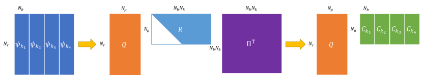
Fig. S2: Graphical representation of changing basis sets through QRCP. Equivalent to Eq. S38.

Changing basis sets is performed by QR factorization with column pivoting (QRCP) [6]:

$$\Psi\Pi=QR\ \Leftrightarrow\ \Psi=QR\Pi^{\mathsf{T}}=QC.$$ (S38)

Fig. S2 is the graphical representation of Eq. S38, where $\Psi$ is a $N_{r}\times N_{k}N_{b}$ matrix obtained by concatenating all $\psi_{i{\mathbf{k}}}$ along the $N_{b}$ dimension, $Q$ is a $N_{r}\times N_{\mu}$ matrix whose columns are orthonormal, $R$ is an upper triangular matrix, and $\Pi$ is a permutation matrix. $\Pi$ permutes columns of $\psi$ such that the magnitudes of the diagonal elements of $R$ are in a nonincreasing ordering. The magnitudes of diagonal elements of $R$ indicate the importance of the corresponding rows of $R$ and columns of $Q$. We denote $N_{\mu}$ as the number of diagonal elements of $R$ larger than a threshold. $N_{\mu}$ is the numerical rank of space spanned by the lowest $N_{b}$ orbitals of all ${\mathbf{k}}$-points; it will tend to be a constant multiple of $N_{b}$ even if $N_{k}$ approaches infinity.

The Hamiltonian can be written as

$$H_{\mathbf{k}}({\mathbf{r}},{\mathbf{r}}^{\prime})=\sum_{\mu\nu}Q_{\mu}({\mathbf{r}})M_{\mathbf{k}}(\mu,\nu)Q_{\nu}^{*}({\mathbf{r}}^{\prime}),$$ (S39)

$$M_{\mathbf{k}}(\mu,\nu)=\sum_{i=1}^{N_{b}}\varepsilon_{i{\mathbf{k}}}C_{{i{\mathbf{k}}}\mu}C_{{i{\mathbf{k}}}\nu}^{*}.$$ (S40)

Considering the Fourier interpolation of Eq. S39,

$$\begin{split}H_{\mathbf{q}}({\mathbf{r}},{\mathbf{r}}^{\prime})&=\frac{1}{N_{k}}\sum_{{\mathbf{k}},{\mathbf{R}}}H_{\mathbf{k}}({\mathbf{r}},{\mathbf{r}}^{\prime})e^{\mathord{\mathrm{i}}({\mathbf{k}}-{\mathbf{q}}){\mathbf{R}}}\\ &=\sum_{\mu\nu}Q_{\mu}({\mathbf{r}})(\frac{1}{N_{k}}\sum_{{\mathbf{k}},{\mathbf{R}}}M_{\mathbf{k}}(\mu,\nu)e^{\mathord{\mathrm{i}}({\mathbf{k}}-{\mathbf{q}}){\mathbf{R}}})Q_{\nu}^{*}({\mathbf{r}}^{\prime})\\ &=\sum_{\mu\nu}Q_{\mu}({\mathbf{r}})M_{\mathbf{q}}(\mu,\nu)Q_{\nu}^{*}({\mathbf{r}}^{\prime}).\end{split}$$ (S41)

We can see the Fourier interpolation of a $N_{r}\times N_{r}$ matrix $H_{\mathbf{k}}({\mathbf{r}},{\mathbf{r}}^{\prime})$ is simplified to that of a $N_{\mu}\times N_{\mu}$ matrix $M_{\mathbf{k}}(\mu,\nu)$.

When the projector augmented wave method (PAW) or ultrasoft pseudopotentials are adopted, orbitals are nonorthogonal. Hamiltonian transformation method is still available as long as we replace $\psi_{\mathbf{k}}$ with $S^{\frac{1}{2}}\psi_{\mathbf{k}}$, where $S$ is the overlap matrix independent of orbitals and ${\mathbf{k}}$-points.

S6 The size of $N_{\mu}$

We perform some tests to study the relationship between $N_{\mu}$, $N_{r}$, $N_{b}$ and $N_{w}$. The system is silicon, generalized gradient approximation of Perdew-Burke-Ernzerhof (GGA-PBE) [7] functional is adopted, cutoff energy is 100 Ry. $n=3$ for transform function. The SCF FFT grid is $48\times 48\times 48$, in HT we adopt a coarse grid for orbitals, which is $25\times 25\times 25$, so $N_{r}=15625$. Here we do not perform WI, but the mean absolute error (MAE) considers the lowest 8 bands, it is equivalent to $N_{w}=8$.

We sort the diagonal values of $R$ in QRCP according to their absolute values, assuming the largest as 1, and ignore those smaller than $\epsilon_{t}$. The relationship between $\epsilon_{t}$, $N_{\mu}$, $N_{k}$ and MAE is shown in Fig. S3. If $\epsilon_{t}$ is fixed, $N_{\mu}$ tends to a constant when $N_{k}$ is large enough. When $N_{k}=27$, $N_{\mu}\approx 90$ could reach the maximum accuracy; when $N_{k}=1000$, $N_{\mu}\approx 225$ could reach the maximum accuracy. In this case, we have $N_{\mu}\approx 0.01N_{r}$ and $N_{\mu}\approx 20N_{w}$. In the QRCP procedure we consider 14 bands, i.e. $N_{b}=14$. If $N_{b}$ is reduced to 10, $N_{\mu}$ can be smaller. $N_{\mu}/N_{r}$ is also dependent of cutoff energy, the higher cutoff energy corresponds to smaller $N_{\mu}/N_{r}$. From our experience, $N_{\mu}/N_{r}\approx 0.01\sim 0.1$ in most cases.

Fig. S3: The relationship between $\epsilon_{t}$, $N_{\mu}$, $N_{k}$ and MAE.

S7 Computational methods

Our Hamiltonian transformation method is implemented in Quantum ESPRESSO [8, 9, 10], DFT calculations are performed by Quantum ESPRESSO. The quasi-particle energy in the GW level is calculated by BerkeleyGW [11, 12]. Wannier interpolations are performed by Wannier90 [13].

We adopt optimized norm-conserving Vanderbilt (ONCV) [14] pseudopotential in all calculations. Selected columns of the density matrix (SCDM) method [15, 16, 17] is used for Wannier interpolation if not specified otherwise. In Fig. LABEL:fig:band(a), the unit cell of silicon contains two silicon atoms, ${\mathbf{k}}$-point mesh is $5\times 5\times 5$, cutoff energy is 25 Ry, and we use sp³ projection for Wannier interpolation. In Fig. LABEL:fig:band(b), ${\mathbf{k}}$-point mesh is $11\times 11\times 1$, cutoff energy is 50 Ry, SCDM-$\mu$ is 2, SCDM-$\sigma$ is 1. In Fig. LABEL:fig:band(c), generalized gradient approximation of Perdew-Burke-Ernzerhof (GGA-PBE) [7] functional is adopted, cutoff energy is 100 Ry, SCDM-$\mu$ is 10, SCDM-$\sigma$ is 2. The mean absolute error (MAE) calculation considers ${\mathbf{k}}$-points between $\Gamma$ and X. In Fig. LABEL:fig:band(d), GGA-PBE functional is adopted, cutoff energy is 10 Ry.

S8 Time complexity

The theoretical time complexity of Hamiltonian transformation is shown in Table S1. Its computational bottleneck lies in randomized QRCP and iterative diagonalization, which have time complexities of $\mathcal{O}(N_{\mu}^{2}(N_{r}+N_{b}N_{k}))$ and $\mathcal{O}(N_{\mu}^{2}N_{b}N_{q})$, respectively. At present, randomized QRCP, NUFFT, and iterative diagonalization are not yet implemented in our code. They are temporarily replaced by QRCP, matrix multiplication, and direct diagonalization, respectively.

If we assume $N_{r},N_{\mu},N_{b}$ proportion to the number of electrons $N_{e}$, and $N_{q}$ is constant, the total time complexity of Hamiltonian transformation is $\mathcal{O}(N_{e}^{3}N_{k}\log(N_{k}))$. Here the $\log(N_{k})$ term comes from fast Fourier transform, which has a small preconstant and is neglectable in most cases.

Table S1: The theoretical time complexity of Hamiltonian transformation. $N_{r}$ is the number of real space grids, $N_{\mu}$ is the size of new basis sets, $N_{k}$ is the number of SCF $\mathbf{k}$-points, $N_{b}$ and $N_{q}$ are the number of bands and $\mathbf{k}$-points in the band structure calculation.

Operation	Algorithm	Time complexity
Change basis sets	Randomized QRCP	$\mathcal{O}(N_{\mu}^{2}(N_{r}+N_{b}N_{k}))$
Build Hamiltonian	Matrix multiplication	$\mathcal{O}(N_{\mu}^{2}N_{b}N_{k})$
Fourier interpolation	Fast Fourier transform (FFT)	$\mathcal{O}(N_{\mu}^{2}N_{k}\log(N_{k}))$
	Nonuniform FFT (NUFFT) or butterfly factorization	$\mathcal{O}(N_{\mu}^{2}N_{q}\log(N_{q}))$
Diagonalization	Iterative diagonalization	$\mathcal{O}(N_{\mu}^{2}N_{b}N_{q})$

References

• Baer and Head-Gordon [1997] R. Baer and M. Head-Gordon, Sparsity of the density matrix in Kohn-Sham density functional theory and an assessment of linear system-size scaling methods, Phys. Rev. Lett. 79, 3962 (1997).
• Benzi et al. [2013] M. Benzi, P. Boito, and N. Razouk, Decay properties of spectral projectors with applications to electronic structure, SIAM Rev Soc Ind Appl Math 55, 3 (2013).
• Bernstein [1912] S. Bernstein, Sur l’ordre de la meilleure approximation des fonctions continues par des polynômes de degré donné, Vol. 4 (Hayez, imprimeur des académies royales, 1912).
• Xiang et al. [2010] S. Xiang, X. Chen, and H. Wang, Error bounds for approximation in Chebyshev points, Numer Math (Heidelb) 116, 463 (2010).
• [5] W. R. Inc., Mathematica, Version 12.0, champaign, IL, 2019.
• Chan [1987] T. F. Chan, Rank revealing QR factorizations, Linear Algebra Appl 88, 67 (1987).
• Perdew et al. [1996] J. P. Perdew, K. Burke, and M. Ernzerhof, Generalized gradient approximation made simple, Phys. Rev. Lett. 77, 3865 (1996).
• Giannozzi et al. [2009] P. Giannozzi, S. Baroni, N. Bonini, M. Calandra, R. Car, C. Cavazzoni, D. Ceresoli, G. L. Chiarotti, M. Cococcioni, I. Dabo, et al., QUANTUM ESPRESSO: a modular and open-source software project for quantum simulations of materials, J. Phys.: Condens. Matter 21, 395502 (2009).
• Giannozzi et al. [2017] P. Giannozzi, O. Andreussi, T. Brumme, O. Bunau, M. B. Nardelli, M. Calandra, R. Car, C. Cavazzoni, D. Ceresoli, M. Cococcioni, et al., Advanced capabilities for materials modelling with Quantum ESPRESSO, J. Phys.: Condens. Matter 29, 465901 (2017).
• Giannozzi et al. [2020] P. Giannozzi, O. Baseggio, P. Bonfà, D. Brunato, R. Car, I. Carnimeo, C. Cavazzoni, S. De Gironcoli, P. Delugas, F. Ferrari Ruffino, et al., Quantum ESPRESSO toward the exascale, J. Chem. Phys. 152, 154105 (2020).
• Hybertsen and Louie [1986] M. S. Hybertsen and S. G. Louie, Electron correlation in semiconductors and insulators: Band gaps and quasiparticle energies, Phys. Rev. B 34, 5390 (1986).
• Deslippe et al. [2012] J. Deslippe, G. Samsonidze, D. A. Strubbe, M. Jain, M. L. Cohen, and S. G. Louie, BerkeleyGW: A massively parallel computer package for the calculation of the quasiparticle and optical properties of materials and nanostructures, Comput. Phys. Commun. 183, 1269 (2012).
• Pizzi et al. [2020] G. Pizzi, V. Vitale, R. Arita, S. Blügel, F. Freimuth, G. Géranton, M. Gibertini, D. Gresch, C. Johnson, T. Koretsune, et al., Wannier90 as a community code: new features and applications, J. Phys.: Condens. Matter 32, 165902 (2020).
• Schlipf and Gygi [2015] M. Schlipf and F. Gygi, Optimization algorithm for the generation of ONCV pseudopotentials, Comput. Phys. Commun. 196, 36 (2015).
• Damle et al. [2015] A. Damle, L. Lin, and L. Ying, Compressed representation of Kohn–Sham orbitals via selected columns of the density matrix, J. Chem. Theory Comput. 11, 1463 (2015).
• Damle et al. [2017] A. Damle, L. Lin, and L. Ying, SCDM-k: Localized orbitals for solids via selected columns of the density matrix, J. Comput. Phys. 334, 1 (2017).
• Damle and Lin [2018] A. Damle and L. Lin, Disentanglement via entanglement: a unified method for Wannier localization, Multiscale Model Simul 16, 1392 (2018).