Photometric and spectroscopic analysis of the Type II SN 2020jfo with a short plateau

Abstract

We present high-cadence photometric and spectroscopic observations of SN 2020jfo in ultraviolet and optical/near-infrared bands starting from $\sim 3$ to $\sim 434$ days after the explosion, including the earliest data with the 10.4 m GTC. SN 2020jfo is a hydrogen-rich Type II SN with a relatively short plateau duration ($67.0\pm 0.6$ days). When compared to other Type II supernovae (SNe) of similar or shorter plateau lengths, SN 2020jfo exhibits a fainter peak absolute $V$-band magnitude ($M_{V}=-16.90\pm 0.34$ mag). SN 2020jfo shows significant H$\alpha$ absorption in the plateau phase similar to that of typical SNe II. The emission line of stable [Ni II] $\lambda$7378, mostly seen in low-luminosity SNe II, is very prominent in the nebular-phase spectra of SN 2020jfo. Using the relative strengths of [Ni II] $\lambda$7378 and [Fe II] $\lambda$7155, we derive the Ni/Fe production (abundance) ratio of 0.08–0.10, which is $\sim 1.5$ times the solar value. The progenitor mass of SN 2020jfo from nebular-phase spectral modelling and semi-analytical modelling falls in the range of 12–15 $M_{\odot}$. Furthermore, semi-analytical modelling suggests a massive H envelope in the progenitor of SN 2020jfo, which is unlikely for SNe II having short plateaus.

1 Introduction

Core-collapse supernovae (CCSNe) represent the end stages of stars having zero-age main-sequence (ZAMS) masses $\gtrsim 8\,M_{\odot}$. These SNe emerge from the gravitational collapse of the degenerate core of massive stars. The presence of hydrogen (H) lines in the SN spectra around maximum brightness distinguishes Type II SNe from other subtypes of CCSNe (Filippenko, 1997). The plateau (P) feature (which lasts for $\sim 80$–120 days after maximum brightness; Barbon et al. 1979) and the linear (L) decline feature in the light curve characterises the events as Type IIP and Type IIL SNe, respectively. However, as more SNe were discovered through systematic surveys, it became evident that typical SN II light-curve morphologies formed a continuous distribution (Anderson et al., 2014). Another subclass of SNe II are the Type IIb, which initially show features of hydrogen and later transition to helium, suggesting small amounts of H in the ejecta (Filippenko, 1988). Hereafter, we will refer to the hydrogen-rich class as Type II SNe. The H recombination phase will be referred to as the “plateau." The Type II SNe with a plateau decline rate greater than 1 mag (100 day)^-1 will be referred to as the fast-declining SNe II and those with a decline rate less than 1 mag (100 day)^-1 will be referred to as the slow-declining SNe II (Faran et al., 2014b).

The formation of the plateau in SNe II occurs due to energy deposition in the hydrogen-rich envelope of the star by the shock wave, which is gradually radiated away as the recombination wave moves inward in mass coordinates. The transition from plateau to the exponential decay/tail phase marks the end of the recombination phase. There is a drop of 1.0–2.6 mag from the plateau to the tail phase in the case of normal-luminosity SNe II (Valenti et al., 2016b). On the other hand, a 3–5 mag drop has been observed in the low-luminosity Type II SNe (e.g. $\sim 3.83$ mag in SN 2005cs; Tsvetkov et al. 2006; Spiro et al. 2014). However, recent studies have reported the presence of outliers — for example, a large drop of 3.8 mag was reported in SN 2018zd (Hiramatsu et al., 2021a), a normal-luminosity SN II, and a drop of $\sim 2$ mag was observed in the low-luminosity Type II SN 2016afq (Müller-Bravo et al., 2020). After the drop, the SN enters the exponentially declining tail phase, which is powered by the decay of ⁵⁶Co to ⁵⁶Fe.

In pre-explosion imaging studies of the galaxies hosting these SNe, red supergiant (RSG) stars have been shown to be the progenitors of the slowly declining SNe II, which preserve the hydrogen envelope at the time of explosion. The mass range of the slowly declining Type II SN progenitors estimated from pre-explosion imaging is 8–17 $M_{\odot}$, while the apparent lack of higher-mass progenitors (17–30 $M_{\odot}$) gives rise to the “RSG problem" (Smartt et al., 2009; Smartt, 2015).

In the recent study by Anderson et al. (2014) and Valenti et al. (2016b), the estimated parameters in a sample of SNe II display a wide range of peak absolute magnitudes ($-14>M_{V,{\rm peak}}>-19.5$ mag) and plateau luminosities ($-14>M_{V,{\rm 50\,d}}>-18$ mag). The ⁵⁶Ni mass is estimated to lie in the range 0.005–0.280 $M_{\odot}$ (Müller et al., 2017; Rodríguez et al., 2021) and the ejecta velocities lie between $9600>v_{\rm ph}>1500$ km s^-1 (Gutiérrez et al. 2017). This shows the remarkable diversity in the features of Type II SN population, encompassing faint, low-velocity, nickel-poor events such as SN 1997D (Benetti et al., 2001; Chugai & Utrobin, 2000) to bright, high-velocity, nickel-rich events such as SN 1992am (Nadyozhin, 2003). Moreover, some SNe II are found to have a shorter plateau than normal (e.g., SNe 1995ad, 2006Y, 2006ai, 2007od, and 2016egz; Inserra et al. 2011, 2013; Hiramatsu et al. 2021b), while for some other SNe II, longer plateaus have been reported (e.g., SNe 2009ib; Takáts et al. 2015, 2015ba; Dastidar et al. 2018). The plateau length largely depends on the recombination time of all the ionized hydrogen, which is proportional to the mass of the hydrogen envelope (Popov, 1993; Kasen & Woosley, 2009). The analytical and numerical modelling of the light curves of Type II SNe suggests that the length of the plateau scales with the explosion and progenitor properties of SNe such as the initial stellar mass, metallicity, and explosion energy (Popov, 1993; Sukhbold et al., 2016; Goldberg et al., 2019).

Hiramatsu et al. (2021b) studied the properties of three SNe II (SNe 2006Y, 2006ai, 2016egz) with shorter plateau lengths ranging from 50 to 70 days. They reported some properties of these three SNe which make them stand out from normal Type IIP SNe. In their work, the three Type II SNe were identified as a transitional class between Type IIL and IIb SNe with a narrow H-rich envelope mass window ($M_{\rm H-env}\approx 1.7\,M_{\odot}$). The plateau phase of these three SNe II has been claimed to be powered by ⁵⁶Ni decay, unlike other Type II SNe. The photospheric luminosity and the effective temperature of these three SNe were found to lie in the range $5.23<\log_{10}(L_{\mathrm{ph}}/L_{\odot})<5.53$ and $3.65<\log_{10}(T_{\mathrm{eff}}/\mathrm{K})<3.72$ (respectively) from modelling, and these values correspond to luminous RSGs.

In this paper, we present the photometric and spectroscopic analysis of the Type II SN 2020jfo. The light curve and spectra of SN 2020jfo show similarity with normal SNe II, but with a comparatively shorter plateau length in comparison to the normal events. The paper is structured as follows. The discovery of SN 2020jfo is presented in Section 2. Section 3 provides the details of photometric and spectroscopic observations and data-reduction techniques. The light curve and spectroscopic evolution are presented in Sections 4 and 5, respectively. The properties of the progenitor and explosion are discussed in Section 6. A comparison of SN 2020jfo with other Type II SNe is given in Section 7, and our conclusions are presented in Section 8.

2 SN 2020jfo Discovery

SN 2020jfo (also known as ZTF20aaynrrh) was discovered on 2020-05-06 (UTC dates are used throughout this paper; 58975.2 MJD) by the Zwicky Transient Facility (ZTF) survey using the Palomar Schmidt 48-inch (P48) Samuel Oschin telescope (Bellm et al., 2019; Graham et al., 2019). It was reported on the Transient Name Server (TNS) (Nordin et al., 2019) within 2 hr of discovery. The first clear detection reported by the ZTF was in the $r$ band at a magnitude of $16.01\pm 0.04$. The last nondetection with ZTF was 4 days (on 2020-05-02) before the discovery, with a reported upper limit of $g>19.7$ mag. SN 2020jfo was classified as a Type II SN (Perley et al. 2020) based on spectra taken with the Liverpool Telescope (LT) and the Nordic Optical Telescope (NOT). These spectra were taken $\sim 17$ hr after the first ZTF detection. Our first spectrum with the Gran Telescopio Canarias (GTC) was taken nearly half an hour earlier than the LT and NOT spectra. The independent discoveries of this transient by ATLAS, PS2, Gaia, and MASTER were also reported to the TNS. We note here that SN 2020jfo was earlier studied by Sollerman et al. (2021) and Singh Teja et al. (2022).

SN 2020jfo exploded in the outskirts of the face-on spiral galaxy M61 at a redshift $z=0.00522$ (from NED). M61 is a prolific SN-producing galaxy which has hosted seven other SNe to date. In the work by Bose & Kumar (2014), the expanding photosphere method (EPM) was employed using the optical dataset from SN 2008in to estimate the distance ($14.51\pm 1.38$ Mpc) calibrated with the atmosphere model provided by Dessart & Hillier (2005). We adopt this value of the distance for our work ($\mu=30.81\pm 0.20$ mag). Sollerman et al. (2021) used this same distance for their work, whereas Singh Teja et al. (2022) used a distance of $16.45\pm 2.69$ Mpc for their analysis. These distance values are in agreement with ours within the uncertainties.

The Galactic reddening along the line of sight to SN 2020jfo, obtained from the infrared (IR) dust maps given by Schlafly & Finkbeiner (2011), is $E(B-V)_{\rm Gal}=0.0194\pm 0.0001$ mag. To estimate the host-galaxy extinction, empirical relations correlating the equivalent width (EW) of the Na I D doublet ($\lambda\lambda 5890$, 5896) and the colour excess are often used. The rest-frame spectra of SN 2020jfo do exhibit a conspicuous narrow absorption feature around 5893 Å. The EW of Na I D is estimated to be $0.88\pm 0.21$ Å using the composite spectrum, constructed from the two highest signal-to-noise-ratio (SNR) spectra (21.2 and 25.2 d) of SN 2020jfo (see Figure 1). Using the Poznanski et al. (2012) empirical relations between EW and $E(B-V)$, we obtained $E(B-V)_{\rm host}=0.15\pm 0.09$ mag. The host-galaxy extinction can also be estimated from the colour (Olivares E. et al., 2010), but this method is not very reliable (de Jaeger et al., 2018). Using this method, we obtained negative values of $A_{V}$, which are unphysical. Since Na I D is a well-known tracer of gas in galaxies, and Na I D absorption is prominent in the spectra, we use the host-galaxy extinction estimated from the EW (although the reliability of this method has also been questioned; e.g., see Phillips et al. 2013). We adopt a total $E(B-V)=0.17\pm 0.09$ mag throughout this paper. Sollerman et al. (2021) correct the photometric magnitudes only for the Galactic extinction, and Singh Teja et al. (2022) use a total $E(B-V)=0.29\pm 0.08$ mag. In Table 1, we list the basic information on SN 2020jfo and its host galaxy.

Table 1: Basic information on SN 2020jfo and the host galaxy M61.^a

Host galaxy	NGC 4303
Galaxy type	SAB(rs) bc
Redshift	$0.00522\pm 0.00001$
Major axis diameter	$6.5^{\prime}$
Minor axis diameter	$5.8^{\prime}$
Heliocentric velocity	$1566.12\pm 2.10$ km s-1
Distance	$14.51\pm 1.38$ Mpcb
Total extinction $E(B-V)$	$0.17\pm 0.09$ magc
SN type	IIP
Date of discovery (MJD)	58975.2
Estimated date of explosion (MJD)	58973.1c

^aThe host-galaxy parameters are taken from NED.
^bBose & Kumar (2014).
^cThis paper.

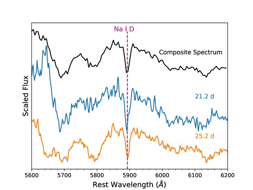
Figure 1: The narrow Na I D absorption dip due to the host galaxy, M61, in the two highest-SNR spectra (21.2 and 25.2 d) and the composite spectrum of SN 2020jfo.

3 Observations and Data Reduction

3.1 Photometric observations

3.1.1 Swift/UVOT photometry

Photometry of SN 2020jfo was obtained with the Neil Gehrels Swift Observatory (hereafter Swift) between 2020-05-07 and 2021-01-30 at 26 epochs. The transient was bright in all near-UV (NUV) and optical filters of the Swift/UVOT instrument. The UVOT data were reduced using the standard pipeline available in the HEAsoft software package. Observations at each epoch were conducted using one or several orbits. To improve the SNR in a given band at a particular epoch, we coadded all orbit data for that corresponding epoch using the HEAsoft routine uvotimsum. We used the routine uvotdetect to determine the correct position of the transient (which is consistent with the ground-based optical observations) and the routine uvotsource to measure the apparent magnitude of the transient by performing aperture photometry. For source extraction we used a small aperture of radius 3$\aas@@fstack{\prime\prime}$5, while an aperture of radius $100^{\prime\prime}$ was used to determine the background. There is a possibility that when multiple photons are coincident on the same area of the UVOT detector, it does not count all the photons, an effect known as “coincidence loss." The uvotsource routine makes the necessary correction to compensate for the coincidence loss. All of the UVOT photometry presented here is corrected for coincidence loss.

The field was also visited by Swift in the year 2008, to follow the Type II SN 2008in (Roy et al., 2011b), which exploded at the outskirt of another arm of the host. We have used those previous UVOT frames to calculate the host contribution at the location of SN 2020jfo. The host magnitudes at the transient location are $19.38\pm 0.07$, $19.34\pm 0.08$, $19.02\pm 0.05$, $18.49\pm 0.04$, $17.61\pm 0.07$, and $17.34\pm 0.09$ mag in the UVOT $uw2$, $um2$, $uw1$, $uvu$, $uvb$, and $uvv$ bands, respectively. To obtain the host-subtracted magnitudes of SN 2020jfo, we first subtracted the coincidence-loss-corrected count rate of the galaxy computed from the pre-SN observations, from the coincidence-loss-corrected count rate of SN 2020jfo calculated from the images where the SN exists. Then the host-subtracted count rates of the SN were converted to AB magnitudes (Oke & Gunn, 1983). The uncertainties in the final photometry were obtained by propagating the error associated with the host magnitude and the error in the “unsubtracted magnitudes" in quadrature. Our photometry in AB mag is listed in Table 6.

3.1.2 Optical photometry

Photometric follow-up observations of SN 2020jfo were carried out with telescopes in the Las Cumbres Observatory (LCO) under the Global Supernova Project (GSP) in $BVg^{\prime}r^{\prime}i^{\prime}$ filters between 2020-05-07 to 2021-07-13 at 53 epochs. Data between 2020-05-07 to 2021-02-22 at 44 epochs in the clear and $BVRI$ filters were also taken with the 1.04 m Sampurnanand Telescope (ST), the 1.3 m Devasthal Fast Optical Telescope (DFOT), and the 3.6 m Devasthal Optical Telescope (DOT) located in ARIES, Nainital, India, as well as with the 0.76 m Katzman Automatic Imaging Telescope (KAIT; Filippenko et al. 2001) and the 1.0 m Nickel telescope at Lick Observatory. The earliest $r$-band photometric point was taken with the 10.4 m GTC. The instrument details of the respective telescopes are given in Table 7. Preprocessing of the data, including bias and flat correction, was done using Python modules. The Cosmicray task in IRAF was used for the removal of cosmic rays. Multiple frames observed on the same night were median-combined in order to increase the SNR. We performed image subtraction on the cleaned observed frames to compute the true flux of the transient. For the ST and DFOT observations, we used an IRAF and DAOPHOT II (Stetson, 1987) based routine developed by Roy et al. (2011a), with the template taken on 2011-01-04 (see Roy et al. 2011b). The instrumental magnitudes of the SN were estimated using DAOPHOT II.

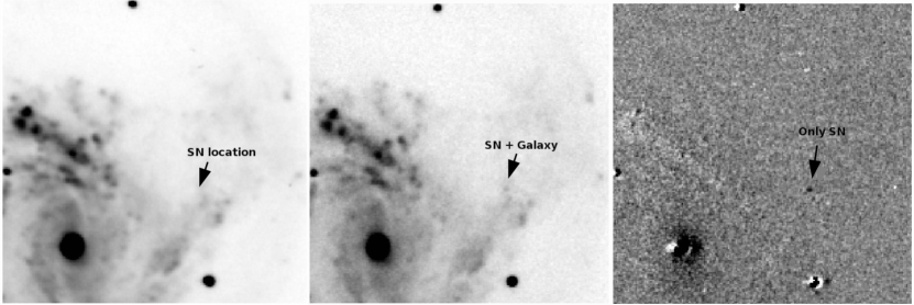
Figure 20: Measurement procedure of the true SN flux. The left and middle cutouts respectively present the template and transient frames, marking the SN locations observed from ST in the $V$ band. The template (left panel) frame was acquired on 2011-01-04 (see Roy et al. 2011b), whereas the middle panel represents the observation done on 2021-01-07. Both cutouts cover the same region of the sky, each of dimension $\sim 2.5\arcmin\times 2.5\arcmin$, and the location of the SN has been marked. In both cutouts north is up and east is to the left. The right panel shows the subtracted frame, where the SN has been marked. We performed the template subtraction on the ST and DFOT frames using the routine outlined by Roy et al. (2011a). The point-spread-function (PSF) photometry was done on each of the subtracted frames. The results obtained from this routine are consistent with the photometry obtained from HOTPANTS.

The LCO GSP data were reduced with the lcogtsnpipe pipeline (see Valenti et al. 2016a). For the LCO data, image subtraction was carried out using High Order Transform of PSF ANd Template Subtraction (HOTPANTS). We used the images obtained on 2021-07-17, when the SN faded below the detection threshold of the 1 m LCO telescopes, as the template. The instrumental SN magnitudes were calibrated using the magnitudes of a number of local standard stars in the SN field obtained from the AAVSO Photometric All-Sky Survey (APASS) catalogue, whereas the ST and DFOT photometric data were calibrated using the magnitudes of the field standards marked by Roy et al. (2011b). The data from KAIT and the 1.0 m Nickel telescope were reduced using a custom pipeline detailed by Stahl et al. (2019). An image-subtraction procedure was also applied in order to remove the host-galaxy light. The Pan-STARRS1 catalog was used for calibration. Apparent magnitudes were all measured in the KAIT4/Nickel2 natural system, then transformed back to the standard system using local calibrators and colour terms for KAIT4 and Nickel2 (Stahl et al., 2019). Figure 20 shows the template-subtracted image of SN 2020jfo. The calibrated SN magnitudes are listed in Tables 8, 9, and 10.

3.2 Optical and near-infrared spectroscopy

Spectroscopic observations of SN 2020jfo were conducted at 26 epochs between 2020-05-06 and 2021-05-04 using the 2.0 m Faulkes Telescope North (FTN) and Faulkes Telescope South (FTS) of the LCO Network (again via the Global Supernova Project), the 3.0 m Shane telescope at Lick Observatory, the 3.6 m DOT (ADFOSC; Omar et al. 2019), and the 10.4 m GTC. The details of the instruments used are given in Table 7. The one-dimensional (1D) wavelength- and flux-calibrated spectra were extracted using the floydsspec pipeline (Valenti et al., 2014) for the LCO data. Spectroscopic reduction of the Shane, DOT, and GTC data were done using standard tasks in IRAF which include preprocessing, extraction of the 1D spectrum, wavelength calibration, and flux calibration. The slit-loss corrections were accounted for by scaling the spectra to the photometry at the same or nearby epoch. We also corrected the spectra for the heliocentric redshift of the host galaxy. The log of spectroscopic observations is presented in Table 11.

Near-infrared (NIR) spectra of SN 2020jfo were obtained with the SpeX (Rayner et al., 2003) spectrograph installed on the 3.0 m NASA Infrared Telescope Facility (IRTF) at three epochs (2020-05-13, 2020-05-24, and 2020-06-15). The spectra were taken in both the PRISM and SXD mode with a slit size of $0\aas@@fstack{\prime\prime}5\times 15^{\prime\prime}$. The spectra were taken using the classic ABBA technique, and were reduced utilising the Spextool software package (Cushing et al., 2004). The telluric absorption corrections were done using the XTELLCOR software. The log of NIR spectroscopic observations is given in Table 11.

4 Light curves of SN 2020jfo

4.1 Light-curve rise and explosion epoch

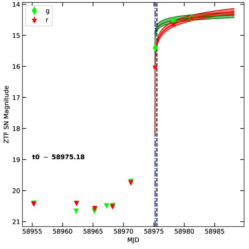
Figure 2: The ZTF-public $g$-band and $r$-band data of the rising phase of SN 2020jfo. The downward arrows show the upper limits. The black dashed vertical line marks the epoch (MJD 58975.5) of the first spectrum reported on the TNS. The blue dot-dashed vertical line marks the date of discovery (MJD 58975.203), whereas the date of explosion ($t_{0}$) obtained through power-law fitting is MJD 58975.18.

We used the ZTF-public data to compute the rise time of the transient. The object was first detected before its peak in the ZTF $r$ band on MJD 58975.203, considered the epoch of discovery in this paper. A third-order polynomial fit to the early part of the ZTF $r$ and $g$ light curves shows that the transient attained its peak at MJD $58981.698\pm 1.514$ in the observer’s frame. Figure 2 represents the early-time ZTF photometry along with the pre-SN nondetection ($3\sigma$) limits. The limit in nondetection (difference between last nondetection and first detection) is roughly 3.9 days, which also indicates the early discovery of the SN. The epoch of spectral classification (MJD 58975.5) is marked by the black dashed vertical line, whereas the epoch of discovery is marked by the blue dot-dashed line. We have assumed that during the early rising phase, the transient’s flux ($f$) evolved with time ($t\geq t_{0}$) according to a power law, $f\propto(t-t_{0})^{\beta}$ ($f=0$ for $t\leq t_{0}$). Here $t_{0}$ is the epoch of explosion and $\beta$ is the temporal index. The typical upper limits of the ZTF photometry during early nondetections are respectively $20.49\pm 0.10$ mag and $20.47\pm 0.10$ mag in $g$ and $r$. We have further assumed that for $t<t_{0}$, the fluxes at the SN location correspond to these upper limits. The power-law fit to the rising part of the light curves gives $t_{0}\approx 58975.18$, consistent with the date of explosion computed by Sollerman et al. (2021) and Singh Teja et al. (2022).

A comparison of the classification spectrum taken with the Liverpool Telescope/SPRAT on 2020-05-06 (MJD 58975.92) with early-time spectra of Type II events using GELATO shows that SN 2020jfo was roughly 3.8 days old on 2020-05-06. This implies that the epoch of explosion according to the spectral classification is MJD 58972.12. Furthermore, we run the SED matching code SNID (Blondin & Tonry, 2007) to constrain the explosion epoch of SN 2020jfo. We perform the spectral fitting of the same classification spectrum obtained with the Liverpool Telescope/SPRAT. The “rlap" parameter quantifies the quality of the fit, with a higher value implying a better correlation. The best match, with rlap parameter 4.9, is found with the spectrum of SN 2013ej obtained 3.7 days after explosion. Based on this, we estimate the age of SN 2020jfo on 2020-05-06 to be 3.7 days since explosion, which translates to MJD 58972.20 as the date of explosion. Anderson et al. (2014) and Gutiérrez et al. (2017) have indicated that this method is consistent with the last-nondetection method with an uncertainty of $\pm 5$ days.

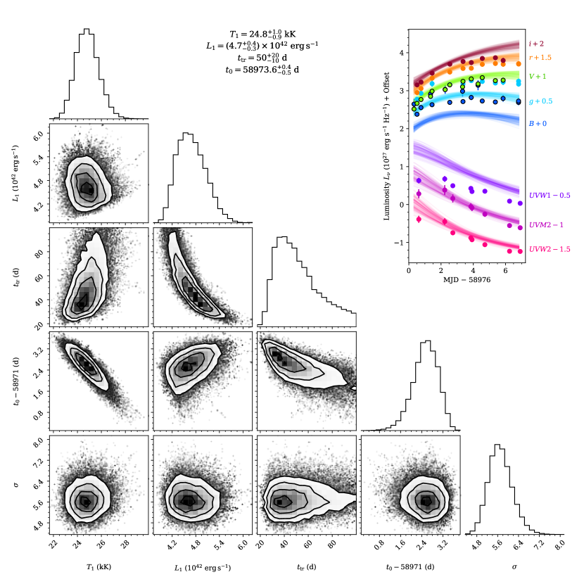
Figure 3: The fit to the Sapir & Waxman (2017) shock-cooling model using the method described by Hosseinzadeh et al. (2018). Posterior probability distributions and correlation between parameters of SN 2020jfo are shown in the corner plot. The parameters corresponding to the temperature and luminosity of the SN 1 day after the explosion ($T_{1}$, $L_{1}$), the time of explosion ($t_{0}$), and the time at which the envelope becomes transparent ($t_{\rm tr}$) are shown. The top-right panel displays 100 fits randomly drawn from the MCMC routine (Hosseinzadeh & Gomez, 2020) to fit the early-time photometry. The $\sigma$ parameter depicts the intrinsic scatter of the model. The fit deviates largely from the observed light curves, and hence the estimated parameters from the fit are not used in the paper.

Additionally, we adopt early light-curve modeling, following the prescription of Sapir & Waxman (2017), to estimate the explosion epoch. The early-time emission from SNe is powered by shock cooling and provides useful insights on the radius and pre-explosion evolution of the progenitor. The Markov Chain Monte Carlo (MCMC) code developed by Hosseinzadeh & Gomez (2020) is used to obtain posterior probability distributions of temperature and luminosity of the SN 1 day after explosion ($T_{1}$, $L_{1}$), the time of explosion ($t_{0}$), and the time at which the envelope becomes transparent ($t_{\rm tr}$) simultaneously. We model the early-time light curve of SN 2020jfo using the multiband data up to MJD 58983.0 with $n=1.5$ for an RSG and uniform priors for all parameters. The model outputs the blackbody temperature and total luminosity as a function of time for each combination of the parameters, which are then translated to measured fluxes for each photometric point and all the light curves are simultaneously fitted. The parameter $\sigma$ is a measure of the intrinsic scatter of the model for which a log uniform prior is used. The posterior probability distributions and correlation between parameters of SN 2020jfo are shown in Figure 3. The model fits the V, r, and i bands reasonably well at least up to 58979 MJD. However, in the B, g, and UV bands, the model does not fit well; specifically, the B and g data are much redder and the UVW1 band data are bluer than the models allow. Also, the model has a large intrinsic scatter ($\sigma=5.7$). Thus, although the fit converges to an explosion epoch MJD $58973.6^{+0.4}_{-0.5}$ d, and the temperature and luminosity 1 day after explosion respectively converge to $T_{1}=24.8^{+1.0}_{-0.9}\times 10^{3}$ K and $L_{1}=4.7^{+0.4}_{-0.3}\times 10^{42}$ erg s^-1, we cannot accept these numbers as reliable estimates owing to the poor quality of the fits. The poor fitting of the model suggests that there is likely some circumstellar material (CSM) interaction which is powering the early-time light curve.

The explosion epoch from the different methods described above are 58975.0 (from the light curve rise), 58972.12 (from GELATO), and 58972.20 (from SNID). Here we use the mean MJD 58973.1 as the explosion epoch and the standard deviation of these estimates (1.6 day) as the uncertainty for further analysis, consistent with the explosion epochs MJD $58974.70^{+0.5}_{-3.5}$ and $58973.8^{+0.49}_{-0.46}$ used by Sollerman et al. (2021) and Singh Teja et al. (2022), respectively.

4.2 Light-curve evolution of SN 2020jfo

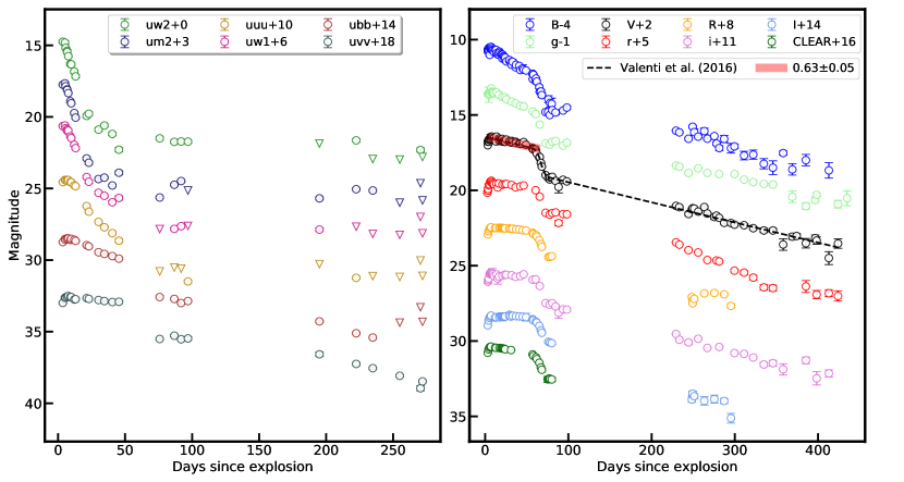
Figure 4: The Swift UVOT and optical light curves of SN 2020jfo since the date of explosion. The inverted triangles represent upper limits in the UVOT light curves. The light curves are offset by arbitrary numbers for display clarity. The dashed line represents the best fit to the $V$ band using Valenti et al. (2016b).

The Swift UVOT and multiband optical light curves of SN 2020jfo are shown in Figure 4. The optical light curves of SN 2020jfo initially rise to a peak in the BVg’r’i’ bands. We estimate the peak magnitudes and the corresponding epoch at maximum brightness in the BVg’r’i’ bands by fitting a parabolic function to the early-time data points ($t\leq 16$ day). The uncertainty in the maximum epoch is obtained by adding in quadrature the fitting error and the uncertainty in the explosion epoch. The values are listed in Table 2. During the plateau phase, the SN declines with a rate of $2.12\pm 0.06$, $0.70\pm 0.07$, and $0.30\pm 0.08$ mag (50 day)^-1 in B, V, and r, respectively. As the SN evolves, the light curve falls from maximum and settles onto a plateau phase. The end of the plateau phase is marked by a sharp drop in magnitude, followed by an exponentially decaying phase powered by the radioactive decay of ⁵⁶Co to ⁵⁶Fe. The slope of the radioactive tail in $V$ is $1.60\pm 0.07$ mag (100 d)^-1, which is steeper than the ⁵⁶Co to ⁵⁶Fe decay rate (0.98 mag (100 d)^-1), indicating partial trapping of $\gamma$-rays in the ejecta.

Table 2: Peak magnitudes and phase of peak time in BVg’r’i’ bands

Band	Epoch at maximuma	Peak magnitude
	( days)	(mag)
B	7.8$\pm$1.6	14.634$\pm$0.004
g’	8.1$\pm$1.6	14.484$\pm$0.001
V	10.5$\pm$1.8	14.512$\pm$0.014
r’	10.2$\pm$1.6	14.460$\pm$0.008
i’	10.8$\pm$1.6	14.514$\pm$0.008

^aPhase with respect to the explosion epoch (MJD 58973.1).

We fit the V-band light curve using the expression given by Valenti et al. (2016b),

$y(t)=\frac{-a_{0}}{1\,+\,{\rm exp}{(t-t_{\rm pt})/w_{0}}}+p_{0}\,t+m_{0}$ .

This is used to estimate the drop in magnitude from plateau to the tail phase, $a_{0}$, the duration of the transition phase ($\sim 6\times w_{0}$), $t_{\rm pt}$, and a transition point between the end of the plateau (and the onset of the radioactive tail) and the decline rate of the radioactive tail phase, $p_{0}$. The estimated value of $t_{\rm pt}$ of SN 2020jfo is $67.0\pm 0.6$ days, which is similar to that of SN 2006Y ($66.8\pm 4$ days) but shorter than that of the other SNe II in the comparison sample. Singh Teja et al. (2022) estimated a plateau length of $58\pm 2$ days, which corresponds to the parameter OPTd from Anderson et al. (2014), whereas we estimated $t_{\rm pt}$, which is roughly equivalent to OPTd + 0.5 times the duration of the transition phase. Considering this, our estimated $t_{pt}$ value is consistent with Singh Teja et al. (2022) within the uncertainties. The best-fitting value of $a_{0}$ is $1.68\pm 0.09$ mag, which lies in the range of Type II SNe (1–2.6 mag) as suggested by Valenti et al. (2016b). SN II 2006Y has also been reported to have a similar drop in magnitude ($1.75^{+0.23}_{-0.15}$) during the transition phase. However, the duration of the transition phase ($6\times w_{0}$) of SN 2020jfo (13.3 days) is shorter than that of SN II 2006Y (25.7 days). This could be due to different amounts of Ni mixing (Goldberg et al., 2019). The values of best-fit parameters are listed in Table 3 and the best fit in the $V$ band is shown in Figure 4 by the dashed line.

Table 3: The best-fitted s_50V slope of V-band lightcurve of SN 2020jfo between start and end phase. The measurement of slope is given in magnitudes per 50 days. The best fitted V-band light curve parameters using Valenti et al. (2016b) model are also given here.

Slope	Decline Rate	Start Phase	End Phase
s50V	0.63$\pm$0.05	8.8	60.7
tpt (d)	a0 (mag)	w0 (d)	p0 (mag/d)
67.0 $\pm$ 0.6	1.68 $\pm$ 0.09	2.22 $\pm$ 0.68	0.0134 $\pm$ 0.0003

Table 4: Properties of the SNe in the comparison sample

Object	Host Galaxy	Distance	Total	Ejected	M${}_{V}^{peak}$	M${}_{V}^{50d}$	tpt	References
			Extinction	56Ni Mass
		(Mpc)	E(B-V) (mag)	($M_{\odot}$)	(mag)	(mag)	(days)
SN 1995ad	NGC2139	22.91$\pm$1.64	0.035	0.028	-17.64$\pm$0.29	-16.27$\pm$0.11	50†	6
SN 1999em	NGC 1637	11.7$\pm$0.1	0.10	0.042	-16.86$\pm$0.07	-16.71$\pm$0.06	118.1$\pm$1.0	1, 2, 3, 7
SN 2005cs	M 51	8.40	0.12	<0.003	-14.81$\pm$0.37	-14.55$\pm$0.32	126.0$\pm$0.5	4, 5, 7
SN 2006Y	anonymous	146.0	0.11	>0.050	-18.09$\pm$0.01	-16.75$\pm$0.02	66.8$\pm$4	7, 8
SN 2006ai	ESO 5-G9	67.5	0.11	>0.034	-18.23$\pm$0.02	-17.00$\pm$0.01	72.4$\pm$5	7, 8
SN 2007od	UGC12846	25.7$\pm$1.84	0.038	0.02	-18.00$\pm$0.16	-17.31$\pm$0.13	45†	9
SN 2015ba	IC 1029	34.8$\pm$0.7	0.46$\pm$0.05	0.032$\pm$0.006	-17.68$\pm$0.17	-17.05$\pm$0.15	140.7$\pm$0.2	10
SN 2016egz	anonymous	100.0	0.01	–	-18.46$\pm$0.03	-17.55$\pm$0.05	71.2‡ $\pm$ 0.5	8
SN 2020jfo	M61	14.51$\pm$1.38	0.17$\pm$0.09	0.03$\pm$0.01	-16.90$\pm$0.34	-16.69$\pm$0.44	67.0$\pm$0.6	This work

• ^† OPTd

• ^‡ t_pt estimated in this work

• (1) Hamuy et al. (2001b), (2) Leonard et al. (2002), (3) Leonard et al. (2003), (4) Pastorello et al. (2006), (5) Pastorello et al. (2009), (6) Inserra et al. (2013), (7) Valenti et al. (2016b), (8) Hiramatsu et al. (2021b), (9) Inserra et al. (2011), (10) Dastidar et al. (2018)

SN 2020jfo has good UVOT data coverage until late times, unlike most other SNe II, which have low apparent luminosity owing to host-galaxy extinction and large distances. The UVOT light curves decay rapidly until $\sim 23$ days since explosion with a rate of $0.28\pm 0.01$, $0.30\pm 0.01$, and $0.21\pm 0.01$ mag day^-1 in the uw2, um2, and uw1 bands respectively. We compare the UV absolute magnitudes in the UVOT filters of SN 2020jfo with those of some other well-observed Type II SNe in Figure 5. The sample is chosen based on the availability of good cadence light curves in UV bands. This sample comprises the following SNe: SN 2005cs (Pastorello et al. 2009; Brown et al. 2009), SN 2006bp (Dessart et al. 2008), SN 2012aw (Bose et al. 2013), SN 2013ab (Bose et al. 2015a), SN 2013by (Valenti et al. 2015), SN 2013ej (Bose et al. 2015b), SN 2014G (Bose et al. 2016), and SN 2016at (Bose et al. 2019). All Type II SNe show a rapid decline in the first 20 days of evolution in the UV filters. SN 2020jfo falls on the fainter end of the normal-luminosity SNe II and is brighter than the low-luminosity SN 2005cs. Some of the comparison SNe with good data coverage, such as SNe 2013by and 2013ab, show a constant-luminosity phase in the UV bands corresponding to the plateau phase in optical bands. However, the UV light curves of SN 2020jfo do not exhibit any plateau phase.

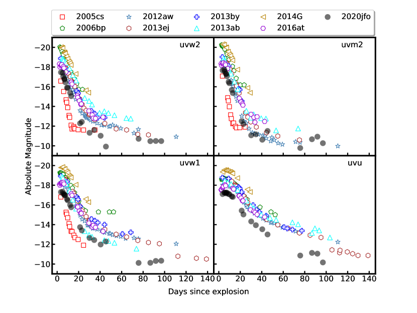
Figure 5: The comparison of Swift UVOT absolute magnitude light curves of SN 2020jfo with those of some well-observed Type IIP SNe observed with Swift.

To examine the behaviour of SN 2020jfo in the optical bands, we assemble a comparison sample of SNe with varying plateau lengths and a range of explosion properties: SNe 1995ad (short plateau; Inserra et al. 2012), 1999em (normal Type IIP; Elmhamdi et al. 2003), 2005cs (low-luminosity Type IIP; Pastorello et al. 2006, Pastorello et al. 2009), 2006Y (short plateau; Hiramatsu et al. 2021b), 2006ai (short plateau; Hiramatsu et al. 2021b), 2007od (short plateau; Inserra et al. 2011), 2015ba (long plateau Type IIP; Dastidar et al. 2018), and 2016egz (short plateau; Hiramatsu et al. 2021b). The parameters of the comparison sample are listed in Table 4.

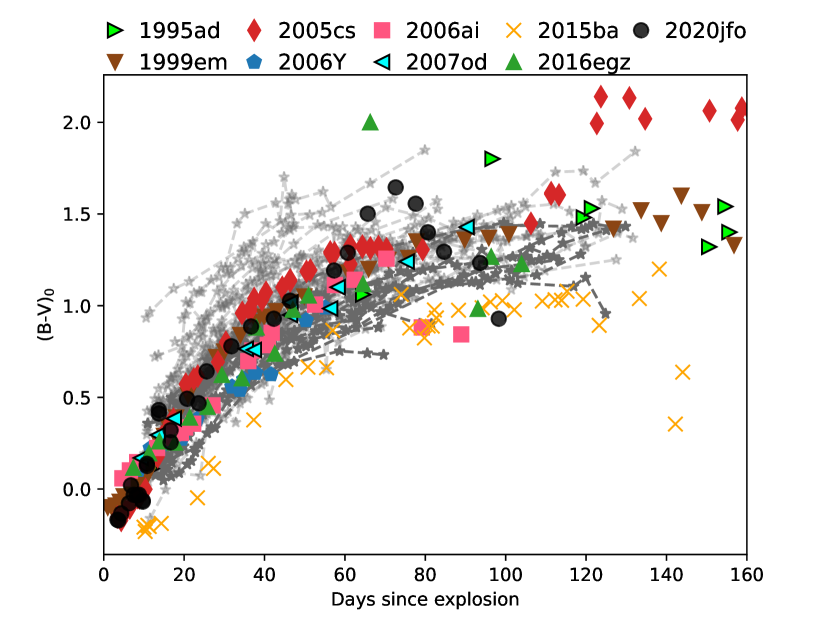
Figure 6: $(B-V)_{0}$ colour evolution of SN 2020jfo compared with the SN II sample used in this paper.

The colour evolution provides information about the dynamics of the SN ejecta. The temporal evolution of the reddening-corrected $(B-V)_{0}$ colour of SN 2020jfo is depicted in Figure 6 along with that of the comparison sample of SNe and the sample of Type II SNe from de Jaeger et al. (2018) (shown in grey) and a subset of this sample with negligible host extinction (shown with grey stars). All SNe exhibit roughly the same trend in $(B-V)_{0}$ colour — a gradual transition to redder colours in the first 50 days, followed by a flattening until the end of the plateau phase. Owing to expansion of the ejecta, the $(B-V)_{0}$ colour of SN 2020jfo becomes redder by 1.2 mag until the end of the plateau phase. Thereafter, SN 2020jfo starts transitioning from the plateau to the tail phase at $\sim 70$ days, which is marked by a steeper rise to redder colours. As the SN settles in the exponentially decaying tail phase, the $(B-V)_{0}$ colour gradually becomes bluer by 0.7 mag. SN 2020jfo and the other SNe II with shorter plateau lengths (SNe 1995ad, 2006Y, 2006ai, 2007od, and 2016egz) do not show the constant-colour phase corresponding to the plateau phase as seen in other SNe II such as SNe 1999em, 2005cs, and 2015ba; almost immediately after 50 days, the light curve transitions from the plateau to the tail phase in Type II SNe with shorter plateau. Like SN 2020jfo, a sudden transition to redder colours at the end of the plateau phase is also evident in SN 2005cs; however, the latter does not display a transition to bluer colours in the nebular phase. SN 2006ai also exhibits this transition to bluer colours in the nebular phase.

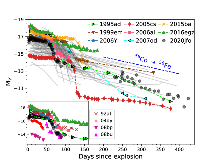
Figure 7: Absolute $V$-band light curve of SN 2020jfo compared with the Type II SNe in the comparison sample. The grey lines represent the light curves of 116 SNe II having different plateau lengths from Anderson et al. (2014). The inset shows the comparison of SN 2020jfo with other Type II SNe having similar plateau lengths in the comparison sample used in the paper and the sample of Anderson et al. (2014).

The absolute magnitude $V$-band light curve of SN 2020jfo is shown along with the comparison sample in Figure 7. In terms of brightness, SN 2020jfo has similar absolute magnitudes in the early and plateau phase as the prototypical Type IIP SN 1999em, with a remarkably early drop from the plateau as compared to SN 1999em. The plateau length of SN 2020jfo is rather similar to that of the Type II SNe 1995ad, 2006Y, and 2006ai with plateau duration in the range 50–70 days. The peak of SN 2020jfo is $-16.90\pm 0.34$ mag, consistent within uncertainties with that obtained by Singh Teja et al. (2022). The Type II SNe having shorter plateau duration (SNe 1995ad, 2006Y, 2006ai, 2007od, and 2016egz) are brighter than SN 2020jfo by at least 0.7 mag at peak and have a steeper post-peak decline rate (up to 20 days) than SN 2020jfo (2.5 mag (50 day)^-1, SN 1995ad; 3.0 mag (50 day)^-1, SN 2006Y; 1.7 mag (50 day)^-1, SN 2006ai; 1.2 mag (50 day)^-1, SN 2007od; 2.2 mag (50 day)^-1, SN 2016egz). SN 2020jfo is brighter than the low-luminosity Type II SN 2005cs by $\sim 2$ mag in the plateau phase and fainter than the long-plateau SN 2015ba by 0.5 mag. The grey lines represent the light curves of 116 Type II SNe having different plateau lengths from Anderson et al. (2014). The sample of Anderson et al. (2014) also consists of a few SNe II with relatively shorter plateaus (SNe 1992af, 2004dy, 2008bp, and 2008bu), which we have shown separately in the inset plot along with SNe 2020jfo, 1995ad, 2006Y, 2006ai, and 2016egz. Except for SNe 1992af, the other SNe II (SNe 1995ad, 2004dy, 2008bp, and 2008bu) have absolute magnitudes during the plateau phase similar to or lower than that of SN 2020jfo. As noted by Hiramatsu et al. (2021b), SN 1992af has an uncertain explosion epoch and hence might have a longer plateau duration. The tail-phase luminosity of SN 2020jfo is similar to that of SN 1999em and lower than that of the rest of the SNe in the comparison sample except for SN 2005cs. SN 2016egz has the highest tail luminosity, whereas SNe 2006Y and 2006ai have tail luminosities similar to that of SN 1999em. The inset plot shows that the Type II SNe with similar plateau magnitudes also have comparaable tail luminosities.

The ⁵⁶Ni mass is estimated from the tail bolometric luminosity following Hamuy (2003) using the tail $V$-band magnitudes. The tail luminosity ($L_{t}$) obtained from the $V$ magnitudes using the bolometric correction factor given by Hamuy (2003) at two epochs (72.2 and 80.2 days) are $2.19\pm 0.71\times 10^{41}$ erg s^-1 and $2.04\pm 0.66\times 10^{41}$ erg s^-1, respectively, which corresponds to a mean ⁵⁶Ni mass of $0.03\pm 0.01$ M_⊙. This is consistent with the ⁵⁶Ni mass obtained for SN 2020jfo by Sollerman et al. (2021) and Singh Teja et al. (2022).

5 Spectral Analysis

5.1 Spectroscopic evolution

Figure 8: The spectral evolution of SN 2020jfo from 2.8 days to 365.2 days since explosion with the prominent spectral features marked. Each spectrum is normalised with the median flux.

The spectral evolution of SN 2020jfo from 2.8 to 365.2 days since explosion is shown in Figure 8. At the early phase of the evolution (2.8–4.5 days), broad P Cygni profiles of H Balmer lines can be seen superimposed on a blue continuum. The spectra from 8.3 days reflect the transition from a hot to a cool SN envelope, as the photosphere begins to penetrate deeper into the metal-rich ejecta. These spectra mark the emergence of other lines from heavier atomic species such as Ca, Fe, Sc, Ba, Ti, and Na. Among these, the Fe II $\lambda\lambda$4950, 5169 lines appear from 18.9 days. Sc II lines, O I, and the Ca II NIR triplet gain prominence from day 40.2 and get stronger over time. By the end of the plateau phase, all weak and blended lines have evolved and become conspicuous. A high-velocity absorption dip blueward of the H$\alpha$ absorption minimum becomes apparent in the day 63–85 spectra.

For robust line identifications, we used SYNAPPS (Thomas, 2013) to reproduce the early-time (3.5 d) and photospheric-phase (32.4 d) spectra of SN 2020jfo (Figure 9). For modelling the early spectrum, we used H I and Ca II species. The photospheric velocity and blackbody temperature at 3.5 d as constrained from the modelling are 13,360 km s^-1 and 11,650 K, respectively. The photospheric spectrum is reproduced using H I, Ca II, Fe II, Na I, Ba II, Sc II, and Ti II lines. The Ti II, Sc II, and Ba II species mainly contribute in reproducing the 5200–6000 Å region. The photospheric velocity and blackbody temperature at 32.4 d as constrained from the modelling are 5476 km s^-1 and 8380 K, respectively. In both cases, the “detach" parameter has been deactivated, which means that the minimum ejecta velocity of all the ions will be the same as the photospheric velocity.

The day 63.3 spectrum marks the onset of the transition from the plateau to the nebular phase. All subsequent spectra up to day 85.1 are representative of the early nebular phase, when the outer ejecta have become optically thin. In the late nebular phase spectra (253.9–365.2 day), in addition to the H$\alpha$ emission, a number of forbidden emission lines such as [O I] $\lambda\lambda$6300, 6364 and [Ca II] can be seen. Also, the nebular spectra of SN 2020jfo show strong [Ni II] and [Fe II] forbidden emission which can be used as a diagnostic of the Ni-to-Fe mass ratio in the entire ejecta (Jerkstrand et al., 2015).

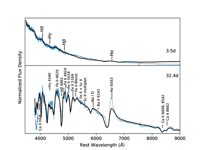
Figure 9: SYNAPPS modelling of the early (3.5 day) and plateau phase (32.4 day) spectra of SN 2020jfo (shown in black) marked with the lines identified from the spectral modelling.

The three NIR spectra of SN 2020jfo obtained on days 8.3, 19.3, and 41.2 are shown in Figure 10. The day 8.3 spectrum exhibits weak lines of Pa$\alpha$, Pa$\beta$, Pa$\gamma$, and He I, and a relatively strong Ca  II NIR triplet. The feature around $\lambda$10,800 in the day 8.3, 19.3, and 41.2 spectra is probably a He I and Pa$\gamma$ blend, although there is a possibility of C I formation at 10,691 Å. We used SYNAPPS to model the wavelength range 8000–13,500 Å in the day 19.3 spectrum using H I, He I, C I, and Ca II ions, and can reproduce this region well as shown in Figure 10. The presence of the C I line has been indicated in a few SNe II, such as SNe1999em (Hamuy et al., 2001a), 2005cs (Pastorello et al., 2009), and 2012aw (Davis et al., 2019). We compare the NIR spectra of SN 2020jfo with those of other SNe II like SNe 1999em (Hamuy et al., 2001a), 2005cs (Pastorello et al., 2009), 2012aw (Dall’Ora et al., 2014), and 2012ec (Barbarino et al., 2015) at nearby epochs in Figure 10. Overall, the NIR spectra of SN 2020jfo show similarity with other SNe II. The day 8.3 spectrum of SN 2020jfo is similar to the day 5.7 spectrum of SN 1999em and the day 7.0 spectrum of SN 2012ec, all showing the classical feature at 10,830 Å, while the day 8.0 spectrum of SN 2012aw does not exhibit any conspicuous line at this wavelength. The 10,549 Å absorption feature in the day 21.7 spectrum of SN 1999em was suggested to be possibly a blend of C I $\lambda$10,691 and He I $\lambda$10,830 (Hamuy et al., 2001a). However, in the day 62.0 spectrum of SN 2005cs, this feature was suggested to be mostly due to P$\gamma$, Sr II $\lambda$10,915, and C I $\lambda$10,691, with less dominance of He I $\lambda$ 10,830 than in other CCSNe (Pastorello et al., 2009). In SN 2020jfo, this feature is mostly dominated by Pa$\gamma$, He I, and C I. There is possibly no formation of Sr II at least until day 19.3 in SN 2020jfo; introducing the ion deteriorated the SYNAPPS fit.

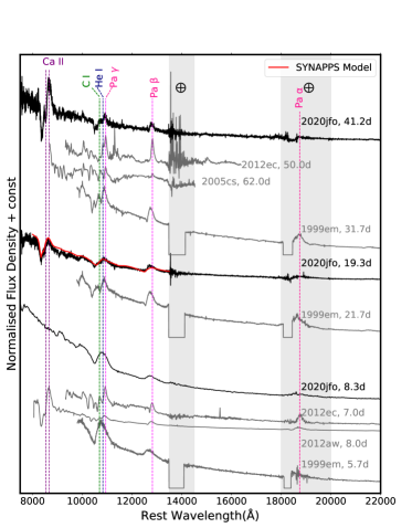
Figure 10: The NIR spectral evolution of SN 2020jfo compared with that of other Type II SNe. The SYNAPPS model of the day 19.3 spectrum in the wavelength range 8000–13,500 Å using H I, He I, C I, and Ca II species is shown in red.

5.2 Comparison with other SNe

We compare the spectra of SN 2020jfo at early times ($\sim 8.3$ day), the plateau ($\sim 40.2$ day), and the nebular phase ($\sim 365.2$ day) with the spectra of the comparison sample at similar epochs. The spectroscopic comparison sample is composed of the same SNe II that are defined in Section 4.2 and listed in Table 4.

At the early phase ($\sim 8$ day), Figure 11 indicates that the spectrum of SN 2020jfo displays broad H Balmer emission on a blue continuum similar to SNe 1995ad, 1999em, and 2007od. The comparable-epoch spectra of Type II SNe 2006Y (12.7 day), 2016egz (6.8 day), and SN 2015ba (7.8 day) are mostly blue and featureless corresponding to the shock-cooling phase. In contrast, the day 8 spectrum of SN 2005cs shows well-developed P Cygni profiles of H Balmer lines, Ca II H&K, and feebly visible Fe II, suggesting cooler photospheric temperatures for SN 2005cs.

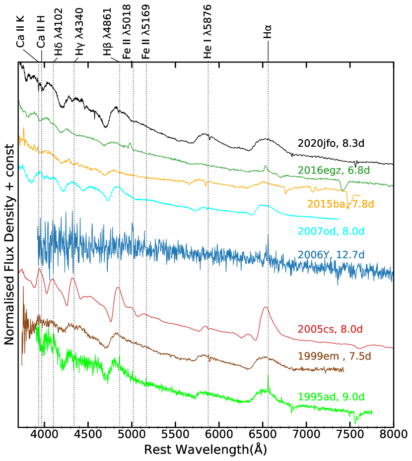
Figure 11: The spectrum of SN 2020jfo at $\sim 8$ day is compared with early-time spectra of other SNe II in the comparison sample.

In Figure 12, we compare the plateau-phase spectrum ($\sim 40.2$ day) of SN 2020jfo with those of the comparison sample. The plateau-phase spectrum of SN 2020jfo is likewise similar to that of SNe 1995ad, 1999em, 2007od, and 2015ba. Unlike the other Type II SNe 2006Y and 2016egz, the spectrum of SN 2020jfo exhibits a substantial absorption component of the P Cygni profile of H$\alpha$, which is shown by zooming in on the wavelength region 6000–6800 Å. The plateau spectrum of SN 2020jfo also shows well-developed Fe II and feebly visible Sc II and Ba II lines. The Na I D absorption is prominent in SN 2020jfo, similar to some Type II SNe with short plateau duration such as SNe 1995ad and 2006ai, but unlike the other short-plateau Type II SNe 2006Y, 2007od, and 2016egz. The Ca II NIR triplet is also prominent in SN 2020jfo, similar to SNe 1995ad, 1999em, 2005cs, and 2015ba, and can be seen developing in the spectra of SNe 2006Y, 2006ai, and 2016egz.

Figure 12: The plateau-phase spectrum of SN 2020jfo at $\sim 40$ day is compared with those of other SNe in the comparison sample. The wavelength region 6000–6800 Å is zoomed in and plotted in velocity space with respect to H$\alpha$, which highlights the similarity of the absorption component of H$\alpha$ in SN 2020jfo with the prototypical Type II SN 1999em.

In Figure 13, we compare the nebular ($\sim 365.2$ day) spectrum of SN 2020jfo with that of other SNe in the comparison sample at similar phases. Only one short-plateau SN 2016egz has a nebular spectrum after 300 days, which is mostly featureless. This is most likely due to host-galaxy contamination given its proximity to the host, as is also suggested by the the prominent narrow [O III] $\lambda\lambda$4959, 5007 emission lines. The H$\alpha$ feature is pronounced in emission in all of the comparison spectra. The [O I] $\lambda\lambda$6300, 6364 doublet and [Ca II] $\lambda\lambda$7292, 7324 are very prominent in SN 2020jfo, similar to the other Type II SNe 1999em, 2005cs, and 2015ba. The nebular spectrum of SN 2020jfo exhibits strong [Ni II] $\lambda$7378 emission which is indiscernible in the comparison sample. Overall, the features in the SN 2020jfo nebular spectrum are more similar to the spectra of SNe 1999em, 2005cs, and 2015ba, except the inconspicuous Ca II NIR triplet in the spectrum of SN 2020jfo (unlike these other SNe).

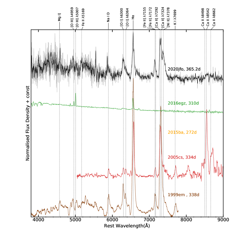
Figure 13: The nebular-phase spectrum of SN 2020jfo at $\sim 365$ day is compared with other SNe in the comparison sample. The nebular features in SN 2020jfo are similar to those seen in SN 1999em.

Thus, despite a short plateau duration, the spectral features of SN 2020jfo are more similar to those of normal Type II SNe. The length of the plateau phase is determined by the mass of the H envelope as well as the time it takes for the H to recombine. The progenitor of SN 2020jfo is likely to have an H envelope mass comparable to that of a typical SN II, but with a shorter recombination time. However, rapidly expanding ejecta could explain the shorter recombination time; except for the first two epochs, the ejecta velocity of SN 2020jfo follows the mean velocity curve of normal Type II SNe (see Figure 14). The plateau duration, however, is also affected by the extent of ⁵⁶Ni mixing in the ejecta, with a higher degree of mixing resulting in shorter plateaus (Pumo & Zampieri, 2013; Goldberg et al., 2019).

5.3 Velocity evolution

The expansion velocity of the ejecta can be estimated from the minima of the absorption component of the P Cygni profile of various lines. We estimate the line velocities of a few prominent features in SN 2020jfo and show their evolution with time in Figure 14 (top panel). The H$\alpha$ and H$\beta$ velocities are comparable at early phases (10,200 km s^-1 and 9900 km s^-1 at day 8) and greater than the velocity of other metal lines. As time proceeds, the H$\alpha$ velocity is higher than all other line velocities, showing it to be part of the outer expanding layer of ejecta. The velocity of the Fe II line gives a fair estimate of the expansion velocity of the photosphere, and it is estimated to be around 8400 km s^-1 at $\sim 15$ days; it decays down to 1600 km s^-1 at the onset of the nebular phase. The decreasing trend of velocity shows that as time proceeds we are looking at the inner, lower-velocity layers of the ejecta owing to a decrease in the opacity resulting from the expansion of the ejecta.

The line velocities of SN 2020jfo are compared with those of other SNe in the sample. Figure 14 (bottom three panels) show the evolution of H$\alpha$, H$\beta$, and Fe II line velocities. The mean velocity evolution and the standard deviation for a sample of 122 Type II SNe from Gutiérrez et al. (2017) is shown with a blue solid line and grey shaded region, respectively. Overall, the velocities of SN 2020jfo are lower than the velocities of the SNe in the comparison sample except SN 2005cs, and lie toward the edge of the grey band. The velocities of other SNe II having shorter plateaus are typically higher than that of SN 2020jfo. The Fe II velocity of SN 2020jfo at day 15 after explosion is $\sim 1900$ km s^-1 higher than the mean velocity.

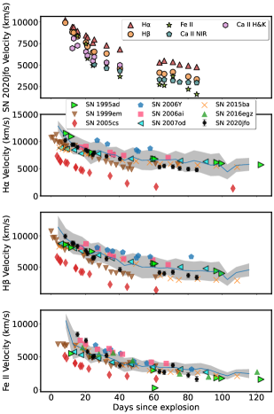
Figure 14: The evolution of line velocities of a few prominent lines in SN 2020jfo is shown in the top panel. The bottom three panels display a comparison of the velocity evolution of H$\alpha$, H$\beta$, and Fe II lines of SN 2020jfo and the comparison sample. The mean velocities and the standard deviations of the velocities in the SN II sample from Gutiérrez et al. (2017) are shown with a blue solid line and a grey band, respectively.

6 Progenitor and explosion properties

In this section, we adopt different techniques to estimate the progenitor properties, and we provide a cohesive picture of this analysis in Section 8.

6.1 Estimations from the nebular spectrum

The observed strengths of nebular lines, especially the [O I] $\lambda\lambda$6300, 6364 doublet, can serve as a diagnostic of the progenitor mass, as the nucleosynthetic yield depends strongly on the mass of the progenitor (Woosley & Weaver, 1995). Jerkstrand et al. (2014) generated models of nebular spectra for 12, 15, 19, and 25 M_⊙ progenitors for 0.062 M_⊙ of ⁵⁶Ni, assuming a distance of 5.5 Mpc. We compare the day 365.2 spectrum of SN 2020jfo to these models to get a handle on the mass of the progenitor as shown in Figure 15. As the SN is powered by the radioactive decay energy in the nebular phase, we scaled the day 400 model spectrum flux with the ratio of the ⁵⁶Ni mass of SN 2020jfo (0.030 M_⊙) to the ⁵⁶Ni mass of the model spectrum (0.062 M_⊙). Then the day 400 model flux was rescaled to the distance and phase (365.2 day) of the nebular spectrum of SN 2020jfo. We also used a scaling factor of 0.5, similar to Sollerman et al. (2021), owing to the partial trapping of $\gamma$-rays in SN 2020jfo. Before the comparison, we deredshifted the SN spectrum, scaled the spectrum to match the photometric flux so that the slit losses are taken care of, and applied reddening corrections. The SN spectrum best matches with the 12 M_⊙ model. However, the H$\alpha$ flux in the spectrum of SN 2020jfo is a factor of 3 lower than the model flux. The model also shows a prominent Ca II NIR triplet feature which is absent in the SN 2020jfo spectrum. The [O I] flux in the SN 2020jfo spectrum is comparable to the model spectrum, suggesting a progenitor ZAMS mass of $\sim 12$ M_⊙ for SN 2020jfo. We note here that Sollerman et al. (2021) and Singh Teja et al. (2022) also carried out this comparison with the nebular spectra of SN 2020jfo and our result is consistent with theirs.

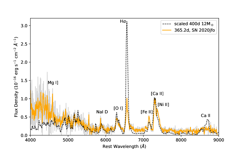
Figure 15: Comparison of the day 365.2 spectrum of SN 2020jfo with that of the scaled model spectra from (Jerkstrand et al., 2014).

The relative abundances of the different elements have been suggested to vary substantially with the helium core mass (Fransson & Chevalier, 1989); specifically, the [O I]/[Ca II] ratio has been used to estimate the progenitor’s ZAMS mass by several authors (e.g., Fransson & Chevalier 1989; Elmhamdi et al. 2004; Kuncarayakti et al. 2015). We estimated the [O I] and [Ca II] luminosity in the nebular spectrum (365.2 day) of SN 2020jfo to be $(1.13\pm 0.19)\times 10^{38}$ erg s^-1 and $(1.96\pm 0.06)\times 10^{38}$ erg s^-1, respectively, and the [O I]/[Ca II] ratio is $0.58\pm 0.10$. This ratio has been found to fall below 0.7 for Type II SNe, while for other CCSNe, the ratio is higher than 0.7 (Kuncarayakti et al., 2015). Thus, for SN 2020jfo, the [O I]/[Ca II] ratio coincides with the upper limit for SNe II. The fact that the ratio increases with increasing main-sequence mass suggests that the progenitor of SN 2020jfo falls on the upper end of the mass distribution for Type IIP SN progenitors.

6.2 Ni/Fe production ratio

Ni and Fe are essentially produced in the same region of the ejecta in Fe CCSNe, and the [Fe II] emission is stronger compared with [Ni II] in these events (Jerkstrand et al., 2012). Jerkstrand et al. (2015) presented an analytic method to determine the Ni/Fe ratio in nebular spectra of SNe in the 7100–7400 Å region, which we have applied here to SN 2020jfo. There are eight prominent emission lines in the 7100–7500 Å region: [Ca II] $\lambda\lambda$7291, 7323, [Fe II] $\lambda$7155, [Fe II] $\lambda$7172, [Fe II] $\lambda$7388, [Fe II] $\lambda$7453, [Ni II] $\lambda$7378, and [Ni II] $\lambda$7412. We fit this spectral region in the day 253.9, 255.9, and 365.2 spectra of SN 2020jfo using Gaussian components for these lines. Following the Jerkstrand model, we fixed the line ratios from the same species. Thus, the iron lines are constrained by $L_{7453}=0.31\,L_{7155}$, $L_{7172}=0.24\,L_{7155}$, and $L_{7388}=0.19\,L_{7155}$, and the nickel lines are constrained by $L_{7412}=0.31\,L_{7378}$. Furthermore, in this method, the full width at half-maximum (FWHM) velocity $v$ of all the emission lines are forced to be the same for a given epoch, so that there are four free parameters: $L_{7291,7323}$, $L_{7155}$, $L_{7378}$, and $v$.

In Figure 16, we show that a good fit in the day 365.2 spectrum is obtained for $L_{7291,7323}=(1.96\pm 0.06)\times 10^{38}$ erg s^-1, $L_{7155}=(0.57\pm 0.02)\times 10^{38}$ erg s^-1, $L_{7378}=(0.84\pm 0.03)\times 10^{38}$ erg s^-1, and $v=2158$ km s^-1. From this, we determine a ratio $L_{7378}/L_{7155}=1.61\pm 0.11$ on day 365.2. We followed the same approach and estimated the luminosity ratio of [Ni II] to [Fe II] to be $1.65\pm 0.18$ and $1.98\pm 0.21$ in the day 253.9 and 255.9 spectra of SN 2020jfo, respectively. The luminosity ratio measured by Sollerman et al. (2021) with a day 306 spectrum is 1.7 and by Singh Teja et al. (2022) with a day 292 spectrum is $2.10\pm 0.43$. Using $T=2700$ K, we obtain a Ni-to-Fe mass ratio in the range 0.08–0.10, which is $\sim 1.5$ times the solar value. We see that [Ni II] $\lambda$7378 emission is stronger than [Fe II] $\lambda$7155 in SN 2020jfo, which is usually seen in low-luminosity SNe II (Müller-Bravo et al., 2020). While we derived a mean ratio using three nebular spectra, both Sollerman et al. (2021) and Singh Teja et al. (2022) used a single nebular spectrum and obtained a higher value of this mass ratio. The ratio estimated using the day 306 spectrum by Sollerman et al. (2021) is 2 times the solar value and that by Singh Teja et al. (2022) using the day 292 spectrum is 3 times the solar value; however, in the latter work, the temperature used to estimate this quantity is not mentioned.

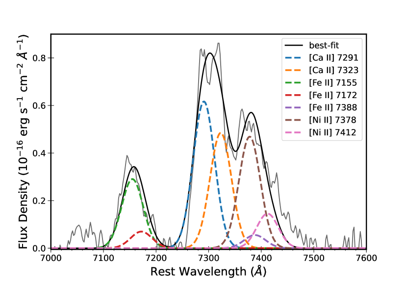
Figure 16: Section of the 365.2 day spectrum showing the Gaussian fits to determine [Ni II] $\lambda$7378/[Fe II] $\lambda$7155 in SN 2020jfo.

6.3 Bolometric light curve modelling

We constructed the bolometric light curve of SN 2020jfo using superbol (Nicholl, 2018) as shown in Figure 17. The dereddened magnitudes supplied to the routine are interpolated to a common set of epochs and converted to fluxes. The fluxes are used to construct the spectral energy distribution (SED) at all the epochs. The routine then fits a blackbody function to the SED, extrapolating to the UV and IR regimes to estimate the true bolometric luminosity. For SN 2020jfo, we used the Swift $uvw2$, $uvm2$, and $uvw1$ bands, optical $BgVri$ bands, and IR $J$-band data from Sollerman et al. (2021) to construct the first 50 days bolometric light curve using superbol. For the rest of the light curve, we used only $BgVri$ data.

We employed the semi-analytical modelling of Nagy & Vinkó (2016) to which an MCMC method was added by Jäger et al. (2020) for numerically fitting the output model to the observed light curves. Nagy & Vinkó (2016) used a core+shell combination to fit the early declining part with the shell configuration. The plateau phase, drop, and tail are modelled with the core configuration. However, the MCMC method added by Jäger et al. (2020) only takes into account the core part, and hence the early declining part (the first 10 days in the light curve) is not fitted using this method. For the modelling, we have sampled five parameters: radius ($R_{0}$), ejecta mass ($M_{\mathrm{ej}}$), kinetic energy ($E_{\mathrm{kin}}$), thermal energy ($E_{\mathrm{th}}$), and opacity. A mean and sigma prior expansion velocity of 8140 km s^-1 and 500 km s^-1 (respectively) were used, along with a recombination temperature of 5500 K. From the model, we estimated an initial radius ($R_{0}$) of $\sim 1000$ R_⊙, ejecta mass ($M_{\mathrm{ej}}$) of 13.6 M_⊙, and total energy ($E_{\mathrm{kin}}+E_{\mathrm{th}}$) of 3.0 foe. The bolometric magnitude evolution and the 50 best-fit light curves are shown in Figure 17, and the corresponding parameter estimates and their 1$\sigma$ uncertainties are provided in Table 5.

There are two known parameter correlations (Arnett & Fu, 1989; Nagy et al., 2014) between $M_{\mathrm{ej}}$ and $E_{\mathrm{kin}}$, and between $R_{0}$ and $E_{\mathrm{th}}$. Since the two parameter pairs $M_{\mathrm{ej}}-E_{\mathrm{kin}}$ and $E_{\mathrm{th}}-R_{0}$ are significantly correlated, separate determination of the quantities in the pair is not possible. Rather, the product of the pairs should be used as an independent parameter. The ⁵⁶Ni mass estimated from the modelling using the tail light curve is 0.022 M_⊙. Assuming a remnant neutron star mass of 1.5–2 M_⊙, the lower limit of the progenitor mass would be $\sim 15$ M_⊙, which lies within the expected mass range of RSGs exploding as Type IIP SNe. We note here that we could not reproduce the early luminosity excess by solely using the core component in the semi-analytical model. Thus, we cannot rule out the possibility of CSM interaction from pre-explosion mass loss.

In Inserra et al. (2013), hydrodynamic modelling of the bolometric light curve of SN 1995ad was performed, which estimated 5 M_⊙ of ejecta mass and a progenitor radius of $4\times 10^{13}$ cm. They proposed both super asymptotic giant branch (SAGB) and Fe CC progenitors, and noted that the former is less likely owing to the relatively high amount of ⁵⁶Ni ejected. The range of ejecta mass (5–7.5 M_⊙) and progenitor radius ((4–7) $\times 10^{13}$ cm) estimated for SN 2007od are also similar to SN 1995ad. In the work of Hiramatsu et al. (2021b), three short-plateau SNe 2006ai, 2006Y, and 2016egz were studied and the ZAMS mass ($M_{\rm ZAMS}$) of the progenitor was suggested to be in the range $\sim 18$–22 M_⊙, much higher than that of SNe 1995ad and 2007od. The study indicated that the progenitors of these SNe II had experienced massive stripping prior to explosion (Hiramatsu et al., 2021b), leading to a very low H-envelope mass ($\sim 1.7$ M_⊙), much lower than that of SNe 1995ad and 2005od. The ejecta mass estimated from semi-analytical modelling, which mainly constitutes the H-envelope mass, for SN 2020jfo is much higher than that of the SNe II studied by Inserra et al. (2013), Inserra et al. (2011), and Hiramatsu et al. (2021b). Although the early luminosity excess in SN 2020jfo and the high-velocity feature in H$\alpha$ indicate pre-explosion mass loss, the envelope stripping in the progenitor of SN 2020jfo is expectedly much less violent than in the Type II SNe 2006Y, 2006ai, and 2016egz.

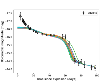
Figure 17: The bolometric magnitude evolution of SN 2020jfo is shown with the 50 best-fit light curves overplotted, following Nagy & Vinkó (2016) and Jäger et al. (2020).

Table 5: The best-fit core parameters and 1$\sigma$ confidence intervals for the bolometric light curve of SN 2020jfo using Nagy & Vinkó (2016).

$R_{0}$ ($10^{13}$ cm)	$6.89^{+0.45}_{-2.78}$	Initial radius of ejecta
$M_{\mathrm{ej}}$ (M⊙)	$13.6^{+0.2}_{-2.5}$	Ejecta mass
$E_{\mathrm{kin}}$ (foe)	$2.9^{+0.4}_{-0.5}$	Initial kinetic energy
$E_{\mathrm{th}}$ (foe)	$0.066^{+0.038}_{-0.004}$	Initial thermal energy

6.4 Metallicity

Metallicity is one of the key parameters that constrains the nature of the stellar evolution and the mechanism of the SN explosion, particularly in the case of high-mass stars (e.g., Heger et al. 2003). Pilyugin et al. (2004) derived an empirical relation between absolute $B$-magnitude ($M_{B}$) and metallicity (12 + log($N_{O}/N_{H}$)) for the nearby spiral galaxies (along with M61, the host of SN 2020jfo) and computed the radial profile of their metallicity distribution. The nuclear metallicity of M61 is 8.84 dex, and the angular separation between the SN and the host center is $\sim 1.2^{\prime}$. This implies that the metallicity at the SN location is roughly 8.57 dex (8.65 dex is the solar-neighbourhood metallicity; Asplund et al. 2009). Thus, the estimated metallicity of the region of SN 2020jfo using this method appears to be nearly solar, although it is higher than that of SN 2008in (8.44 dex; Roy et al. 2011b) which was located in the same host galaxy.

Metallicity also plays a crucial role in the evolution of metal lines in the photospheric phase as the SNe with low progenitor metallicity exhibit weaker metal features (Dessart et al., 2014). Dessart et al. (2013) simulated model spectra by evolving a 15 M_⊙ ZAMS star up to the pre-SN stage at various metallicities (0.1, 0.4, 1.0, 2.0 Z_⊙). We compared the day 80.2 spectrum of SN 2020jfo with these models and found a reasonable match with both 1 and 2 Z_⊙ model spectra considering the Fe II $\lambda$5018 and $\lambda$5169 features, that are overplotted on the spectrum of SN 2020jfo in the top panel of Figure 18. However, the higher metallicity model matches the H$\alpha$ absorption better. Furthermore, Anderson et al. (2016) estimated the oxygen abundances using a sample of 119 host H II regions and found a positive correlation between the host H II region oxygen abundance and the pseudo-equivalent width (pEW) of Fe II $\lambda$5018. In the bottom panel of Figure 18, the time evolution of the mean pEW of Fe II $\lambda$5018 of the sample of Type II SNe from Anderson et al. (2016) is shown along with its standard deviation (the black line and the shaded region), over which the thick solid lines are the time evolution of the pEW of Fe II $\lambda$5018 in the different metallicity models of Dessart et al. (2013). The pEW measurements of Fe II $\lambda$5018 in the spectra of SN 2020jfo is shown with a dashed line which falls slightly above the evolution of the 2 Z_⊙ model and is higher than the mean pEW of the sample. This estimate is higher than that obtained from radially decreasing metallicity gradients in spiral galaxies. Generally, higher metallicity would imply a higher extent of envelope stripping of the progenitor prior to explosion Heger et al. 2003. Despite the limitations of both methods of metallicity estimation, the higher metallicity scenario is more consistent with SNe II having shorter plateaus, where the progenitors are expected to have undergone comparatively extensive envelope stripping than Type II SNe with long plateaus (Hiramatsu et al., 2021b). In the context of SN 2020jfo, however, our analysis does not indicate significant envelope stripping. Thus, we prefer the low-luminosity scenario for SN 2020jfo.

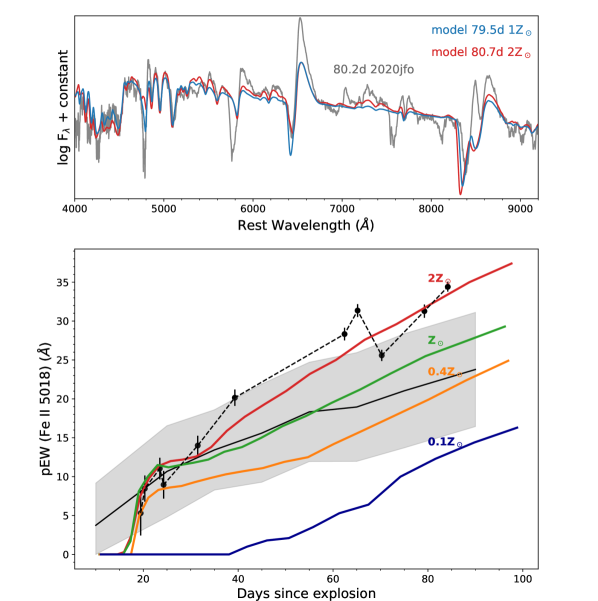
Figure 18: Top panel: Comparison of the day 80.2 spectrum of SN 2020jfo with the best-matched model spectrum of Dessart et al. (2013). Bottom panel: The evolution of the pEW of Fe II $\lambda$5018 of SN 2020jfo is shown with dashed lines. The black line is the mean pEW of a sample of 119 Type II SNe from (Anderson et al., 2016) and the shaded region shows the standard deviation about the mean. The time evolution of the pEWs of Fe II $\lambda$5018 of the four distinct metallicity models of (Dessart et al., 2013) is shown with thick lines.

7 Collocation of SN 2020jfo in the SN II parameter space

We explored the collocation of SN 2020jfo in the parameter space of other SNe II for which we have used the sample of Type II SNe from Anderson et al. (2014), Faran et al. (2014a), and Valenti et al. (2016b).

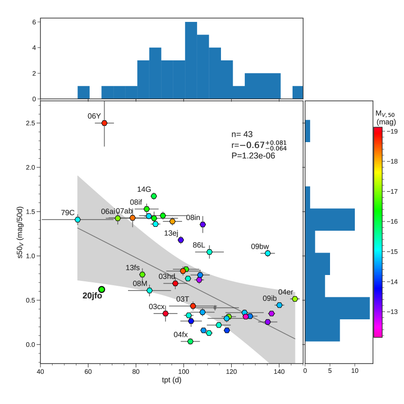
Figure 19: The correlation between $s50V$ and $t_{\rm pt}$ is shown. The objects are colour-coded with respect to the absolute $V$-band magnitude at day 50.

In Figure 19, the plateau decline rate in the $V$ band and $t_{\rm pt}$ of SN 2020jfo are shown colour-coded with the $V$ absolute magnitude at day 50, along with that of other SNe. There is a correlation among these parameters as noted by Valenti et al. (2016b). The correlation implies that SNe with longer plateaus tend to decline more slowly. The SNe with $t_{\rm pt}$ less than 80 days are SNe 1979C, 2006Y, and 2006ai. Although the plateau lengths of SNe 2006ai and 2006Y are consistent with SN 2020jfo within the uncertainties, SN 2006Y is brighter than SNe 2020jfo and 2006ai. We performed a linear fit and have shown the 3$\sigma$ confidence interval with the grey shaded region. SN 2006ai falls within the 3$\sigma$ confidence interval whereas SN 2020jfo falls outside it. Among the SNe with a short plateau duration, SN 2020jfo has the shallowest decline rate. In general, the SNe with shorter plateaus are brighter, with a higher decline rate than those with longer plateau. SNe with absolute plateau magnitudes in the range $-18$ to $-19$ mag are spread over all decline rates, while for the rest of the sample, SNe with lower luminosity preferably have shallower decline rates. SN 1979C is considered to be a prototypical Type IIL SN that does not show a clear light-curve drop. As suggested by Anderson et al. (2014), SN 1979C may have a light-curve drop around day 50 after explosion, though if there, the drop would have occurred quite early and less pronounced than in all the other cases.

We plot the absolute magnitude in $V$ at day 50 against the logarithm of the ⁵⁶Ni mass for a sample of Type II SNe. We find that the SNe II with higher luminosity (and hence higher explosion energy) have a larger ⁵⁶Ni yield. SN 2020jfo follows the correlation between these two parameters. Also, we plot peak magnitude in $V$ against $a_{0}$ of SN 2020jfo along with those of other Type II SNe. In general, SNe with higher peak magnitudes have shorter plateau lengths. Hence, the fall in magnitude from the plateau to the radioactive tail phase is expected to be lower. SN 2020jfo follows the trend, but the plateau length of SN 2020jfo is shorter and slowly declining compared with other short-plateau SNe.

The correlations suggest that although SN 2020jfo has a short plateau length, its parameters are more similar to those of normal SNe IIP.

8 Conclusions

In this paper, we present a photometric and spectroscopic analysis of the Type II SN 2020jfo. Using the light-curve equation from Valenti et al. (2016b), we estimated a short-plateau length of $67.0\pm 0.6$ days for SN 2020jfo, which is consistent with the result given by Sollerman et al. (2021) and Singh Teja et al. (2022).

However, unlike other SNe II with shorter plateau duration, SN 2020jfo is fainter, with a peak absolute $V$-band magnitude of $-16.90\pm 0.34$ mag, in comparison with the luminous optical peaks of those SNe ($\lesssim-18.4$ mag). While the plateau decline rates in $V$ of SN 2020jfo and other SNe II having shorter plateau duration are similar, the short-plateau Type II SNe 1995ad, 2006Y, 2006ai, 2007od, and 2016egz display a steeply declining phase in $V$ up to $\sim 20$ days, which is not observed in SN 2020jfo. The ⁵⁶Ni mass yield of SN 2020jfo estimated from the tail-phase luminosity is $0.03\pm 0.01$ $M_{\odot}$, which falls in the range of normal SNe II.

Despite the shorter plateau duration in SN 2020jfo, the H I absorption features in its plateau-phase spectra are remarkably strong, indicating a relatively high H-envelope mass. SN 2020jfo also shows strong metal lines in comparison with other SNe II at similar epochs and having comparable plateau lengths. Moreover, a discernible line of stable [Ni II] $\lambda$7378, which has only been seen in a few H-rich SNe, could be identified in the nebular spectra of SN 2020jfo. Analysis of the line ratio of [Ni II] $\lambda$7378 to [Fe II] $\lambda$7155 suggests a supersolar Ni-to-Fe production ratio by mass.

From nebular-phase spectral comparison (Jerkstrand et al., 2014), we estimated the ZAMS mass of the progenitor of SN 2020jfo to be around 12 M_⊙. Moreover, semi-analytical modelling using the prescription of Nagy & Vinkó (2016) indicated an ejecta mass of $13.6^{+0.2}_{-2.5}$ M_⊙. Adding a remnant neutron star mass, the progenitor mass turns out to be $15^{+0.2}_{-2.5}$ M_⊙. This can be considered as a lower limit of the progenitor ZAMS mass, since the analytical method does not estimate the mass lost by winds. The SN 2020jfo ejecta mass estimated from semi-analytical modelling, which mainly constitutes the H-envelope mass, is much higher than that of the Type II SNe studied by Inserra et al. (2013), Inserra et al. (2011), and Hiramatsu et al. (2021b) with similar plateau lengths. Thus, spectroscopic comparison and modelling suggests that SN 2020jfo differs from SNe II with similar plateau lengths and is rather spectroscopically similar to SN 1999em.

Data Availability

The photometric and spectroscopic data underlying this article will be made available upon request to the corresponding author.

Appendix A Data tables

Table 6: Swift/UVOT photometry of SN 2020jfo^a

Date	Phaseb	$uw2$	$um2$	$uw1$	$uvu$	$uvb$	$uvv$
(UT)	(days)	(mag)	(mag)	(mag)	(mag)	(mag)	(mag)
2020-05-07.13	3.52	14.75$\pm$ 0.09	14.75$\pm$ 0.06	14.64$\pm$ 0.08	14.55$\pm$ 0.06	14.74$\pm$ 0.05	14.99$\pm$0.06
2020-05-08.73	5.13	14.81$\pm$ 0.09	14.66$\pm$ 0.07	14.60$\pm$ 0.08	14.40$\pm$ 0.06	14.53$\pm$ 0.05	14.62$\pm$0.06
2020-05-09.23	5.63	15.18$\pm$ 0.09	14.86$\pm$ 0.06	14.79$\pm$ 0.08	14.42$\pm$ 0.06	14.58$\pm$ 0.05	14.62$\pm$0.06
2020-05-10.35	6.75	15.39$\pm$ 0.09	15.08$\pm$ 0.07	14.87$\pm$ 0.08	14.40$\pm$ 0.06	14.48$\pm$ 0.05	14.54$\pm$0.06
2020-05-10.42	6.82	15.47$\pm$ 0.09	15.12$\pm$ 0.07	14.97$\pm$ 0.08	14.48$\pm$ 0.06	14.53$\pm$ 0.06	14.58$\pm$0.07
2020-05-11.22	7.62	15.76$\pm$ 0.09	15.34$\pm$ 0.06	14.96$\pm$ 0.08	14.41$\pm$ 0.06	14.49$\pm$ 0.05	14.51$\pm$0.06
2020-05-12.76	9.15	16.31$\pm$ 0.09	15.91$\pm$ 0.07	15.36$\pm$ 0.08	14.54$\pm$ 0.06	14.59$\pm$ 0.05	14.58$\pm$0.06
2020-05-13.42	9.81	16.33$\pm$ 0.09	16.05$\pm$ 0.07	15.48$\pm$ 0.08	14.57$\pm$ 0.06	14.52$\pm$ 0.05	14.58$\pm$0.06
2020-05-15.67	12.07	16.83$\pm$ 0.10	16.73$\pm$ 0.07	15.95$\pm$ 0.08	14.78$\pm$ 0.06	14.58$\pm$ 0.06	14.75$\pm$0.07
2020-05-16.66	13.06	17.17$\pm$ 0.10	17.05$\pm$ 0.08	16.18$\pm$ 0.09	14.84$\pm$ 0.06	14.66$\pm$ 0.06	14.73$\pm$0.07
2020-05-24.91	21.31	19.93$\pm$ 0.12	19.90$\pm$ 0.10	18.20$\pm$ 0.10	16.23$\pm$ 0.07	14.96$\pm$ 0.06	14.66$\pm$0.06
2020-05-26.56	22.95	19.78$\pm$ 0.12	20.20$\pm$ 0.10	18.53$\pm$ 0.11	16.62$\pm$ 0.07	15.04$\pm$ 0.06	14.71$\pm$0.06
2020-06-02.76	30.16	20.89$\pm$ 0.11	21.34$\pm$ 0.09	19.30$\pm$ 0.10	17.33$\pm$ 0.07	15.45$\pm$ 0.05	14.79$\pm$0.06
2020-06-07.11	34.5	20.60$\pm$ 0.10	21.24$\pm$ 0.08	19.51$\pm$ 0.09	17.71$\pm$ 0.07	15.57$\pm$ 0.05	14.86$\pm$0.05
2020-06-13.09	40.48	21.19$\pm$ 0.11	21.79$\pm$ 0.09	19.96$\pm$ 0.10	18.12$\pm$ 0.08	15.72$\pm$ 0.05	14.93$\pm$0.06
2020-06-18.00	45.39	22.29$\pm$ 0.15	20.90$\pm$ 0.12	19.66$\pm$ 0.14	18.65$\pm$ 0.13	15.90$\pm$ 0.07	14.91$\pm$0.07
2020-07-18.41	75.81	21.50$\pm$ 0.10	22.63$\pm$ 0.08	21.83c	20.79	18.58$\pm$ 0.07	17.51$\pm$0.08
2020-07-29.33	86.72	21.74$\pm$ 0.10	21.74$\pm$ 0.08	21.82$\pm$ 0.10	20.52	18.71$\pm$ 0.07	17.28$\pm$0.07
2020-08-03.41	91.81	21.72$\pm$ 0.10	21.48$\pm$ 0.08	21.63$\pm$ 0.10	20.60	19.00$\pm$ 0.07	17.53$\pm$0.08
2020-08-08.45	96.9	21.73$\pm$ 0.10	22.14	21.61	21.49$\pm$ 0.09	18.86$\pm$ 0.07	17.47$\pm$0.10
2020-11-14.65	195.0	21.86	22.69$\pm$ 0.10	21.87$\pm$ 0.10	20.28	20.28$\pm$ 0.09	18.58$\pm$0.15
2020-12-12.03	222.43	21.64$\pm$ 0.11	22.05$\pm$ 0.08	21.67	21.24$\pm$ 0.09	21.11$\pm$ 0.08	19.25$\pm$0.11
2020-12-24.41	234.81	22.94	22.14$\pm$ 0.07	22.17	21.12	21.41$\pm$ 0.07	19.55$\pm$0.08
2021-01-13.53	254.92	22.98	22.99	22.24	21.18	20.37	20.08$\pm$0.08
2021-01-28.99	270.39	22.31$\pm$ 0.14	21.63	20.99	20.03	19.29	20.95$\pm$0.18
2021-01-30.53	271.92	22.80	22.83	22.13	21.10	20.31	20.47$\pm$0.09

^aThe magnitudes of the transient have been determined after subtracting the host flux at the SN location from recent photometry. The host flux at the SN location in different UVOT bands has been determined from previous Swift observations (in the year 2008) of the field (see the text for details).
^bPhase with respect to the explosion epoch (MJD = 58973.1).
^cMagnitudes without uncertainties correspond to upper limits.

Table 7: Details of the instruments used for the observational campaign of SN 2020jfo.

Telescope	Location	Instrument	Pixel Scale	Imaging	Dispersers/
			("/pixel)	bands	Grisms
0.76m KAIT	Lick Observatory	-	0.80	$BVRI$
1.04m ST	ARIES Observatory, India	Tek 1k $\times$ 1k	0.53	$BVRI$	-
1.0m Nickel	Lick Observatory	-	0.184	BVRI
1.0m LCO	Siding Spring Observatory	Sinistro	0.389	$BVg^{\prime}r^{\prime}i^{\prime}$	-
1.0m LCO	South African	Sinistro	0.389	$BVg^{\prime}r^{\prime}i^{\prime}$	-
	Astronomical Observatory
1.0m LCO	McDonald Observatory	Sinistro	0.389	$BVg^{\prime}r^{\prime}i^{\prime}$	-
1.0m LCO	Cerro Tololo	Sinistro	0.389	$BVg^{\prime}r^{\prime}i^{\prime}$	-
	Interamerican Observatory
1.3m DFOT	ARIES Observatory, India	Andor $512\times 512$	0.64	$UBVRI$	-
2.0m FTN	Haleakala Observatory, USA	Spectral, FLOYDS	0.304, 0.34	-	Cross disperser
2.0m FTS	Siding Spring Observatory,	FLOYDS	0.34	-	Cross disperser
	Australia
3.0m NASA IRTF	Mauna Kea	SpeX	0.15	-	Cross disperser
3.0m Shane	Lick Observatory	Kast	0.43	-	-
3.6m DOT	ARIES Observatory, India	ADFOSC	-	-	-
10.4m GTC	La Palma, Spain	OSIRIS	0.254	-	R1000B, R1000R

Table 8: Optical photometry of SN 2020jfo with LCO network of telescopes

Date	Phasea	$B$	$V$	$g$	$r$	$i$
(UT)	(days)	(mag)	(mag)	(mag)	(mag)	(mag)
2020-05-06.90	2.80				15.16$\pm$0.06b
2020-05-07.51	3.41	14.78$\pm$0.08	14.77$\pm$0.09	14.61$\pm$0.11	15.02$\pm$0.05	15.07$\pm$0.12
2020-05-07.76	3.66	14.76$\pm$0.06	14.76$\pm$0.02	14.60$\pm$0.06	14.91$\pm$0.08	14.96$\pm$0.08
2020-05-08.44	4.34	14.67$\pm$0.02	14.63$\pm$0.03	14.66$\pm$0.50	14.67$\pm$0.10	14.86$\pm$0.01
2020-05-09.54	5.44	15.01$\pm$0.08	-	14.57$\pm$0.01	14.61$\pm$0.01	14.55$\pm$0.01
2020-05-10.36	6.26	14.54$\pm$0.02	-	14.38$\pm$0.01	14.42$\pm$0.04	14.55$\pm$0.04
2020-05-10.87	6.77	14.63$\pm$0.02	14.44$\pm$0.14	14.48$\pm$0.02	14.43$\pm$0.06	14.45$\pm$0.06
2020-05-11.56	7.46	14.61$\pm$0.05	14.47$\pm$0.06	14.23$\pm$0.02	14.37$\pm$0.04	14.51$\pm$0.04
2020-05-12.37	8.27	14.57$\pm$0.01	14.44$\pm$0.02	14.45$\pm$0.05	14.45$\pm$0.03	14.56$\pm$0.08
2020-05-12.85	8.75	14.67$\pm$0.03	14.53$\pm$0.02	14.49$\pm$0.04	14.56$\pm$0.06	14.49$\pm$0.30
2020-05-13.81	9.71	14.72$\pm$0.03	14.60$\pm$0.02	14.57$\pm$0.06	14.53$\pm$0.01	14.57$\pm$0.08
2020-05-14.83	10.73	14.82$\pm$0.04	14.53$\pm$0.02	14.55$\pm$0.01	14.60$\pm$0.01	14.69$\pm$0.02
2020-05-17.81	13.71	14.90$\pm$0.02	14.43$\pm$0.02	14.50$\pm$0.09	14.55$\pm$0.01	14.58$\pm$0.10
2020-05-19.35	15.25	14.98$\pm$0.12	15.29$\pm$0.04	13.32$\pm$0.11	14.81$\pm$0.02	14.85$\pm$0.38
2020-05-20.74	16.64	15.01$\pm$0.04	14.56$\pm$0.02	14.68$\pm$0.01	14.54$\pm$0.01	14.72$\pm$0.01
2020-05-24.84	20.74	15.25$\pm$0.02	14.59$\pm$0.02	14.80$\pm$0.01	14.62$\pm$0.01	14.67$\pm$0.01
2020-05-27.70	23.60	15.31$\pm$0.05	14.68$\pm$0.02	14.82$\pm$0.09	14.59$\pm$0.01	14.60$\pm$0.06
2020-05-29.70	25.60	15.45$\pm$0.05	14.63$\pm$0.02	14.96$\pm$0.02	14.58$\pm$0.01	14.61$\pm$0.01
2020-06-04.85	31.75	15.67$\pm$0.02	14.72$\pm$0.02	15.12$\pm$0.01	14.65$\pm$0.01	14.63$\pm$0.01
2020-06-09.75	36.65	15.83$\pm$0.02	14.78$\pm$0.02	15.23$\pm$0.01	14.80$\pm$0.01	14.74$\pm$0.01
2020-06-15.41	42.31	16.02$\pm$0.02	14.92$\pm$0.02	15.39$\pm$0.01	14.74$\pm$0.01	14.69$\pm$0.01
2020-06-19.45	46.35	15.99$\pm$0.02	14.80$\pm$0.02	15.43$\pm$0.01	14.68$\pm$0.01	14.57$\pm$0.01
2020-06-30.40	57.30	16.62$\pm$0.02	15.26$\pm$0.02	15.76$\pm$0.01	-	14.93$\pm$0.02
2020-07-03.80	60.70	16.75$\pm$0.02	15.29$\pm$0.02	15.93$\pm$0.01	14.99$\pm$0.01	14.91$\pm$0.01
2020-07-08.76	65.67	17.46$\pm$0.02	15.79$\pm$0.02	16.64$\pm$0.01	15.42$\pm$0.01	15.35$\pm$0.01
2020-07-15.73	72.63	18.81$\pm$0.03	16.99$\pm$0.02	17.89$\pm$0.01	16.49$\pm$0.01	16.49$\pm$0.01
2020-07-18.76	75.66	18.81$\pm$0.03	-	-	-	-
2020-07-20.71	77.61	19.00$\pm$0.02	17.28$\pm$0.02	17.97$\pm$0.01	16.61$\pm$0.01	16.58$\pm$0.01
2020-07-23.74	80.64	18.68$\pm$0.02	17.11$\pm$0.03	17.77$\pm$0.02	16.51$\pm$0.01	16.49$\pm$0.02
2020-07-27.76	84.66	18.84$\pm$0.14	17.37$\pm$0.06	17.72$\pm$0.01	16.47$\pm$0.02	16.71$\pm$0.03
2020-07-31.38	88.28	-	17.78$\pm$0.39	-	17.17$\pm$0.18	17.13$\pm$0.35
2020-08-05.74	93.64	18.70$\pm$0.06	17.30$\pm$0.04	18.03$\pm$0.03	16.58$\pm$0.02	16.90$\pm$0.03
2020-08-10.37	98.27	18.51$\pm$0.09	17.41$\pm$0.09	17.83$\pm$0.03	16.59$\pm$0.04	16.91$\pm$0.03
2020-12-19.48	229.38	20.04$\pm$0.06	19.03$\pm$0.04	19.35$\pm$0.03	18.45$\pm$0.02	18.53$\pm$0.04
2020-12-23.45	233.35	20.16$\pm$0.07	19.12$\pm$0.08	19.44$\pm$0.03	18.61$\pm$0.02	18.91$\pm$0.05
2021-01-03.50	244.40	20.57$\pm$0.10	19.57$\pm$0.10	19.85$\pm$0.08	18.97$\pm$0.06	19.09$\pm$0.13
2021-01-15.07	255.97	20.44$\pm$0.08	19.41$\pm$0.06	19.54$\pm$0.03	19.12$\pm$0.04	18.85$\pm$0.06
2021-01-26.08	266.98	20.57$\pm$0.08	19.54$\pm$0.07	19.84$\pm$0.03	19.62$\pm$0.04	19.46$\pm$0.03
2021-02-06.08	277.98	20.90$\pm$0.11	19.68$\pm$0.06	-	19.66$\pm$0.05	-
2021-02-09.34	281.24	21.20$\pm$0.16	19.83$\pm$0.06	19.92$\pm$0.04	19.72$\pm$0.06	19.39$\pm$0.07
2021-02-27.66	299.56	21.08$\pm$0.14	20.28$\pm$0.08	19.92$\pm$0.05	20.33$\pm$0.08	19.80$\pm$0.07
2021-03-11.23	311.13	21.69$\pm$0.28	20.32$\pm$0.09	20.29$\pm$0.05	20.46$\pm$0.13	19.85$\pm$0.08
2021-03-22.24	322.14	21.63$\pm$0.30	20.51$\pm$0.09	20.46$\pm$0.06	20.79$\pm$0.15	20.09$\pm$0.07
2021-04-03.95	334.85	22.24$\pm$0.34	20.66$\pm$0.14	20.58$\pm$0.06	21.44$\pm$0.18	20.56$\pm$0.13
2021-04-14.89	345.79	22.50$\pm$0.45	20.66$\pm$0.13	20.61$\pm$0.07	21.49$\pm$0.19	20.47$\pm$0.19
2021-04-27.18	358.08	21.53$\pm$0.13	21.60$\pm$0.39	-	-	20.88$\pm$0.38
2021-05-08.18	369.08	22.61$\pm$0.38	21.07$\pm$0.18	21.43$\pm$0.39	-	-
2021-05-13.36	374.26	-	21.03$\pm$0.15	-	-	-
2021-05-24.50	385.40	22.00$\pm$0.38	21.51$\pm$0.32	22.05$\pm$0.22	21.38$\pm$0.40	20.28$\pm$0.22
2021-06-04.71	396.61	-	21.18$\pm$0.21	21.64$\pm$0.16	-	-
2021-06-06.41	398.31	-	21.34$\pm$0.24	21.30$\pm$0.12	21.92$\pm$0.28	21.48$\pm$0.44
2021-06-21.06	412.96	22.68$\pm$0.51	22.50$\pm$0.43	-	21.83$\pm$0.23	21.15$\pm$0.23
2021-07-02.04	423.94	-	21.53$\pm$0.31	21.91$\pm$0.26	22.01$\pm$0.34	-
2021-07-13.00	434.90	-	-	21.52$\pm$0.50	-	-

^aPhase with respect to the explosion epoch (MJD = 58973.1).
^bThe earliest photometric data obtained with the 10.4 m GTC.

Table 9: Optical photometry of SN 2020jfo with ARIES telescopes

Date	Phasea	$B$	$V$	$R$	$I$
(UT)	(days)	(mag)	(mag)	(mag)	(mag)
2021-01-06.98	248.37	$-$	19.26$\pm$0.05	19.09$\pm$0.09	19.89$\pm$0.17
2021-01-07.90	249.30	19.78$\pm$0.09	19.20$\pm$0.06	19.31$\pm$0.09	19.55$\pm$0.20
2021-01-07.91	249.31	$-$	19.19$\pm$0.05	19.50$\pm$0.06	19.49$\pm$0.16
2021-01-09.90	251.26	20.14$\pm$0.21	19.21$\pm$0.05	19.20$\pm$0.08	19.66$\pm$0.16
2021-01-21.96	263.34	20.07$\pm$0.19	19.11$\pm$0.06	18.84$\pm$0.08	19.97$\pm$0.28
2021-02-02.98	275.38	20.4	19.77$\pm$0.14	18.81$\pm$0.10	19.86$\pm$0.27
2021-02-14.79	287.19	20.59$\pm$0.23	20.16$\pm$0.09	18.90$\pm$0.08	19.98$\pm$0.17
2021-02-22.81	295.37	21.21$\pm$0.32	20.17$\pm$0.10	19.67$\pm$0.13	21.12$\pm$0.32

^aPhase with respect to the explosion epoch (MJD = 58973.1).
^bMagnitude without error corresponds to the upper limit.

Table 10: Optical photometry of SN 2020jfo with Lick Observatory telescopes

Date	Phasea	$B$	$V$	$R$	$I$	Clear
(UT)	(days)	(mag)	(mag)	(mag)	(mag)	(mag)
2020-05-07.32	3.22	14.66$\pm$0.06	15.01$\pm$0.03	14.94$\pm$0.06	14.96$\pm$0.06	14.78$\pm$0.04
2020-05-08.35	4.25	14.58$\pm$0.04	14.77$\pm$0.02	14.71$\pm$0.02	14.64$\pm$0.03	14.55$\pm$0.03
2020-05-09.25	5.15	14.52$\pm$0.04	14.66$\pm$0.02	14.58$\pm$0.02	14.47$\pm$0.02	14.44$\pm$0.03
2020-05-10.34	6.24	14.54$\pm$0.05	14.63$\pm$0.02	14.48$\pm$0.02	14.37$\pm$0.03	14.38$\pm$0.02
2020-05-11.30	7.20	14.48$\pm$0.05	14.59$\pm$0.03	14.45$\pm$0.02	14.31$\pm$0.03	14.37$\pm$0.02
2020-05-16.27	12.17	14.66$\pm$0.03	14.71$\pm$0.01	14.51$\pm$0.01	14.45$\pm$0.02	14.44$\pm$0.02
2020-05-17.27	13.17	14.68$\pm$0.05	14.76$\pm$0.04	14.50$\pm$0.04	14.42$\pm$0.10	14.46$\pm$0.02
2020-05-21.24	17.14	14.79$\pm$0.08	14.66$\pm$0.02	14.48$\pm$0.02	14.37$\pm$0.03	-
2020-05-21.31	17.21	14.87$\pm$0.04	14.73$\pm$0.02	14.51$\pm$0.02	14.43$\pm$0.03	14.46$\pm$0.03
2020-05-23.25	19.15	14.94$\pm$0.04	14.71$\pm$0.02	14.50$\pm$0.02	14.38$\pm$0.02	14.48$\pm$0.03
2020-05-24.27	20.17	15.01$\pm$0.04	14.73$\pm$0.02	14.50$\pm$0.02	14.39$\pm$0.03	14.49$\pm$0.03
2020-05-25.28	21.18	15.00$\pm$0.08	14.77$\pm$0.02	14.52$\pm$0.02	14.41$\pm$0.02	14.49$\pm$0.03
2020-05-26.25	22.15	15.10$\pm$0.04	14.75$\pm$0.02	14.51$\pm$0.02	14.38$\pm$0.03	14.51$\pm$0.02
2020-05-27.25	23.15	15.14$\pm$0.04	14.77$\pm$0.02	14.53$\pm$0.02	14.41$\pm$0.03	14.52$\pm$0.03
2020-05-28.26	24.16	15.20$\pm$0.04	14.78$\pm$0.02	14.52$\pm$0.02	14.37$\pm$0.02	14.55$\pm$0.03
2020-06-02.18	29.08	15.39$\pm$0.09	14.78$\pm$0.08	14.54$\pm$0.13	14.26$\pm$0.10	-
2020-06-02.24	29.14	15.35$\pm$0.09	14.76$\pm$0.03	14.54$\pm$0.02	14.34$\pm$0.03	-
2020-06-04.27	31.17	15.50$\pm$0.05	14.83$\pm$0.02	14.56$\pm$0.02	14.38$\pm$0.03	14.60$\pm$0.02
2020-06-06.26	33.16	15.47$\pm$0.13	14.79$\pm$0.06	14.54$\pm$0.02	14.32$\pm$0.04	-
2020-06-10.21	37.11	15.67$\pm$0.08	14.86$\pm$0.03	14.59$\pm$0.02	14.35$\pm$0.03	-
2020-06-14.24	41.14	15.74$\pm$0.08	14.88$\pm$0.03	14.60$\pm$0.02	14.36$\pm$0.03	-
2020-06-18.24	45.14	15.91$\pm$0.23	14.92$\pm$0.14	14.65$\pm$0.02	14.38$\pm$0.04	-
2020-06-22.25	49.15	16.05$\pm$0.08	14.97$\pm$0.03	14.66$\pm$0.02	14.42$\pm$0.25	-
2020-06-30.20	57.10	16.27$\pm$0.08	15.20$\pm$0.03	14.82$\pm$0.02	14.55$\pm$0.04	-
2020-06-30.24	57.14	16.27$\pm$0.07	15.23$\pm$0.03	14.84$\pm$0.03	14.57$\pm$0.03	14.88$\pm$0.04
2020-07-01.21	58.11	16.34$\pm$0.07	15.29$\pm$0.03	14.91$\pm$0.03	14.63$\pm$0.04	14.99$\pm$0.04
2020-07-04.23	61.13	16.58$\pm$0.08	15.43$\pm$0.02	14.97$\pm$0.02	14.71$\pm$0.03	15.08$\pm$0.04
2020-07-05.20	62.10	16.78$\pm$0.10	15.57$\pm$0.03	15.08$\pm$0.03	14.78$\pm$0.03	15.20$\pm$0.04
2020-07-08.22	65.12	17.16$\pm$0.09	15.83$\pm$0.04	15.30$\pm$0.03	15.00$\pm$0.04	15.45$\pm$0.05
2020-07-10.20	67.10	17.44$\pm$0.13	16.18$\pm$0.05	15.57$\pm$0.05	15.30$\pm$0.05	15.76$\pm$0.06
2020-07-11.22	68.12	17.68$\pm$0.15	16.43$\pm$0.05	15.76$\pm$0.04	15.45$\pm$0.05	15.91$\pm$0.07
2020-07-18.20	75.10	-	-	-	-	16.55$\pm$0.20
2020-07-19.20	76.10	17.96$\pm$0.24	17.20$\pm$0.10	16.43$\pm$0.08	16.06$\pm$0.07	16.53$\pm$0.12
2020-07-20.20	77.10	-	-	-	-	16.49$\pm$0.13
2020-07-21.20	78.10	18.20$\pm$0.28	17.14$\pm$0.10	16.41$\pm$0.07	16.10$\pm$0.07	16.52$\pm$0.11
2020-07-23.20	80.10	18.26$\pm$0.38	17.18$\pm$0.15	16.37$\pm$0.11	16.15$\pm$0.09	16.55$\pm$0.14

^a Phase with respect to the explosion epoch (MJD = 58973.1).

Table 11: Spectroscopic log of SN 2020jfo

Date	Phasea	Telescope
(UT)	(days)
	Optical
2020-05-06.90	2.80	GTC
2020-05-07.54	3.44	FTS
2020-05-08.55	4.45	FTS
2020-05-12.36	8.26	FTN
2020-05-16.49	12.39	FTS
2020-05-17.27	13.17	Shane
2020-05-19.50	15.40	FTS
2020-05-23.00	18.90	DOT
2020-05-24.00	19.90	DOT
2020-05-24.46	20.36	FTS
2020-05-25.33	21.17	Shane
2020-05-28.48	24.38	FTS
2020-05-29.29	25.19	Shane
2020-06-05.48	32.38	FTS
2020-06-13.30	40.20	FTN
2020-06-26.27	53.17	FTN
2020-07-06.42	63.32	FTS
2020-07-09.20	66.10	Shane
2020-07-14.26	71.16	FTN
2020-07-18.20	75.09	Shane
2020-07-23.25	80.15	FTN
2020-07-28.19	85.09	Shane
2020-08-01.35	89.25	FTS
2021-01-13.00	253.90	DOT
2021-01-15.00	255.90	DOT
2021-05-04.30	365.20	Shane
	NIR
2020-05-13	9.27	IRTF
2020-05-24	20.24	IRTF
2020-06-15	42.19	IRTF

^a Phase with respect to the explosion epoch (MJD = 58973.1).

References

- Anderson et al. (2014) Anderson J. P., et al., 2014, MNRAS, 441, 671
- Anderson et al. (2016) Anderson J. P., et al., 2016, A&A, 589, A110
- Arnett & Fu (1989) Arnett W. D., Fu A., 1989, ApJ, 340, 396
- Asplund et al. (2009) Asplund M., Grevesse N., Sauval A. J., Scott P., 2009, ARA&A, 47, 481
- Barbarino et al. (2015) Barbarino C., et al., 2015, MNRAS, 448, 2312
- Barbon et al. (1979) Barbon R., Ciatti F., Rosino L., 1979, A&A, 72, 287
- Bellm et al. (2019) Bellm E. C., et al., 2019, PASP, 131, 068003
- Benetti et al. (2001) Benetti S., et al., 2001, MNRAS, 322, 361
- Blondin & Tonry (2007) Blondin S., Tonry J. L., 2007, ApJ, 666, 1024
- Bose & Kumar (2014) Bose S., Kumar B., 2014, ApJ, 782, 98
- Bose et al. (2013) Bose S., et al., 2013, MNRAS, 433, 1871
- Bose et al. (2015a) Bose S., et al., 2015a, MNRAS, 450, 2373
- Bose et al. (2015b) Bose S., et al., 2015b, ApJ, 806, 160
- Bose et al. (2016) Bose S., Kumar B., Misra K., Matsumoto K., Kumar B., Singh M., Fukushima D., Kawabata M., 2016, MNRAS, 455, 2712
- Bose et al. (2019) Bose S., et al., 2019, ApJ, 873, L3
- Brown et al. (2009) Brown P. J., et al., 2009, AJ, 137, 4517
- Chugai & Utrobin (2000) Chugai N. N., Utrobin V. P., 2000, A&A, 354, 557
- Cushing et al. (2004) Cushing M. C., Vacca W. D., Rayner J. T., 2004, PASP, 116, 362
- Dall’Ora et al. (2014) Dall’Ora M., et al., 2014, ApJ, 787, 139
- Dastidar et al. (2018) Dastidar R., et al., 2018, MNRAS, 479, 2421
- Davis et al. (2019) Davis S., et al., 2019, ApJ, 887, 4
- Dessart & Hillier (2005) Dessart L., Hillier D. J., 2005, A&A, 439, 671
- Dessart et al. (2008) Dessart L., et al., 2008, ApJ, 675, 644
- Dessart et al. (2013) Dessart L., Waldman R., Livne E., Hillier D. J., Blondin S., 2013, MNRAS, 428, 3227
- Dessart et al. (2014) Dessart L., Blondin S., Hillier D. J., Khokhlov A., 2014, MNRAS, 441, 532
- Elmhamdi et al. (2003) Elmhamdi A., et al., 2003, MNRAS, 338, 939
- Elmhamdi et al. (2004) Elmhamdi A., Danziger I. J., Cappellaro E., Della Valle M., Gouiffes C., Phillips M. M., Turatto M., 2004, A&A, 426, 963
- Faran et al. (2014a) Faran T., et al., 2014a, MNRAS, 442, 844
- Faran et al. (2014b) Faran T., et al., 2014b, MNRAS, 445, 554
- Filippenko (1988) Filippenko A. V., 1988, AJ, 96, 1941
- Filippenko (1997) Filippenko A. V., 1997, ARA&A, 35, 309
- Filippenko et al. (2001) Filippenko A. V., Li W. D., Treffers R. R., Modjaz M., 2001, in Paczynski B., Chen W.-P., Lemme C., eds, Astronomical Society of the Pacific Conference Series Vol. 246, IAU Colloq. 183: Small Telescope Astronomy on Global Scales. p. 121
- Fransson & Chevalier (1989) Fransson C., Chevalier R. A., 1989, ApJ, 343, 323
- Goldberg et al. (2019) Goldberg J. A., Bildsten L., Paxton B., 2019, ApJ, 879, 3
- Graham et al. (2019) Graham M. J., et al., 2019, PASP, 131, 078001
- Gutiérrez et al. (2017) Gutiérrez C. P., et al., 2017, ApJ, 850, 89
- Hamuy (2003) Hamuy M., 2003, ApJ, 582, 905
- Hamuy et al. (2001a) Hamuy M., et al., 2001a, ApJ, 558, 615
- Hamuy et al. (2001b) Hamuy M., et al., 2001b, ApJ, 558, 615
- Heger et al. (2003) Heger A., Fryer C. L., Woosley S. E., Langer N., Hartmann D. H., 2003, ApJ, 591, 288
- Hiramatsu et al. (2021a) Hiramatsu D., et al., 2021a, Nature Astronomy, 5, 903
- Hiramatsu et al. (2021b) Hiramatsu D., et al., 2021b, ApJ, 913, 55
- Hosseinzadeh & Gomez (2020) Hosseinzadeh G., Gomez S., 2020, Light Curve Fitting, doi:10.5281/zenodo.4312178, https://doi.org/10.5281/zenodo.4312178
- Hosseinzadeh et al. (2018) Hosseinzadeh G., et al., 2018, ApJ, 861, 63
- Inserra et al. (2011) Inserra C., et al., 2011, MNRAS, 417, 261
- Inserra et al. (2012) Inserra C., Baron E., Turatto M., 2012, MNRAS, 422, 1178
- Inserra et al. (2013) Inserra C., et al., 2013, A&A, 555, A142
- Jäger et al. (2020) Jäger Zoltán J., et al., 2020, MNRAS, 496, 3725
- Jerkstrand et al. (2012) Jerkstrand A., Fransson C., Maguire K., Smartt S., Ergon M., Spyromilio J., 2012, A&A, 546, A28
- Jerkstrand et al. (2014) Jerkstrand A., Smartt S. J., Fraser M., Fransson C., Sollerman J., Taddia F., Kotak R., 2014, MNRAS, 439, 3694
- Jerkstrand et al. (2015) Jerkstrand A., et al., 2015, ApJ, 807, 110
- Kasen & Woosley (2009) Kasen D., Woosley S. E., 2009, ApJ, 703, 2205
- Kuncarayakti et al. (2015) Kuncarayakti H., et al., 2015, A&A, 579, A95
- Leonard et al. (2002) Leonard D. C., et al., 2002, PASP, 114, 35
- Leonard et al. (2003) Leonard D. C., Kanbur S. M., Ngeow C. C., Tanvir N. R., 2003, ApJ, 594, 247
- Müller-Bravo et al. (2020) Müller-Bravo T. E., et al., 2020, MNRAS, 497, 361
- Müller et al. (2017) Müller T., Prieto J. L., Pejcha O., Clocchiatti A., 2017, ApJ, 841, 127
- Nadyozhin (2003) Nadyozhin D. K., 2003, MNRAS, 346, 97
- Nagy & Vinkó (2016) Nagy A. P., Vinkó J., 2016, A&A, 589, A53
- Nagy et al. (2014) Nagy A. P., Ordasi A., Vinkó J., Wheeler J. C., 2014, A&A, 571, A77
- Nicholl (2018) Nicholl M., 2018, Research Notes of the American Astronomical Society, 2, 230
- Nordin et al. (2019) Nordin J., Brinnel V., Giomi M., Santen J. V., Gal-Yam A., Yaron O., Schulze S., 2019, Transient Name Server Discovery Report, 2019-972, 1
- Oke & Gunn (1983) Oke J. B., Gunn J. E., 1983, ApJ, 266, 713
- Olivares E. et al. (2010) Olivares E. F., et al., 2010, ApJ, 715, 833
- Omar et al. (2019) Omar A., Kumar T. S., Krishna Reddy B., Pant J., Mahto M., 2019, arXiv e-prints, p. arXiv:1902.05857
- Pastorello et al. (2006) Pastorello A., et al., 2006, MNRAS, 370, 1752
- Pastorello et al. (2009) Pastorello A., et al., 2009, MNRAS, 394, 2266
- Perley et al. (2020) Perley D., Barbarino C., Sollerman J., Schweyer T., Schulze S., Yang Y., 2020, Transient Name Server Classification Report, 2020-1259, 1
- Phillips et al. (2013) Phillips M. M., et al., 2013, ApJ, 779, 38
- Pilyugin et al. (2004) Pilyugin L. S., Vílchez J. M., Contini T., 2004, A&A, 425, 849
- Popov (1993) Popov D. V., 1993, ApJ, 414, 712
- Poznanski et al. (2012) Poznanski D., Prochaska J. X., Bloom J. S., 2012, MNRAS, 426, 1465
- Pumo & Zampieri (2013) Pumo M. L., Zampieri L., 2013, MNRAS, 434, 3445
- Rayner et al. (2003) Rayner J. T., Toomey D. W., Onaka P. M., Denault A. J., Stahlberger W. E., Vacca W. D., Cushing M. C., Wang S., 2003, PASP, 115, 362
- Rodríguez et al. (2021) Rodríguez Ó., Meza N., Pineda-García J., Ramirez M., 2021, MNRAS, 505, 1742
- Roy et al. (2011a) Roy R., et al., 2011a, MNRAS, 414, 167
- Roy et al. (2011b) Roy R., et al., 2011b, ApJ, 736, 76
- Sapir & Waxman (2017) Sapir N., Waxman E., 2017, ApJ, 838, 130
- Schlafly & Finkbeiner (2011) Schlafly E. F., Finkbeiner D. P., 2011, ApJ, 737, 103
- Singh Teja et al. (2022) Singh Teja R., Singh A., Sahu D. K., Anupama G. C., Kumar B., Nayana A. J., 2022, arXiv e-prints, p. arXiv:2202.09412
- Smartt (2015) Smartt S. J., 2015, Publ. Astron. Soc. Australia, 32, e016
- Smartt et al. (2009) Smartt S. J., Eldridge J. J., Crockett R. M., Maund J. R., 2009, MNRAS, 395, 1409
- Sollerman et al. (2021) Sollerman J., et al., 2021, arXiv e-prints, p. arXiv:2107.14503
- Spiro et al. (2014) Spiro S., et al., 2014, MNRAS, 439, 2873
- Stahl et al. (2019) Stahl B. E., et al., 2019, MNRAS, 490, 3882
- Stetson (1987) Stetson P. B., 1987, PASP, 99, 191
- Sukhbold et al. (2016) Sukhbold T., Ertl T., Woosley S. E., Brown J. M., Janka H. T., 2016, ApJ, 821, 38
- Takáts et al. (2015) Takáts K., et al., 2015, MNRAS, 450, 3137
- Thomas (2013) Thomas R. C., 2013, SYNAPPS: Forward-modeling of supernova spectroscopy data sets (ascl:1308.007)
- Tsvetkov et al. (2006) Tsvetkov D. Y., Volnova A. A., Shulga A. P., Korotkiy S. A., Elmhamdi A., Danziger I. J., Ereshko M. V., 2006, A&A, 460, 769
- Valenti et al. (2014) Valenti S., et al., 2014, MNRAS, 438, L101
- Valenti et al. (2015) Valenti S., et al., 2015, MNRAS, 448, 2608
- Valenti et al. (2016a) Valenti S., et al., 2016a, MNRAS, 459, 3939
- Valenti et al. (2016b) Valenti S., et al., 2016b, MNRAS, 459, 3939
- Woosley & Weaver (1995) Woosley S. E., Weaver T. A., 1995, ApJS, 101, 181
- de Jaeger et al. (2018) de Jaeger T., et al., 2018, MNRAS, 476, 4592