Hugenholtz - Pines relations and the critical temperature of a Rabi coupled binary Bose system

Abstract

Using a theoretical field Gaussian approximation we have studied Rabi coupled binary Bose system at low temperatures. We have derived extended Hugenholtz - Pines relations taking into account one body interaction (e.g. Rabi coupling) and studied the critical temperature $T_{c}$ of Bose-Einstein condensate transition. We have shown that, the shift of $T_{c}$ due to this interaction can not exceed $\sim 60\%$ and goes to a plateau with increasing the parameter $\Omega_{R}/T_{c}^{0}$, where $\Omega_{R}$ is the intensity of the coupling and $T_{c}^{0}$ is the critical temperature of the system with $\Omega_{R}=0$. Moreover, the shift is always positive and does not depend on the sign of the one body interaction.

I Introduction

The experimental possibility of achieving quantum degeneracy with mixture of atomic gases and binary Bose systems occupying different hyperfine states or with mixtures of different atomic species has opened rich opportunities for novel experimental and theoretical studies. The mixtures of atomic gases are much more flexible, due to the large variety of available atomic species, characterized by different hyperfine states, the possibility of generating coherently coupled configurations, and tuning the interaction between the different components for the mixture [1]. For the mixture made of atoms occupying different hyperfine states, it is possible experimentally to generate coherently coupled configurations via radio frequency transitions, giving rise to typical Rabi oscillations. Such experiments were performed with atoms evaporatively cooled in the $|{F=2,m_{F}=2}\rangle$ and $|{F=1,m_{F}=-1}\rangle$ spin states of ⁸⁷Rb [2, 3, 4] and very recently, with ³⁹K atoms in $|{F=1,m_{F}=-1}\rangle$ and $|{F=1,m_{F}=0}\rangle$ states [5]. Although, in the most of experimental and theoretical [5, 6, 7, 8, 9, 10, 11, 12, 13] studies the existence of binary Bose-Einstein condensate (BEC) has been predicted, possible finite temperature effects on the properties of the condensates were not considered.

It is well known that a system of bosons, where number of particles is conserved, experiences normal to BEC phase transition with a certain temperature $T_{c}$. This critical temperature essentially depends on internal properties of the system as well as on the geometry of the trapping potential. In the simplest case of a free homogeneous gas of bosonic atoms the critical temperature is given by $T_{c}^{0}=(2\pi/m)(\rho/\zeta(3/2))^{2/3}$ where $\rho$ is the average particle density of the Boson gas of atoms with a mass $m$, and $\zeta(n)$ is the Reimann zeta function, $\zeta(3/2)\approx 2.61$. The question, attracting for long time attention, is how this expression varies under switching on one or two body interactions. This problem turned on to be highly non-trivial [14] even for a one component Bose system. We are motivated by these intesests and analyze binary Bose systems in this work.

The modification of the critical temperature $T_{c}$ is usually expressed in terms of the relative temperature shift defined as

$$\small\frac{\Delta T_{c}}{{T_{c}^{0}}}=\frac{T_{c}-{T_{c}^{0}}}{{T_{c}^{0}}}$$ (1)

whose determination has a long history. For example, there are several articles, where the authors made an attempt to obtain a proper analytical expression for the shift due to repulsive contact interaction [15, 16, 17, 18, 19, 20, 21], disorder [22, 23], anisotropic effect in the BEC of triplons [24, 25, 26] and trap geometry [14]. However, in our knowledge, the shift of critical temperature of a binary Bose system due to the inter-component interaction (with a coupling constant $g_{ab}$ between atoms of $a$ and $b$ components) or especially due to the Rabi coupling has never been studied.

The goals of the present work are derivation Hugenholtz - Pines (HP) relations and determination of the behavior of the transition temperature of binary Bose system in the presence of a one body interaction implemented by optical Rabi coupling. For this purpose we use Gaussian (one loop ) approximation [12, 27, 28] with Rabi coupling in the framework of the mean field theory and derive an analytical expression for the Rabi induced shift of the critical temperature. We will show that the shift is positive and increases toward an asymptotic value with increasing the strength of Rabi coupling. During the calculations we shall derive also Hugenholtz -Pines relations for this system, which is essential for the BEC with a gapless spectrum.

This work is organized as follows. In Sec. II starting from the hamiltonian with one and two body interactions, we derive explicit expressions for the Green functions and self energies in order to find HP relations in Gaussian approximation. In Sec. III we discuss extremums of the free energy and study conditions for the existence of a pure BEC in an equilibrium state of a Rabi coupled binary Bose systems. In Sec. IV we concentrate on a symmetric binary Bose system to study BEC and normal phases separately. The critical temperature and its shift will be studied in Sec. V , where we present our numerical results also. In the last section we summarize our findings.

II Hugenholtz-Pines relations

We start with the grand canonical Hamiltonian for homogenous binary Bose system with Rabi coupling [9]:

$$\hat{H}=\hat{H_{1}}+\hat{H_{2}}+\hat{H}_{12}$$ (2a)

$$\hat{H_{a}}=\displaystyle\int d^{3}r\left[-\psi^{\dagger}_{a}\frac{{{\nabla}}^{2}}{2m}\psi_{a}-\mu_{a}\psi^{\dagger}_{a}\psi_{a}+\frac{g_{a}}{2}(\psi^{\dagger}_{a}\psi_{a})^{2}\right]$$ (2b)

$$\hat{H}_{12}=\displaystyle\int d^{3}r\left[g_{12}\psi^{\dagger}_{1}\psi^{\dagger}_{2}\psi_{1}\psi_{2}+\frac{\Omega_{R}}{2}(\omega_{R}\psi^{\dagger}_{1}\psi_{2}+h.c.)\right]$$ (2c)

where the associated chemical potentials are represented by $\mu_{a}$, while $m$ represents the atomic mass. Due to the flipping term only the total number of particles (total density in the uniform system) is conserved. Thus the chemical potential should be the same for both components: $\mu_{1}=\mu_{2}=\mu$. In terms of the corresponding $s$-wave scattering lengths $a_{s}$, the coupling constants can be written as $g_{a}=4\pi a_{a}/m$, while the cross coupling is $g_{12}=4\pi a_{12}/m$, and $\psi_{a}(\textbf{r})$, ($a=1,2$), is the bosonic field operator of the component $a$ of the spinor $\psi=(\psi_{1},\psi_{2})^{T}$ . Here and below we set $\hbar=1$, $k_{B}=1$.

The coherent (Rabi) coupling is given by the last term of (2c) with the intensity $\Omega_{R}\geq 0$ and the phase $\omega_{R}=\exp{(i\theta_{R})}$. Depending on the physical system, this term can have its origin on a two-photon (Raman) process also. It is clear that, when $\Omega_{R}=0$ , the phase of each component is independent and ${\hat{H}}$ is invariant under the transformations $\{\psi_{1}\rightarrow\exp(i\theta_{1})\psi_{1}$, $\psi_{2}\rightarrow\exp(i\theta_{2})\psi_{2}\}$. The spontaneous breaking of this invariance leads to the emergence of Goldstone (gapless) modes for both components. However, when $\Omega_{R}\neq 0$ the Hamiltonian (2a) is invariant under the unique gauge transformation $\{\psi_{1}\rightarrow\exp(i\theta_{0})\psi_{1},\psi_{2}\rightarrow\exp(i\theta_{0})\psi_{2}\}$ with the same phase angle $\theta_{1}=\theta_{2}=\theta_{0}$. In this case the spontaneous breaking of this symmetry makes at least one of branches of excitation spectrum as gapless.

In fact, the particle spectrum under the spontaneously broken gauge symmetry has to be gapless. This is , actually, one of the main conditions for the existence of a stable BEC . Since if there would be a gap in the spectrum, there could be no macroscopic occupation of a single ground state level. Hugenholtz and Pines [29], (and later Bogolyubov [30]) showed that for one component Bose system the chemical potential is expressed through the normal $\Sigma_{n}({\mathbf{k}},\omega)$ and anomalous $\Sigma_{an}({\mathbf{k}},\omega)$ self energies as $\mu=\Sigma_{n}(0,0)-\Sigma_{an}(0,0)$. Further, this relation has been extended [31, 32] for a two component Bose system with a two body coupling. The question arises, how the presence of a one body coupling, (e.g. Rabi coupling) in a binary Bose system will modify Hugenholtz-Pines relations?

In the next section we make an attempt to find an answer to this question, at least on the level of the Gaussian (bilinear) approximation [27, 33], which is a particular case of a more accurate approach as Hartree - Fock - Bogoliubov [34, 35]. For this purpose we derive explicit expressions for Green functions, as well as for the particle spectrum and find relations between the self energies. Note that, particularly, for a one component Bose system HP relation can be directly obtained by the condition of the existence of the Goldstone mode.

II.1 The Green functions

The finite temperature Euclidean $(\tau=it)$ space time action, corresponding to the Hamiltonian (2a) is given by

$$S=\int_{0}^{\beta}d\tau\int d^{3}r[\psi_{1}^{\dagger}\hat{K}\psi_{1}+\psi^{\dagger}_{2}\hat{K}\psi_{2}+\frac{g_{1}}{2}(\psi^{\dagger}_{1}\psi^{\dagger}_{1}\psi_{1}\psi_{1})+$$

$$\frac{g_{2}}{2}(\psi^{\dagger}_{2}\psi^{\dagger}_{2}\psi_{2}\psi_{2})+g_{12}(\psi^{\dagger}_{1}\psi_{1})(\psi^{\dagger}_{2}\psi_{2})+$$

$$\frac{\Omega_{R}}{2}(\omega_{R}\psi^{\dagger}_{1}\psi_{2}+\omega_{R}^{\star}\psi^{\dagger}_{2}\psi_{1})]$$ (3)

where $\hat{K}=\partial/\partial\tau-{\bf{\nabla}}^{2}/2m-\mu$ . In Eq. (3) the fields $\psi_{1}(\mathbf{r},\tau)$ and $\psi_{2}(\mathbf{r},\tau)$ are periodic in $\tau$ with the period $\beta=1/T$. Now we introduce Bogoliubov shift

$$\psi_{1}=\sqrt{\rho_{0a}}+\tilde{\psi}_{1},\quad\psi_{2}=\xi\sqrt{\rho_{0b}}+\tilde{\psi}_{2}$$ (4)

where $\rho_{0a,b}$ is the condensate fraction of the component $a$, $(b)$, $\xi=e^{i\theta}$ with the relative phase angle $\theta$ between two Bose-Einstein condensates and $\tilde{\psi_{1}}$ and $\tilde{\psi}_{2}$ are complex fluctuating fields which will be integrated out . Due to the (2c) term in the Hamiltonian, both components are coherently coupled, and hence the relative phase $\xi$ should be determined from the minimum condition of the thermodynamic potential. On the other hand, it has been proven [25, 26] that the phase angle of a pure BEC should be equal to $\pi n$ with an integer $n$. Consequently, the relative phase should be real, $\xi=\pm 1$. It can be shown that for a homogenous binary Bose system a physical observable should not depend on the relative phase $\xi$, or more precisely on its sign: $\xi=+1$ or $\xi=-1$, by the condition $\xi\omega_{R}=-1$ (see Appendix). So, for the convenience we set $\xi=1$, $\omega_{R}=-1$ in the rest of the paper.

Note that the Bogoliubov shift is an exact canonical transformation [36], and not an approximation, as sometimes it is stated. For a uniform system at equilibrium, $\rho_{0a}$ and $\rho_{0b}$ are real variational constants, which are fixed by the minimum of the free energy $\Omega$ as $\partial\Omega/\partial\rho_{0,a,b}=0$, $\partial^{2}\Omega/\partial^{2}\rho_{0,a,b}\geqslant 0$ [25]. As to the numbers of uncondensed particles $N_{1a}$ and $N_{1b}$, they are related to the fields $\tilde{\psi}_{1}$ and $\tilde{\psi}_{2}$:

$$N_{1a}=V\rho_{1a}=\int d^{3}r\langle\tilde{\psi}^{\dagger}_{1}(\mathbf{r})\tilde{\psi}_{1}(\mathbf{r})\rangle$$ (5)

$$N_{1b}=V\rho_{1b}=\int d^{3}r\langle\tilde{\psi}^{\dagger}_{2}(\mathbf{r})\tilde{\psi}_{2}(\mathbf{r})\rangle\;$$ (6)

so that

$$N_{a}=\int d^{3}r\langle\psi^{\dagger}_{1}(\mathbf{r})\psi_{1}(\mathbf{r})\rangle$$ (7)

$$N_{b}=\int d^{3}r\langle\psi^{\dagger}_{2}(\mathbf{r})\psi_{2}(\mathbf{r})\rangle$$ (8)

with the normalization conditions $N=N_{a}+N_{b}$, $N_{a}=V\rho_{a}=V(\rho_{0a}+\rho_{1a})$, and $N_{b}=V\rho_{b}=V(\rho_{0b}+\rho_{1b})$, where $N_{a(b)}$ is the number of particles in the component $a$, ($b$), $N$ is the particle number in the whole two-component system confined in the volume $V$ . Since we are considering a homogeneous system, the densities $\rho_{a}$ and $\rho_{b}$ are uniform.

The mean-field plus Gaussian approximation is obtained by expanding $S$ up to the second order in fluctuating fields [12]. So, inserting (4) into (3), we represent the effective action as

$$S\approx S_{0}+S_{2}$$ (9a)

$$S_{0}=\int_{0}^{\beta}d\tau\int d^{3}r\{\hat{K}\rho_{0a}+\hat{K}\rho_{0b}+\frac{g_{a}}{2}\rho_{0a}^{2}+\frac{g_{b}}{2}\rho_{0b}^{2}+g_{ab}\rho_{0a}\rho_{0b}-{\Omega_{R}\sqrt{\rho_{0a}\rho_{0b}}}\}$$ (9b)

$$S_{2}=-\frac{1}{2}\int d\tau d\tau^{\prime}d^{3}rd^{3}r^{\prime}[\tilde{\psi}^{\dagger}_{1}(\tau,\textbf{r}),\tilde{\psi}_{1}(\tau,\textbf{r}),\tilde{\psi}^{\dagger}_{2}(\tau,\textbf{r}),\tilde{\psi}_{2}(\tau,\textbf{r})]D^{-1}(\tau,\textbf{r},\tau^{\prime},\textbf{r}^{\prime})\begin{vmatrix}\tilde{\psi}_{1}(\tau^{\prime},\textbf{r}^{\prime})\\ \tilde{\psi}^{\dagger}_{1}(\tau^{\prime},\textbf{r}^{\prime})\\ \tilde{\psi}_{2}(\tau^{\prime},\textbf{r}^{\prime})\\ \tilde{\psi}_{2}^{\dagger}(\tau^{\prime},\textbf{r}^{\prime})\end{vmatrix}$$ (9c)

where the inverse Green function in momentum space is given by

$$D^{-1}(\mathbf{k},\omega_{n})=$$ (10)

$$\begin{pmatrix}i\omega_{n}-\varepsilon_{k}+\Lambda_{a}&-g_{a}\rho_{0a}&-g_{ab}\sqrt{\rho_{0a}\rho_{0b}}+\frac{\Omega_{R}}{2}&-g_{ab}\sqrt{\rho_{0a}\rho_{0b}}\\ -g_{a}\rho_{0a}&-i\omega_{n}-\varepsilon_{k}+\Lambda_{a}&-g_{ab}\sqrt{\rho_{0a}\rho_{0b}}&-g_{ab}\sqrt{\rho_{0a}\rho_{0b}}+\frac{\Omega_{R}}{2}\\ -g_{ab}\sqrt{\rho_{0a}\rho_{0b}}+\frac{\Omega_{R}}{2}&-g_{ab}\sqrt{\rho_{0a}\rho_{0b}}&i\omega_{n}-\varepsilon_{k}+\Lambda_{b}&-g_{b}\rho_{0b}\\ -g_{ab}\sqrt{\rho_{0a}\rho_{0b}}&-g_{ab}\sqrt{\rho_{0a}\rho_{0b}}+\frac{\Omega_{R}}{2}&-g_{b}\rho_{0b}&-i\omega_{n}-\varepsilon_{k}+\Lambda_{b}&\end{pmatrix}$$

where $\varepsilon_{k}={k}^{2}/2m$, $\Lambda_{a}=\mu-2g_{a}\rho_{0a}-g_{ab}\rho_{0b}$; $\Lambda_{b}=\mu-2g_{b}\rho_{0b}-g_{ab}\rho_{0a}$. Now we define self-energies as [33]

$${\Sigma}_{ij}=(D^{-1}_{0})_{ij}-D^{-1}_{ij}$$ (11)

where ${\hat{D}}_{0}$ corresponds to the ”ideal gas” with Rabi coupling:

$$D^{-1}_{0}(\mathbf{k},\omega_{n})=D^{-1}(\mathbf{k},\omega_{n})|_{g_{a,b}=0,g_{ab}=0}=$$

$$\begin{pmatrix}i\omega_{n}-\varepsilon_{k}+\mu&0&\frac{\Omega_{R}}{2}&0\\ 0&-i\omega_{n}-\varepsilon_{k}+\mu&0&\frac{\Omega_{R}}{2}\\ \frac{\Omega_{R}}{2}&0&i\omega_{n}-\varepsilon_{k}+\mu&0\\ 0&\frac{\Omega_{R}}{2}&0&-i\omega_{n}-\varepsilon_{k}+\mu&\end{pmatrix}$$ (12)

Note that, the Green function $\hat{D}_{0}$ may be used in organizing perturbative scheme in terms of coupling constants. From (10), (11) and (II.1) we immediately obtain

$$\hat{\Sigma}(\mathbf{k},\omega_{n})=\begin{pmatrix}2g_{a}\rho_{0a}+g_{ab}\rho_{0b}&g_{a}\rho_{0a}&g_{ab}\sqrt{\rho_{0a}\rho_{0b}}&g_{ab}\sqrt{\rho_{0a}\rho_{0b}}\\ g_{a}\rho_{0a}&2g_{a}\rho_{0a}+g_{ab}\rho_{0b}&g_{ab}\sqrt{\rho_{0a}\rho_{0b}}&g_{ab}\sqrt{\rho_{0a}\rho_{0b}}\\ g_{ab}\sqrt{\rho_{0a}\rho_{0b}}&g_{ab}\sqrt{\rho_{0a}\rho_{0b}}&2g_{b}\rho_{0b}+g_{ab}\rho_{0a}&g_{b}\rho_{0b}\\ g_{ab}\sqrt{\rho_{0a}\rho_{0b}}&g_{ab}\sqrt{\rho_{0a}\rho_{0b}}&g_{b}\rho_{0b}&2g_{b}\rho_{0b}+g_{ab}\rho_{0a}\end{pmatrix}$$ (13)

Thus normal and anomalous self-energies are

$$\Sigma_{n}^{a}=2g_{a}\rho_{0a}+g_{ab}\rho_{0b}\quad$$

$$\Sigma_{n}^{b}=2g_{b}\rho_{0b}+g_{ab}\rho_{0a}$$ (14)

$$\Sigma_{an}^{a}=g_{a}\rho_{0a},\quad\Sigma_{an}^{b}=g_{b}\rho_{0b}$$ (15)

$$\Sigma_{n}^{ab}=\Sigma_{an}^{ab}=g_{ab}\sqrt{\rho_{0a}\rho_{0b}}$$ (16)

On the other hand, the Green functions and excitations spectrum can be presented in a more compact form in Cartesian representation (real field formalism) as

$$\tilde{\psi}_{1}=\frac{1}{\sqrt{2}}(\phi_{1}+i\phi_{2}),\quad\tilde{\psi}_{2}=\frac{1}{\sqrt{2}}(\phi_{3}+i\phi_{4})$$ (17)

with real functions $[\phi_{1},\phi_{2},\phi_{3},\phi_{4}]$, such that

$$\small\begin{array}[]{l}S_{2}=\displaystyle\frac{1}{2}\displaystyle\int d\tau d^{3}rd\tau^{\prime}d^{3}r^{\prime}\displaystyle\sum_{i,j=1}^{4}\phi_{i}(\tau,\textbf{r})G_{ij}^{-1}(\tau,\textbf{r},\tau^{\prime},\textbf{r}^{\prime})\phi_{j}(\tau^{\prime},\textbf{r}^{\prime})\end{array}$$ (18)

Now from (3), (16), (17) and (18) one finds

$$G^{-1}(\mathbf{k},\omega_{n})=$$ (19)

$$\begin{pmatrix}\varepsilon_{k}+X_{1}&\omega_{n}&X_{5}&0\\ -\omega_{n}&\varepsilon_{k}+X_{2}&0&X_{6}\\ X_{5}&0&\varepsilon_{k}+X_{3}&\omega_{n}\\ 0&X_{6}&-\omega_{n}&\varepsilon_{k}+X_{4}\end{pmatrix}$$

where

$$X_{1}= -\mu+3\rho_{0a}g_{a}+\rho_{0b}g_{ab}=\Sigma_{n}^{a}+\Sigma_{an}^{a}-\mu$$

$$X_{2}= -\mu+\rho_{0a}g_{a}+\rho_{0b}g_{ab}=\Sigma_{n}^{a}-\Sigma_{an}^{a}-\mu$$

$$X_{3}= -\mu+3\rho_{0b}g_{b}+\rho_{0a}g_{ab}=\Sigma_{n}^{b}+\Sigma_{an}^{b}-\mu$$

$$X_{4}= -\mu+\rho_{0b}g_{b}+\rho_{0a}g_{ab}=\Sigma_{n}^{b}-\Sigma_{an}^{b}-\mu$$

$$X_{5}= 2g_{ab}\sqrt{\rho_{0a}\rho_{0b}}-\frac{\Omega_{R}}{2},\quad X_{6}=-\displaystyle\frac{\Omega_{R}}{2}\quad$$ (20)

so that $\Sigma_{n}^{ab}=\Sigma_{an}^{ab}=g_{ab}\sqrt{\rho_{0a}\rho_{0b}}=(X_{5}-X_{6})/2$.

From the condition $\det[G^{-1}(\mathbf{k},\omega_{n})]=0$ one may find the excitation spectrum:

$$\small\begin{array}[]{l}\omega_{1}^{2}=\displaystyle\frac{E_{a}^{2}+E_{b}^{2}}{2}+X_{5}X_{6}+\displaystyle\frac{\sqrt{D_{s}}}{2}\\ \omega_{2}^{2}=\displaystyle\frac{E_{a}^{2}+E_{b}^{2}}{2}+X_{5}X_{6}-\displaystyle\frac{\sqrt{D_{s}}}{2}\end{array}$$ (21)

where

$$\small\begin{array}[]{l}D_{s}=(E_{a}^{2}-E_{b}^{2})^{2}+4X_{5}X_{6}(E_{a}^{2}+E_{b}^{2})+4X_{6}^{2}E_{13}^{2}+4X_{5}^{2}E_{24}^{2},\\ E_{a}^{2}=W_{1}W_{2},\quad E_{b}^{2}=W_{3}W_{4},\quad E_{13}^{2}=W_{1}W_{3},\\ E_{24}^{2}=W_{2}W_{4},\quad W_{i}=\varepsilon_{k}+X_{i},\quad(i=1,2,3,4)\end{array}$$ (22)

Now we come back to the question on HP relations. For simplicity we limit ourselves to the symmetrical case with $g_{a}=g_{b}=g$, $\rho_{0a}=\rho_{0b}=\rho_{0}/2$ , $\Sigma_{n}^{a}=\Sigma_{n}^{b}=\Sigma_{n}$ and $\Sigma_{an}^{a}=\Sigma_{an}^{b}=\Sigma_{an}$, to rewrite the dispersions in (21) as

$$\small\begin{array}[]{l}\omega_{1}^{2}=(\varepsilon_{k}+X_{2}+X_{6})(\varepsilon_{k}+X_{1}+X_{5})\\ \omega_{2}^{2}=(\varepsilon_{k}+X_{2}-X_{6})(\varepsilon_{k}+X_{1}-X_{5})\end{array}$$ (23)

Both from experimental and theoretical studies it is well known [1] that, spontaneous symmetry breaking of gauge invariance in the Hamiltonian (2a) leads to the appearance of two modes, $\omega_{d}$ and $\omega_{s}$ , at that the density mode $\omega_{d}$ is gapless, while the spin mode $\omega_{s}$ has a finite gap. From Eq. (23) it is seen that this may be achieved by imposing a simple condition as $X_{2}=X_{6}$, which in terms of the self energies will be equivalent to the relation

$$\small\mu=\Sigma_{n}-\Sigma_{an}-\frac{\Omega_{R}}{2}$$ (24)

where we used Eq. (II.1). Note that, in the absence of the Rabi coupling one comes back to the familiar HP relation $\Sigma_{n}-\Sigma_{an}=\mu$. In the next section we show that the chemical potential determined by the relation (24) indeed will correspond to the minimum of the thermodynamic potential in an equilibrium.

III Thermodynamic potential and the condition for the existence of a pure BEC

The grand canonical potential can be easily found as

$$\Omega=-T\ln Z,\qquad Z=\displaystyle\int D\phi_{1}D\phi_{2}D\phi_{3}D\phi_{4}e^{-S[\phi_{1},\phi_{2},\phi_{3},\phi_{4}]}$$

where $S=S_{0}+S_{2}$ with $S_{0}$ and $S_{2}$ are given in Eqs. (9b) and (18), respectively. The path integral in (III) is Gaussian and can be evaluated exactly. As a result one obtains:

$$\Omega=\Omega_{0}+\Omega_{ln}$$ (25)

$$\Omega_{0}=V[-\mu\rho_{0a}-\mu\rho_{0b}+\frac{g_{a}\rho_{0a}^{2}}{2}+\frac{g_{b}\rho_{0b}^{2}}{2}+g_{ab}\rho_{0a}\rho_{0b}-{\Omega_{R}\sqrt{\rho_{0a}\rho_{0b}}}]$$

$$\small\begin{array}[]{l}\Omega_{ln}=\displaystyle\frac{1}{2}\displaystyle\sum_{k}[\omega_{1}+\omega_{2}-2\varepsilon_{k}+(counter\quad terms)]+T\displaystyle\sum_{k}\ln(1-e^{-\beta\omega_{1}})+T\displaystyle\sum_{k}\ln(1-e^{-\beta\omega_{2}})\end{array}$$ (26)

where $\omega_{1,2}$ are given in Eqs. (21) and (22). Therefore, saddle - point equations (A) [12, 27, 28] will have following explicit form:

$$\small\begin{split}\displaystyle\frac{\partial\Omega_{0}}{\partial\rho_{0a}}=-{V}[\mu-g_{a}\rho_{0a}-g_{ab}\rho_{0b}+\displaystyle\frac{\Omega_{R}\rho_{0b}}{2\sqrt{\rho_{0a}\rho_{0b}}}]=0\\ \displaystyle\frac{\partial\Omega_{0}}{\partial\rho_{0b}}=-{V}[\mu-g_{b}\rho_{0b}-g_{ab}\rho_{0a}+\displaystyle\frac{\Omega_{R}\rho_{0a}}{2\sqrt{\rho_{0a}\rho_{0b}}}]=0\end{split}$$ (27)

which give in particular

$$\small\mu=g_{a}\rho_{0a}+g_{ab}\rho_{0b}-\displaystyle\frac{\Omega_{R}\rho_{0b}}{2\sqrt{\rho_{0a}\rho_{0b}}}$$ (28)

From this equation one may come to the following important conclusion: If $\rho_{0a}(T)\neq\rho_{0b}(T)$, then there would be no pure BEC with a certain critical temperature above which $\rho_{0a}(T>T_{c})$ or $\rho_{0b}(T>T_{c})$ absolutely vanish. Instead, since the chemical potential should be finite, $(\mu\neq\infty)$, one has to deal with a crossover from BEC to the normal phase transition. The situation may be cured by assumption $\rho_{0a}(T)=\rho_{0b}(T)$ in the whole ranges of the temperatures. Clearly this can take place in the symmetric case with equal masses and coupling constants. For this reason in the rest of this work we shall consider only symmetric binary Bose system.

IV Symmetric binary Bose systems with one body coupling

Let $\rho_{a}=\rho_{b}=\rho/2$, $\rho_{0a}=\rho_{0b}=\rho_{0}/2$, $g_{a}=g_{b}=g$, and hence $X_{3}=X_{1}$, $X_{4}=X_{2}$. Below we first derive explicit expressions for the density of the uncondensed fraction $\rho_{1a}=\rho_{1b}=\rho_{1}/2$ and then discuss its features in the normal and BEC phases.

IV.1 Uncondensed fraction $\rho_{1}=\rho-\rho_{0}$

.

It is well known that quantum and temperature fluctuations tend to destroy BEC leading to an emergence of a depletion defined as

$$\small\begin{array}[]{l}\rho_{1a}=\displaystyle\frac{1}{V}\displaystyle\int d^{3}r\langle\tilde{\psi}^{\dagger}_{a}({\bf{r}})\tilde{\psi}_{a}({\bf{r}})\rangle=\displaystyle\frac{1}{2V}\displaystyle\int d^{3}r[G_{11}(\mathbf{r},\tau;\mathbf{r}^{\prime},\tau^{\prime})+G_{22}(\bf{r},\tau;\mathbf{r}^{\prime},\tau^{\prime})]\Big{|}_{\mathbf{r}-\mathbf{r}^{\prime}\rightarrow 0,\tau-\tau^{\prime}\rightarrow 0}\end{array}$$ (29)

where

$$\small\begin{array}[]{l}G_{ij}(\mathbf{r},\tau;\mathbf{r}^{\prime},\tau^{\prime})=\frac{1}{V\beta}\sum_{\omega_{n},\mathbf{k}}e^{i\mathbf{k}(\mathbf{r}-\mathbf{r}^{\prime})}e^{i\omega_{n}(\tau-\tau^{\prime})}G_{ij}(\omega_{n},\mathbf{k})\end{array}$$ (30)

and $\omega_{n}=2\pi nT$, is the Matsubara frequency. The matrix elements of the Green function $G_{ij}(x,x)$ can be obtained by inverting ${\hat{G}}^{-1}$ in Eq. (19) and performing Matsubara summations in (30). The result is given by

$$\small\begin{array}[]{l}G_{11}(x,x)=G_{33}(x,x)=A_{1}(\mathbf{k},\omega_{1},X_{1},X_{2},X_{5},X_{6})+A_{1}(\mathbf{k},\omega_{2},X_{1},X_{2},-X_{5},-X_{6})\\ G_{22}(x,x)=G_{44}(x,x)=A_{2}(\mathbf{k},\omega_{1},X_{1},X_{2},X_{5},X_{6})+A_{2}(\mathbf{k},\omega_{2},X_{1},X_{2},-X_{5},-X_{6})\\ G_{13}=A_{1}(\mathbf{k},\omega_{1},X_{1},X_{2},X_{5},X_{6})-A_{1}(\mathbf{k},\omega_{2},X_{1},X_{2},-X_{5},-X_{6})\\ G_{24}=A_{2}(\mathbf{k},\omega_{1},X_{1},X_{2},X_{5},X_{6})-A_{2}(\mathbf{k},\omega_{2},X_{1},X_{2},-X_{5},-X_{6})\end{array}$$ (31)

where $x\equiv(\mathbf{r},\tau)$ and the rest of matrix elements equals to zero, e.g. $G_{12}(x,x)=0$. Here we have introduced following notations

$$\small\begin{array}[]{l}A_{1}(\mathbf{k},\omega_{1},X_{1},X_{2},X_{5},X_{6})=\displaystyle\sum_{\mathbf{k}}\left[\displaystyle\frac{X_{6}^{2}W_{1}+X_{5}W_{2}^{2}+W_{2}X_{5}X_{6}+W_{1}W_{2}X_{6}}{2\omega_{1}(W_{2}X_{5}+W_{1}X_{6})}W(\omega_{1})\right]\\ A_{2}(\mathbf{k},\omega_{1},X_{1},X_{2},X_{5},X_{6})=\displaystyle\sum_{\mathbf{k}}\left[\displaystyle\frac{X_{5}^{2}W_{2}+X_{6}W_{1}^{2}+W_{1}X_{5}X_{6}+W_{1}W_{2}X_{5}}{2\omega_{1}(W_{2}X_{5}+W_{1}X_{6})}W(\omega_{1})\right]\end{array}$$ (32)

where $W(\omega)=1/2+1/(\exp{(\omega\beta})-1)$ and $\omega_{1,2}$ are defined in the Eqs. (23). Now from Eqs. (29)-(32) one can immediately find

$$\small\begin{array}[]{l}\rho_{1a}=\displaystyle\frac{1}{2V}\displaystyle\sum_{\mathbf{k}}\left[\displaystyle\frac{X_{6}^{2}W_{1}+X_{5}^{2}W_{2}}{2\omega_{1}(W_{2}X_{5}+W_{1}X_{6})}W(\omega_{1})\right]+\displaystyle\frac{1}{2V}\displaystyle\sum_{\mathbf{k}}\left[\displaystyle\frac{(W_{1}+W_{2})(W_{1}X_{6}+W_{2}X_{5}+X_{5}X_{6})}{2\omega_{1}(W_{2}X_{5}+W_{1}X_{6})}W(\omega_{1})\right]+\\ \displaystyle\frac{1}{2V}\displaystyle\sum_{\mathbf{k}}\left[(\omega_{1}\rightarrow\omega_{2},X_{5}\rightarrow-X_{5},X_{6}\rightarrow-X_{6})-1\right]=\rho_{1b}\end{array}$$ (33)

where $X_{1}\dots X_{6}$ and the dispersions $\omega_{1,2}$ are given in Eq.s (A.5) and (A.6). Below we discuss BEC and normal states separately.

IV.2 Normal phase ($T>T_{c}$).

Here we have $\rho_{0a}=\rho_{0b}=0$ and Eqs. (A.5) give

$$\small\begin{array}[]{l}X_{1}(T>T_{c})=X_{2}(T>T_{c})=-\mu\\ X_{5}(T>T_{c})=X_{6}(T>T_{c})=-\Omega_{R}/2\end{array}$$ (34)

and hence

$$\small\begin{array}[]{l}\omega_{1}^{2}(T>Tc)=(\varepsilon_{k}+X_{1}+X_{5})^{2}=(\varepsilon_{k}-\mu-\Omega_{R}/2)^{2}\\ \omega_{2}^{2}(T>Tc)=(\varepsilon_{k}+X_{1}-X_{5})^{2}=(\varepsilon_{k}-\mu+\Omega_{R}/2)^{2}\end{array}$$ (35)

The density of uncondensed particles, say of the component $a$, given by the general expression (33) will be exactly equal to the density of the particles of the sort $a$ with the following explicit expression

$$\small\rho_{1a}(T>T_{c})=\rho_{a}=\frac{\rho}{2}=\frac{1}{2V}\sum_{k}\left[\frac{1}{e^{\beta\omega_{1}}-1}+\frac{1}{e^{\beta\omega_{2}}-1}\right]$$ (36)

where $\omega_{1,2}$ are defined in Eqs. (35). Note that in the normal state HP relations do not make sense, so the chemical potential $\mu(T>T_{c})$ should be evaluated as the solution to the equation (36) with the given input parameters such as $\rho$, $T$ and $\Omega_{R}$.

IV.3 Condensed phase.

On the other hand, at enough low temperatures, $T<T_{c}$, HP relations are appropriate. Moreover, it can be easily shown that, the chemical potential $\mu$ determined by the HP relation in Eq. (24) corresponds to the minimum of $\Omega$. In fact, $\mu$ in Eq. (28) can be rewritten as

$$\small\mu=g\rho_{0a}+g_{ab}\rho_{0a}-\frac{\Omega_{R}}{2}$$ (37)

in the symmetric case. Now inverting the explicit expressions for the self energies (16), one finds

$$\small g\rho_{0a}=\Sigma_{n},\quad\quad g_{ab}\rho_{0a}=\Sigma_{n}-2\Sigma_{an}$$ (38)

and inserting these into (37) comes back exactly to the HP relations in Eq. (24). Thus we conclude that HP relations for a symmetric binary Bose system with Rabi coupling, introduced by the hamiltonian (2c) are presented as

$$\small\begin{array}[]{l}\Sigma_{n}-\Sigma_{an}=\mu+\frac{\Omega_{R}}{2},\quad\quad\Sigma_{n}^{ab}=\Sigma_{an}^{ab}\end{array}$$ (39)

As it has been pointed out in Sect.II, due to these relations the excitation spectrum has two branches: one is gapless with

$$\small\begin{array}[]{l}\omega_{1}^{2}=\varepsilon_{k}(\varepsilon_{k}+X_{1}+X_{5})=\varepsilon_{k}[\varepsilon_{k}+2\rho_{0a}(g+g_{ab})]\approx ck^{2}+O(k^{4})\end{array}$$ (40)

and the other one with a gap:

$$\small\omega_{2}^{2}=[\varepsilon_{k}+\Omega_{R}][\varepsilon_{k}+\Omega_{R}+2\rho_{0a}(g-g_{ab})],\quad\omega_{2}(k=0)\neq 0$$ (41)

Here it should be underlined that this gapped branch arises definitely due to the external driving. In fact, without such driving both branches are gapless, e.g. $\omega_{2}(\Omega_{R}=0)\approx c_{2}k+O(k^{3})$, where $c_{2}=\sqrt{\rho_{0a}(g-g_{ab})/m}$ is the sound velocity. In above equations we have used following explicit expressions for the self energies:

$$\small\begin{array}[]{l}X_{1}=2g\rho_{0a}+\frac{\Omega_{R}}{2},\quad\quad X_{2}=\frac{\Omega_{R}}{2},\\ X_{5}=2g_{ab}\rho_{0a}-\frac{\Omega_{R}}{2},\quad\quad X_{6}=-\frac{\Omega_{R}}{2}\end{array}$$ (42)

Therefore, Gaussian approximation possesses a nice feature: The same chemical potential, corresponding to the minimum of the free energy is also relevant both for the spectrum and HP theorem. However, an extension of this approach e.g. by taking into account anomalous density, $\sigma\sim<\tilde{\psi}\tilde{\psi}>$, faces a problem, referred as Hohenberg - Martin dilemma [37, 38], which declines the existence of a universal chemical potential in a BEC phase. The solution of this problem has been found in Refs. [40, 39], by introducing two chemical potentials. We shall discuss such extension in our forthcoming paper. Here we note that, the dispersions (40), (41) , being in a complete agreement with results by Cappelaro et al. [12], coincide with the results by other theoretical works e.g. [9, 10, 11] in the Bogoliubov approximation with the assumption $\rho_{0a}\approx\rho_{a}=\rho/2$.

In reality, especially at finite temperatures, the Bogoliubov approximation becomes irrelevant. So, in practical calculations within present approximation one may evaluate the condensate fraction from the normalization condition

$$\small\rho_{0a}=\rho/2-\rho_{1a}$$ (43)

which is, in fact, a nonlinear algebraic equation with respect to $\rho_{0a}$ with a fixed $\rho$ and $\rho_{1a}$ given by Eqs. (33),(40) - (42). It is naturally expected that, the solutions should diminish by increasing the temperature to reach zero at the critical one.

V Critical temperature and its shift

It is well known that MFT is not enough good to describe critical properties of even one component Bose gases near BEC transition [28]. One of the reasons of such failure is that, due to the Bogoliubov shift (4) formulas for an observable parameter include a factor like $g\rho_{0}$, which goes to zero near $T_{c}$ due to $\rho_{0}(T=T_{c})=0$. As a result, a system of particles ”forgets” about the presence of interparticle interaction and behaves like an ideal gas with $T_{c}={T_{c}^{0}}$ and $\mu(T=T_{c})=0$. Particularly, the present approximation also fails to predict e.g. the shift of the critical temperature due to interparticle interaction. However, this is not the case for a one body interaction. Below we derive explicit expressions for $T_{c}$ as well as for its shift due to this interaction, which can be realized e.g. by Rabi coupling. Here we note that, one may also introduce an effective chemical potential $\mu_{eff}=\mu+\Omega_{R}/2$, so that Hugenholtz - Pines relations could be rewritten in a usual way as $\Sigma_{n}-\Sigma_{an}=\mu_{eff}$ and $\mu_{eff}(T=T_{c}-0)=0$.

V.1 Equation for $T_{c}$

It is understood that this coupling modifies an effective chemical potential of the system. In previous section we have shown that, to evaluate $\mu$ one has to solve the algebraic equation (36) or (37) and (43) for the normal $T>T_{c}$ or BEC $T<T_{c}$ phases, respectively. But how about $\mu(T=T_{c})$? Actually, it can be found, for example, from continuity condition of the self energies as $X_{1}(T=T_{c}-0)=X_{1}(T=T_{c}+0)$ and $X_{2}(T=T_{c}-0)=X_{2}(T=T_{c}+0)$. So, by using Eqs. (34) and (42) we immediately find

$$\small\begin{array}[]{l}X_{1}(T=T_{c})=X_{2}(T=T_{c})=-\mu(T=T_{c})=-\displaystyle\frac{\Omega_{R}}{2}\\ X_{5}(T=T_{c})=X_{6}(T=T_{c})=-\displaystyle\frac{\Omega_{R}}{2}\end{array}$$ (44)

and inserting these into (A.6) recognize that there are still two different branches of the spectrum:

$$\small\omega_{1}(T=T_{c})=\varepsilon_{k},\quad\quad\omega_{2}(T=T_{c})=\varepsilon_{k}+\Omega_{R}$$ (45)

Now using Eqs. (44) and (45) in (33) we obtain following equations for the critical temperature $T_{c}\equiv 1/\beta_{c}$:

$$\rho_{1a}(T=T_{c})=\rho_{a}=\rho/2=\displaystyle\frac{1}{2V}\displaystyle\sum_{k}\left[\displaystyle\frac{1}{e^{\varepsilon_{k}/\beta_{c}}-1}+\frac{1}{z^{-1}e^{\varepsilon_{k}/\beta_{c}}-1}\right]$$

where $z=\exp(-\Omega_{R}/T_{c})$ is the fugacity due to the Rabi coupling, $0\leq z\leq 1$. As to the $\rho$ in this equation, it is clear that, when the Rabi coupling is switched on or off the density of the whole uniform system remains unchanged: $\rho=\rho(\Omega_{R}=0)=\rho(\Omega_{R}\neq 0)$, being as an fixed input parameter. So, bearing in mind this trivial condition one can define ${T_{c}^{0}}$ as the solution to the following equation:

$$\small\rho_{a}=\rho/2=\displaystyle\frac{1}{V}\displaystyle\sum_{k}\left[\displaystyle\frac{1}{e^{\varepsilon_{k}/{T_{c}^{0}}}-1}\right]$$ (46)

which is just the particular case of (V.1) for $\Omega_{R}=0$. Thus we obtain following relation between $T_{c}$ and ${T_{c}^{0}}$

$$\frac{1}{2}\sum_{k}\left[\frac{1}{e^{\varepsilon_{k}/T_{c}}-1}+\frac{1}{e^{\varepsilon_{k}/T_{c}}z^{-1}-1}\right]-\sum_{k}\frac{1}{e^{\varepsilon_{k}/T_{c}^{0}}-1}=0$$

with $\sum_{k}\equiv V\int d^{3}k/(2\pi)^{3}$. This relation can be presented in a rather compact form as

$$\small T_{c}=T_{c}^{0}\left[\frac{2\zeta(3/2)}{[\zeta(3/2)+\text{Li}(3/2,z)]}\right]^{2/3}$$ (47)

by using following well known integrals

$$\small\begin{array}[]{l}\displaystyle\int\displaystyle\frac{d^{3}k}{(2\pi)^{3}[e^{\varepsilon_{k}/T}-1]}={\tilde{c}}(mT)^{3/2}\\ \displaystyle\int\displaystyle\frac{d^{3}k}{(2\pi)^{3}[z^{-1}e^{\varepsilon_{k}/T}-1]}=\frac{{\tilde{c}}(mT)^{3/2}}{\zeta(3/2)}$Li$(3/2,z)\end{array}$$ (48)

where ${\tilde{c}}=\zeta(3/2)/2\sqrt{2}\pi^{3/2}$ , $\zeta(3/2)=$Li$(3/2,1)$ and Li$(3/2,z)$ is the polylogarithm function. The equation (47) is a nonlinear algebraic equation with respect to $T_{c}$ with given input parameters ${T_{c}^{0}}$ and $\Omega_{R}$. In the next subsection we will discuss its exact as well as approximative solutions.

V.2 The shift vs $\Omega_{R}$

From Eq. (47) one determines the the shift of the critical temperature due to Rabi coupling as:

$$\small\Delta_{R}=\frac{\Delta T_{c}}{T_{c}^{0}}=\frac{T_{c}-T_{c}^{0}}{T_{c}^{0}}=\left[\frac{2\zeta(3/2)}{[\zeta(3/2)+\text{Li}(3/2,z)]}\right]^{2/3}-1$$ (49)

In Figs.1 we presented $\Delta_{R}$ vs $\Omega_{R}/{T_{c}^{0}}$.

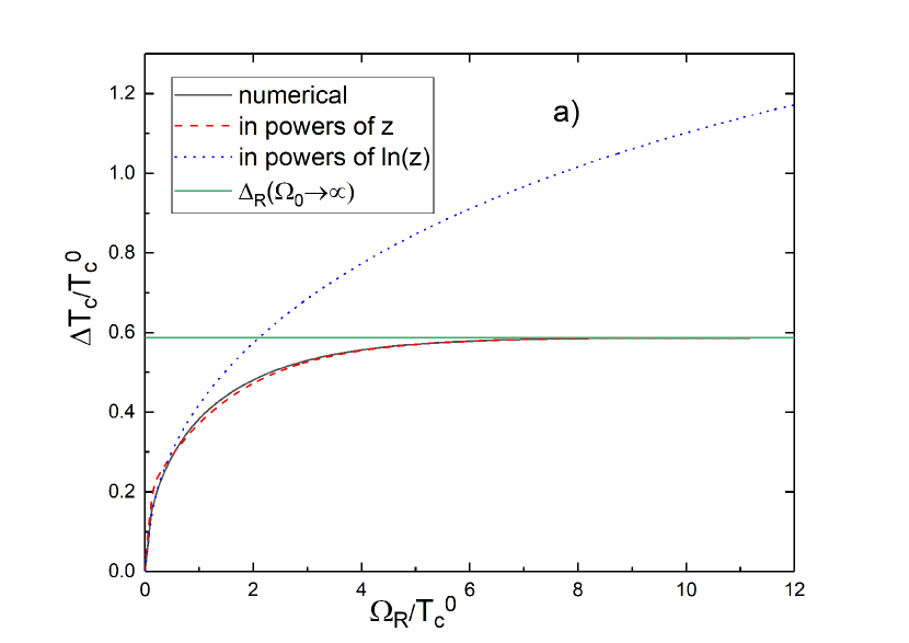
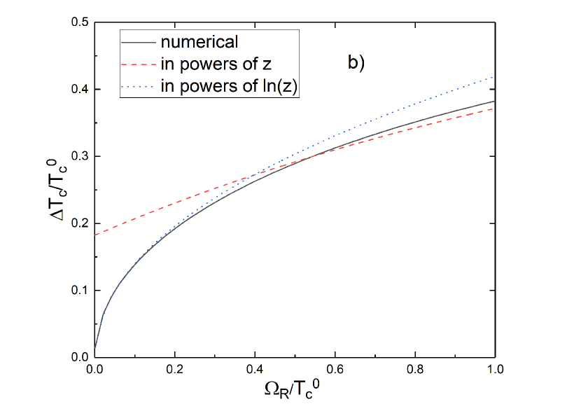
Figure 1: (a) The shift of critical temperature due to Rabi coupling vs the dimensionless parameter $\Omega_{R}/{T_{c}^{0}}$. The results of the exact solution of the Eq. (47), expansion in powers of $z=\exp(-\Omega_{R}/{T_{c}^{0}})$, (53) and in powers of $\ln(z)$, (52) are presented by solid, dashed and dotted curves , respectively. (b) The same as in (a) but in a rather larger scale for $\Omega_{R}/{T_{c}^{0}}\leq 1$

As it is seen from Figs.1 the shift is always positive and tends to a plateau at large $\Omega_{R}$ for a finite ${T_{c}^{0}}$. This asymptotic value can be easily evaluated from the Eq. (47). In fact, since $z(\Omega_{R}\rightarrow\infty)=0$, and Li$(3/2,0)=0$ one obtains $\Delta_{R}(\Omega_{R}\rightarrow\infty)=2^{2/3}-1\approx 0.5874$. The dashed and dotted curves in Figs. 1 are approximative solutions of Eq. (47), while the solid one is the exact numerical solution.

In the literature one can find two kinds of approximations for Li$(3/2,z)$ (see e.g. [41]):

$$\small\begin{array}[]{l}\text{Li}(3/2,z)=z+\displaystyle\frac{\sqrt{2}z^{2}}{4}+\displaystyle\frac{\sqrt{3}z^{3}}{9}+O(z^{4})\end{array}$$ (50)

and

$$\small\begin{array}[]{l}\text{Li}(3/2,z)=-2\sqrt{\pi}\sqrt{\ln(1/z)}+\zeta(3/2)+\\ \zeta(1/2)\ln(z)+\displaystyle\frac{\zeta(-1/2)}{2}\ln^{2}(z)+O(\ln^{3}(z))\end{array}$$ (51)

The former (50) is good for small $z<0.3$ ( that is for large $\Omega_{R}$) and the latter (51) for rather large $0.3\leq z\leq 1$ ( for small $\Omega_{R}$). Thus using these expansions in (47) and solving the equation iteratively we find following approximations

$$\small\begin{array}[]{l}\Delta_{R}(\Omega_{R}/{T_{c}^{0}}\leq 1)=\displaystyle\frac{432^{1/3}\sqrt{\pi}2^{2/3}}{18\zeta(3/2)}\sqrt{x}+\displaystyle\frac{\pi+\zeta(1/2)\zeta(3/2)}{3(\zeta(3/2))^{2}}x+O(x^{3/2})\approx 0.45\sqrt{x}-0.033x\end{array}$$ (52)

for small and

$$\small\begin{array}[]{l}\Delta_{R}(\Omega_{R}/{T_{c}^{0}}>>1)\approx-\displaystyle\frac{2^{5/2}\exp(-\frac{x}{2^{2/3}})}{3\zeta(3/2)}+2^{2/3}-1\approx 0.5874-0.4\exp({-{0.63x}})\end{array}$$ (53)

large values of the dimensionless parameter $x\equiv\Omega_{R}/{T_{c}^{0}}$. This is illustrated in Fig.1b, where dashed and dotted curves are appropriate for the Eqs. (53) and (52) respectively.

Note that, existing experiments are performed with $\Omega_{R}\sim 1000Hz\approx 0.48\cdot 10^{-7}$K at temperatures $T\sim 2\cdot 10^{-7}$ K , which corresponds to rather small values of ${\Omega_{R}}/{T_{c}^{0}}\sim 0.25$. From Fig.1b we conclude that, in reality one may use the approximation given by Eq. (52) which gives about $20\%$ near this region for the shift of the critical temperature due to Rabi coupling.

VI Conclusion

In present work we have studied Rabi coupled binary Bose system within the Gaussian (bilinear) approximation in the framework of the mean field theory. We have shown that for this system at finite temperatures BEC can exist only for a symmetric case ( $g_{a}=g_{b}$) with an equal population, otherwise only a crossover transition may take place. For the first time we have derived Hugenholtz - Pines relations and an equation for the shift of the critical temperature in the presence of one body interaction. Although our extended HP relations: $\Sigma_{n}-\Sigma_{an}=\mu+\Omega_{R}/2$, and $\Sigma_{n}^{ab}=\Sigma_{an}^{ab}$ are proved within the field theoretical Gaussian approximation, we expect that they will remain true beyond this approximation also and can be proved more accurately, say in the spirit of works [32, 30]

As to the critical temperature $T_{c}$ of a BEC transition in Rabi coupled two component system, it has never been studied before. So, we obtained rather simple equation to determine $T_{c}$ as well as its shift due to Rabi coupling. The solutions of this equation may be apparently presented analytically for small (or large) values of the input parameter $\Omega_{R}/{T_{c}^{0}}$. The shift, as we predicted, is positive and should be about $\sim 20\%$ in existing experimental measurements with the moderate value of parameter $\Omega_{R}/{T_{c}^{0}}\sim 0.2$. Principally, one may assume possibility of making measurements with rather large values of $\Omega_{R}/{T_{c}^{0}}$ also. For such experiments, we predict that the shift should go to its asymptotic value $\Delta T_{c}/{T_{c}^{0}}\leq 2^{2/3}-1\approx 0.58$ , displaying a plateau. We hope that, this prediction can be verified in future experiments performed at finite temperatures. On the other hand it would be also interesting to estimate the shift by using quite other approximations with a different perturbation scheme, for example, used in Refs. [15, 16].

Moreover, we have proved that, physical observables , particularly $\Delta T_{c}/{T_{c}^{0}}$ do not depend on the sign of one body interaction i.e. on the phase of Rabi coupling $\omega_{R}$. Possible effect of changing the sign of this interaction could be reflected only in the relative phase of the two condensates $\xi$ under the condition $\xi\omega_{R}=-1$.

Note that, other problems concerning these systems, such as the temperature dependence of thermodynamic parameters, as well as stability conditions [12] are left beyond the scope of the present work. We shall study these problems in our forthcoming paper, where we use a more accurate approximation than the Gaussian one and make an attempt to extend the equation (24) for a general asymmetric binary Bose system with a crossover [24].

Appendix A Relation between the phases and phase invariance

In present Appendix we show that, the stability condition with respect to the relative phase $\xi=\exp(i\theta)$ leads to the relation $\xi\omega_{R}=-1$. In fact, the relative phase angle $\theta$, should correspond to the minimum of $\Omega_{0}$:

$$\small\frac{\partial\Omega_{0}}{\partial\theta}=0,\quad\frac{\partial^{2}\Omega_{0}}{\partial\theta^{2}}>0$$ (A.1)

In general, $\Omega_{0}$ is given by

$$\small\begin{array}[]{l}\Omega_{0}=V[-\mu\rho_{0a}-\mu\rho_{0b}+\displaystyle\frac{g_{a}\rho_{0a}^{2}}{2}+\displaystyle\frac{g_{b}\rho_{0b}^{2}}{2}+g_{ab}\rho_{0a}\rho_{0b}+\displaystyle\frac{\Omega_{R}\sqrt{\rho_{0a}\rho_{0b}}\xi(\omega_{R}+\omega_{R}^{\star})}{2}]\end{array}$$ (A.2)

Besides, in stable equilibrium, the variational parameters $\rho_{0a}$ and $\rho_{0b}$ should satisfy the saddle-point equations [12, 27, 28]

$$\frac{\partial\Omega_{0}}{\partial\rho_{0a}}=0,\quad\frac{\partial\Omega_{0}}{\partial\rho_{0b}}=0\quad$$

$$\left(\frac{\partial^{2}\Omega_{0}}{\partial\rho_{0a}^{2}}\right)\left(\frac{\partial^{2}\Omega_{0}}{\partial\rho_{0b}^{2}}\right)-\left(\frac{\partial^{2}\Omega_{0}}{\partial\rho_{0a}\partial\rho_{0b}}\right)>0$$ (A.3)

Now bearing in mind $\omega_{R}=e^{-i\theta_{R}}$, and using Eqs. (A.1), (A.2), we obtain

$$\small\begin{split}\frac{\partial\Omega_{0}}{\partial\theta}=-V\Omega_{R}\sqrt{\rho_{0a}\rho_{0b}}\sin(\theta-\theta_{R})=0\\ \frac{\partial^{2}\Omega_{0}}{\partial\theta^{2}}=-V\Omega_{R}\sqrt{\rho_{0a}\rho_{0b}}\cos(\theta-\theta_{R})>0\end{split}$$ (A.4)

which lead to the well known [1, 9, 10] result: $\theta-\theta_{R}=\pi(2n+1)$ i.e. $\omega_{R}\xi=-1$. This physically means that, when the system goes into its equilibrium state, it will choose the relative phase between the two condensates by itself, preferring the case with $\xi=-\omega_{R}$, where $\omega_{R}$ is in fact the sign of the one body interaction. For example, if the latter is negative, $\omega_{R}=-1$ , then the condensates will coexist with the same phase $\xi=+1$, and vise versa. Moreover, particularly , in both cases, with $\xi=\pm 1$ there always exist in phase and out of phase excitations. The former correspond to the density branch $\omega_{d}$, while the latter to the spin branch $\omega_{s}$ , as it has been clarified in Refs. [39, 42]

Below we show that physical observables do not depend on the relative phase $\xi$. Actually, in the symmetric case for the self energies we have

$$\small\begin{split}&X_{1}=X_{3}=-\mu+3\rho_{0a}g+\rho_{0a}g_{ab}=\Sigma_{n}+\Sigma_{an}-\mu\\ &X_{2}=X_{4}=-\mu+\rho_{0a}g+\rho_{0a}g_{ab}=\Sigma_{n}-\Sigma_{an}-\mu\\ &X_{5}=2\xi g_{ab}\rho_{0a}+\frac{\Omega_{R}\omega_{R}}{2},\quad X_{6}=\frac{\Omega_{R}\omega_{R}}{2}\end{split}$$ (A.5)

and for the dispersions:

$$\small\begin{array}[]{l}\omega_{1}=\sqrt{(\varepsilon_{k}+X_{2}+X_{6})(\varepsilon_{k}+X_{1}+X_{5})}\\ \omega_{2}=\sqrt{(\varepsilon_{k}+X_{2}-X_{6})(\varepsilon_{k}+X_{1}-X_{5})}\end{array}$$ (A.6)

Now from Eqs. (33), (A.5) and (A.6) it is seen that e.g. $\rho_{1a}$ is phase invariant, that is $\rho_{1a}(\xi,\omega_{R})=\rho_{1a}(-\xi,-\omega_{R})$, since the transformation $(\xi,\omega_{R})\leftrightarrow(-\xi,-\omega_{R})$ is equivalent to the following replacements: $X_{5}\leftrightarrow-X_{5}$, $X_{6}\leftrightarrow-X_{6}$, $\omega_{1}\leftrightarrow\omega_{2}$. Note that, this statement holds true both for the condensed as well as normal states. Phase invariance of other observables can be proven in the same way.

References

• [1] L. Pitaevskii and S. Stringari, Bose-Einstein Condensation and Superfluidity (Oxford University Press, New York, 2015)
• [2] D. S. Hall, M. R. Matthews, J. R. Ensher, C. E. Wieman, and E. A. Cornell, Dynamics of Component Separation in a Binary Mixture of Bose-Einstein Condensates, Phys. Rev. Lett. 81, 1539 (1998).
• [3] M. R. Matthews, B. P. Anderson, P. C. Haljan, D. S. Hall, M. J. Holland, J. E. Williams, C. E. Wieman, and E. A. Cornell, Watching a Superfluid Untwist Itself: Recurrence of Rabi Oscillations in a Bose-Einstein Condensate, Phys. Rev.Lett. 83, 17, (1999).
• [4] T. Zibold, E. Nicklas, Ch. Gross, and M. K. Oberthaler, Classical Bifurcation at the Transition from Rabi to Josephson Dynamics, Phys. Rev. Lett. 105, 204101 , (2010).
• [5] L. Lavoine, A. Hammond, A. Recati, D.S. Petrov, and T. Bourdel, Beyond-mean-field effects in Rabi-coupled two-component Bose-Einstein condensate, Phys. Rev. Lett. 127, 203402, (2021).
• [6] J. Williams, R. Walser, J. Cooper, E. A. Cornell, and M. Holland, Excitation of a dipole topological state in a strongly coupled two-component Bose-Einstein condensate, Phys. Rev. A 61, 033612, (2000).
• [7] A. Niederberger, T. Schulte, J. Wehr, M. Lewenstein, L. Sanchez-Palencia, and K. Sacha, Disorder-Induced Order in Two-Component Bose-Einstein Condensates, Phys. Rev. Lett. 100, 030403 (2008).
• [8] Xiao Yin and Leo Radzihovsky , Quench dynamics of a strongly interacting resonant Bose gas, Phys. Rev. A 88, 063611 (2013)
• [9] S. Lellouch, Tung-Lam Dao, T. Koffel, and L. Sanchez-Palencia, Two-component Bose gases with one-body and two-body couplings, Phys. Rev. A 88, 063646 (2013).
• [10] M. Abad and A. Recati, A study of coherently coupled two-component Bose-Einstein condensates, Eur. Phys. J. D 67 (7), 148 (2013).
• [11] A. Aftalion and P. Mason, Rabi-coupled two-component Bose-Einstein condensates: Classification of the ground states, defects, and energy estimates, Phys. Rev. A 94, 023616 (2016).
• [12] A. Cappellaro, T. Macri, G. F. Bertacco and L. Salasnich, Equation of state and self-bound droplet in Rabi-coupled Bose mixtures, Sci Rep 7, 13358 (2017).
• [13] M. Kobayashi, M. Eto, M. Nitta, Berezinskii-Kosterlitz-Thouless Transition of Two-component Bose Mixtures with Intercomponent Josephson Coupling, Phys. Rev. Lett. 123, 075303 (2019).
• [14] V. I. Yukalov and E. P. Yukalova, Bose - Einstein condensation temperature of weakly interacting atoms, Laser Phys. Lett. 14, 073001 (2017).
• [15] G. Baym, J. -P. Blaizot, M. Holzmann, F. Laloe, and D. Vautherin, The Transition Temperature of the Dilute Interacting Bose Gas, Phys. Rev. Lett. 83, 1703 (1999).
• [16] B. Kastening, Bose-Einstein condensation temperature of a homogenous weakly interacting Bose gas in variational perturbation theory through seven loops, Phys. Rev. A 69, 043613 (2004).
• [17] Frederico F. de Souza Cruz and Marcus B. Pinto, Transition temperature for weakly interacting homogeneous Bose gases, Phys. Rev. B, 64, 014515 (2001).
• [18] V. I. Yukalov, A. Rakhimov and S. Mardonov, Quasi-equilibrium mixture of itinerant and localized bose atoms in optical lattice, Laser Phys. 21, 264-270 (2011).
• [19] H. Kleinert, Z. Narzikulov and A. Rakhimov, Phase transitions in three-dimensional bosonic systems in optical lattices, J. Stat. Mech. P01003, 1742 - 5468 (2014).
• [20] A. Rakhimov and I. N. Askerzade, Critical temperature of noninteracting bosonic gases in cubic optical lattices at arbitrary integer fillings, Phys. Rev. E 90, 032124 (2014).
• [21] A. Rakhimov and I. N. Askerzade, Thermodynamics of noninteracting bosonic gases in cubic optical lattices versus ideal homogeneous Bose gases, Int. J. Mod. Phys. B 29, 1550123 (2015).
• [22] A. Rakhimov, Sh. Mardonov, E. Ya. Sherman and A. Schilling, The effects of disorder in dimerized quantum magnets in mean field approximations, New J. Phys. 14, 113010 (2012).
• [23] A.V. Lopatin and V. M. Vinokur, Thermodynamics of the Superfluid Dilute Bose Gas with Disorder, Phys. Rev. Lett. 88, 235503 (2002).
• [24] A. Khudoyberdiev, A. Rakhimov, and A. Schilling, Bose-Einstein condensation of triplons with a weakly broken U(1) symmetry, New J. Phys. 19, 113002 (2017).
• [25] A. Rakhimov, A. Khudoyberdiev, L. Rani, and B. Tanatar, Spin-gapped magnets with weak anisotropies I: Constraints on the phase of the condensate wave function, Ann. Phys. 424, 168361 (2021).
• [26] A. Rakhimov, A. Khudoyberdiev, and B. Tanatar, Effects of exchange and weak Dzyaloshinsky- Moriya anisotropies on thermodynamic characteristics of spin-gapped magnets, Int. J. Mod. Phys. B 35, 2150223 (2019).
• [27] T. Haugset, H. Haugerud and F. Ravndal, Thermodynamics of a weakly interacting Bose - Einstein gas, Ann. Phys. (N.Y.) 266 , 27 (1998)
• [28] J. O. Andersen, Theory of the weakly interacting Bose gas, Rev. Mod. Phys. 76, 599 (2004).
• [29] N. M. Hugenholtz and D. Pines, Ground-State Energy and Excitation Spectrum of a System of Interacting Bosons, Phys. Rev. 116, 489 (1959).
• [30] N. N. Bogolubov, Lectures on Quantum Statistics, vol. 2, Gordon and Breach, New York, (1970).
• [31] Yu. A. Nepomnyashchil, The microscopic theory of a mixture of superfluid liquids, Zh. Eksp. Teor. Fiz. 70, 1071O80 (1976).
• [32] Shohei Watabe, Hugenholtz-Pines theorem for multicomponent Bose-Einstein condensates, Phys. Rev. A 103, 053307 (2021).
• [33] Henk T.C. Stoof, Koos B. Gubbels, Dennis B.M. Dickerscheid, Ultracold Quantum Fields, Theoretical and Mathematical Physics, Springer (2004).
• [34] A. Rakhimov, Tan’s contact as an indicator of completeness and self-consistency of a theory, Phys. Rev. A 102, 063306 (2020).
• [35] A. Rakhimov, T. Abdurakhmonov and B. Tanatar, Critical behavior of Tan’s contact for bosonic systems with a fixed chemical potential, J. Phys.: Condens. Matter 33, (2021)
• [36] V. I. Yukalov, Theory of cold atoms: Bose - Einstein statistics, Laser Phys. 26, 062001 (2016)
• [37] P.C. Hohenberg and P.C. Martin Microscopic theory of superfluid helium, Ann. Phys. 34, 291 (1965).
• [38] A. Rakhimov, and Z. Narzikulov, Hohenberg-Martin Dilemma for Bose Condensed Systems and its Solution, Complex Phenomena in Nanoscale Systems. NATO Science for Peace and Security Series B: Physics and Biophysics. Springer, Dordrecht (2009).
• [39] A. Rakhimov, T. Abdurakhmonov, Z. Narzikulov, and V. I. Yukalov, Self-consistent theory of a homogeneous binary Bose mixture with strong repulsive interspecies interaction, Phys. Rev. A 106, 033301 (2022)
• [40] V.I. Yukalov and H. Kleinert Gapless Hartree-Fock-Bogoliubov approximation for Bose gases, Phys. Rev. A, 73, 063612 (2006).
• [41] D. C. Wood, The computation of polylogarithm, Tech. Report Technical Report 15-92, Univer- sity of Kent (1992).
• [42] J. H. Kim, D. Hong, and Y. Shin, Observation of two sound modes in a binary superfluid gas, Phys. Rev. A 101, 061601(R) (2020).