Photometric Objects Around Cosmic Webs (PAC) Delineated in a Spectroscopic Survey. IV. High Precision Constraints on the Evolution of Stellar-Halo Mass Relation at Redshift $z<0.7$

Abstract

Taking advantage of the Photometric objects Around Cosmic webs (PAC) method developed in Paper I, we measure the excess surface density $\bar{n}_{2}w_{{\rm{p}}}$ of photometric objects around spectroscopic objects down to stellar mass $10^{8.0}M_{\odot}$, $10^{9.2}M_{\odot}$ and $10^{9.8}M_{\odot}$ in the redshift ranges of $z_{s}$$<0.2$, $0.2<z_{s}<0.4$ and $0.5<z_{s}<0.7$ respectively, using the data from the DESI Legacy Imaging Surveys and the spectroscopic samples of Slogan Digital Sky Survey (i.e. Main, LOWZ and CMASS samples). We model the measured $\bar{n}_{2}w_{{\rm{p}}}$ in N-body simulation using abundance matching method and constrain the stellar-halo mass relations (SHMR) in the three redshift ranges to percent level. With the accurate modeling, we demonstrate that the stellar mass scatter for given halo mass is nearly a constant, and that the empirical form of Behroozi et al describes the SHMR better than the double power law form at low mass. Our SHMR accurately captures the downsizing of massive galaxies since $z_{s}=0.7$, while it also indicates that small galaxies are still growing faster than their host halos. The galaxy stellar mass functions (GSMF) from our modeling are in perfect agreement with the model-independent measurements in Paper III, though the current work extends the GSMF to a much smaller stellar mass. Based on the GSMF and SHMR, we derive the stellar mass completeness and halo occupation distributions for the LOWZ and CMASS samples, which are useful for correctly interpreting their cosmological measurements such as galaxy-galaxy lensing and redshift space distortion.

1 Introduction

With the rapid development of cosmology, we have entered an era of understanding galaxy formation in the cosmological framework (Mo et al., 2010; Frenk & White, 2012; Somerville & Davé, 2015; Naab & Ostriker, 2017). In this framework, galaxies reside in the dark matter halos, and the growth of galaxies is closely related to the growth of their host halos. Thus, precise measurement of the galaxy-halo connection is one of the most important issues in galaxy formation (Wechsler & Tinker, 2018). Moreover, accurate constraints on the the galaxy-halo connection can in turn benefit the cosmology studies, such as galaxy-galaxy gravitational lensing (Bartelmann & Schneider, 2001; Treu, 2010) and redshift space distortion of galaxy distribution (Kaiser, 1987; Scoccimarro, 2004), by connecting the observations of galaxies to the theories of dark matter halos.

The stellar-halo mass relation (SHMR) is one of the most commonly used relations to populate galaxies to halos, in which larger halos host more massive galaxies with a relatively tight scatter. Various methods have been used to model the SHMR at different redshifts, including abundance matching (AM, Guo et al., 2010; Wang & Jing, 2010), conditional luminosity function (CLF, Yang et al., 2012) and empirical modeling (EM, Moster et al., 2013, 2018; Behroozi et al., 2013, 2019). No matter how the methods were implemented, they all rely on the measurements of observables such as the galaxy stellar mass function (GSMF) and galaxy clustering (GC). Although relatively tight constraints have achieved at the high mass end of the SHMR for local $z_{s}\approx 0$, the results at the low mass end still vary widely between studies (e.g. Guo et al., 2010; Yang et al., 2012; Moster et al., 2013; Behroozi et al., 2019) , due to the lack of accurate measurements of GSMF and GC at the faint end. At higher redshift, the measurement of SHMR is more difficult and more uncertain since there does not exist a large stellar-mass limited redshift sample.

Measurements of GSMF and GC rely on accurate redshift information. In the past two decades, there has been significant progress in spectroscopic surveys (York et al., 2000; Colless et al., 2001; Steidel et al., 2003; Le Fèvre et al., 2005; Ahn et al., 2012; Bolton et al., 2012; Garilli et al., 2014; Takada et al., 2014; DESI Collaboration et al., 2016; Ahumada et al., 2020). In the local universe ($z_{s}\sim 0$), the measurements of GSMF and GC are mainly from the large spectroscopic surveys, in particular the Sloan Digital Sky Survey (SDSS, York et al., 2000) and the Two Degree Field Galaxy spectroscopic survey (2dFGRS, Colless et al., 2001)), down to $10^{9.0}M_{\odot}$ (Cole et al., 2001; Norberg et al., 2002; Li et al., 2006; Baldry et al., 2008; Li & White, 2009). However, for the faint galaxies, the accuracy of the measurements, especially the GC, is still very limited by the survey volume. At intermediate redshifts ($z_{s}<1.0$), deeper spectroscopic surveys begin to dominate the measurements. The DEEP2 Galaxy spectroscopic survey (Davis et al., 2003), the VIMOS-VLT Deep Survey (VVDS, Le Fèvre et al., 2005) and the VIMOS Public Extragalactic spectroscopic survey (VIPERS, Garilli et al., 2014) have been used to successfully measure GC and GSMF for galaxies down to $10^{10.0}M_{\odot}$ (Pozzetti et al., 2007; Meneux et al., 2008; Mostek et al., 2013; Marulli et al., 2013; Davidzon et al., 2013), though the measurements are limited by the survey volumes at the high stellar mass end (i.e. $>10^{11.0}M_{\odot}$). Similarly, measuring GC and GSMF at the faint end (i.e. $<10^{10.0}M_{\odot}$) is also very challenging at $z_{s}\sim 0.5$ for the magnitude-limited redshift surveys.

Many attempts have been made to push the measurement of GSMF to higher redshifts ($z_{s}>1.0$) using deep multi-band photometric surveys (Fontana et al., 2006; Ilbert et al., 2013; Muzzin et al., 2013; Tomczak et al., 2014; Mortlock et al., 2015; Davidzon et al., 2017; Wright et al., 2018; Leja et al., 2020; McLeod et al., 2021; Shuntov et al., 2022), which are usually deeper and more complete in terms of the stellar mass. However, the deep multi-band photometric surveys usually have very small survey area ($1\sim 2\ \rm{deg}^{2}$), since they require long exposure time to reach very faint sources and multiple bands from UV to IR to obtain relatively accurate photometric redshifts (photoz) for faint objects. Thus, the cosmic variance could be significant, especially for massive galaxies. In addition, although faint sources are detected in the deep photometric surveys, the photometric redshifts derived for them are usually trained with the the spectroscopic data, which may not be complete for all type of faint sources, and therefore lead to larger photoz errors. These effects may all introduce uncertainties in the measurements of GSMF and GC.

Systematic bias between the measurements in different surveys can also affect the study of SHMR. Many studies (Yang et al., 2012; Moster et al., 2013, 2018; Behroozi et al., 2013, 2019) collected the GSMF measurements from different surveys at different redshifts to model the evolution of SHMR. However, as shown in Xu et al. (2022a), the systematic bias of GSMF is still very large ($\sim 30\%$) between different studies at the high mass end even after careful calibration, which may significantly influence the results of SHMR.

In Xu et al. (2022b, hearafter Paper I), on the basis of Wang et al. (2011), we developed a method named Photometric objects Around Cosmic webs (PAC) to estimate the excess surface density $\bar{n}_{2}w_{{\rm{p}}}$ of photometric objects with certain physical properties around spectroscopically identified sources, which can take full use of the spectroscopic and deeper photometric surveys. With PAC, we can measure $\bar{n}_{2}w_{{\rm{p}}}$ for galaxies to a much lower stellar mass than one can with the spectroscopic survey only. Another advantage is that $\bar{n}_{2}w_{{\rm{p}}}$ is measured in a uniform way at different redshifts, since the same photometric catalog and the same analysis method (i.e stellar mass measurement method) are used. Obviously the quantity contains the desired information of both GSMF and GC.

In this paper, we will measure $\bar{n}_{2}w_{{\rm{p}}}$ at different redshifts with Dark Energy Camera Legacy Survey (DECaLS) photometric catalogs and Slogan Digital Sky Survey (SDSS) Main, LOWZ and CMASS spectroscopic samples. Then, we will model the PAC measurements using the abundance matching method and constrain the evolution of the SHMR. We will compare the derived GSMF with the model independent measurements from Xu et al. (2022a, hearafter Paper III) to test the reliability of the results, and we will show how much we can extend GSMF to a small stellar mass in this study. Based on our SHMR and GSMF, we will also derive the stellar mass completeness and halo occupation distributions (HOD, Jing et al., 1998; Peacock & Smith, 2000; Ma & Fry, 2000; Seljak, 2000; Berlind & Weinberg, 2002; Yang et al., 2003; Zheng et al., 2005; Zu & Mandelbaum, 2015) for the LOWZ and CMASS samples, which can be useful for cosmological interpretation of their clustering and lensing measurements.

We introduce the PAC method and show the measurements in Section 2. In Section 3, we model the measurements in N-body simulation and give the SHMR. In Section 4, we derive the HODs of spectroscopic samples. We briefly summarize our results in Section 5. We adopt the cosmology with $\Omega_{m}=0.268$, $\Omega_{\Lambda}=0.732$ and $H_{0}=71{\rm\ km/s/Mpc}$ throughout the paper.

2 observation and measurements

In this section, we first give a brief summary about the Photometric objects Around Cosmic webs (PAC) method and the spectroscopic and photometric samples used in this work. Then we investigate the stellar mass completeness of the samples and present the final PAC measurements.

2.1 Photometric objects Around Cosmic webs (PAC)

Supposing we want to study two populations of galaxies, with one (${\rm{pop}}_{1}$) from a spectroscopic catalog and the other (${\rm{pop}}_{2}$) from a photometric catalog, within a relatively narrow redshift range. We proposed a method called PAC in Paper I that can accurately measure the excess surface density $\bar{n}_{2}w_{\rm{p}}(r_{\rm{p}})$ of ${\rm{pop}}_{2}$ around ${\rm{pop}}_{1}$ with certain physical properties:

$$\bar{n}_{2}w_{\rm{p}}(r_{\rm{p}})=\frac{\bar{S}_{2}}{r_{1}^{2}}w_{12,\rm{weight}}(\theta)\,\,,$$ (1)

where $\bar{n}_{2}$ and $\bar{S}_{2}$ are the mean number density and mean angular surface density of $\rm{pop}_{2}$, $r_{1}$ is the comoving distance to $\rm{pop}_{1}$, and $w_{\rm{p}}(r_{\rm{p}})$ and $w_{12,\rm{weight}}(\theta)$ are the projected cross-correlation function (PCCF) and the weighted angular cross-correlation function (ACCF) between $\rm{pop}_{1}$ and $\rm{pop}_{2}$ with $r_{\rm{p}}=r_{1}\theta$. Since $\rm{pop}_{1}$ has a redshift distribution, $w_{12}(\theta)$ is weighted by $1/r^{2}_{1}$ to account for the effect that, at fixed $\theta$, $r_{\rm{p}}$ varies with $r_{1}$. Using PAC, we can measure the rest-frame physical properties of $\rm{pop}_{2}$ statistically without the need of the redshift information of $\rm{pop}_{2}$, for which we can take full use of the deep photometric surveys. The following are the main steps of PAC:

1. Split $\rm{pop}_{1}$ into narrower redshift bins, mainly accounting for the fast change of $r_{1}$ with redshift.

2. Assuming all galaxies in $\rm{pop}_{2}$ have the same redshift as the mean redshift of each redshift bin, calculate the physical properties of $\rm{pop}_{2}$ using methods such as spectral energy distribution (SED). Therefore, in each redshift bin of $\rm{pop}_{1}$, there is a physical property catalog of $\rm{pop}_{2}$ .

3. In each redshift bin, select $\rm{pop}_{2}$ with certain physical properties and calculate $\bar{n}_{2}w_{\rm{p}}(r_{\rm{p}})$ according to Equation 1. The foreground and background objects with wrong properties are cancelled out through ACCF and only $\rm{pop}_{2}$ around $\rm{pop}_{1}$ with correct redshifts left.

4. Combine the results from different redshift bins by averaging with proper weights.

For more details, we refer to Paper I.

Table 1: Final designs for the PAC measurements.

redshift	Survey	$\rm{pop}_{1}$a	$\rm{pop}_{2}$b	PAC redshift bins
		($M_{\odot}$)	($M_{\odot}$)
$[0.05,0.2]$	Main	$[10^{10.3},10^{11.3}]$	$[10^{7.9},10^{11.7}]$	$[0.05,0.075],[0.075,0.1],[0.1,0.15],[0.15,0.2]$
$[0.2,0.4]$	LOWZ	$[10^{11.3},10^{11.9}]$	$[10^{9.1},10^{11.9}]$	$[0.2,0.3],[0.3,0.4]$
$[0.5,0.7]$	CMASS	$[10^{11.3},10^{11.9}]$	$[10^{9.7},10^{11.9}]$	$[0.5,0.6],[0.6,0.7]$

• Stellar mass ranges of $\rm{pop}_{1}$ with an fiducial equal logarithmic bin width of $10^{0.2}M_{\odot}$.

• Stellar mass ranges of $\rm{pop}_{2}$ with an fiducial equal logarithmic bin width of $10^{0.2}M_{\odot}$.

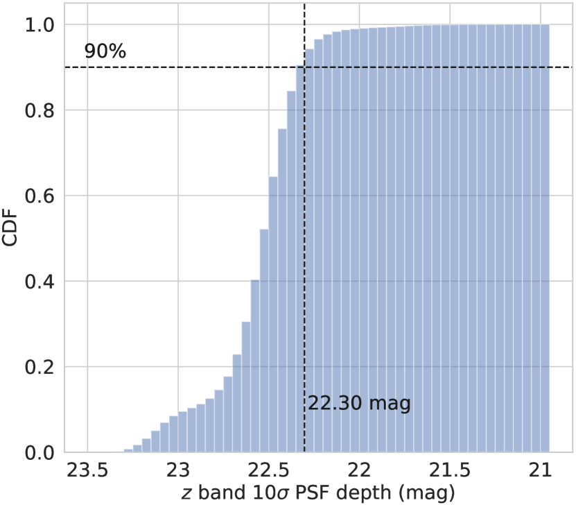
Figure 1: Cumulative distribution functions of the $r$ (left) and $z$ (right) band $10\sigma$ point source depths for DECaLS.

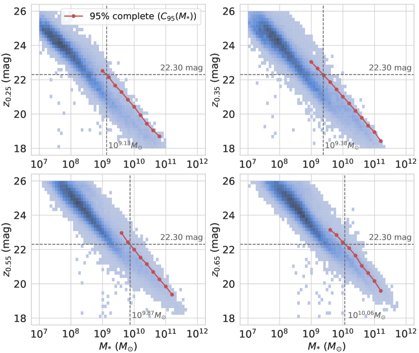
Figure 2: Stellar mass - $z$ band magnitude relations for DES Deep Field galaxies in redshift ranges of $[0.2,0.3]$, $[0.3,0.4]$, $[0.5,0.6]$ and $[0.6,0.7]$. Red lines with dots show the $95\%$ completeness limits $C_{95}(M_{*})$ varying with the stellar mass at each redshifts. Grey dashed lines show the stellar mass limits for DECLaS with the $z$ band depth of $22.30\ \rm{mag}$.

Figure 3: PAC measurements and fittings from the BP13 model for the Main sample redshift range ($z_{s}<0.2$) according to the designs in Table 1. Dots with error bars show the measurements and lines with shadows are the best-fit results and $1\sigma$ errors from AM modelings. We only show the results of 3 ${\rm{pop}}_{1}$ mass bins ($10^{10.4},10^{10.8},10^{11.2}M_{\odot}$) out of the total 5 for better illustration, and the results of the last ${\rm{pop}}_{2}$ bins ($10^{11.6}M_{\odot}$) are multiplied by $10$.

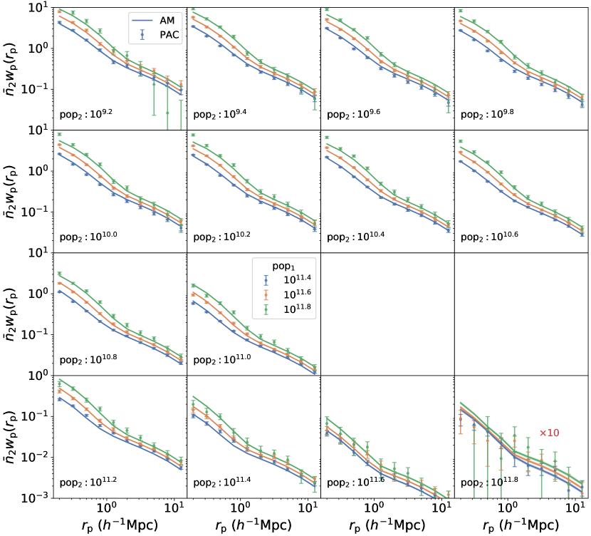
Figure 4: The same as Figure 3 but for the LOWZ redshift range ($0.2<z_{s}<0.4$).

Figure 5: The same as Figure 3 but for the CMASS redshift range ($0.5<z_{s}<0.7$).

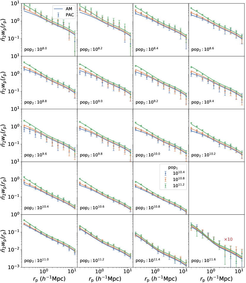
Figure 6: The same as Figure 3 but for the Main sample redshift range ($z_{s}<0.2$) with fittings from the DP model.

2.2 Spectroscopic and photometric samples

In this work, we use the same spectroscopic and photometric data as used in Paper III. We summary their key features in the following.

For photometric data, we use photometric catalog of DECaLS from the DR9 of the DESI Legacy Imaging Survey (Dey et al., 2019). It observes around $9000\ {\rm{deg}}^{2}$ in both the Northern and Southern Galactic caps (NGC and SGC) at $\rm{Dec}\leq 32\ \rm{deg}$ in $g$, $r$ and $z$ bands with median $5\sigma$ point source depths of $24.9$, $24.2$ and $23.3$ respectively. DECaLS also includes the data from the deeper Dark Energy Survey (DES; Dark Energy Survey Collaboration et al. 2016) covering additional $5000\ {\rm{deg}}^{2}$ in the SGC. The images are processed using Tractor (Lang et al., 2016) to perform source extraction. The sources are then modeled with parametric profiles convolved with a specific point spread function (PSF), including a delta function for the point source, exponential law, de Vaucouleurs law, and a Sérsic profile. We use their best-fit model magnitudes throughout the paper. We only use the footprints that have been observed at least once in all three bands, and perform bright star mask and bad pixel mask to the catalog using the MASKBITS provided by the Legacy Surveys. Additional masks are used to match the geometry of the spectroscopic sample in each redshift. Galactic extinction is corrected for all the sources using the maps of Schlegel et al. (1998). To reject stars, we exclude sources with point source (PSF) morphologies, and we adopt color cuts in $r-z$ vs. $z-W1$ diagram calibrated in Paper III (see Figure 1) to further remove stellar objects, with $W1$ band data from the Wide-field Infrared Survey Explorer (WISE) (Wright et al., 2010). The stars have

$$(z-W1<0.8\times(r-z)-1.0)\ {\rm{AND}}\ (r-z>1.0)\,\,.$$ (2)

For spectroscopic data, all the catalogs used in this work are from SDSS (York et al., 2000)). We use the SDSS DR7 Main sample (Abazajian et al., 2009), SDSS-III BOSS DR12 LOWZ and CMASS samples (Alam et al., 2015; Reid et al., 2016) for three redshift ranges $z_{s}<0.2$, $0.2<z_{s}<0.4$ and $0.5<z_{s}<0.7$ respectively. All the three samples are selected with $\rm{Dec}\leq 32\ \rm{deg}$ to match the footprint of DECaLS, and for the Main sample, only the NGC part is used since the SGC part is very small ($532\ {\rm{deg}}^{2}$). The spectroscopic sources are cross-matched with DECaLS to get the $g$, $r$ and $z$ band flux measurements.

2.3 Completeness and Designs

Based on the test in Paper I see Figure 3 there, we split LOWZ and CMASS samples into 2 and Main sample into 4 narrower redshift bins as listed in Table 1. According to the stellar mass distributions (Paper III Figure 2), we choose the stellar mass range of $\rm{pop}_{1}$ as $[10^{10.3},10^{11.3}]M_{\odot}$ for the Main sample and $[10^{11.3},10^{11.9}]M_{\odot}$ for LOWZ and CMASS, and we further split them into several stellar mass bins with an equal logarithmic interval of $0.2$.

As in Paper I and Paper III, we use the $r$ (for $z_{s}<0.2$) and $z$ (for $0.2<z_{s}<0.4$ and $0.5<z_{s}<0.7$) band $10\sigma$ point source depths of DECaLS to study the mass completeness of $\rm{pop}_{2}$. As shown in Figure 1, $90\%$ of the regions in DECaLS are deeper than $23.15$ mag and $22.30$ mag in $r$ band and $z$ band respectively. Thus, we use $r=23.15$ and $z=22.30$ as the galaxy depths for DECaLS.

In Paper III (see Figure 3), using the Galaxy And Mass Assembly (GAMA) DR4 spectroscopic data (Driver et al., 2022), we find that for $r$ band galaxy depth of $23.15\ \rm{mag}$, the complete stellar masses are $10^{7.61}M_{\odot}$, $10^{7.89}M_{\odot}$, $10^{8.31}M_{\odot}$ and $10^{8.61}M_{\odot}$ at redshift $0.075$, $0.1$, $0.15$ and $0.2$. Therefore, we choose the stellar mass range of $\rm{pop}_{2}$ as $[10^{7.9},10^{11.7}]M_{\odot}$ for $z_{s}<0.2$ and $\bar{n}_{2}w_{\rm{p}}$ is only calculated at $z_{s}<0.1$ and $z_{s}<0.15$ for $M_{*}<10^{8.3}M_{\odot}$ and $M_{*}<10^{8.5}M_{\odot}$ (See Appendix A for a validation).

The stellar mass limits that DECaLS can reach at $0.2<z_{s}<0.4$ and $0.5<z_{s}<0.7$ with $z$ band depth of $22.30$ mag remain to be investigated. We use the DES Year 3 Deep Field catalogs (Hartley et al., 2022) with photometric redshifts to explore the mass completeness in these redshift ranges. DES Deep can reach a $10\sigma$ $z$ band $2\ arcsec$ source depth of $24.3$ mag, much deeper than DECaLS, and we use the regions with full 8-band $ugrizJHK_{s}$ coverage ($5.88\ {\rm{deg}}^{2}$) to get more reliable photoz measurements. We adopt the photoz computed using EAZY (Brammer et al., 2008) provided by DES and calculate their physical properties using the SED code CIGALE (Boquien et al., 2019) with only the $grz$ band fluxes to be consistent with DECaLS. We use the Bruzual & Charlot (2003) stellar population synthesis models with a Chabrier (2003) initial mass function and a delayed star formation history $\phi(t)\approx t\exp{-t/\tau}$. We adopt three metallicities $Z/Z_{\odot}=0.4,\ 1\ \rm{and}\ 2.5$, where $Z_{\odot}$ is the metallicity of the Sun. And we use the Calzetti et al. (2000) extinction law for dust reddening with $0<E(B-V)<0.5$. In Figure 2 we show the stellar mass - $z$ band magnitude distributions for four redshift ranges $[0.2,0.3]$, $[0.3,0.4]$, $[0.5,0.6]$ and $[0.6,0.7]$. Following Paper I, we calculate the $z$ band completeness $C_{95}(M_{*})$ that $95\%$ of the galaxies are brighter than $C_{95}(M_{*})$ in the $z$ band for a given stellar mass $M_{*}$ (red lines). For the DECaLS $z$ band galaxy depth of $22.30$ mag, the complete stellar mass are $10^{9.13}M_{\odot}$, $10^{9.38}M_{\odot}$, $10^{9.87}M_{\odot}$ and $10^{10.06}M_{\odot}$ for the four redshifts. Thus, we choose the stellar mass range of ${\rm{pop}}_{2}$ as $[10^{9.1},10^{11.9}]M_{\odot}$ and $[10^{9.7},10^{11.9}]M_{\odot}$ for the LOWZ and CMASS redshift ranges respectively, and only measurements at $z_{s}<0.3$ and $z_{s}<0.6$ are used for $M_{*}<10^{9.3}M_{\odot}$ and $M_{*}<10^{9.9}M_{\odot}$.

We also split ${\rm{pop}}_{2}$ into smaller mass bins with an equal logarithmic interval of 0.2 in $\log M_{*}$ at each redshifts. The final designs are summarised in Table 1.

2.4 Measurements

We adopt the similar method used in Paper III to combine the results at different sky regions and redshift bins and to estimate the covariance matrices.

Let $\mathcal{A}=\bar{n}_{2}w_{\rm{p}}(r_{\rm{p}})$ for better representation. Assuming $\mathcal{A}$ is measured for $N_{r}$ redshift bins and $N_{s}$ sky regions (e.g. DECaLS NGC and DECaLS SGC), we further split each region into $N_{\rm{sub}}$ sub-regions for error estimation using jackknife resampling. According to Equation 1, $\mathcal{A}_{i,j,k}$ can be calculated in $i$th redshift bin, $j$th sky region and $k$th jackknife sub-sample using the Landy–Szalay estimator (Landy & Szalay, 1993). We first combine the measurements at different sky regions using the region area $w_{s}$ as weight:

$$\mathcal{A}_{i,k}=\frac{\sum_{j=1}^{N_{\rm{s}}}\mathcal{A}_{i,j,k}w_{\rm{s},j}}{\sum_{j=1}^{N_{\rm{s}}}w_{\rm{s},j}}\,\,.$$ (3)

Then, we estimate the mean values and the covariance matrices of the mean values for each redshift bins from $N_{\rm{sub}}$ sub-samples:

$$\mathcal{A}_{i}=\sum_{k=1}^{N_{\rm{sub}}}\mathcal{A}_{i,k}/N_{\rm{sub}}\,\,,$$ (4)

$$C_{ab,i}=\frac{N_{\rm{sub}}-1}{N_{\rm{sub}}}\sum_{k=1}^{N_{\rm{sub}}}(\mathcal{A}_{i,k}(r_{\rm{p}}^{a})-\mathcal{A}_{i}(r_{\rm{p}}^{a}))$$ (5)

$$\times(\mathcal{A}_{i,k}(r_{\rm{p}}^{b})-\mathcal{A}_{i}(r_{\rm{p}}^{b}))\,\,,$$

where $a$ and $b$ denotes the $a$th and $b$th radial bins. Finally, results from different redshift bins are combined according to the covariance matrices. Let $w_{i}(r_{\rm{p}})=\sigma^{-1}_{i}(r_{\rm{p}})$, where $\sigma_{i}^{2}(r_{\rm{p}})$ is the diagonal component of $\mathbf{C}_{i}$,

$$\mathcal{A}=\frac{\sum_{i=1}^{N_{\rm{r}}}\mathcal{A}_{i}w_{i}^{2}}{\sum_{i=1}^{N_{\rm{r}}}w_{i}^{2}}\,\,,$$ (6)

$$C_{ab}=\frac{\sum_{i=1}^{N_{\rm{r}}}w_{i}^{2}(r_{\rm{p}}^{a})w_{i}^{2}(r_{\rm{p}}^{b})C_{ab,i}}{\sum_{i=1}^{N_{\rm{r}}}w_{i}^{2}(r_{\rm{p}}^{a})\sum_{i=1}^{N_{\rm{r}}}w_{i}^{2}(r_{\rm{p}}^{b})}$$ (7)

According to the designs in Table 1, we measure $\bar{n}_{2}w_{\rm{p}}(r_{\rm{p}})$ in the radial range of $0.1h^{-1}{\rm{Mpc}}<r_{{\rm{p}}}<15h^{-1}\rm{Mpc}$ with $N_{\rm{sub}}=100$ for the 3 redshift ranges. The measurements are extended to scales far beyond the virial radii of halos hosting pop₁ galaxies, and thus include information of both centrals and satellites. The results are shown as dots with error bars in Figure 3, 4 and 5 for the Main sample, LOWZ and CMASS respectively. The square roots of the diagonal components of the covariance matrices are shown as error bars. The measurements are overall good for all mass bins within the whole radial ranges.

3 Simulation and Modelings

In this section, we introduce the simulation and abundance matching method used in this work, and show the constraints on SHMR from our PAC measurements.

Table 2: Posterior PDFs of the parameters from MCMC for the SHMR models.

redshift	model	$\log_{10}(M_{0})$	$\alpha$	$\delta$	$\beta$	$\log_{10}(k)/\log_{10}(\epsilon)$	$\sigma$
		($\log_{10}(h^{-1}M_{\odot})$)				($\log_{10}(M_{\odot})$)/($\log_{10}(h)$)
$z_{s}<0.2$	BP13	$11.338^{+0.027}_{-0.028}$	$0.484^{+0.027}_{-0.025}$	$3.041^{+0.134}_{-0.128}$	$1.632^{+0.039}_{-0.041}$	$-1.545^{+0.017}_{-0.017}$	$0.237^{+0.008}_{-0.008}$
$0.2<z_{s}<0.4$	BP13	$11.359^{+0.024}_{-0.025}$	$0.623^{+0.032}_{-0.030}$	$3.248^{+0.131}_{-0.125}$	$1.702^{+0.050}_{-0.054}$	$-1.598^{+0.019}_{-0.020}$	$0.190^{+0.003}_{-0.004}$
$0.5<z_{s}<0.7$	BP13	$11.509^{+0.028}_{-0.029}$	$0.740^{+0.058}_{-0.056}$	$2.964^{+0.159}_{-0.141}$	$2.094^{+0.039}_{-0.039}$	$-1.565^{+0.022}_{-0.025}$	$0.190^{+0.004}_{-0.004}$
$z_{s}<0.2$	DP	$11.732^{+0.020}_{-0.020}$	$0.299^{+0.011}_{-0.012}$		$1.917^{+0.019}_{-0.020}$	$10.303^{+0.019}_{-0.019}$	$0.233^{+0.008}_{-0.008}$
$0.2<z_{s}<0.4$	DP	$11.579^{+0.012}_{-0.012}$	$0.429^{+0.006}_{-0.006}$		$2.215^{+0.022}_{-0.022}$	$10.105^{+0.011}_{-0.010}$	$0.201^{+0.003}_{-0.004}$
$0.5<z_{s}<0.7$	DP	$11.624^{+0.010}_{-0.010}$	$0.466^{+0.008}_{-0.008}$		$2.513^{+0.034}_{-0.033}$	$10.133^{+0.010}_{-0.010}$	$0.192^{+0.004}_{-0.004}$

3.1 CosmicGrowth Simulation

We use the CosmicGrowth simulation (Jing, 2019) in this work to model the PAC measurements. The CosmicGrowth simulation suite is a grid of high-resolution N-body simulations that are run in different cosmologies using an adaptive parallel P³M code (Jing & Suto, 2002). We use one of the $\Lambda$CDM simulations with cosmological parameters $\Omega_{m}=0.268$, $\Omega_{\Lambda}=0.732$ and $\sigma_{8}=0.831$ (Hinshaw et al., 2013). The box size is $600\ h^{-1}{\rm{Mpc}}$ with $3072^{3}$ dark matter particles and softening length $\eta=0.01\ h^{-1}{\rm{Mpc}}$. Groups are identified using the friends-of-friends (FOF) algorithm with a linking length 0.2 times the mean particle separation. The halos are then processed with HBT+ (Han et al., 2012, 2018) to find the subhalos and trace their evolution histories. We use the catalogs of the snapshots at redshifts of about $0.12$, $0.28$ and $0.57$ to compare with the Main sample, LOWZ and CMASS measurements. Merger timescales of the subhalos with fewer than 20 particles, which may be unresolved, are evaluated using the fitting formula in Jiang et al. (2008) and those that have already merged into central subhalos are abandoned. The halo mass function (Jing, 2019, see Figure 1) and subhalo mass function (Xu et al., 2022b, see Figure 4) of the CosmicGrowth simulation can be robust down to at least 20 particles ($\sim 10^{10.0}h^{-1}M_{\odot}$), which are good enough for this work.

Figure 7: The mean stellar-halo mass relations (lines) and $1\sigma$ errors (shadows) at different redshift ranges and from both the BP13 (solid lines) and DP models (dashed lines). The horizontal lines indicate the stellar mass limit covered by the observation data at each redshift matched by color.

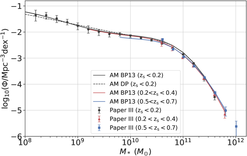
Figure 8: The galaxy stellar mass functions (solid lines) and $1\sigma$ errors (shadows) at different redshift ranges from the BP13 model. The results from the DP model at $z_{s}<0.2$ are also shown in dashed line. The model independent measurements of GSMF from Paper III are shown for comparison as dots with error bars.

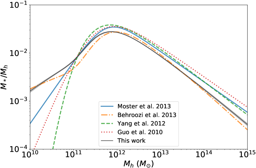
Figure 9: Comparison of the our mean stellar-halo mass function to previous studies at $z_{s}\sim 0.1$. Results compared include those from empirical modeling (Behroozi et al., 2013; Moster et al., 2013), from abundance matching (Guo et al., 2010) and from Conditional Stellar Mass Function (CSMF) modeling (Yang et al., 2012).

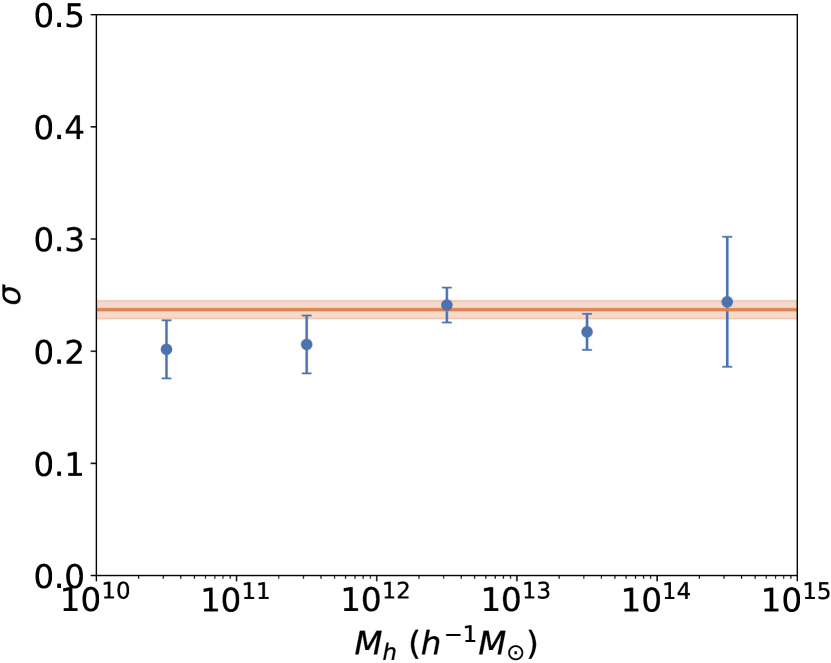
Figure 10: Halo mass dependence of the scatter in the SHMR at $z_{s}<0.2$. Blue dots with error bars show the results from the multi-$\sigma$ fittings. Orange line with shadow is the previous constraint with a single $\sigma$.

3.2 Subhalo Abundance Matching

To parameterize the SHMR, the most commonly used five-parameter formula is a double power law with a scatter (Wang & Jing, 2010; Yang et al., 2012; Moster et al., 2013):

$$M_{*}=\left[\frac{2k}{(M_{{\rm{acc}}}/{M_{0}})^{-\alpha}+(M_{{\rm{acc}}}/{M_{0}})^{-\beta}}\right]\,.$$ (8)

Here we define $M_{{\rm{acc}}}$ as the viral mass $M_{{\rm{vir}}}$ of the halo at the time when the galaxy was last the central dominant object. We use the fitting formula in Bryan & Norman (1998) to find $M_{{\rm{vir}}}$. The scatter in $\log(M_{*})$ at a given $M_{{\rm{acc}}}$ is described with a Gaussian function of the width $\sigma$. We also let $\alpha<\beta$ so that $\alpha$ and $\beta$ represent the slopes of the high and low mass ends of the SHMR respectively.

However, Behroozi et al. (2013) found that the SHMR of the double power law form (hereafter DP) fail to reproduce the upturn feature in the GSMF at $M_{*}<10^{9.5}M_{\odot}$. They provided a six-parameter formula (hereafter BP13) for the SHMR of low mass galaxies:

$$\log_{10}(M_{*})=\log_{10}(\epsilon M_{0})+f\left(\log_{10}\left(\frac{M_{{\rm{acc}}}}{M_{0}}\right)\right)-f(0)$$ (9)

$$f(x)=-\log_{10}(10^{-\beta x}+1)+\delta\frac{(\log_{10}(1+\exp{(x)}))^{\alpha}}{1+\exp{(10^{-x})}}\,,$$

with also a scatter $\sigma$ in $\log(M_{*})$. At $M_{{\rm{acc}}}\ll M_{0}$ and $M_{{\rm{acc}}}\gg M_{0}$, this formula degenerate into power laws with indices $\beta$ and $\alpha$.

We model the PAC measurements using both the BP13 and DP forms for the three redshift ranges. As we will show, both the BP13 and DP models are able to fit the measurements in the LOWZ and CMASS equally well, while the BP13 model is strongly favored to fit the measurements for $M_{*}<10^{10}M_{\odot}$ in the Main sample.

In simulation, the correlation functions are calculated using the tabulated method (Zheng & Guo, 2016; Gao et al., 2022) to avoid redundant computation in the fitting process. We define the $\chi^{2}$ as

$$\chi^{2}=\sum_{i=1}^{N_{\rm{m_{1}}}}\sum_{j=1}^{N_{\rm{m_{2}}}}(\mathcal{A}^{{\rm{PAC}}}_{i,j}-\mathcal{A}^{{\rm{AM}}}_{i,j})^{T}\mathbf{C}^{-1}_{i,j}(\mathcal{A}^{{\rm{PAC}}}_{i,j}-\mathcal{A}^{{\rm{AM}}}_{i,j})\,\,,$$ (10)

where $N_{{\rm{}_{m_{1}}}}$ and $N_{{\rm{}_{m_{2}}}}$ are the numbers of mass bins of ${\rm{pop}}_{1}$ and ${\rm{pop}}_{2}$, $\mathcal{A}^{{\rm{PAC}}}$ and $\mathcal{A}^{{\rm{AM}}}$ are the measurements and model predictions, $\mathbf{C}^{-1}$ is the inverse of the covariance matrix $\mathbf{C}$ and $T$ denotes matrix transposition. We use the Markov chain Monte Carlo (MCMC) sampler emcee (Foreman-Mackey et al., 2013) to perform maximum likelihood analyses of $\{M_{0},\alpha,\beta,k,\sigma\}$ for the DP model and $\{M_{0},\alpha,\delta,\beta,\epsilon,\sigma\}$ for the BP13 model.

3.3 Evolution of the Stellar-Halo Mass Relation

The marginalized posterior PDFs of the parameters are listed in Table 2 for the 3 redshift ranges and for both the BP13 and DP models, and we also show the joint posterior distributions of the parameters in Figure 15-20 using corner (Foreman-Mackey, 2016). The corresponding $\bar{n}_{2}w_{\rm{p}}(r_{\rm{p}})$ from the BP13 model in the 3 redshift ranges are shown as lines with shadows in Figure 3, 4 and 5. The fitting is good overall for all mass bins in our samples, and all the parameters are constrained well with percent or even sub-percent level errors. We also show the DP model fittings for the Main sample redshift range in Figure 6. We find that the DP model overpredicts the number of galaxies at $M_{*}=10^{9.5}M_{\odot}$ while underpredicts at $M_{*}<10^{8.6}M_{\odot}$. The BP13 model describes the SHMR for small galaxies better than the DP model.

The best-fit stellar-halo mass relations and the $1\sigma$ errors are shown in Figure 7. Results from the BP13 and DP models are shown by solid lines and dashed lines for $z_{s}<0.2$ (black), $0.2<z_{s}<0.4$ (red) and $0.5<z_{s}<0.7$ (blue). We also plot the stellar mass limit covered by the observation data at each redshift with the horizontal lines. In the mass ranges covered by the observation data, all the SHMRs are constrained to percent level, and the results from the BP13 and DP models are in good agreement with each other in the LOWZ and CMASS redshift ranges. However, as mentioned above, the DP model is unable to recover the upturn at the low mass end of the SHMR in the Main sample redshift range.

Our accurate SHMR determination shows that halos with a fixed mass at massive end ($M_{h}>M_{0}$) host more massive galaxies at higher redshift, which quantifies the downsizing of massive galaxies. On the other hand, our result indicates an opposite trend in the evolution for small halos ($M_{h}<M_{0}$), which means that small galaxies are continuously forming since $z_{s}=0.7$, although the conclusion must be treated with caution as the mass range covered by the observation data is limited for $M_{h}<M_{0}$ at $z_{s}=0.6$.

We also show the GSMFs in different redshift ranges derived from the BP13 model in Figure 8. The GSMFs from our model are all constrained to sub-percent level. The model independent measurements from Paper III are also plotted for comparison. We find that the two measurements are in good agreement with each other at all the 3 redshift ranges, proving that both measurements are robust in the whole mass range. At the massive end ($M_{*}>10^{11.0}M_{\odot}$), the results from Paper III were compared with the photoz results from the DESI Legacy Imaging Survey (Zhou et al., 2021) and we found great consistency (see Figure 5 there). Thus, the 3 independent measurements confirm that our measurements of the GSMF at the massive end are reliable. Our measurements indicate that the GSMF has nearly no evolution since $z_{s}=0.7$ for $M_{*}>10^{10.6}M_{\odot}$ and slightly increases with decreasing redshift for smaller stellar mass. We also list the GSMFs from the BP13 model in Table 3. We also plot the GSMF at $z_{s}<0.2$ from the DP model in Figure 8, it is clearly that the DP model fails to capture the upturn in the GSMF and the deviation starts from $10^{10.0}M_{\odot}$.

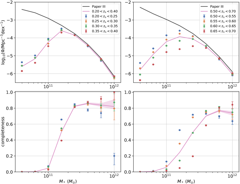
Figure 11: Top: GSMFs of the LOWZ (left) and CMASS (right) samples in different redshift ranges comparing to the DECaLS photoz measurements in Paper III ($0.2<z_{p}<0.4$ and $0.5<z_{p}<0.7$). Bottom: stellar mass completeness of the LOWZ (left) and CMASS (right) samples.

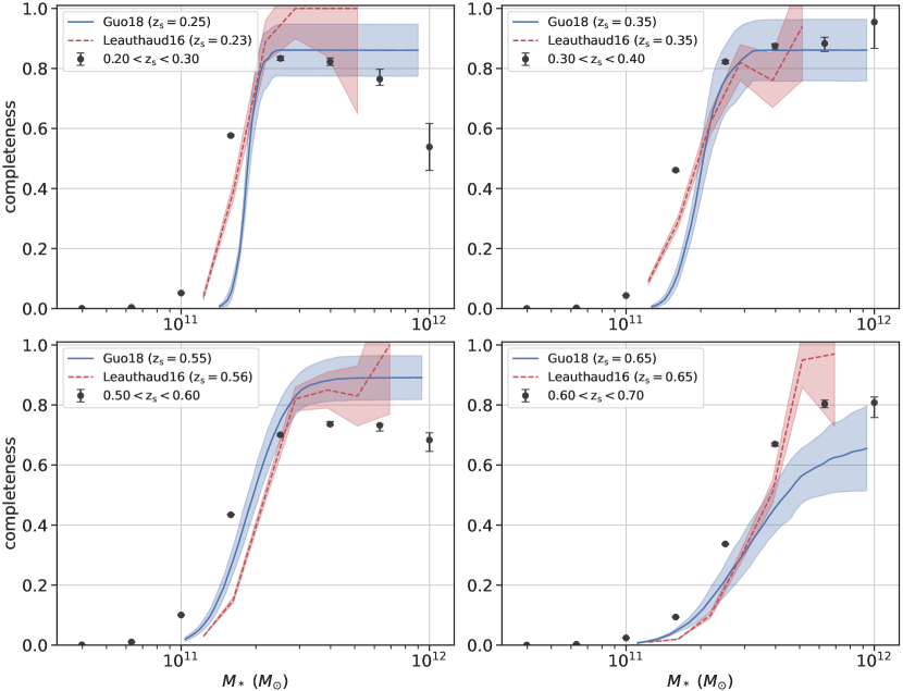
Figure 12: Stellar mass completeness comparing to the results from Leauthaud et al. (2016) and Guo et al. (2018).

Combining the SHMR and GSMF measurements, our results favor the physical picture that massive galaxies are quenched since at least $z_{s}=0.7$ while their host halos are still assembling their mass, and that low mass galaxies are still forming stars in an efficient way. Our results are inconsistent with a few previous works (Moster et al., 2013; Behroozi et al., 2013, 2019) for massive galaxies and halos. In these works, the stellar mass increases with decreasing redshift for fixed halo mass at $M_{h}>M_{0}$. It may be due to that the GSMFs they used to constrain the SHMR at different redshifts are not well calibrated. Their GSMFs are still increasing with decreasing redshift at the massive ends. Their GSMFs are usually from different surveys that may have systematic bias between each other. Due to the exponentially decreasing feature of the GSMF at the massive end, a very small offset can cause a significant change in the GSMF. As we mentioned in Paper III (See Appendix C there), at the high mass end, the GSMF of the north and south parts of the DESI Legacy Imaging Surveys can still have a $30\%$ offset with already a $500\ {\rm{deg}}^{2}$ footprint overlapped for calibration. Different methods for source extraction, photometry and SED can also introduce further bias. Moreover, the GSMFs they used at high redshifts are usually from the deep spectroscopic or photometric surveys with relatively small survey areas, thus the cosmic variance may become important for the massive end. One of the advantages for measuring the SHMR using PAC is that we can provide measurements in a uniform way, and we can minimize the systematic bias between different redshifts.

In Figure 9, we compare our measurement of SHMR to previous studies at $z_{s}\sim 0.1$. In these works, Behroozi et al. (2013) and Moster et al. (2013) collected the GSMF and/or cosmic star formation rate measurements from different surveys and modeled the evolution of the SHMR using empirical modeling, Guo et al. (2010) modeled the SHMR in the local universe with the SDSS DR7 GSMF (Li & White, 2009) and galaxy correlations using abundance matching, and Yang et al. (2012) constrained the evolution of SHMR based on the GSMF and conditional stellar mass function (CSMF, Yang et al., 2009) measurements at different redshifts. The halo masses are all corrected to $M_{{\rm{vir}}}$. However, there are still some differences in the definition of subhalo mass. For satellites, Behroozi et al. (2013) and Moster et al. (2013) use the peak progenitor mass ($M_{{\rm{peak}}}$) while others use the last accretion mass ($M_{\rm{acc}}$). Here we assume that the definition of the subhalo mass has a negligible effect.

At the high mass end, results from different studies are relatively consistent, since the measurements are robust for this mass range with the large area spectroscopic surveys, though discrepancies still exist that may be due to some systematics in the measurements of the stellar mass. At the low mass end, the discrepancies between studies are large, since the constraints are mainly from the GSMF measurements in SDSS, which have a very limit volume ($z_{s}<0.03$) for low mass galaxies ($M_{*}<10^{9.0}M_{\odot}$). Instead, making full use of the deep photometric data, we can give a precise measurement of the SHMR at the low mass end with PAC.

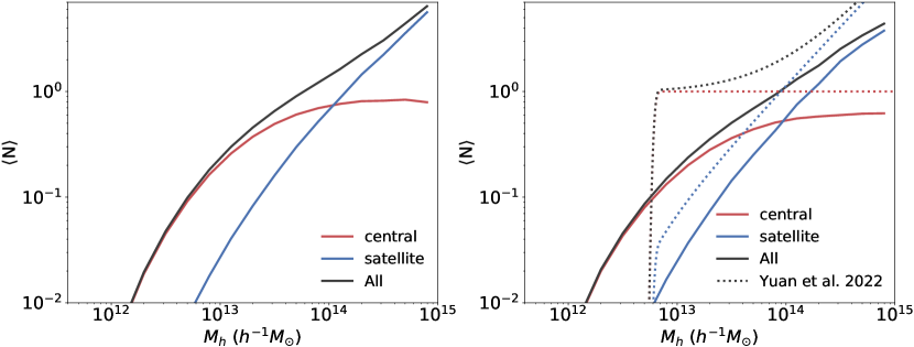
Figure 13: HODs of the LOWZ (left) and CMASS (right) samples derived from our SHMR after taking the stellar mass completeness into account. The HOD of the CMASS sample from Yuan et al. (2022a) are also presented for comparison.

3.4 Halo Mass Dependence of the Scatter

The SHMR models we used above adopt a constant scatter $\sigma$. However, whether the scatter depends on halo mass or not is still under debate. Thus, we model the PAC measurements at $z_{s}<0.2$ again with the BP13 model but with 5 different scatters for the halo mass ranges of $[10^{10.0},10^{11.0}]h^{-1}M_{\odot}$, $[10^{11.0},10^{12.0}]h^{-1}M_{\odot}$, $[10^{12.0},10^{13.0}]h^{-1}M_{\odot}$, $[10^{13.0},10^{14.0}]h^{-1}M_{\odot}$ and $[10^{14.0},10^{15.0}]h^{-1}M_{\odot}$, respectively. The results are shown in Figure 10. With the very accurate measurements, we find nearly no dependence of the scatter on halo mass down to $10^{10.0}h^{-1}M_{\odot}$. The scatters are all within $0.2-0.25$ and are consistent with the results from the previous single scatter model.

4 Halo Occupation Distributions of the LOWZ and CMASS LRG Samples

The halo occupation distributions (HOD) of the LOWZ and CMASS samples are still under debate (Leauthaud et al., 2016; Guo et al., 2018) due to the stellar mass incompleteness, and the reliability of the HOD can influence cosmology studies such as galaxy-galaxy lensing and redshift space distortion. With the GSMF measured in Paper III and the SHMR measured in this work, we can derive the stellar mass incompleteness and the HODs for the LOWZ and CMASS samples.

4.1 Stellar Mass Completeness

We first calculate the stellar mass completeness for the LOWZ and CMASS samples. We adopt the GSMFs measured in Paper III as complete references. For $M_{*}=10^{12}M_{\odot}$, as discussed in Paper III (see Figure 5), the photoz measurement of GSMFs is more reliable and adopted here, because the number of so massive galaxies is very limited in the survey for the two-point statistics.

We present the GSMFs of the LOWZ and CMASS samples in different redshift ranges in the top panels of Figure 11 along with our GSMFs in Paper III. Then we derive the stellar mass completeness in the bottom panels and also list them in Table 4. Errors are all estimated using jackknife-resampling. The completeness in general increases with stellar mass and is peaked at around $10^{11.6}M_{\odot}$. The peak completeness is around $85\%$ for the LOWZ and around $80\%$ for the CMASS. Both the LOWZ and the CMASS samples are not complete even at the highest stellar mass $M_{*}=10^{11.8}M_{\odot}$ and $10^{12.0}M_{\odot}$, and the incompleteness is even worse at the $10^{12.0}M_{\odot}$ especially at the lower redshift bins ($z_{s}=0.25$ for the LOWZ and $z_{s}=0.55$ for the CMASS). In Table 5, we mimic the target selection process for the CMASS sample of $10^{11.8}M_{\odot}$ and $10^{12.0}M_{\odot}$ using the DECaLS photoz sample. We find that target selection for the spectroscopic observations drops out $11.5\%$ and $11.2\%$ of galaxies, and only $89.7\%$ and $81.3\%$ of the selected sources have successful redshift measurements. The two effects combined result in about $79\%$ and $76\%$ completeness, which is consistent with our measurement in Figure 11. Therefor, at least for CMASS, the lower completeness at $10^{12.0}M_{\odot}$ may be due to less spectral identification.

We also compare our stellar mass completeness with previous works (Leauthaud et al., 2016; Guo et al., 2018) in Figure 12. Qualitatively the three studies yield similar incompleteness trends. Quantitatively, the results for LOWZ from the different studies are consistent with each other, while the differences are larger for CMASS. The reason for the differences is not clear. Their results might be sensitive to the total GSMFs used in Leauthaud et al. (2016) and the formula used to model the completeness in Guo et al. (2018).

4.2 Halo Occupation Distribution

Combining with the stellar mass completeness, we can derive the HODs for the LOWZ and CMASS samples from our SHMR. We use the completeness in the redshift ranges of $0.2<z_{s}<0.4$ and $0.5<z_{s}<0.7$ for LOWZ and CMASS samples respectively, and assume that the galaxies are randomly selected. The HODs for the LOWZ and CMASS samples are shown in Figure 13.

As an example, we also compare with a recent HOD for CMASS galaxies (dotted lines in Figure 13) presented by Yuan et al. (2022a) who adopted the standard form of Zheng et al. (2007). Yuan et al. (2022a) constrained the cosmological parameters and HOD parameters simultaneously using the emulator based on the ABACUSHOD framework (Yuan et al., 2022b) in the ABACUSSUMMIT simulation suite (Maksimova et al., 2021). We find that both the amplitude and shape of our HOD are different from those of Yuan et al. (2022a). The difference might be mainly caused by the fact that they did not consider the stellar mass incompleteness. It would be interesting to investigate how much the incompleteness would impact on the determination of cosmological parameters. Cosmological probes, such as galaxy-galaxy lensing and redshift space distortion, are especially sensitive to the HOD or the stellar mass completeness. With the accurately measured SHMR and stellar mass completeness, we will revisit this question in a future work.

5 Summary

In this work, using the SDSS Main, LOWZ and CMASS spectroscopic samples and DECaLS photometric data, we measure $\bar{n}_{2}w_{{\rm{p}}}$ down to stellar mass $10^{8.0}M_{\odot}$, $10^{9.2}M_{\odot}$ and $10^{9.8}M_{\odot}$ for redshift ranges $z_{s}<0.2$, $0.2<z_{s}<0.4$ and $0.5<z_{s}<0.7$, respectively. We model the $\bar{n}_{2}w_{{\rm{p}}}$ with the abundance matching method in N-body simulation and accurately constrain the evolution of SHMR. We summarize our results as follows:

• The parameters of the SHMRs are all well constrained (percent level) for the redshift ranges . According to our results, halos with a fixed halo mass host more massive galaxies at higher redshift for the high mass end ($M_{h}>M_{0}$), and the trend is reversed at the low mass end ($M_{h}<M_{0}$). This quantifies the downsizing of massive galaxies since $z_{s}=0.7$, and indicates that small galaxies are still growing faster than their host halos.

• With our precise measurement of $\bar{n}_{2}w_{{\rm{p}}}$ down to stellar mass $10^{8.0}M_{\odot}$ in the local universe ($z_{s}<0.2$), we find the form of Behroozi et al. (2013) describes the SHMR at low mass much better than the double power law form.

• Adopting a halo mass dependent scatter of SHMR, we demonstrated that the scatter does not vary with halo mass in the wide mass range of $[10^{10.0},10^{15.0}]h^{-1}M_{\odot}$ at high precision, which supports that a constant scatter assumed in many previous studies is good approximation.

• The derived GSMFs from our SHMRs are in perfect agreement with the model independent measurements in Paper III at all three redshifts, but the present study extends the GSMF measurement to lower stellar mass. Our results show that the GSMF has little evolution at the massive end $M_{*}>10^{10.5}M_{\odot}$ since $z_{s}=0.7$.

• With the accurate SHMR and GSMF measurements, we calculate the stellar mass completeness and HODs for the LOWZ and CMASS samples. We find that the standard HOD modeling may lead to a biased result without properly taking into account the stellar mass completeness. Our SHMR and stellar mass completeness measurements will be useful in correctly interpreting the cosmological measurements such as modeling galaxy-galaxy lensing and redshift space distortion based on these samples.

With the next generation larger and deeper spectroscopic and photometric surveys such as Dark Energy Spectroscopic Instrument (DESI Collaboration et al., 2016), Legacy Survey of Space and Time (Ivezić et al., 2019) and Euclid (Laureijs et al., 2011), we can use the PAC method to explore the galaxy-halo connection to higher redshift and lower mass.

Appendix A verifying the completeness

Figure 14: PAC measurements for ${\rm{pop}}_{1}=10^{11.2}M_{\odot}$ and ${\rm{pop}}_{2}=10^{8.6}M_{\odot}$ at $z_{s}<0.2$ (blue) and $z_{s}<0.15$ (orange).

We verify our method of determining the mass limits by comparing the $\bar{n}_{2}w_{\rm{p}}$ measurements between $z_{s}<0.2$ (4 redshift bins) and $z_{s}<0.15$ (3 redshift bins) for ${\rm{pop}}_{1}=10^{11.2}M_{\odot}$ and ${\rm{pop}}_{2}=10^{8.6}M_{\odot}$. According to our results, for DECaLS, galaxies with $10^{8.6}M_{\odot}$ are exactly complete at $z_{s}=0.2$ while galaxies with $10^{8.4}M_{\odot}$ are only complete at $z_{s}=0.15$. If $10^{8.6}M_{\odot}$ is still not complete at $z_{s}=0.2$, the measured $\bar{n}_{2}w_{\rm{p}}$ from $z_{s}<0.2$ will be lower than that from $z_{s}<0.15$. However, as shown in Figure 14, there is no systematic differences between the results from the two redshift ranges, verifying that $10^{8.6}M_{\odot}$ is complete at $z_{s}=0.2$ for DECaLS.

Appendix B Posterior distributions of the parameters

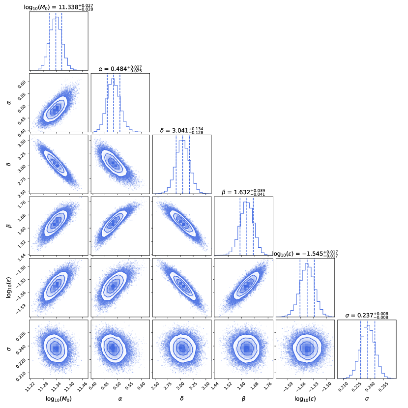
Figure 15: Posterior distributions of the parameters in the BP13 model in the Main sample redshift range ($z_{s}<0.2$). The central value is a median, and the error means $16\sim 84$ percentiles after other parameters are marginalized over.

Figure 16: The same as Figure 15 but for the BP13 model in the LOWZ redshift range ($0.2<z_{s}<0.4$).

Figure 17: The same as Figure 15 but for the BP13 model in the CMASS redshift range ($0.5<z_{s}<0.7$).

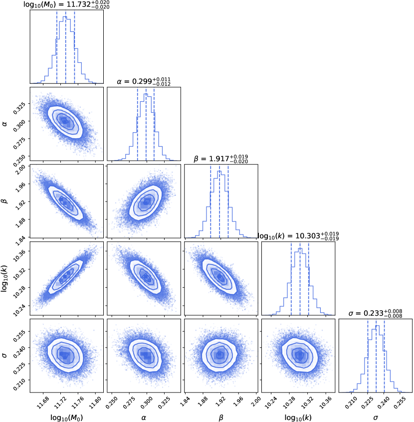
Figure 18: Posterior distributions of the parameters in the DP model in the Main sample redshift range ($z_{s}<0.2$). The central value is a median, and the error means $16\sim 84$ percentiles after other parameters are marginalized over.

Figure 19: The same as Figure 18 but for the DP model in the LOWZ redshift range ($0.2<z_{s}<0.4$).

Figure 20: The same as Figure 18 but for the DP model in the CMASS redshift range ($0.5<z_{s}<0.7$).

We show the posterior distributions of the parameters of the BP13 model at the Main, LOWZ and CMASS redshift ranges in Figure 15, 16 and 17. The results of the DP model are also displayed in Figure 18, 19 and 20.

Appendix C The GSMFs from AM in Tabular form

Table 3: The galaxy stellar mass functions $\log_{10}(\Phi/{\rm{Mpc^{-3}dex^{-1})}}$ at different redshifts from the BP13 model.

$\log_{10}(M_{*}/M_{\odot})$	$z_{s}<0.2$	$0.2<z_{s}<0.4$	$0.5<z_{s}<0.7$
8.0	$-1.227_{-0.013}^{+0.012}$
8.2	$-1.310_{-0.014}^{+0.012}$
8.4	$-1.412_{-0.011}^{+0.010}$
8.6	$-1.524_{-0.009}^{+0.008}$
8.8	$-1.642_{-0.009}^{+0.009}$
9.0	$-1.758_{-0.010}^{+0.009}$
9.2	$-1.863_{-0.010}^{+0.008}$	$-1.890_{-0.008}^{+0.010}$
9.4	$-1.951_{-0.009}^{+0.006}$	$-1.973_{-0.007}^{+0.009}$
9.6	$-2.022_{-0.009}^{+0.006}$	$-2.040_{-0.005}^{+0.008}$
9.8	$-2.078_{-0.010}^{+0.006}$	$-2.096_{-0.005}^{+0.008}$	$-2.205_{-0.008}^{+0.008}$
10.0	$-2.124_{-0.010}^{+0.007}$	$-2.144_{-0.006}^{+0.009}$	$-2.243_{-0.007}^{+0.007}$
10.2	$-2.170_{-0.010}^{+0.007}$	$-2.195_{-0.006}^{+0.009}$	$-2.277_{-0.006}^{+0.007}$
10.4	$-2.232_{-0.008}^{+0.007}$	$-2.268_{-0.007}^{+0.008}$	$-2.324_{-0.006}^{+0.007}$
10.6	$-2.337_{-0.007}^{+0.007}$	$-2.389_{-0.008}^{+0.008}$	$-2.417_{-0.007}^{+0.007}$
10.8	$-2.513_{-0.008}^{+0.009}$	$-2.586_{-0.008}^{+0.008}$	$-2.592_{-0.009}^{+0.007}$
11.0	$-2.787_{-0.010}^{+0.011}$	$-2.878_{-0.008}^{+0.009}$	$-2.869_{-0.009}^{+0.007}$
11.2	$-3.177_{-0.013}^{+0.012}$	$-3.266_{-0.008}^{+0.011}$	$-3.247_{-0.010}^{+0.008}$
11.4	$-3.693_{-0.020}^{+0.016}$	$-3.751_{-0.009}^{+0.013}$	$-3.721_{-0.011}^{+0.011}$
11.6	$-4.347_{-0.035}^{+0.026}$	$-4.343_{-0.014}^{+0.018}$	$-4.291_{-0.017}^{+0.019}$
11.8		$-5.070_{-0.025}^{+0.028}$	$-4.979_{-0.031}^{+0.037}$

In Table 3, we list the GSMFs inferred from our constrained BP13 abundance matching model for the 3 redshift ranges $z_{s}<0.2$, $0.2<z_{s}<0.4$ and $0.5<z_{s}<0.7$. The GSMFs are all constrained to sub-percent level.

Appendix D stellar mass completeness of the LOWZ and CMASS samples

Table 4: Logarithmic ($\log_{10}$) stellar mass completeness of the LOWZ and CMASS samples at different redshift ranges.

$z_{s}$	$10^{10.6}M_{\odot}$	$10^{10.8}M_{\odot}$	$10^{11.0}M_{\odot}$	$10^{11.2}M_{\odot}$	$10^{11.4}M_{\odot}$	$10^{11.6}M_{\odot}$
	$10^{11.8}M_{\odot}$	$10^{12.0}M_{\odot}$
$0.20-0.40$	$-3.090\pm 0.014$	$-2.496\pm 0.008$	$-1.333\pm 0.003$	$-0.299\pm 0.002$	$-0.083\pm 0.003$	$-0.067\pm 0.004$
	$-0.076\pm 0.010$	$-0.086\pm 0.031$
$0.20-0.25$	$-2.862\pm 0.029$	$-2.313\pm 0.016$	$-1.140\pm 0.006$	$-0.182\pm 0.003$	$-0.072\pm 0.005$	$-0.110\pm 0.010$
	$-0.132\pm 0.023$	$-0.697\pm 0.136$
$0.25-0.30$	$-3.050\pm 0.028$	$-2.449\pm 0.015$	$-1.422\pm 0.008$	$-0.282\pm 0.003$	$-0.085\pm 0.005$	$-0.071\pm 0.008$
	$-0.092\pm 0.021$	$-0.099\pm 0.070$
$0.30-0.35$	$-3.052\pm 0.024$	$-2.446\pm 0.014$	$-1.198\pm 0.005$	$-0.262\pm 0.003$	$-0.081\pm 0.004$	$-0.063\pm 0.007$
	$-0.079\pm 0.016$	$-0.059\pm 0.054$
$0.35-0.40$	$-3.338\pm 0.029$	$-2.724\pm 0.020$	$-1.555\pm 0.006$	$-0.405\pm 0.003$	$-0.090\pm 0.003$	$-0.058\pm 0.007$
	$-0.038\pm 0.017$	$-0.001\pm 0.044$
$0.50-0.70$	$-3.244\pm 0.010$	$-2.211\pm 0.003$	$-1.237\pm 0.002$	$-0.611\pm 0.001$	$-0.303\pm 0.002$	$-0.154\pm 0.003$
	$-0.114\pm 0.006$	$-0.132\pm 0.014$
$0.50-0.55$	$-2.862\pm 0.012$	$-1.888\pm 0.007$	$-0.888\pm 0.002$	$-0.280\pm 0.002$	$-0.144\pm 0.003$	$-0.135\pm 0.005$
	$-0.158\pm 0.012$	$-0.196\pm 0.029$
$0.55-0.60$	$-3.159\pm 0.017$	$-2.094\pm 0.007$	$-1.128\pm 0.003$	$-0.450\pm 0.002$	$-0.164\pm 0.003$	$-0.126\pm 0.005$
	$-0.117\pm 0.010$	$-0.142\pm 0.027$
$0.60-0.65$	$-3.521\pm 0.025$	$-2.401\pm 0.008$	$-1.468\pm 0.004$	$-0.848\pm 0.003$	$-0.310\pm 0.003$	$-0.116\pm 0.004$
	$-0.089\pm 0.008$	$-0.126\pm 0.026$
$0.65-0.70$	$-3.822\pm 0.033$	$-2.786\pm 0.013$	$-1.823\pm 0.006$	$-1.311\pm 0.005$	$-0.707\pm 0.004$	$-0.234\pm 0.005$
	$-0.094\pm 0.009$	$-0.074\pm 0.022$

In Table 4, we list the stellar mass completeness of the LOWZ and CMASS samples at different redshift ranges.

Table 5: Numbers of galaxies with $10^{11.8}M_{\odot}$ and $10^{12.0}M_{\odot}$ after each target selection step of CMASS using DECaLS photoz sample at $0.5<z_{p}<0.7$.

Steps	$10^{11.8}M_{\odot}$	$10^{12.0}M_{\odot}$
DECaLS	$10824$	$1484$
SDSS photometry matched	10467	1403
low-z cut: $|d_{\perp}|>0.55$a	10320	1375
constant mass cut: $i_{{\rm{cmod}}}<19.86+1.6(d_{\perp}-0.8)$	10123	1364
magnitude limit cut: $17.5<i_{{\rm{cmod}}}<19.9$	9953	1354
problematic deblending cut: $r_{{\rm{mod}}}-i_{{\rm{mod}}}<2$	9868	1340
magnitude limit cut: $i_{{\rm{fib2}}}<21.5$b	9655	1328
star–galaxy separation: $i_{{\rm{psf}}}-i_{{\rm{mod}}}>0.2+0.2(20.0-i_{{\rm{mod}}})$	9637	1327
star–galaxy separation: $z_{{\rm{psf}}}-z_{{\rm{mod}}}>9.125-0.46z_{{\rm{mod}}}$	9581	1318
CMASS matchedc	8598 (79%)	1123 (76%)

• $|d_{\perp}|=(r_{{\rm{mod}}}-i_{{\rm{mod}}})-(g_{{\rm{mod}}}-r_{{\rm{mod}}})/8$

• $i_{{\rm{fib2}}}$ is the expected $i$ band magnitude through the SDSS-III 2 arcsec fibres.

• Since the footprint of the CMASS sample is slightly smaller than the SDSS photometric sample, the number is corrected using the area ratio.

In Table 5, we simulate the target selection process of the CMASS sample with $10^{11.8}M_{\odot}$ and $10^{12.0}M_{\odot}$ using the DECaLS photoz sample at $0.5<z_{p}<0.7$. Notice that the completeness accounts well for the results presented in Figure 12.

References

- Abazajian et al. (2009) Abazajian, K. N., Adelman-McCarthy, J. K., Agüeros, M. A., et al. 2009, ApJS, 182, 543, doi: 10.1088/0067-0049/182/2/543
- Ahn et al. (2012) Ahn, C. P., Alexandroff, R., Allende Prieto, C., et al. 2012, ApJS, 203, 21, doi: 10.1088/0067-0049/203/2/21
- Ahumada et al. (2020) Ahumada, R., Prieto, C. A., Almeida, A., et al. 2020, ApJS, 249, 3, doi: 10.3847/1538-4365/ab929e
- Alam et al. (2015) Alam, S., Albareti, F. D., Allende Prieto, C., et al. 2015, ApJS, 219, 12, doi: 10.1088/0067-0049/219/1/12
- Baldry et al. (2008) Baldry, I. K., Glazebrook, K., & Driver, S. P. 2008, MNRAS, 388, 945, doi: 10.1111/j.1365-2966.2008.13348.x
- Bartelmann & Schneider (2001) Bartelmann, M., & Schneider, P. 2001, Phys. Rep., 340, 291, doi: 10.1016/S0370-1573(00)00082-X
- Behroozi et al. (2019) Behroozi, P., Wechsler, R. H., Hearin, A. P., & Conroy, C. 2019, MNRAS, 488, 3143, doi: 10.1093/mnras/stz1182
- Behroozi et al. (2013) Behroozi, P. S., Wechsler, R. H., & Conroy, C. 2013, ApJ, 770, 57, doi: 10.1088/0004-637X/770/1/57
- Berlind & Weinberg (2002) Berlind, A. A., & Weinberg, D. H. 2002, ApJ, 575, 587, doi: 10.1086/341469
- Bolton et al. (2012) Bolton, A. S., Schlegel, D. J., Aubourg, É., et al. 2012, AJ, 144, 144, doi: 10.1088/0004-6256/144/5/144
- Boquien et al. (2019) Boquien, M., Burgarella, D., Roehlly, Y., et al. 2019, A&A, 622, A103, doi: 10.1051/0004-6361/201834156
- Brammer et al. (2008) Brammer, G. B., van Dokkum, P. G., & Coppi, P. 2008, ApJ, 686, 1503, doi: 10.1086/591786
- Bruzual & Charlot (2003) Bruzual, G., & Charlot, S. 2003, MNRAS, 344, 1000, doi: 10.1046/j.1365-8711.2003.06897.x
- Bryan & Norman (1998) Bryan, G. L., & Norman, M. L. 1998, ApJ, 495, 80, doi: 10.1086/305262
- Calzetti et al. (2000) Calzetti, D., Armus, L., Bohlin, R. C., et al. 2000, ApJ, 533, 682, doi: 10.1086/308692
- Chabrier (2003) Chabrier, G. 2003, PASP, 115, 763, doi: 10.1086/376392
- Cole et al. (2001) Cole, S., Norberg, P., Baugh, C. M., et al. 2001, MNRAS, 326, 255, doi: 10.1046/j.1365-8711.2001.04591.x
- Colless et al. (2001) Colless, M., Dalton, G., Maddox, S., et al. 2001, MNRAS, 328, 1039, doi: 10.1046/j.1365-8711.2001.04902.x
- Dark Energy Survey Collaboration et al. (2016) Dark Energy Survey Collaboration, Abbott, T., Abdalla, F. B., et al. 2016, MNRAS, 460, 1270, doi: 10.1093/mnras/stw641
- Davidzon et al. (2013) Davidzon, I., Bolzonella, M., Coupon, J., et al. 2013, A&A, 558, A23, doi: 10.1051/0004-6361/201321511
- Davidzon et al. (2017) Davidzon, I., Ilbert, O., Laigle, C., et al. 2017, A&A, 605, A70, doi: 10.1051/0004-6361/201730419
- Davis et al. (2003) Davis, M., Faber, S. M., Newman, J., et al. 2003, in Society of Photo-Optical Instrumentation Engineers (SPIE) Conference Series, Vol. 4834, Discoveries and Research Prospects from 6- to 10-Meter-Class Telescopes II, ed. P. Guhathakurta, 161–172, doi: 10.1117/12.457897
- DESI Collaboration et al. (2016) DESI Collaboration, Aghamousa, A., Aguilar, J., et al. 2016, arXiv e-prints, arXiv:1611.00036. https://arxiv.org/abs/1611.00036
- Dey et al. (2019) Dey, A., Schlegel, D. J., Lang, D., et al. 2019, AJ, 157, 168, doi: 10.3847/1538-3881/ab089d
- Driver et al. (2022) Driver, S. P., Bellstedt, S., Robotham, A. S. G., et al. 2022, MNRAS, 513, 439, doi: 10.1093/mnras/stac472
- Fontana et al. (2006) Fontana, A., Salimbeni, S., Grazian, A., et al. 2006, A&A, 459, 745, doi: 10.1051/0004-6361:20065475
- Foreman-Mackey (2016) Foreman-Mackey, D. 2016, The Journal of Open Source Software, 1, 24, doi: 10.21105/joss.00024
- Foreman-Mackey et al. (2013) Foreman-Mackey, D., Hogg, D. W., Lang, D., & Goodman, J. 2013, PASP, 125, 306, doi: 10.1086/670067
- Frenk & White (2012) Frenk, C. S., & White, S. D. M. 2012, Annalen der Physik, 524, 507, doi: 10.1002/andp.201200212
- Gao et al. (2022) Gao, H., Jing, Y. P., Zheng, Y., & Xu, K. 2022, ApJ, 928, 10, doi: 10.3847/1538-4357/ac501b
- Garilli et al. (2014) Garilli, B., Guzzo, L., Scodeggio, M., et al. 2014, A&A, 562, A23, doi: 10.1051/0004-6361/201322790
- Guo et al. (2018) Guo, H., Yang, X., & Lu, Y. 2018, ApJ, 858, 30, doi: 10.3847/1538-4357/aabc56
- Guo et al. (2010) Guo, Q., White, S., Li, C., & Boylan-Kolchin, M. 2010, MNRAS, 404, 1111, doi: 10.1111/j.1365-2966.2010.16341.x
- Han et al. (2018) Han, J., Cole, S., Frenk, C. S., Benitez-Llambay, A., & Helly, J. 2018, MNRAS, 474, 604, doi: 10.1093/mnras/stx2792
- Han et al. (2012) Han, J., Jing, Y. P., Wang, H., & Wang, W. 2012, MNRAS, 427, 2437, doi: 10.1111/j.1365-2966.2012.22111.x
- Hartley et al. (2022) Hartley, W. G., Choi, A., Amon, A., et al. 2022, MNRAS, 509, 3547, doi: 10.1093/mnras/stab3055
- Hinshaw et al. (2013) Hinshaw, G., Larson, D., Komatsu, E., et al. 2013, ApJS, 208, 19, doi: 10.1088/0067-0049/208/2/19
- Ilbert et al. (2013) Ilbert, O., McCracken, H. J., Le Fèvre, O., et al. 2013, A&A, 556, A55, doi: 10.1051/0004-6361/201321100
- Ivezić et al. (2019) Ivezić, Ž., Kahn, S. M., Tyson, J. A., et al. 2019, ApJ, 873, 111, doi: 10.3847/1538-4357/ab042c
- Jiang et al. (2008) Jiang, C. Y., Jing, Y. P., Faltenbacher, A., Lin, W. P., & Li, C. 2008, ApJ, 675, 1095, doi: 10.1086/526412
- Jing (2019) Jing, Y. 2019, Science China Physics, Mechanics, and Astronomy, 62, 19511, doi: 10.1007/s11433-018-9286-x
- Jing et al. (1998) Jing, Y. P., Mo, H. J., & Börner, G. 1998, ApJ, 494, 1, doi: 10.1086/305209
- Jing & Suto (2002) Jing, Y. P., & Suto, Y. 2002, ApJ, 574, 538, doi: 10.1086/341065
- Kaiser (1987) Kaiser, N. 1987, MNRAS, 227, 1, doi: 10.1093/mnras/227.1.1
- Landy & Szalay (1993) Landy, S. D., & Szalay, A. S. 1993, ApJ, 412, 64, doi: 10.1086/172900
- Lang et al. (2016) Lang, D., Hogg, D. W., & Mykytyn, D. 2016, The Tractor: Probabilistic astronomical source detection and measurement, Astrophysics Source Code Library, record ascl:1604.008. http://ascl.net/1604.008
- Laureijs et al. (2011) Laureijs, R., Amiaux, J., Arduini, S., et al. 2011, arXiv e-prints, arXiv:1110.3193. https://arxiv.org/abs/1110.3193
- Le Fèvre et al. (2005) Le Fèvre, O., Vettolani, G., Garilli, B., et al. 2005, A&A, 439, 845, doi: 10.1051/0004-6361:20041960
- Leauthaud et al. (2016) Leauthaud, A., Bundy, K., Saito, S., et al. 2016, MNRAS, 457, 4021, doi: 10.1093/mnras/stw117
- Leja et al. (2020) Leja, J., Speagle, J. S., Johnson, B. D., et al. 2020, ApJ, 893, 111, doi: 10.3847/1538-4357/ab7e27
- Li et al. (2006) Li, C., Kauffmann, G., Jing, Y. P., et al. 2006, MNRAS, 368, 21, doi: 10.1111/j.1365-2966.2006.10066.x
- Li & White (2009) Li, C., & White, S. D. M. 2009, MNRAS, 398, 2177, doi: 10.1111/j.1365-2966.2009.15268.x
- Ma & Fry (2000) Ma, C.-P., & Fry, J. N. 2000, ApJ, 543, 503, doi: 10.1086/317146
- Maksimova et al. (2021) Maksimova, N. A., Garrison, L. H., Eisenstein, D. J., et al. 2021, MNRAS, 508, 4017, doi: 10.1093/mnras/stab2484
- Marulli et al. (2013) Marulli, F., Bolzonella, M., Branchini, E., et al. 2013, A&A, 557, A17, doi: 10.1051/0004-6361/201321476
- McLeod et al. (2021) McLeod, D. J., McLure, R. J., Dunlop, J. S., et al. 2021, MNRAS, 503, 4413, doi: 10.1093/mnras/stab731
- Meneux et al. (2008) Meneux, B., Guzzo, L., Garilli, B., et al. 2008, A&A, 478, 299, doi: 10.1051/0004-6361:20078182
- Mo et al. (2010) Mo, H., van den Bosch, F. C., & White, S. 2010, Galaxy Formation and Evolution (Cambridge University Press)
- Mortlock et al. (2015) Mortlock, A., Conselice, C. J., Hartley, W. G., et al. 2015, MNRAS, 447, 2, doi: 10.1093/mnras/stu2403
- Mostek et al. (2013) Mostek, N., Coil, A. L., Cooper, M., et al. 2013, ApJ, 767, 89, doi: 10.1088/0004-637X/767/1/89
- Moster et al. (2013) Moster, B. P., Naab, T., & White, S. D. M. 2013, MNRAS, 428, 3121, doi: 10.1093/mnras/sts261
- Moster et al. (2018) —. 2018, MNRAS, 477, 1822, doi: 10.1093/mnras/sty655
- Muzzin et al. (2013) Muzzin, A., Marchesini, D., Stefanon, M., et al. 2013, ApJ, 777, 18, doi: 10.1088/0004-637X/777/1/18
- Naab & Ostriker (2017) Naab, T., & Ostriker, J. P. 2017, ARA&A, 55, 59, doi: 10.1146/annurev-astro-081913-040019
- Norberg et al. (2002) Norberg, P., Baugh, C. M., Hawkins, E., et al. 2002, MNRAS, 332, 827, doi: 10.1046/j.1365-8711.2002.05348.x
- Peacock & Smith (2000) Peacock, J. A., & Smith, R. E. 2000, MNRAS, 318, 1144, doi: 10.1046/j.1365-8711.2000.03779.x
- Pozzetti et al. (2007) Pozzetti, L., Bolzonella, M., Lamareille, F., et al. 2007, A&A, 474, 443, doi: 10.1051/0004-6361:20077609
- Reid et al. (2016) Reid, B., Ho, S., Padmanabhan, N., et al. 2016, MNRAS, 455, 1553, doi: 10.1093/mnras/stv2382
- Schlegel et al. (1998) Schlegel, D. J., Finkbeiner, D. P., & Davis, M. 1998, ApJ, 500, 525, doi: 10.1086/305772
- Scoccimarro (2004) Scoccimarro, R. 2004, Phys. Rev. D, 70, 083007, doi: 10.1103/PhysRevD.70.083007
- Seljak (2000) Seljak, U. 2000, MNRAS, 318, 203, doi: 10.1046/j.1365-8711.2000.03715.x
- Shuntov et al. (2022) Shuntov, M., McCracken, H. J., Gavazzi, R., et al. 2022, A&A, 664, A61, doi: 10.1051/0004-6361/202243136
- Somerville & Davé (2015) Somerville, R. S., & Davé, R. 2015, ARA&A, 53, 51, doi: 10.1146/annurev-astro-082812-140951
- Steidel et al. (2003) Steidel, C. C., Adelberger, K. L., Shapley, A. E., et al. 2003, ApJ, 592, 728, doi: 10.1086/375772
- Takada et al. (2014) Takada, M., Ellis, R. S., Chiba, M., et al. 2014, PASJ, 66, R1, doi: 10.1093/pasj/pst019
- Tomczak et al. (2014) Tomczak, A. R., Quadri, R. F., Tran, K.-V. H., et al. 2014, ApJ, 783, 85, doi: 10.1088/0004-637X/783/2/85
- Treu (2010) Treu, T. 2010, ARA&A, 48, 87, doi: 10.1146/annurev-astro-081309-130924
- Wang & Jing (2010) Wang, L., & Jing, Y. P. 2010, MNRAS, 402, 1796, doi: 10.1111/j.1365-2966.2009.16007.x
- Wang et al. (2011) Wang, W., Jing, Y. P., Li, C., Okumura, T., & Han, J. 2011, ApJ, 734, 88, doi: 10.1088/0004-637X/734/2/88
- Wechsler & Tinker (2018) Wechsler, R. H., & Tinker, J. L. 2018, ARA&A, 56, 435, doi: 10.1146/annurev-astro-081817-051756
- Wright et al. (2018) Wright, A. H., Driver, S. P., & Robotham, A. S. G. 2018, MNRAS, 480, 3491, doi: 10.1093/mnras/sty2136
- Wright et al. (2010) Wright, E. L., Eisenhardt, P. R. M., Mainzer, A. K., et al. 2010, AJ, 140, 1868, doi: 10.1088/0004-6256/140/6/1868
- Xu et al. (2022a) Xu, K., Jing, Y. P., & Gao, H. 2022a, ApJ, 939, 104, doi: 10.3847/1538-4357/ac8f47
- Xu et al. (2022b) Xu, K., Zheng, Y., & Jing, Y. 2022b, ApJ, 925, 31, doi: 10.3847/1538-4357/ac38a2
- Yang et al. (2003) Yang, X., Mo, H. J., & van den Bosch, F. C. 2003, MNRAS, 339, 1057, doi: 10.1046/j.1365-8711.2003.06254.x
- Yang et al. (2009) —. 2009, ApJ, 695, 900, doi: 10.1088/0004-637X/695/2/900
- Yang et al. (2012) Yang, X., Mo, H. J., van den Bosch, F. C., Zhang, Y., & Han, J. 2012, ApJ, 752, 41, doi: 10.1088/0004-637X/752/1/41
- York et al. (2000) York, D. G., Adelman, J., Anderson, John E., J., et al. 2000, AJ, 120, 1579, doi: 10.1086/301513
- Yuan et al. (2022a) Yuan, S., Garrison, L. H., Eisenstein, D. J., & Wechsler, R. H. 2022a, MNRAS, 515, 871, doi: 10.1093/mnras/stac1830
- Yuan et al. (2022b) Yuan, S., Garrison, L. H., Hadzhiyska, B., Bose, S., & Eisenstein, D. J. 2022b, MNRAS, 510, 3301, doi: 10.1093/mnras/stab3355
- Zheng et al. (2007) Zheng, Z., Coil, A. L., & Zehavi, I. 2007, ApJ, 667, 760, doi: 10.1086/521074
- Zheng & Guo (2016) Zheng, Z., & Guo, H. 2016, MNRAS, 458, 4015, doi: 10.1093/mnras/stw523
- Zheng et al. (2005) Zheng, Z., Berlind, A. A., Weinberg, D. H., et al. 2005, ApJ, 633, 791, doi: 10.1086/466510
- Zhou et al. (2021) Zhou, R., Newman, J. A., Mao, Y.-Y., et al. 2021, MNRAS, 501, 3309, doi: 10.1093/mnras/staa3764
- Zu & Mandelbaum (2015) Zu, Y., & Mandelbaum, R. 2015, MNRAS, 454, 1161, doi: 10.1093/mnras/stv2062