Dealing with Drift of Adaptation Spaces in Learning-based Self-Adaptive Systems using Lifelong Self-Adaptation

Abstract.

Recently, machine learning (ML) has become a popular approach to support self-adaptation. ML has been used to deal with several problems in self-adaptation, such as maintaining an up-to-date runtime model under uncertainty and scalable decision-making. Yet, exploiting ML comes with inherent challenges. In this paper, we focus on a particularly important challenge for learning-based self-adaptive systems: drift in adaptation spaces. With adaptation space, we refer to the set of adaptation options a self-adaptive system can select from to adapt at a given time based on the estimated quality properties of the adaptation options. A drift of adaptation spaces originates from uncertainties, affecting the quality properties of the adaptation options. Such drift may imply that the quality of the system may deteriorate, eventually, no adaptation option may satisfy the initial set of adaptation goals, or adaptation options may emerge that allow enhancing the adaptation goals. In ML, such a shift corresponds to a novel class appearance, a type of concept drift in target data that common ML techniques have problems dealing with. To tackle this problem, we present a novel approach to self-adaptation that enhances learning-based self-adaptive systems with a lifelong ML layer. We refer to this approach as lifelong self-adaptation. The lifelong ML layer tracks the system and its environment, associates this knowledge with the current learning tasks, identifies new tasks based on differences, and updates the learning models of the self-adaptive system accordingly. A human stakeholder may be involved to support the learning process and adjust the learning and goal models. We present a general architecture for lifelong self-adaptation and apply it to the case of drift of adaptation spaces that affects the decision-making in self-adaptation. We validate the approach for a series of scenarios with a drift of adaptation spaces using the DeltaIoT exemplar.

1. Introduction

Self-adaptation equips a software system with a feedback loop that maintains a set of runtime models, including models of the system, its environment, and the adaptation goals. The feedback loop uses these up-to-date models to reason about changing conditions, analyze the options to adapt the system if needed, and if so, select the best option to adapt the system realizing the adaptation goals (Cheng et al., 2009; Weyns, 2020). The key drivers for applying self-adaptation are automating tasks that otherwise need to be realized by operators (operators may be involved, e.g., to provide high-level goals to the system) (Kephart and Chess, 2003; Garlan et al., 2004), and mitigating uncertainties that the system may face during its lifetime that are hard or even impossible to be resolved before the system is in operation (Esfahani and Malek, 2013; Hezavehi et al., 2021).

In the past years, we have observed an increasing trend in the use of machine learning (ML in short) to support self-adaptation (Gheibi et al., 2020). ML has been used to deal with a variety of tasks, such as learning and improving scaling rules of a cloud infrastructure (Jamshidi et al., 2016), efficient decision-making by reducing a large number of adaption options (Quin et al., 2019), detecting abnormalities in the flow of activities in the environment of the system (Krupitzer et al., 2017), and learning changes of the system utility dynamically (Ghahremani et al., 2018). We use the common term learning-based self-adaptive systems to refer to such systems.

While ML techniques have already demonstrated their usefulness, these techniques are subject to several engineering challenges, such as reliable and efficient testing, handling unexpected events, and obtaining adequate quality assurances for ML applications (Kumeno, 2019; Amershi et al., 2019). In this paper, we focus on one such challenge, namely novel class appearance, a particular type of concept drift in target data that common ML techniques have problems dealing with (Masud et al., 2010; Webb et al., 2016). Target data refers to the data about which the learner wants to gain knowledge. Target data in learning-based self-adaptive systems typically correspond to predictions of quality attributes for the different adaptation options.

Concept drift in the form of novel class appearance is particularly important for learning-based self-adaptive systems in the form of drift in adaptation spaces. With adaptation space, we mean the set of adaptation options from which the feedback loop can select to adapt the system at a given point in time based on the estimated quality properties of the adaptation options and the adaptation goals. Due to the uncertainties the self-adaptive system is subjected to, the quality properties of the adaptation options typically fluctuate, which may cause concept drift (de Lemos and Grześ, 2019; Metzger et al., 2020; Vieira et al., 2021), in particular drift of the adaptation space over time. Eventually, this drift may have two effects. On the one hand, it may result in a situation where none of the adaptation options can satisfy the set of adaptation goals initially defined by the stakeholders. This may destroy the utility of the system. As a fallback, the self-adaptive system may need to switch to a fail-safe strategy, which may be sub-optimal. On the other hand, due to the drift, the quality properties of adaptation options may have changed such that adaptation options could be selected that would enhance the adaptation goals, i.e., new regions emerge in the adaptation space with adaptation options that have superior predicted quality properties. This offers an opportunity for the system to increase its utility. The key problem with drift of adaptation spaces, or novel class appearance, is that new classes of data emerge over time that are not known before they appear (Masud et al., 2010; Webb et al., 2016), so training of a learner cannot anticipate such changes. This may deteriorate the precision of the learning model, which may jeopardize the reliability of the system. Hence, the research problem that we tackle in this paper is:

How to enable learning-based self-adaptive systems to deal with a drift of adaptation spaces during operation, i.e., concept drift in the form of novel class appearance?

To tackle this research problem, we propose lifelong self-adaptation: a novel approach to self-adaptation that enhances learning-based self-adaptive systems with a lifelong ML layer. The lifelong ML layer: (i) tracks the running system and its environment, (ii) associates the collected knowledge with the current classes of target data, i.e., regions of adaptation spaces determined by the quality attributes associated with the adaptation goals, (iii) identifies new classes based on differentiations, i.e., new emerging regions of adaptation spaces, (iv) visualizes the new classes providing feedback to the stakeholder who can then rank all classes (new and previously detected classes), and (v) finally updates the learning models of the self-adaptive system accordingly.

Lifelong self-adaptation leverages the principles of lifelong machine learning (Thrun, 1998; Chen and Liu, 2018), which offers an architectural approach for continual learning of a machine learning system. Lifelong machine learning adds a layer on top of a machine learning system that selectively transfers the knowledge from previously learned tasks to facilitate the learning of new tasks within an existing or new domain (Chen and Liu, 2018). Lifelong machine learning has been successfully combined with a wide variety of learning techniques (Chen and Liu, 2018), including supervised (Silver et al., 2015), interactive (Ammar et al., 2015), and unsupervised learning (Shu et al., 2016).

Our focus in this paper is on self-adaptive systems that rely on architecture-based adaptation (Kramer and Magee, 2007; Weyns et al., 2012; Cheng et al., 2009; de Lemos et al., 2013), where a self-adaptive system consists of a managed system that operates in the environment to deal with the domain goals and a managing system that manages the managed system to deal with the adaptation goals. We focus on managing systems that comply with the MAPE-K reference model, short for Monitor-Analyse-Plan-Execute-Knowledge (Kephart and Chess, 2003; Weyns et al., 2013). Our focus is on managing systems that use an ML technique to support any of the MAPE-K functions. We make the assumption that dealing with a drift of adaptation spaces, i.e., novel class appearance, does not require any runtime evolution of the software of the managed and managing system.

The concrete contribution of this paper is two-fold:

1. A general architecture for lifelong self-adaptation with a concrete instance to deal with a drift of adaptation spaces, i.e., novel class appearance;

2. A validation of the instance of the architecture using the DeltaIoT artifact (Iftikhar et al., 2017).

We evaluate the instantiated architecture in terms of effectiveness in dealing with a drift of adaptation spaces, the robustness of the approach to changes in the appearance order of classes, and the effectiveness of feedback of an operator in dealing with a drift of adaptation spaces.

In (Gheibi and Weyns, 2022), we introduced an initial version of lifelong self-adaptation and we applied it to two types of concept drift: sudden covariate drift and incremental covariate drift. Covariate drift refers to drift in the input features of the learning model of a learner under the assumption that the labeling functions of the source and target domains are identical for a classification task (Adel and Wong, 2015). In contrast, novel class appearance concerns drift in the target of a learner, i.e., the prediction space of the learning model. Handling this type of concept drift often requires interaction with stakeholders.

The remainder of this paper is structured as follows. In Section 2, we provide background on novel class appearance and lifelong machine learning. Section 3 introduces DeltaIoT and elaborates on the problem of drift of adaptation spaces. Section 4 then presents lifelong self-adaptation. We instantiate the architecture of a lifelong self-adaptive system for the case of drift in adaptation spaces using DeltaIoT. In Section 5, we evaluate lifelong self-adaptation for drift of adaptation spaces using different scenarios in DeltaIoT and we discuss threats to validity. Section 6 presents related work. Finally, we wrap up and outline opportunities for future research in Section 7.

2. Background

We start this section with a brief introduction to novel class appearance. Then we provide a short introduction to lifelong machine learning, the basic framework underlying lifelong self-adaptation.

2.1. Concept Drift and Novel Class Appearance

Mitchell et. al (Mitchell, 1997) defined machine learning as follows: “A computer program is said to learn from experience $E$ concerning some class of tasks $T$ and performance measure $P$, if its performance at tasks in $T$, as measured by $P$, improves with experience $E$”. Consider a self-adaptive sensor network that should keep packet loss and energy consumption below specific criteria. The analysis of adaptation options could serve as the training experience $E$ from which the system learns. The task $T$ could be classifying the adaptation options to predict which of them comply with the goals (need to be analyzed) and which do not (not necessary to be analyzed). To perform this task, the performance measure $P$ could be the comparison of the classification results for adaptation options with their actual classes as ground truth. Here, learning (classification) assists the analysis step of the feedback loop by lowering a large number of adaptation options to improve analysis efficiency.

Static supervised machine learning models, used for prediction tasks, i.e., regression and classification, are trained based on historical data. These models face significant issues in dynamic worlds. In particular, the learning performance of these models may deteriorate as the world changes. In the context of non-stationary distributions (Webb et al., 2016), world changes are commonly called concept drift. Different types of concept drift can be characterized based on: (i) how the distribution of data shifts over time, and (ii) where this shift takes place in data for prediction learning tasks.

Regarding data shifts over time, Figure 1 shows four main patterns of concept drift and their difference with an outlier (Gama et al., 2014). An outlier is different compared to the patterns as the distribution of the data will not significantly shift for a significant duration of time. Note that concept drift in practice can be a combination of some of these patterns, e.g., incremental recurring drift.

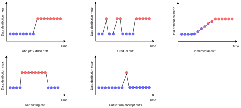
Figure 1. Different patterns of occurring concept drift in comparison with the outlier pattern.

Regarding where the shift takes place, we can distinguish input features to the corresponding learning model, and targets of the prediction space of the model. Based on this, we can distinguish three important types of concept drift.

First, covariate drift arises when the distribution of attributes changes over time, and the conditional distribution of the target with respect to the attributes remains invariant (Gama et al., 2014; Webb et al., 2016). For instance, take business systems that use socio-economic factors (attributes) for user classification (the class of users is the target here). Shifting the demography of the customer base (as part of attributes) during the time changes the probability of demographic factors (Webb et al., 2016). This type of drift can occur both in classification and regression tasks.

Second, target drift (also known as concept drift or class drift) arises when the conditional distribution of the target with respect to attributes changes over time, while the distribution of attributes remains unaffected (Gama et al., 2014; Webb et al., 2016). An example of this type of drift may occur in network intrusion detection (Žliobaitė et al., 2016). An abrupt usage pattern (usage metrics are attributes here) in the network can be an adversary behavior or a weekend activity (class labels are targets here) by normal users. In this case, we confront the same set of data attributes for the decision but with different classes (target) of meanings behind these scenarios that depend on the activity time (attributes). This type of drift can also occur in both types of prediction tasks, regression and classification.

Third, novel class appearance is a type of concept drift about emerging new classes in the target over time (Masud et al., 2010; Webb et al., 2016). Hence, for a new class, the probability of having any data with the new class in the target is zero before it appears. Over time the data with the new class emerges, and there is a positive probability of observing such data. Examples of this type of drift (Mustafa et al., 2017) are novel intrusions or attacks (as new targets) appearing in the security domain (Araujo, 2016; Araujo et al., 2014) and new physical activities (as new targets) in the monitoring stage of wearable devices (Reiss and Stricker, 2012). In contrast to covariate and target drifts, this type of drift can only occur in classification tasks.

2.2. Lifelong Machine Learning

Lifelong machine learning enables a machine-learning system to learn new tasks that were not predefined when the system was designed (Thrun and Mitchell, 1995). It mimics the learning processes of humans and animals that accumulate knowledge learned from earlier tasks and use it to learn new tasks and solve new problems. Technically, lifelong machine learning is a continuous learning process of a learner (Chen and Liu, 2018). Assume that at some point in time, the learner has performed a sequence of $n$ learning tasks, $\mathcal{T}_{1},\mathcal{T}_{2},\cdots,\mathcal{T}_{n}$, called the previous tasks, that have their corresponding data sets $\mathcal{D}_{1},\mathcal{D}_{2},\cdots,\mathcal{D}_{n}$. Tasks can be of different types and from different domains. When faced with task $\mathcal{T}_{n+1}$ (called the new or current task) with its data set $\mathcal{D}_{n+1}$, the learner can leverage past knowledge maintained in a knowledge-base to help learn task $\mathcal{T}_{n+1}$. The new task may be given by a stakeholder or it may be discovered automatically by the system. Lifelong machine learning aims to optimize the performance of the learner for the new task (or for an existing task by treating the rest of the tasks as previous tasks). After completing the learning task $\mathcal{T}_{n+1}$, the knowledge base is updated with the newly gained knowledge, e.g., using intermediate and final results obtained via learning. Updating the knowledge can involve checking consistency, reasoning, and mining meta-knowledge.

For example, consider a lifelong machine learning system for the never-ending language learner (Mitchell et al., 2018) (NELL in short). NELL aims to answer questions posed by users in natural language. To that end, it sifts the Web 24/7 extracting facts, e.g., “Paris is a city.” The system is equipped with a set of classifiers and deep learners to categorize nouns and phrases (e.g., “apple” can be classified as “Food” and “Company” falls under an ontology), and detecting relations (e.g., “served-with” in “tea is served with biscuits”). NELL can infer new beliefs from this extracted knowledge, and based on the recently collected web documents, NELL can expand relations between existing noun phrases or ontology. This expansion can be a change within existing ontological domains, e.g., politics or sociology, or be a new domain like internet-of-things. Hence, the expansion causes an emerging task like classifying new noun phrases for the expanded part of the ontology.

Lifelong machine learning works together with different types of learners. In lifelong supervised learning, every learning task aims at recognizing a particular class or concept. For instance, in cumulative learning, identifying a new class or concept is used to build a new multi-class classifier for all the existing and new classes using the old classifier (Fei et al., 2016). Lifelong unsupervised learning focuses on topic modeling and lifelong information extraction, e.g., by mining knowledge from topics resulting from previous tasks to help generate better topics for new tasks (Wang et al., 2016). In lifelong semi-supervised learning, the learner enhances the number of relationships in its knowledge base by learning new facts, for instance, in the NELL system (Mitchell et al., 2018). Finally, in lifelong reinforcement learning each environment is treated as a task (Tanaka and Yamamura, 1998), or a continual-learning agent solves complex tasks by learning easy tasks first (Ring, 1997). Recently, lifelong learning has gained increasing attention, in particular for autonomous learning agents and robots based on neural networks (Parisi et al., 2019).

One of the challenges for lifelong machine learning is dealing with catastrophic forgetting, i.e., the loss of what was previously learned while learning new information, which may eventually lead to system failures (Nguyen et al., 2019). Another more common challenge is under-specification, i.e., a significant decrease of the performance of a learning model from training to deployment (or testing) (D’Amour et al., 2022). Promising approaches have been proposed, e.g., (Parisi et al., 2019) for catastrophic forgetting and (Ribeiro et al., 2020) for under-specification. Yet, more research is needed to transfer these techniques to real-world systems.

3. Problem of Drift of Adaptation Spaces

In this section, we introduce the setting of DeltaIoT that we use in this paper. Then we illustrate and elaborate on the problem of drift of adaptation spaces using a scenario of DeltaIoT.

3.1. DeltaIoT

DeltaIoT (Iftikhar et al., 2017) is an examplar in the domain of the Internet of Things that supports research in engineering self-adaptive systems, see e.g., (Weyns et al., 2018; Weyns and Iftikhar, 2022; Weyns et al., 2022; Edwards and Bencomo, 2018). Figure 2 shows the setup of the IoT network that we used for the research presented in this paper. The network consists of 16 battery-powered sensor motes that measure parameters in the environment and send the data via a wireless multi-hop network to a central gateway that connects with users at an application server that can use the data. Motes are equipped with various sensors, in particular RFID, temperature sensors, and motion sensors. The data collected by the motes can be used to monitor the campus area and take action when needed. The communication in the network is time-synchronized (Mills, 2017), i.e., the communication is organized in cycles (a number of minutes) where neighboring motes are allocated slots that they can use to send and receive messages over a wireless link as shown in the figure.

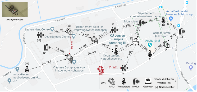
Figure 2. DeltaIoTv1.1 setup.

Two quality properties of interest in DeltaIoT are packet loss and energy consumption. In general, stakeholders want to keep both the packet loss and the energy consumption low. Yet, these quality properties are conflicting as using more energy will increase the signal strength and hence reduce packet loss. Furthermore, uncertainties have an impact on the qualities. We consider two types of uncertainties: the load of messages produced by motes, which varies depending on several aspects, including the number of humans sensed in the surroundings, and network interference caused by environmental circumstances, such as other networks and weather changes. Network interference affects the Signal-to-Noise Ratio (SNR) (Haenggi et al., 2009), which then influences the packet loss.

3.1.1. Self-adaptation

To mitigate the uncertainties and satisfy the goals of the stakeholders, we add a feedback loop at the gateway (i.e., a managing system) that monitors the IoT network (i.e., the managed system) and its environment and can adapt the network settings in each cycle.

The managing system can adapt two settings for each mote: (1) the power setting (a value in the range of 0 to 15), which will affect the SNR and hence the packet loss, and (2) the distribution of the messages along the outgoing network links (for motes with two links, a selection among the following options is possible: 0/100, 20/80, 40/60, 60/40, 80/20, 100/0). Because the power setting of each mote can be determined by the values of the sensed SNRs of it links, these values are determined in each cycle and used for all adaptation options. The adaptation options are then determined by the distribution of messaging for each mote with two links. Hence, the total number of possible adaptation options is equal to the possible configurations (0/100, 20/80, 40/60, 60/40, 80/20, 100/0) for 4 motes with two parent links (motes with the index of 7, 10, 11, and 12 in Figure 2). This creates in total $6^{4}=1296$ different configurations from which the managing system can select an option to adapt the system.

The left part of Figure 3 shows the estimated quality properties of the adaptation options in DeltaIoTv1.1 made by a verifier at runtime in one particular cycle, i.e., the adaptation space at that time. Each point shows the values of the estimated quality properties for one adaptation option. The right part of Figure 3 shows the distribution of the quality properties for all adaptation options over 180 adaptation cycles, i.e., a plot of all the adaptation spaces over 180 cycles.

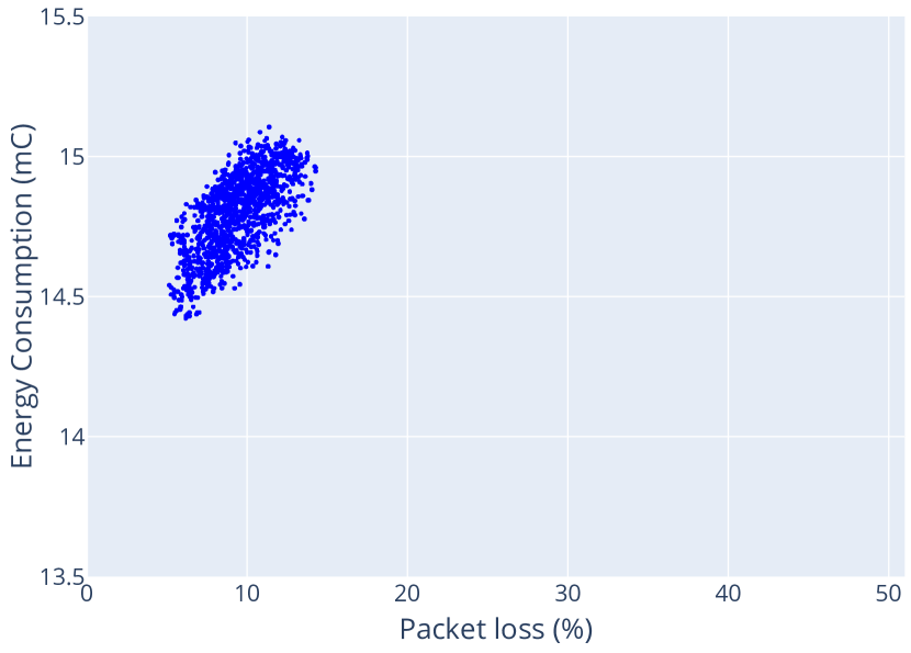
(a) Adaptation space in one cycle

(b) Adaptation spaces over 180 cycles

Figure 3. Left: the estimated quality properties of all the adaptation options of DeltaIoTv1.1 at one point in time. Right: the distribution of the quality properties for all adaptation options over 180 adaptation cycles.

3.1.2. Adaptation Goals

Figure 4 shows how the adaptation goals of the system are defined. Specifically, the adaptation goals are defined by the stakeholders as a ranking of regions in the plane of the quality properties of the system. This ranking is based on the preference order of the stakeholders. As an example, stakeholders may have a preference order $\langle$“less packet loss”, “less energy consumption”$\rangle$, which means stakeholders prefer less packet loss over less energy consumption. Technically, the overall goal of the system is defined based on a ranking over a set of classes characterized by a mixture of Gaussian distributions. This ranking then expresses the preference order of the stakeholders in terms of configurations of the system with particular quality properties. The stakeholder-defined classes (represented by contour elliptic curves) are created by fitting of Gaussian distributions over selected points (pairs of quality attributes) pertinent to each class. Each Gaussian distribution comprises three ellipsoids that show sigma, 2-sigma, and 3-sigma boundaries around the mean, from inside to outside, respectively. The preference order of the stakeholders over classes is determined by $m$ in $C_{i}^{(m)}$ for each class $i$. As each Gaussian distribution is defined over the infinity range (from $-\infty$ to $+\infty$), each point is assigned to every class (here, three classes) with a probability. Thus, the class corresponding to the highest probability is assigned to the data point, i.e., the adaptation option with its estimated qualities at that point in time. Note that the approach for lifelong self-adaptation we propose in this paper allows an operator to interact with the system to determine or adjust the ordering of the classes on behalf of the stakeholders.

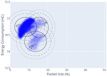
Figure 4. Stakeholder-defined classes (elliptic curves) created by fitting Gaussian distributions over selected points. The preference order of the stakeholders over these classes is determined by $m$ in $C_{i}^{(m)}$ for class $i$.

3.1.3. Learning-based Decision-making

The internal structure of the managing system shown in Figure 5 follows the Monitor-Analyse-Plan-Execute-Knowledge reference model (MAPE-K) (Kephart and Chess, 2003; Weyns et al., 2013). An operator initiates the learning model and the goal model (or interchangeably preference model) based on offline analysis of historical data before deploying the system. The learning model consists of a classification model of quality attributes. The goal model expresses the ordering of the classes in the classification model based on the preference order of the stakeholders (e.g., see Figure 4).

Figure 5. Learning-based self-adaptive system for DeltaIoT

The monitor component tracks the uncertainties (network interference of the wireless links and load of messages generated by the motes) and stores them in the knowledge component (steps 1 and 2). Then the analyzer component is triggered (step 3).

Algorithm 1 describes the analysis process (steps 4 to 8). The analyzer starts with reading the necessary data and models from the knowledge component (step 4, lines 3 and 4). Then, the analyzer uses the classifier to find an adaptation option with quality attributes that is classified as a member of a class with the highest possible ranking in the preference model. The selection of adaptation options happens randomly (by random shuffling of adaptation options in line 4). This option is then verified using the verifier (step 5, line 13). To that end, the verifier configures the parameterized quality models, one for each quality property, and initiates the verification (step 6). The parameters that are set are the actual uncertainties and the configuration of the adaptation option. We use in our work statistical model checking for the verification of quality models that are specified as parameterized stochastic timed automata, using Uppaal-SMC (David et al., 2015; Iftikhar and Weyns, 2014) (line 13). For details, we refer to (Weyns and Iftikhar, 2022; Iftikhar and Weyns, 2014). When the analyzer receives the verification results, i.e., the estimated qualities for the adaptation option (step 7), it uses the classifier to classify the data point based on the Gaussian Mixture Model (GMM) (line 15). This loop of verification and classification (steps 5 to 7) is repeated until the analyzer finds an adaptation option with a probability of being a member of the best class that is higher than a specific threshold (line 18). If no option of the best class is found (line 19), the loop is repeated for the next best-ranked class in the preference model (line 6), etc., until an option is found. Alternatively, the analysis loop ends when the number of detected outliers exceeds a predefined threshold (line 18). To ensure that each candidate adaptation option is verified only once (line 9 to 11), all verification and classification results are stored (we empirically determined data of the 1000 most recent cycles) in a dictionary of the knowledge (lines 14 and 16). Finally, the analyzer stores the verification and classification results in the knowledge component (step 8).

Algorithm 1 Analysis stage of the managing system

1:$\mathrm{PROB\_THR}\leftarrow 0.001$

2:$\mathrm{COUNTER\_THR}\leftarrow 10$

3:$\mathrm{uncs}\leftarrow\mathrm{K.tracked\_uncertainties[current\_cycle\_num]}$ $\triangleright$ SNRs + load of messages

4:$\mathrm{adpt\_opts}\leftarrow\mathrm{random\_shuffle}(\mathrm{K.adaptation\_options})$

5:$\mathrm{outlier\_counter}\leftarrow 0$

6:for each $\mathrm{p\_class\_index}$ in $\mathrm{preference\_model}.\mathrm{class\_rankings}$ do

7:     for each $\mathrm{option}$ in $\mathrm{adpt\_opts}$ do

8:         $\mathrm{key}\leftarrow(\mathrm{current\_cycle\_num},\mathrm{uncs},\mathrm{option})$

9:         if $\mathrm{key}$ exists in $\mathrm{K.results}$ then

10:              $\mathrm{packet\_loss},\mathrm{energy\_consumption}\leftarrow\mathrm{K.results}[\mathrm{key}].\mathrm{verification}$

11:              $\mathrm{class\_index},\mathrm{class\_prob}\leftarrow\mathrm{K.results}[\mathrm{key}].\mathrm{classification}$

12:         else

13:              $\mathrm{packet\_loss},\mathrm{energy\_consumption}\leftarrow$ $\mathrm{Verifier}.\mathrm{verify}(\mathrm{uncs},\mathrm{option})$

14:              $\mathrm{K.results}[\mathrm{key}].\mathrm{verification}\leftarrow(\mathrm{packet\_loss},\mathrm{energy\_consumption})$

15:              $\mathrm{class\_index},\mathrm{class\_prob}\leftarrow\mathrm{Classifier}.\mathrm{classify}(\mathrm{packet\_loss},\mathrm{energy\_consumption})$

16:              $\mathrm{K.results}[\mathrm{key}].\mathrm{classification}\leftarrow(\mathrm{class\_index},\mathrm{class\_prob})$

17:         end if

18:         if $\mathrm{class\_prob}>\mathrm{PROB\_THR}$ or $\mathrm{outlier\_counter}>\mathrm{COUNTER\_THR}$ then $\triangleright$ 3-sigma rule for detecting possible outliers

19:              if $\mathrm{class\_index}==\mathrm{p\_class\_index}$ then

20:                  return

21:              end if

22:         else

23:              $\mathrm{outlier\_counter}\leftarrow\mathrm{outlier\_counter}+1$

24:         end if

25:     end for

26:end for

After the analysis stage, the planner is triggered (step 9). The planner uses the analysis results (step 10) to select the best adaptation option, i.e., the option found by the analyzer in the highest possible ranked class according to the preference model of the stakeholders and generates a plan to adapt the managed system (step 11 in Figure 5). Finally, the executor is called (step 12).

The executor then reads the adaptation plan (step 13) and enacts the adaptation actions of this plan via the gateway to the motes of the IoT network (step 14).

3.2. Problem of Drift in Adaptation Spaces in DeltaIoT

The problem with a classification approach as exemplified by the approach we described for DeltaIoT is that the quality attributes of the adaptation options may change over time due to uncertainties. For example, during construction works, equipment or physical obstacles may increase the noise in the environment on a set of specific links. Consequently, the packet loss and energy consumption of the configurations that route packets via these links will be affected. As a result, the classes of adaptation options with particular values for quality attributes may disappear or new classes may appear over time that are not part of the initial classification model. We refer to this problem as a drift of adaptation spaces. This phenomenon may deteriorate the precision of the classification model and, hence, the reliability and quality of the system.

Figure 6 shows an instance of novel class appearance (cf. Figure 4) for the setup shown in Figure 2. This plot represents the distribution of the quality attributes of adaptation options over 300 cycles. The blue points are related to cycles 1 to 250, and the green points to cycles 250 to 300. Although the position of some of the adaptation options (with their quality attributes) after cycle 250 (green points) were derived from initially defined classes (distributions), clearly most of the adaptation options after cycle 250 are not part of these initial distributions and form a new class or classes.

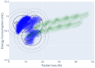
Figure 6. An example of novel class appearance in DeltaIot (cf. Figure 4). Blue points refer to the quality attributes for adaptation options over the initial 250 adaptation cycles. The green points refer to cycles 250 to 300.

To demonstrate the impact of this drift on the quality attributes of the IoT system, we compare the packet loss and energy consumption of the self-adaptive systems with a predefined classifier and with an ideal classifier (baseline) over 350 cycles. The ideal classifier used the verification results of all adaptation options in all cycles (determined offline as it takes three days to compute the ideal classifier). The stakeholders could then mark the different classes as shown in Figure 7. Note that the distribution of the population of each class obtained with the ideal classifier is close to its corresponding perfect Gaussian distribution, measured using sliced-Wasserstein distance (Bonneel et al., 2015) ($0.004\pm 1\mathrm{e}{-4}$, $0.003\pm 1\mathrm{e}{-4}$, $0.002\pm 2\mathrm{e}{-4}$, $0.008\pm 4\mathrm{e}{-4}$, and $0.009\pm 6\mathrm{e}{-4}$ — normalized to $[0\ldots 1]$ by the maximum distance between any two points of the data — for classes 1 to 5, respectively).

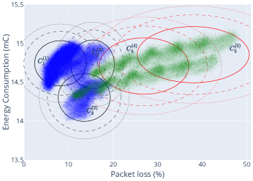
Figure 7. Ideal classifier with classes based on verification results of all adaptation options in all 350 adaptation cycles. The red elliptic curves (marked with $C^{4}_{4}$ and $C^{5}_{5}$) represent distributions of new data points that are not a member of any initially introduced classes (black elliptic curves) defined by the stakeholder.

We compare the two versions of the classifier with and without drift over 350 cycles for DeltaIoTv1.1 shown in Figure 2. Figure 8 shows the impact of the drift on the quality attributes of the system. For packet loss (8(a)), we observe an increase of the difference of the mean from $-0.75$ % (mean $9.91$ % for pre-defined classifier and $10.66$ % for the baseline) to $20.38$ % ($38.03$ % for pre-defined classifier and $17.65$ % for the baseline). For energy consumption (8(b)), we also observe an increase of the difference of the mean from a small difference of $-0.02$ mC ($14.64$ mC for pre-defined classifier and $14.66$ mC for the baseline) to $0.30$ mC ($14.83$ mC for pre-defined classifier and $14.53$ mC for the baseline). The results make clear that the impact on packet loss is dramatic (over 20% extra packet loss for the pre-defined classifier), while the effect on energy consumption is relatively small (0.30 mC on 14.83 mC is only 2$\%$ of the consumed energy).

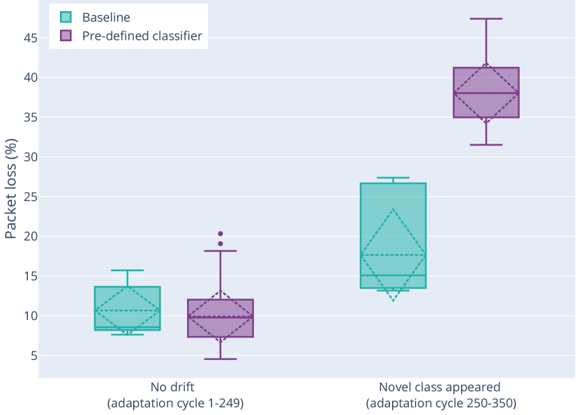
(a) Impact on packet loss.

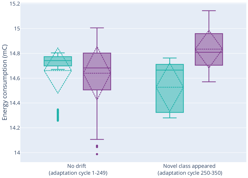
(b) Impact on energy consumption.

Figure 8. Impact of a shift of adaptation spaces (novel class appearance) on the quality attributes of the system for a predefined classifier compared to an ideal classifier (that serves as a baseline).

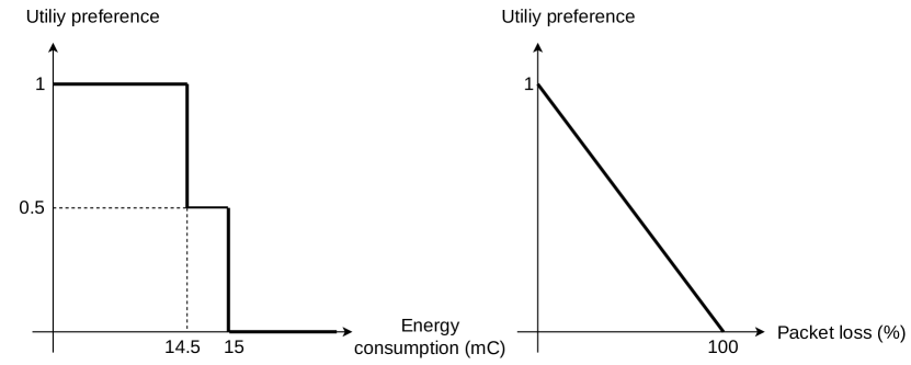
(a) The utility response curves.

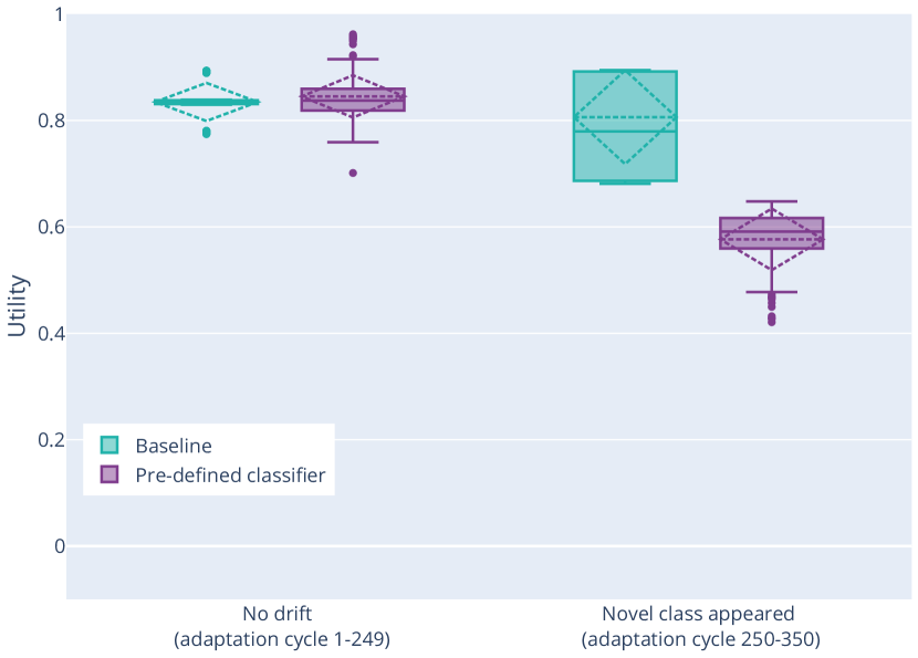
(b) Impact on the utility.

Figure 9. Left: utility response curves. Right: the impact of drift of adaptation spaces on the utility.

Since the impact on individual quality properties does not express the overall impact of the drift of adaptation spaces on the system, we also computed the utility of the system. We used the definition of utility as used in (Gheibi and Weyns, 2022) where the utility is defined as follows:

(1) $$U_{c}=0.2\cdot p_{ec}+0.8\cdot p_{pl}$$

with $p_{ec}$ and $p_{pl}$ the utility for energy consumption and packet loss respectively, and $0.2$ and $0.8$ the weights associated with the quality properties. The values of the utilities are determined based on the utility response curves shown in 9(a). These functions show that stakeholders give maximum preference to an energy consumption below 14.5 mC, medium preference to an energy consumption of 14.5 mC to 15 mC, and zero preference to energy consumption above 15 mC. On the other hand, the utility for packet loss decreases linearly from one to zero for packet losses from 0% to 100%. Figure 9(b) shows the results for the utility of the pre-defined classifier and the baseline split for the period before drift (cycles 1-249) and the period when drift of adaptation spaces occurs (cycles 250-350). The results show that the utility with the pre-defined classifier is close to the baseline for the period of no drift (mean 0.85 versus 0.83 respectively). Yet, for the period with drift, the utility for the pre-defined classifier drastically drops (mean 0.58 versus 0.81 for the baseline).

Comparing the individual quality attributes obtained with the two classifiers or using the utilities (derived from the quality attributes) provides useful insights into the effect of the drift of adaptation spaces on the system. Yet, these metrics offer either only a partial view of the effect of the drift of adaptation spaces (for individual quality attributes) or the interpretation is dependent on specific utility response curves and the weights of the utility function used to compute the utilities. Therefore, we introduced a new metric to measure of the drift of adaptation spaces that is based on the sum of the differences between the class ranking of the selected adaptation option in each adaptation cycle over a number of cycles for a pre-defined classifier and an ideal classifier (the baseline), respectively. Then, this sum is normalized by the sum of the maximum value of this difference in each adaptation cycle over the number of cycles. Note that this number of cycles is domain-specific and needs to be determined empirically. We call this metric Ranking Satisfaction Mean (RSM). The value for the RSM falls within the range of $[0,1]$. An RSM of zero indicates that the performance (the accuracy of the predictions to classify adaptation options correctly according to the class ranking defined by the stakeholders) obtained with a given classifier is equal to the performance of an ideal classifier. An RSM of $1$ represents the worst performance of a given classifier compared to an ideal classifier, i.e., the classifier classifies the options such that based on the ranking of the classes none of the classified options are in the correct class and the assigned class is the furthest class to the correct class based on the ranking. Formally, RSM is defined as follows:

Definition 3.0 (Ranking Satisfaction Mean (RSM)).

Take a given classifier $R$ and an ideal classifier $R^{*}$ (here GMM classifiers) and a set of ranked classes $C_{1}^{*(i_{1})},C_{2}^{*(i_{2})},\ldots,C_{m}^{*(i_{m})}$ ($\langle i_{1},i_{2},\ldots,i_{m}\rangle$ is a permutation of $\langle 1,2,\ldots,m\rangle$, ranking over classes $C_{1}^{*}$ to $C_{m}^{*}$). Also, suppose that ranks of selected adaptation options based on each of these classifiers, $R$ and $R^{*}$, employed by a managing system for $n$ adaptation cycles are respectively denoted by $r=\langle r_{1},r_{2},\ldots,r_{n}\rangle$ and $r^{*}=\langle r^{*}_{1},r^{*}_{2},\ldots,r^{*}_{n}\rangle$ ($r_{i},r^{*}_{i}\in\{1,2,\ldots,m\}$ for all $i$ from $1$ to $m$). The RSM of $r$ compared to $r^{*}$ is then defined as follows:

(2) $$\mathrm{\textit{RSM}}_{r^{*}}(r)=\frac{1}{n\times(m-1)}\sum_{i=1}^{n}\left(r_{i}-r^{*}_{i}\right)$$

Figure 10 shows the impact of the drift of adaptation spaces (novel class appearance) on the RSM, for every 10 adaptation cycles (i.e., $n=10$) (the drift is illustrated in Figure 6). The mean of RSM value remarkably increases from $0.002$ without drift to $0.543$ with drift. The results show that the performance of the pre-defined classifier before the drift occurs is quite close to that of the ideal classifier (baseline). However, once the drift occurs and novel classes appear, the performance of the pre-defined classifier drops significantly as demonstrated by the increased RSM.

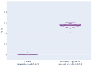
Figure 10. The impact of drift of adaptation spaces on RSM.

Based on Figures 8, 9 and 10, we can conclude that drift of adaptation spaces (novel class appearance) in learning-based self-adaptive systems can hinder the system from reaching its adaptation goals and may drastically reduce the level of satisfaction of the stakeholders.

4. Lifelong Self-Adaptation to Deal with Shift of Adaptation Spaces

We now introduce the novel approach of lifelong self-adaptation. We start with a general approach of lifelong self-adaptation that enables learning-based self-adaptive systems to deal with new learning tasks during operation. Then we instantiate the general architecture for the problem of learning-based self-adaptive systems that need to deal with shifts in adaptation spaces.

4.1. General Architecture of Lifelong Self-Adaptation

We start with assumptions and requirements for lifelong self-adaptation. Then we present the architecture of a lifelong self-adaptive system and we explain how it deals with new tasks.

4.1.1. Assumptions for Lifelong Self-Adaptation

The assumptions that underlie lifelong self-adaptation are:

• The self-adaptive system comprises a managed system that realizes the domain goals for users in the environment and a managing system that interacts with the managed system to realize the adaptation goals;

• The managing system is equipped with a learner that supports the realization of self-adaptation;

• The self-adaptive system provides the probes to collect the data that is required for realizing lifelong self-adaptation; this includes an interface to the managing system and the environment, and an operator to support the lifelong self-adaptation process if needed;

• The managing system provides the necessary interface to adapt the learning models.

In addition, we assume that the (target) data relevant to new class appearances comprises a mixture of Gaussian distributions. Lastly, we only consider new learning tasks that require an evolution of the learning models; runtime evolution of the software of the managed or managing system is out of the scope of the research presented in this paper.

4.1.2. Requirements for Lifelong Self-Adaptation

A lifelong self-adaptive system should:

1. Provide the means to collect and manage the data that is required to deal with new tasks;

2. Be able to discover new tasks based on the collected data;

3. Be able to determine the required evolution of the learning models to deal with the new tasks;

4. Evolve the learning models such that they can deal with the new tasks.

4.1.3. Architecture of Lifelong Self-Adaptive Systems

Figure 11 shows the architecture of a lifelong self-adaptive system. We explain the role of each component and the flow of activities among them.

Figure 11. The architecture of a lifelong self-adaptive system

Managed System

Interacts with the users to realize the domain goals of the system.

Managing System

Monitors the managed system and environment and executes adaptation actions on the managed system to realize the adaptation goals. The managing system comprises the MAPE components that share knowledge. The MAPE functions are supported by a learner, which primary aim is to solve a learning problem (Gheibi et al., 2020). Such problems can range from keeping runtime models up-to-date to reducing large adaptation spaces and updating adaptation rules or policies. The managing system may interact with an operator for input (explained below).

Lifelong Learning Loop

Adds a meta-layer on top of the managing system, leveraging the principles of lifelong machine learning. This layer tracks the layers beneath and when it detects a new learning task, it will evolve the learning model(s) of the learner of the managing system accordingly. We elaborate now on the components of the lifelong learning loop and their interactions.

Knowledge Manager

Collects and stores all knowledge that is relevant to the learning tasks of the learner of the managing system (realizing requirement R1). In each adaptation cycle, the knowledge manager collects a knowledge triplet: $k_{i}$ = $\langle$input_i, state_i, output_i$\rangle$. Input is the properties and uncertainties of the system and its environment (activity 1.1.1). State refers to data of the managing system relevant to the learning tasks, e.g., settings of the learner (1.1.2). Output refers to the actions applied by the managing system to the managed system (1.1.3). Sets of knowledge triplets are labeled with tasks $t_{i}$, i.e., $\langle$t_i, $\{$k_u, k_v, k_w$\}$$\rangle$, a responsibility of the task manager. The labeled triplets are stored in the repository with knowledge tasks. Depending on the type of learning tasks at hand, some parts of the knowledge triples may not be required by the lifelong learning loop.

Depending on the problem, the knowledge manager may reason about new knowledge, mine the knowledge, and extract (or update) meta-knowledge, such as a cache or an ontology (1.2). The meta-knowledge can be used by the other components of the lifelong learning loop to enhance their performance. The knowledge manager may synthesize parts of the knowledge to manage the amount of stored knowledge (e.g., outdated or redundant tuples may be marked or removed).

Task manager

Is responsible for detecting new learning tasks (realizing R2). The task manager periodically retrieves new knowledge triplets from the knowledge manager (activity 2.1). The duration of a period is problem-specific and can be one or more adaptation cycles of the managing system. The task manager then identifies task labels for the retrieved knowledge triplets. A triplet can be assigned the label of an existing task or a new task. Each new task label represents a (statistically) significant change in the data of the knowledge triplets, e.g., a significant change in the distribution of the data observed from the environment and managed system. Hence, a knowledge triplet can be associated with multiple task labels, depending on the overlap of their corresponding data (distributions). The task manager then returns the knowledge triplets with the assigned task labels to the knowledge manager, which updates the knowledge accordingly (2.2). Finally, the task manager informs the knowledge-based learner about the new tasks (2.3).

Knowledge-based learner

Decides how to evolve the learning models of the learner of the managing system based on the collected knowledge and associated tasks (realizing R3), and then enacts the evolution of the learning models (realizing R4). To collect the knowledge it needs for the detected learning tasks, the knowledge-based learner queries the task-based knowledge miner (3.1) that returns task-specific data (3.2); the working of the task-based knowledge miner is explained below. The knowledge-based learner then uses the collected data to evolve the learning models of the managing system (3.3). This evolution is problem-specific and depends on the type of learner at hand, e.g., tuning or retraining the learning models for existing tasks, or generating and training new learning models for newly detected tasks. The knowledge-based learner then updates the learning models (3.4). Optionally, the managing system may show these updates to the operator who may provide feedback (3.5.1 and 3.5.2), for instance ordering a set of existing and newly detected tasks (e.g., the case where learning tasks correspond to classes that are used by a classifier).

Task-based knowledge miner

Is responsible for collecting the data that is required for evolving the learning models for the given learning task by the knowledge-based learner (supports realizing R3). As a basis, the task-based knowledge miner retrieves the knowledge triplets associated with the given task from the knowledge tasks repository, possibly exploiting meta-knowledge, such as a cache (3.1.1). Additionally, the task-based knowledge miner can mine the knowledge repositories of the knowledge manager, e.g., to retrieve knowledge of learning tasks that are related to the task requested by the knowledge-based learner. Optionally, the task-based knowledge miner may collect knowledge from stakeholders, for instance, to confirm or modify the labels of knowledge triplets or newly detected tasks (activities 3.1.2.1 and 3.1.2.2). Finally, the miner uses new knowledge to update the knowledge maintained in the repositories by the knowledge manager (3.1.3), e.g., it may update meta-knowledge about related tasks or add data to the knowledge provided by stakeholders.

Interplay between the knowledge-based learner and the learner of the managing system

Since both the knowledge-based learner and the learner of the managing system act upon the learning model as shown in Figure 12, it is important to ensure that this interaction occurs in a consistent manner.

Figure 12. Interplay between the knowledge-based learner and the learner of the managing system

Changes applied to learning models can be categorized into two main types: parametric changes and structural changes. Parametric changes pertain to adjustments made to the parameters of the current learning models. This may involve incrementally modifying the parameters of the learning model, like adjusting the vectors of a support vector machine based on newly observed training data or retraining the model with a new set of training data. On the other hand, structural changes involve alterations to the structure of learning models, such as adjusting the number of neurons or layers in a neural network, or even replacing an existing learning model with a new type of model, such as substituting a support vector machine with a Hoeffding adaptive tree.

Lifelong self-adaptation supports two approaches for changing the learning models: (1) the learner in the managing system uses the learning models to perform the learning tasks; the lifelong learning loop can apply structural changes to the learning models, and (2) the learner in the managing system performs the learning task and can apply parametric changes to the learning models (dotted lines in Figure 12); the lifelong learning loop can apply structural changes to the learning models. The instance of architecture for lifelong self-adaptation used in the evaluation case in this paper applies approach (1). The instances of the architecture used in the cases of (Gheibi and Weyns, 2022) (that are summarised in Section 4.1.4 below) apply approach (2).

By properly allocating the concerns, i.e., applying the learning task and parametric changes of the learning models allocated to the managing system, and structural changes of the learning models allocated to the lifelong learner, we can optimally deal with potential conflicts when changing the learning models. Since there are only structural changes in the learning models for approach (1), no conflicts can occur (under the condition that the learning models are evolved atomically, i.e., without the interference of performing learning tasks by the learner of the managing system). For approach (2), a conflict may occur if the training data used by the managing system to update the learning models contradicts the data mined by the task-based knowledge miner to evolve the learning models. This may degrade the performance of the evolved learning models due to drift in the training data. To avoid this issue, the learner of the managing system should only update the evolved learning models based on new data that is observed between two consecutive cycles of the lifelong learning loop (to be certain that this data pertains to the current task of the system). Hereby, it is important to note that the cycle time of the lifelong learner is often multiple times longer than the cycle time of the learner of the managing system.

4.1.4. Lifelong Self-Adaptation to Deal with Sudden and Incremental Covariate Drift

In (Gheibi and Weyns, 2022), we instantiated the general architecture for lifelong self-adaptive systems (shown in Figure 11) for two types of drift: recurrent sudden and incremental covariate drift. We briefly summarise these two instances of the general architecture here, for further details we refer the interested reader to (Gheibi and Weyns, 2022).

For the case of recurrent sudden covariate drift, we instantiated the architecture of lifelong self-adaptive systems for DeltaIoT. Recurrent sudden covariate drift occurs when the distributions of input data that are used by the managing system suddenly change and at some point may return to the same state, for instance, due to machinery that periodically produces noise patterns affecting the signal-to-noise ratio of the network links in the IoT network. In this instance, the underlying managing system predicts the quality attributes of the adaptation options either using a stochastic gradient descent (SGD) regressor (Saad, 1998) or by switching between an SGD and a Hoeffding Adaptive Tree (Bifet and Gavaldà, 2009). The task manager of the lifelong learning loop in this instance uses auto-encoders (Jaworski et al., 2020; Yang et al., 2021; Andresini et al., 2021) to detect new tasks (i.e., new distribution of features in the input data). The knowledge-based learner optimizes the hyper-parameters of each learning model using a Bayesian optimizer and then trains the best model based on the collected training data. The task-based knowledge miner simply fetches newly collected knowledge from the knowledge manager. Hence, the lifelong learning loop operates without human intervention. When the learning models are trained, they are updated in the knowledge repository of the managing system.

For the case of incremental covariate drift, we instantiated the architecture of lifelong self-adaptive systems for a gas delivery station (Vergara et al., 2012). The gas station composes substances to produce different types of gas that are routed to specific users. When composing the gas, there is uncertainty about the type of gas that is produced. To mitigate this uncertainty, a feedback loop collects data from sensors at the gas tank and uses a classifier, a multi-class support vector machine (SVC) (Angulo et al., 2003), to predict the gas type. The valves for gas delivery are then set such that the gas is routed to the right users. Similar to the first instance, the task manager of the lifelong learning loop uses auto-encoders to detect new tasks that emerge from drift in the measurements of gas sensors over time. The knowledge-based learner also uses a Bayesian optimizer to tune the hyper-parameters of the SVC learning model and train the most optimal model using the acquired training data. In contrast to the previous instance, the task-based knowledge miner requires feedback from the stakeholder on the labeling of some newly collected data (because data labeling here needs some chemical tests by the stakeholder). The aim is to minimize the interaction with the stakeholder by minimizing the number of required data labeling using active learning. After completing the training, the knowledge repository of the managing system is updated with the latest model.

In these two instances concept drift occurs in input features of the learning model of the learner. In novel class appearance, on the other hand, the type of concept drift we study in this paper, drift occurs in the target of the learner, i.e., the prediction space of the learning model.

4.2. Lifelong Self-Adaptation to Deal with Shift of Adaptation Spaces

We now instantiate the general architecture for lifelong self-adaptation to tackle the problem of shift in adaptation spaces in learning-based self-adaptive systems. Figure 13 shows the instantiated architecture illustrated for DeltaIoT (the managed system). We elaborate on the high-level components and their interactions that together solve the problem of shift of adaptation spaces.

Knowledge Manager (KM)

The knowledge manager starts the lifelong learning loop in the $i$-th adaptation cycle by collecting the state of the classifier from the managing system, denoted by $\mathrm{state}_{i}$ (link 1.1). This state includes the verification and classification results, the classification model of the learner on the quality attributes, and the preference model on classes (goal model). The knowledge manager stores and maintains a history of knowledge over a given window in a cache (link 1.2 in Figure 13). Note that this instantiation of the architecture of lifelong self-adaptation does not use the input and the output of the knowledge triplet, see the explanation of the general architecture (links 1.1.1 and 1.1.3 in Figure 13 of the general architecture are not required in the instantated architecture, and link 1.1.2 the general architecture is represented as link 1.1).

Figure 13. Architecture of lifelong self-adaptation to deal with drift of adaptation spaces illustrated for DeltaIoT.

Task Manager

A “task” in the general architecture corresponds to a “class” in the instantiated architecture, expressed by mixed Gaussian distributions on quality attributes. Hence, the task manager is responsible for detecting (new) classes based on the Gaussian Mixture Model (GMM) previously defined by the stakeholders (stored in the knowledge of states collected by the knowledge manager). Algorithm 2 describes the detection algorithm in detail.

The task manager starts with collecting the required knowledge of states (link 2.1 in Figure 13 and lines 4 and 5 in the algorithm), i.e., recently observed states of the classifier, including the last goal model. Then, using the classification model and the 3-sigma method (Czitrom and Spagon, 1997), the algorithm finds out which pairs of verified quality attributes in the collected states are characterized as data not belonging to existing classes, i.e., out-of-classes-attributes (lines 6 to 12). The algorithm then computes the percentage out-of-classes-attributes of the total number of considered quality attributes in the collected states (line 13) and compares this with a threshold (line 14). If the percentage out-of-classes-attributes does not cross the threshold, the algorithm will terminate (do nothing, line 15). However, if the threshold is crossed, some new classes have emerged, and the algorithm fits a GMM over the data (lines 17 and 18). The first step to fitting a GMM is determining the number of classes (or components) (line 17). To that end, the algorithm uses the Bayesian Information Criterion curve (Schwarz, 1978; Konishi and Kitagawa, 2008) (BIC curve) for the different number of classes. Afterward, the algorithm employs a common method, called Kneedle algorithm (Satopaa et al., 2011), to find an elbow (or a knee) in this curve to specify a Pareto-optimal number of classes. For example, Figure 14 represents a BIC curve with an indicated elbow/knee point that occurs at 2 components, i.e., the distribution of the quality attribute pairs (during the specified adaptation cycles) can be reasonably expressed as the sum of two Gaussian distributions, meaning two classes. After specifying the number of classes, the algorithm uses the expectation-maximization algorithm to fit a GMM over the out-of-classes-attributes (line 18). Then a new classification model is constructed by integrating the last classification model of the system and the newly detected one (line 19). Finally, the task labels of all collected states are updated based on classification results obtained by applying the new classification model to the quality attributes related to the state (link 2.2 in Figure 13 and lines 20 to 23 in the algorithm). This concludes the detection algorithm of the task manager. When the task manager detects some new class(es) it triggers the knowledge-based learner (link 2.3 in Figure 13).

Algorithm 2 Detection of (new) classes in quality attributes (in task manager)

1:$\mathrm{OUT\_OF\_CLASS\_PERCENT\_THR}\leftarrow 20$

2:$\mathrm{ADAPT\_CYCLE}\leftarrow 10$

3:$\mathrm{out\_of\_class\_attrs}\leftarrow[]$

4:$\mathrm{states}\leftarrow\mathrm{KM}.\mathrm{Knowledge}[-\mathrm{ADAPT\_CYCLE}:]$ $\triangleright$ collect recent states of adaptation cycles

5:$\mathrm{classification\_model}\leftarrow\mathrm{states[end]}.\mathrm{Classfication\_Model}$

6:for each $\mathrm{state}\in\mathrm{states}$ do

7:     for each $\mathrm{attr}\in\mathrm{state}.\mathrm{quality\_attributes}$  do

8:         if $\mathrm{classification\_model}.\mathrm{is\_out\_of\_class}(\mathrm{attr})$ then $\triangleright$ using 3-sigma method

9:              $\mathrm{out\_of\_class\_attrs}.\mathrm{append}(attr)$

10:         end if

11:     end for

12:end for

13:$\mathrm{out\_of\_class\_percent}\leftarrow{100\times|\mathrm{out\_of\_class\_attrs}|}/\left({\sum_{\mathrm{state}\in\mathrm{states}}|\mathrm{state}.\mathrm{quality\_attributes}|}\right)$

14:if $\mathrm{out\_of\_class\_percent}<\mathrm{OUT\_OF\_CLASS\_PERCENT\_THR}$ then

15:     $\triangleright$ do nothing

16:else$\triangleright$ new class(es) detected

17:     $\mathrm{component\_num}\leftarrow\mathrm{find\_component\_num}(\mathrm{out\_of\_class\_attrs})$

18:     $\mathrm{new\_model}\leftarrow\mathrm{fit\_GMM\_model}(\mathrm{out\_of\_class\_attrs},\mathrm{component\_num})$ $\triangleright$ using EM

19:     $\mathrm{classification\_model}\leftarrow\mathrm{classification\_model}+\mathrm{new\_model}$ $\triangleright$ GMM model

20:     for each $\mathrm{state}\in\mathrm{KM}.\mathrm{Knowledge}[-\mathrm{ADAPT\_CYCLE}:]$ do $\triangleright$ update task labels

21:         $\mathrm{task\_labels}\leftarrow\mathrm{classification\_model}.\mathrm{classify}(\mathrm{state.Quality\_Attributes})$

22:         $\mathrm{KM}.\mathrm{Task\_Label}[\mathrm{state}]\leftarrow\mathrm{task\_labels}$

23:     end for

24:end if

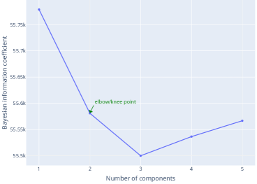
Figure 14. A BIC curve (based on the different number of components) for the quality attribute pairs corresponding to all adaptation options in adaptation cycles 151 to 160.

Knowledge-Based Learner

When the knowledge-based learner is triggered by the task manager, it queries the task-based knowledge miner (link 3.1 in Figure 13) to collect knowledge connected to the newly detected class(es) (link 3.2). The knowledge-based learner then fits a GMM on the gathered data (verification results) and integrates with the last state of the GMM classification model of the system (link 3.3). Finally, the knowledge-based learner updates the goal classification model in the managing system with the created GMM (link 3.4). We elaborate on the interaction with the operator below (i.e., links 3.5.1 and 3.5.1).

Task-Based Knowledge Miner

Based on the query from the knowledge-based learner (link 3.1), the task-based knowledge miner collects newly observed and labeled knowledge of states from the knowledge manager (link 3.1.1). Then, similar to Algorithm 2, the task-based knowledge miner initiates a GMM classification model on the gathered data and combines it with the last classification model of the system (from the last observed state). The task-based knowledge miner then provides the operator with a visual representation of this classification model (link 3.1.2.1). The operator can then give feedback on the proposed classification model (link 3.1.2.2). Figure 15 illustrates the different steps of the interaction of the operator with the task-based knowledge miner via a GUI.

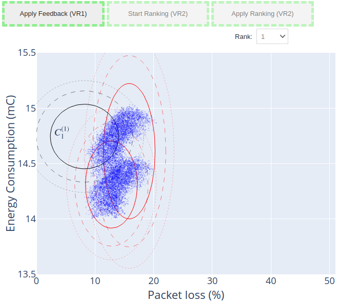
(a) Initial classification shown to the operator.

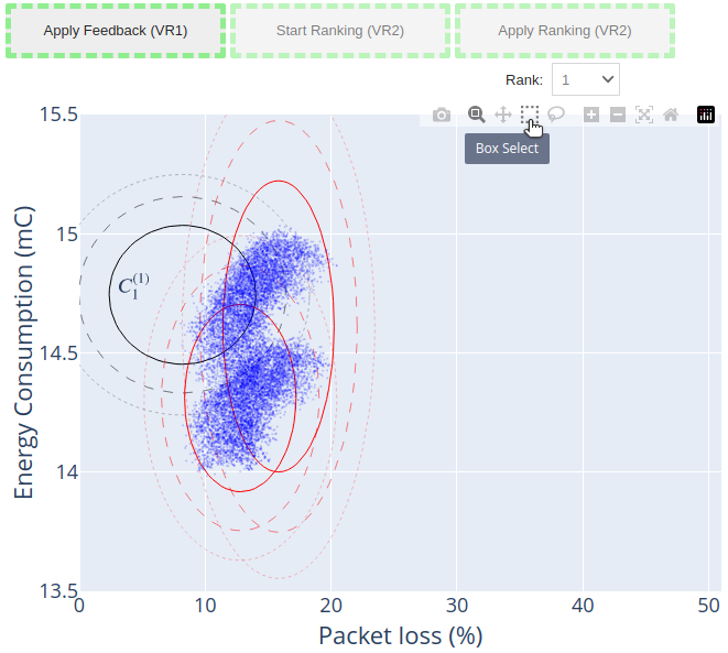
(b) The operator select the “Box Selection” option.

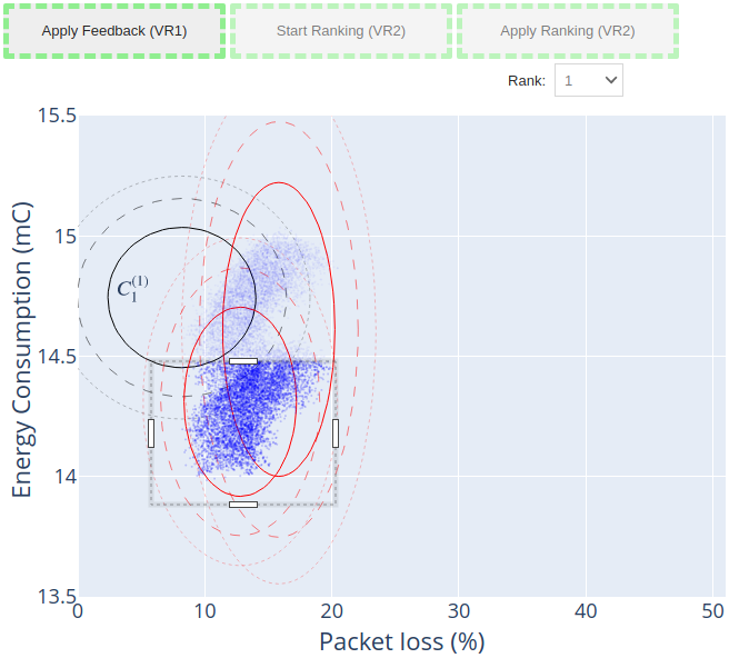
(c) The operator marks a reasonable area of a new class and confirms by clicking “Apply Feedback.”

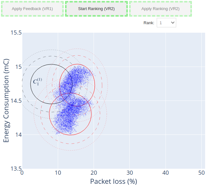
(d) The operator starts ranking the new classification by clicking “Start Ranking” using the “Rank” option.

Figure 15. Illustration of the interaction of the operator with the task-based knowledge miner via a GUI.

Figure 15(a) shows a visualization of the classification model using the verified quality attributes in the specified adaptation cycles (indicated by blue points). The black elliptic curve shows a previously detected class. The red elliptic curves show distributions of newly detected classes based on recently observed quality attributes of adaptation options. In this example, there is a visual distinction between two new classes (groups of quality attributes mapping to adaptation options) based on energy consumption. However, the GMM has not represented this distinction well. As the stakeholders may desire less energy consumption, the operator uses a box selector to separate the two groups by enclosing one of the groups (the other group is outside of it) (Figure 15(b) and Figure 15(c)). By clicking the “Apply Feedback” button the operator will provide the feedback to the task-based knowledge miner (link 3.1.2.2 in Figure 13). The task-based knowledge miner then applies the feedback (fitting a new GMM on the newly collected data based on the feedback) and shows the new classification to the stakeholder (Figure 15(d)). Finally, the task-based knowledge miner updates the labels of the collected data using the feedback from the operator (link 3.1.3) and returns the updated knowledge to the knowledge-based learner responding to the query (link 3.2).

We now come back on the interaction of the operator with the managing system (links 3.5.1 and 3.5.2). When new classes are detected, the operator should update the ranking of the classes in the preference model (including previously and newly detected classes). This is illustrated in Figure 16. The operator starts the ranking process by clicking the “Start Ranking” button in the GUI (Figure 16(a)). The managing system then shows the preference model to the operator (link 3.5.1). During the ranking process (Figure16(a) to Figure 16(c)), one class is highlighted (with purple color) in each step that needs to be ranked. To that end, the operator selects the desirable rank for the class from the menu (e.g., the operator selects class 3 for the highlighted class in Figure 16(b)) and assigns the rank by clicking the “Apply Ranking” button. After ordering all classes, the final total ranking of the classification model is shown to the stakeholder (Figure 16(d)) and this ranking is applied to the preference model of the managed system (link 3.1.2.3 in Figure 13).

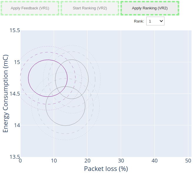
(a) The operator can rank the (purple) marked class.

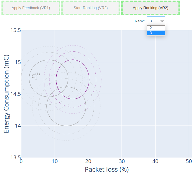
(b) The operator can rank the next marked class.
.

(c) The operator can rank the last marked class.

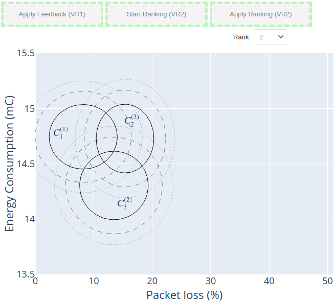
(d) Total ordering of classes that the task-based knowledge can use to update the preference model.

Figure 16. Illustration of the interaction of the operator to update the preference model.

Tasks of the learners

Recall that the adaptation goals are defined by the stakeholders as a ranking of regions in the plane of the quality properties of the system. In our solution, we assume that the borders of previously identified classes remain static over time. The knowledge-based learner then fits the optimal mixture of Gaussian distributions on the newly detected data and incrementally incorporates them into the existing mixture of Gaussian models in the managing system (i.e., a structural change). Hence, the learner in the managing system solely performs queries to classify data points and does not perform any parametric change on the learning model over time. Additionally, as stated in the assumptions of the approach, the knowledge-based learner uses the same interface definition for the GMM as the learner of the managing system.

5. Evaluation

We evaluate now lifelong self-adaptation to deal with a drift of adaptation spaces. To that end, we use the DeltaIoT simulator with a setup of 16 motes as explained in Section 3.1. We applied multiple scenarios with novel class appearance over 350 adaptation cycles that represent three days of wall clock time. The evaluation was done on a computer with an i7-3770 @ 3.40GHz processor and 16GB RAM. A replication package is available on the project website (Gheibi and Weyns, 2024). The remainder of this section starts with a description of the evaluation goals. Then we explain the evaluation scenarios we use. Next, we present the evaluation results. Finally, we discuss threats to validity.

5.1. Evaluation Goals

To validate the approach of lifelong self-adaptation for drift of adaptation spaces in answer to the research question, we study to following evaluation questions:

• How effective is lifelong self-adaptation in dealing with drift of adaptation spaces?

• How robust is the approach to changing the appearance order of classes and different preference orders of the stakeholders?

• How effective is the feedback of the operator in dealing with drift of adaptation spaces?

To answer EQ1, we measured the values of the quality attributes over all adaptation cycles and based on these results we computed the utility and the RSM (as defined in Section 3.2) before and after novel class(es) appear. We performed the measurements and computations for four approaches: (i) the managing system equipped with an ideal classifier that uses a correct ranking of classes, we refer to this approach as the baseline; (ii) the managing system equipped with a pre-defined classifier with ML2ASR (Quin et al., 2022); this is a representative state-of-the-art approach of learning-based self-adaptation that applies adaptation space reduction, (iii) a pre-defined classifier with lifelong self-adaptation (no operator feedback), and (iv) an evolving classifier with lifelong self-adaptation with operator feedback. All classifiers rely on mixed Gaussian distributions on quality attributes (GMM). For approach (ii), we implemented a self-adaptation approach that leverages Machine Learning to Adaptation Space Reduction (ML2ASR) (Quin et al., 2022). This approach uses a regressor to predict quality attributes in the analysis stage and then uses the prediction result to rank and select a subset of the adaptation options for verification, i.e., the approach verifies those adaptation options that are classified as a higher-ranking class as in Algorithm 1. Note that to the best of our knowledge, there are no competing approaches for dealing with the novel class appearance in the context of self-adaptive systems that interact with an operator on behalf of stakeholders to order classes. Hence, we compared the proposed approach with a perfect baseline and a related state-of-the-art approach that uses learning to predict quality attributes of the adaptation options at runtime.

To answer the evaluation questions EQ2 and EQ3 we applied the evaluations of EQ1 for multiple scenarios that combined different preference orders of stakeholders and different orders of emerging classes with and without feedback from an operator. For questions EQ2 and EQ3 we focused on the period of new appearance of classes within each scenario.

Before explaining the evaluation scenarios, we acknowledge that we evaluated the instantiated architecture of lifelong self-adaptation for dealing with a novel class appearance in only one domain. Finding and evaluating solutions beyond one domain goes beyond the scope of the research presented in this paper and offers opportunities for future research. We anticipate that the instance of the architecture presented in this paper may lay a foundation for such future studies.

5.2. Evaluation Scenarios

Table 1 shows the different scenarios that we use for the evaluation comprising three factors.

Table 1. Evaluation scenarios

Preference order of stakeholders	Classes appearance order	Operator feedback
$\langle$“less packet loss”, “less energy consumption”$\rangle$, $\langle$“less energy consumption”, “less packet loss” $\rangle$	$\langle$(B), R, G$\rangle$, $\langle$(B), G, R$\rangle$, $\langle$(R), B, G$\rangle$, $\langle$(R), G, B$\rangle$, $\langle$(B, R), G$\rangle$, $\langle$(B, G), R$\rangle$,	$\langle$active$\rangle$, $\langle$inactive$\rangle$

The first factor (left column of Table 1) shows the two options for the preference order of the stakeholders. This factor allows us to evaluate the robustness against different preference orders of the stakeholder (EQ2) of the lifelong self-adaptation approach.

The second factor (middle column of Table 1) shows six options for the appearance order of classes over time. Each character, $B$, $R$, and $G$, refers to a group of classes in the quality attribute plane, as illustrated in Figure 17. The order expresses the appearances of groups over time. For instance, $\langle$(B), R, G$\rangle$ means that first, the group of classes marked with $B$ appears, then the group $R$ appears, and finally group $G$ appears. Figure 18 illustrates this scenario. The groups of classes marked between round brackets are known before deployment (order-invariant) and can be used for training the learners. The classifiers were trained for a number of cycles (between 40 and 180 cycles) depending on the appearance of new classes in each scenario. Since the order of appearance of classes may affect the effectiveness of lifelong self-adaptation, we analyzed the different scenarios to validate the robustness to changing the appearance order of classes (EQ2) of the proposed approach.

Figure 17. Groups of classes in the quality attribute panel where adaptation options appear.

(a) Adaptation cycle 1-40

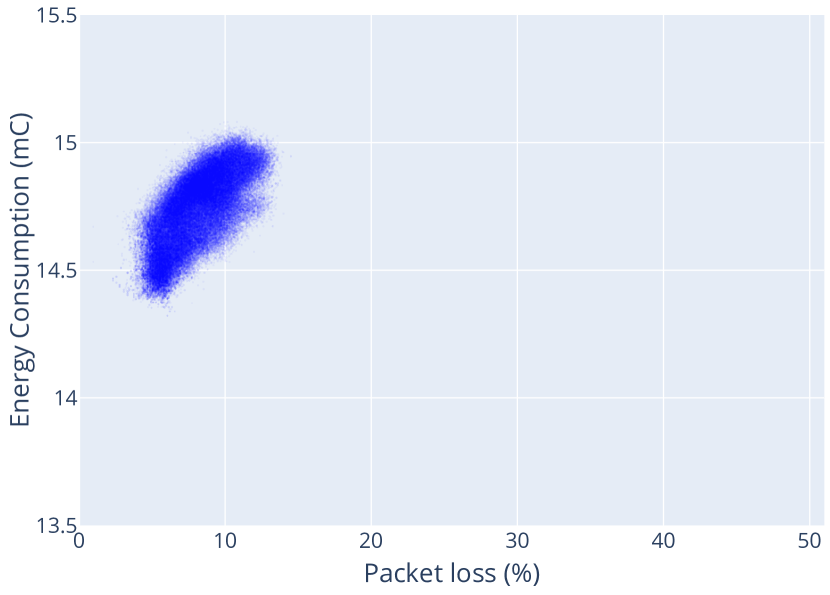
(b) Adaptation cycle 41-140

(c) Adaptation cycle 141-160

(d) Adaptation cycle 161-240

(e) Adaptation cycle 241-260

(f) Adaptation cycle 261-350

Figure 18. Adaptation spaces for the base scenario illustrating novel class appearance over time.

Finally, the third factor (right column of Table 1) expresses whether the operator is actively involved in the self-adaptation process (active) or not (inactive). This involvement refers to the activities related to links 3.1.2.1, 3.1.2.2, 3.5.1, and 3.5.2 in Figure 13. This factor allows us to evaluate the effectiveness of feedback from the operator in dealing with a drift of adaptation spaces (EQ3).

By combining the three factors (preference order of stakeholders, appearance order of classes, and operator feedback), we obtain a total of 24 scenarios (i.e., $2\times 6\times 2$) for evaluation. We refer to the scenario with preference order of stakeholders $\langle$“less packet loss”, “less energy consumption”$\rangle$, class appearance $\langle$(B), R, G$\rangle$ and both settings of operator feedback as the base scenario.

5.3. Evaluation Results

We start with answering EQ1 using the base scenario. Then we answer EQ2 and EQ3 using all 24 scenarios derived from Table 1. For EQ1 we collect the data of both the period before and after new classes appear. For EQ2 and EQ3 we focus only on data from the period when new classes appear. All basic results of the evaluation (median, mean, sd) are available in Appendix B. We provide p-values of statistical tests for the relevant evaluation results, that is, results that are important to the evaluation questions and cannot obviously be answered without a test.

5.3.1. Effectiveness of Lifelong Self-Adaptation in Dealing with Drift of Adaptation Spaces.

To answer EQ1, we use the base scenario. Figure 19 shows the distributions of quality attributes of the selected adaptation options. The results are split into two periods: the period before the drift occurs (adaptation cycles 1-249) and the period with shift of adaptation spaces when novel classes appear, i.e., the emerging green dots in Figure 18(e) and the green dots in Figure 18(f) (cycles 250-350).

Figure 19 shows that the four approaches perform similarly for both quality attributes without drift of adaptation spaces (mean values between 9.90 and 10.67 for packet loss and 14.59 and 14.66 for energy consumption). Yet, once the drift appears, the pre-defined classifier with ML2ASR and the pre-defined classifier with LSA (no operator feedback) degrade substantially (mean 37.32 % for packet loss and 14.82 mC for energy consumption for the pre-defined classifier with ML2ASR, 38.04 % and 14.83 mC for the pre-defined classifier with LSA (no operator feedback), compared to 17.65 % and 14.63 mC for the baseline). On the other hand, the evolving classifier with LSA with operator feedback maintains its performance (17.96 % for packet loss compared to 17.65 % for the baseline, a difference of 0.31 % of packet loss on a total of 17.96 % is negligible in practice; and 14.53 mC for energy consumption compared to 14.52 mC for the baseline. Note that we do not use statistical tests to compare individual quality properties as the approaches optimize for utility.

Figure 20 shows the results for the impact on the utilities. Under drift, for a pre-defined classifier with ML2ASR the mean utility is 0.59, for the pre-defined classifier with LSA (no operator feedback) it is 0.58, compared to 0.81 for the baseline approach. On the other hand, the mean utility for the evolving classifier with LSA with operator feedback is 0.80. With a significance level of 0.05, the results of a Mann-Witney U test do not support the hypothesis that the utility of the baseline is higher than the utility of the evolving classifier with LSA with operator feedback; $p=0.114$.

(a) Packet loss

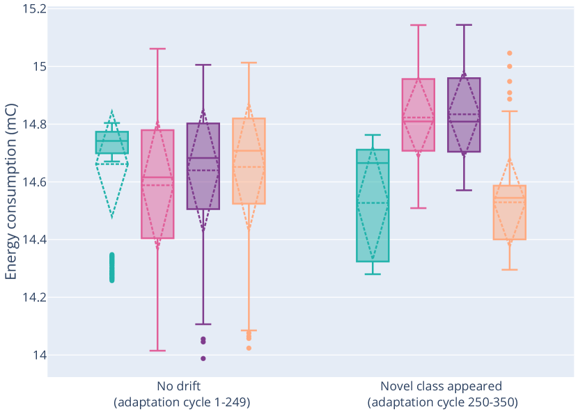
(b) Energy consumption

Figure 19. Quality properties of lifelong self-adaptation compared to the other approaches for the base scenario.

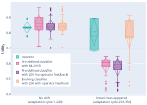
Figure 20. Impact of drift of adaptation spaces on the utility of the system.

In terms of RSM we observe similar results, see Figure 21. Without drift the three approaches perform close to the baseline (RSM of 0.002 for the pre-defined classifier with ML2ASR, 0.002 for the pre-defined classifier with LSA (no operator feedback), and 0.000 for the pre-defined classifier with LSA with operator feedback. On the other hand, with a drift of adaptation spaces, the RSM for the pre-defined classifier with ML2ASR, and the pre-defined classifier with LSA (no operator feedback) increase dramatically (to 0.55 and 0.54 respectively). On the contrary, the predictions of the pre-defined classifier with LSA with operator remain accurate with an RSM of 0.06.

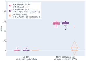
Figure 21. Impact of drift of adaptation spaces on the RSM for different approaches.

Conclusion.

In answer to EQ1, we can conclude that an evolving classifier with LSA with operator feedback is particularly effective in dealing with a drift of adaptation spaces, with a performance close to an ideal classifier with a perfect classification.

5.3.2. Robustness of Lifelong Self-Adaptation in Dealing with Drift of Adaptation Spaces.

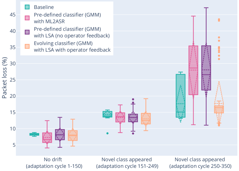
(a) $\langle$(B), R, G$\rangle$

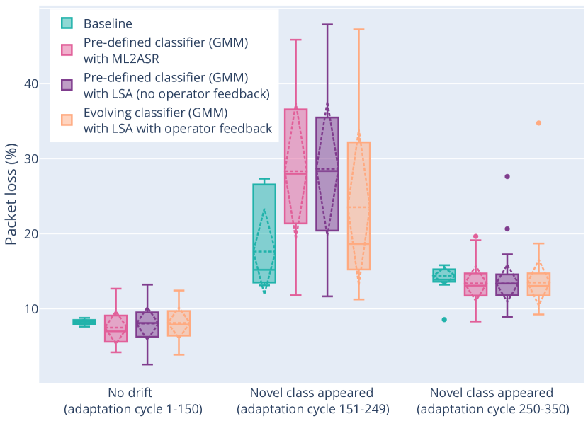
(b) $\langle$(B), G, R$\rangle$

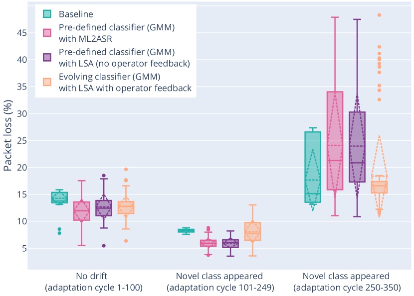
(c) $\langle$(R), B, G$\rangle$

(d) $\langle$(R), G, B$\rangle$

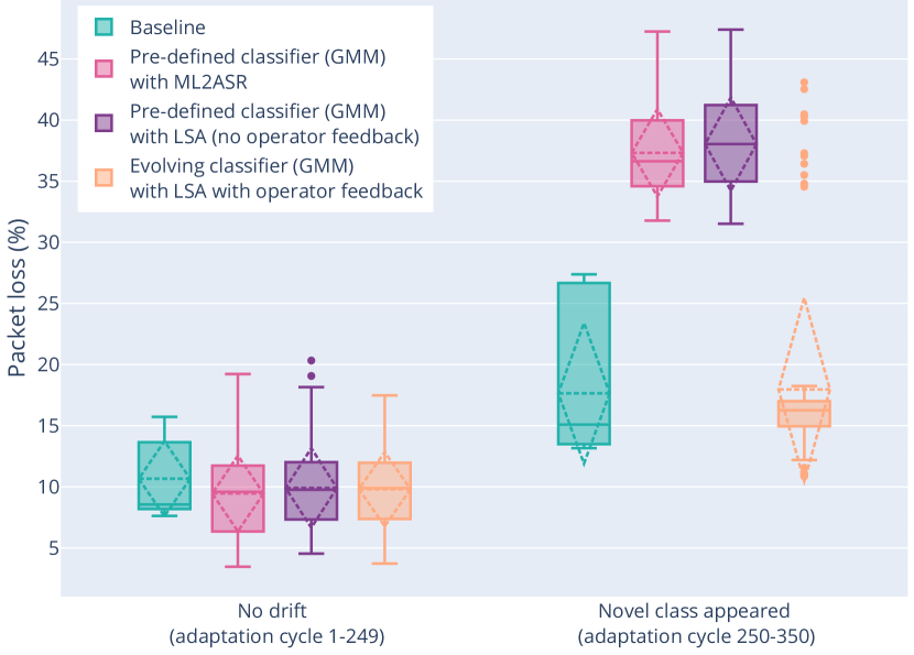
(e) $\langle$(B, R), G$\rangle$

(f) $\langle$(B, G), R$\rangle$

Figure 27. In terms of packet loss, evaluation of the lifelong self-adaptation with and without the feedback of the stakeholder by comparing with the state-of-the-art (the pre-defined classifier supported by ML2ASR), and the baseline. The preference of the stakeholder is here $\langle$“less packet loss”, “less energy consumption”$\rangle$. The appearance order of classes corresponding to each plot is mentioned in its caption.

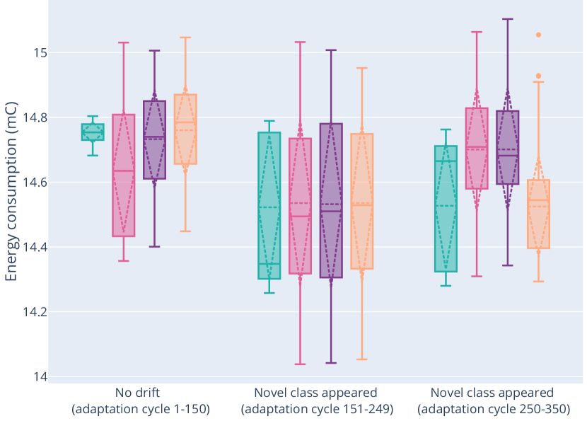
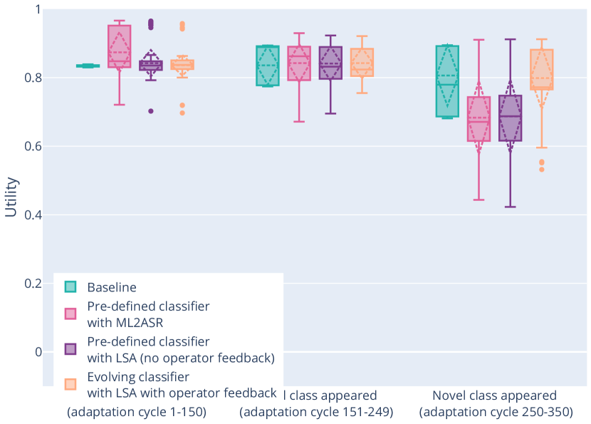
(a) $\langle$(B), R, G$\rangle$

(b) $\langle$(B), G, R$\rangle$

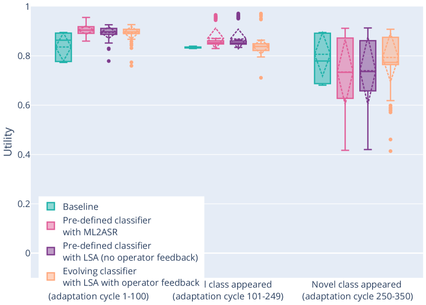
(c) $\langle$(R), B, G$\rangle$

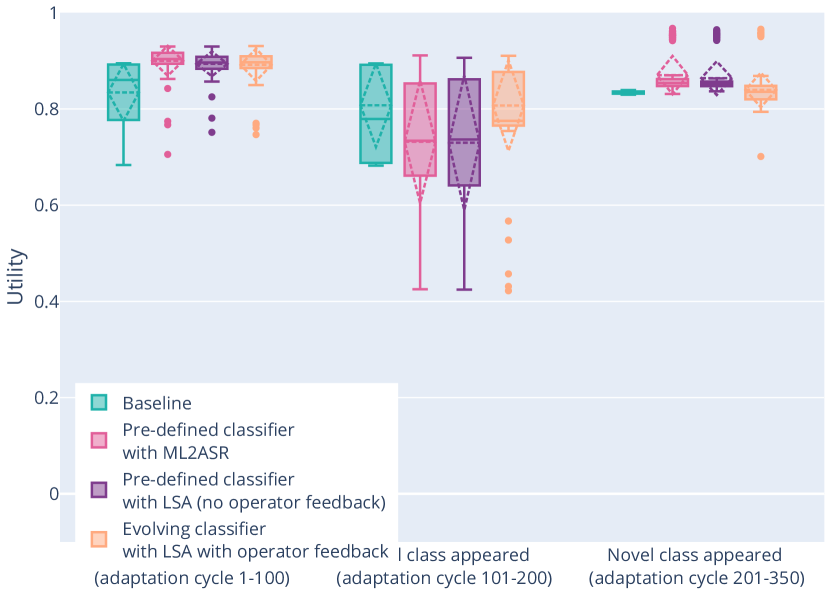
(d) $\langle$(R), G, B$\rangle$

(e) $\langle$(B, R), G$\rangle$

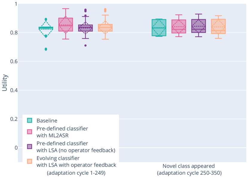
(f) $\langle$(B, G), R$\rangle$

Figure 28. In terms of energy consumption, evaluation of the lifelong self-adaptation with and without the feedback of the stakeholder by comparing with the state-of-the-art (the pre-defined classifier supported by ML2ASR), and the baseline. The preference of the stakeholder is here $\langle$“less packet loss”, “less energy consumption”$\rangle$. The appearance order of classes corresponding to each plot is mentioned in its caption.

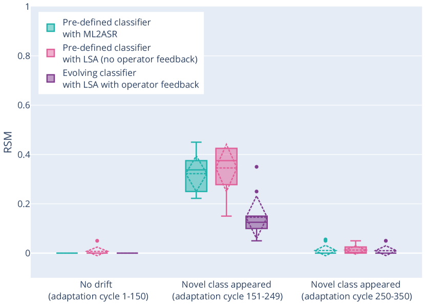
(b) $\langle$(B), G, R$\rangle$

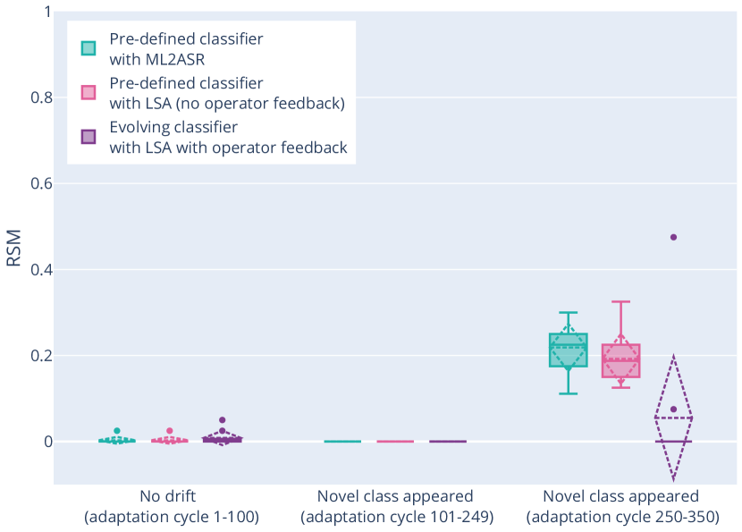
(c) $\langle$(R), B, G$\rangle$

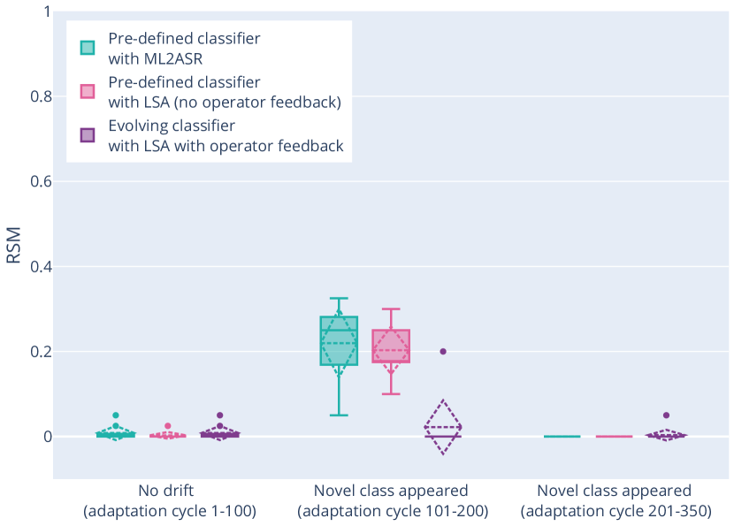
(d) $\langle$(R), G, B$\rangle$

(e) $\langle$(B, R), G$\rangle$

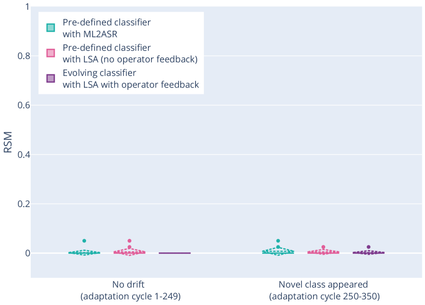
(f) $\langle$(B, G), R$\rangle$

Figure 29. In terms of utility, evaluation of the lifelong self-adaptation with and without the feedback of the stakeholder by comparing with the state-of-the-art (the pre-defined classifier supported by ML2ASR), and the baseline. The preference of the stakeholder is here $\langle$“less packet loss”, “less energy consumption”$\rangle$ (by weight of 0.8 and 0.2). The appearance order of classes corresponding to each plot is mentioned in its caption.

(a) $\langle$(B), R, G$\rangle$

(b) $\langle$(B), G, R$\rangle$

(c) $\langle$(R), B, G$\rangle$

(d) $\langle$(R), G, B$\rangle$

(e) $\langle$(B, R), G$\rangle$

(f) $\langle$(B, G), R$\rangle$

Figure 30. The impact of drift on the RSM value. In each group, bars indicate the value of RSM for: (i) the predefined classifier, (ii) the state-of-the-art (the pre-defined classifier supported by ML2ASR), (iii) lifelong self-adaptation without and (iv) with the feedback of the stakeholder, respectively from left to right. Also, the related class appearance order is determined in the caption of each figure. The preference of the stakeholder is here $\langle$“less packet loss”, “less energy consumption”$\rangle$.

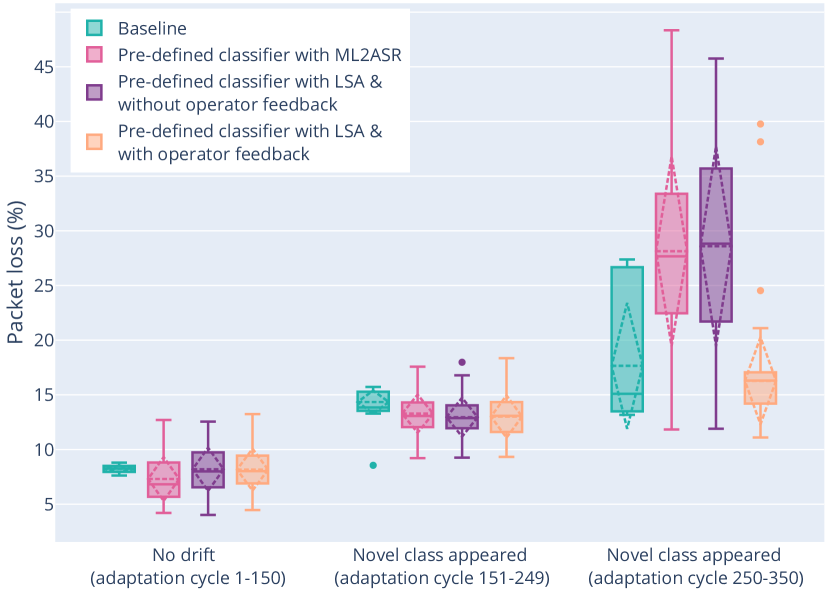
(a) $\langle$(B), R, G$\rangle$

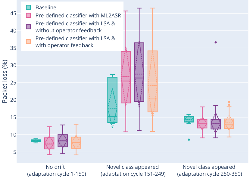
(b) $\langle$(B), G, R$\rangle$

(c) $\langle$(R), B, G$\rangle$

(d) $\langle$(R), G, B$\rangle$

(e) $\langle$(B, R), G$\rangle$

(f) $\langle$(B, G), R$\rangle$

Figure 31. In terms of packet loss, evaluation of the lifelong self-adaptation with and without the feedback of the stakeholder by comparing with the state-of-the-art (the pre-defined classifier supported by ML2ASR), the pre-defined classifier, and the baseline. The preference of the stakeholder is here $\langle$“less energy consumption”, “less packet loss”$\rangle$. The appearance order of classes corresponding to each plot is mentioned in its caption.

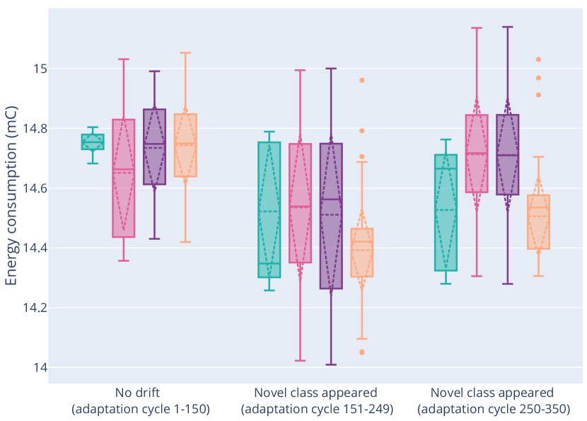
(a) $\langle$(B), R, G$\rangle$

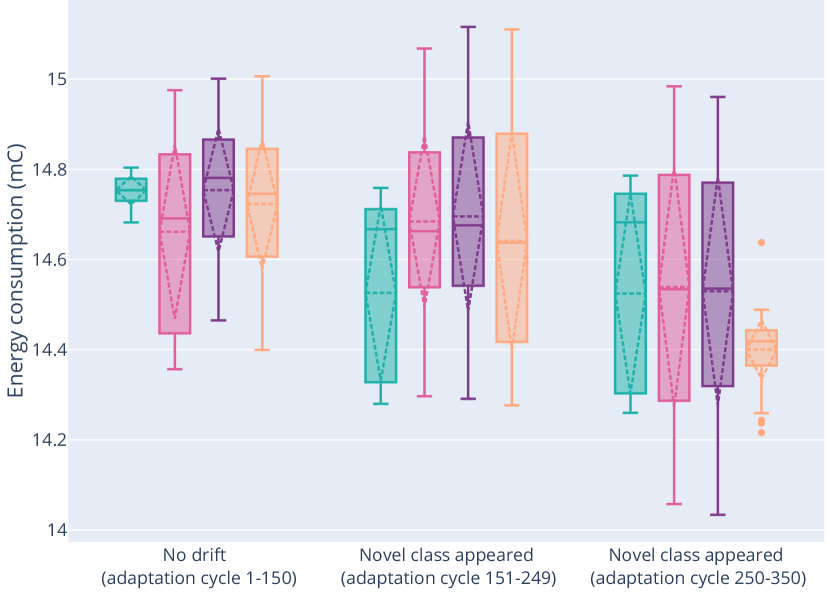
(b) $\langle$(B), G, R$\rangle$

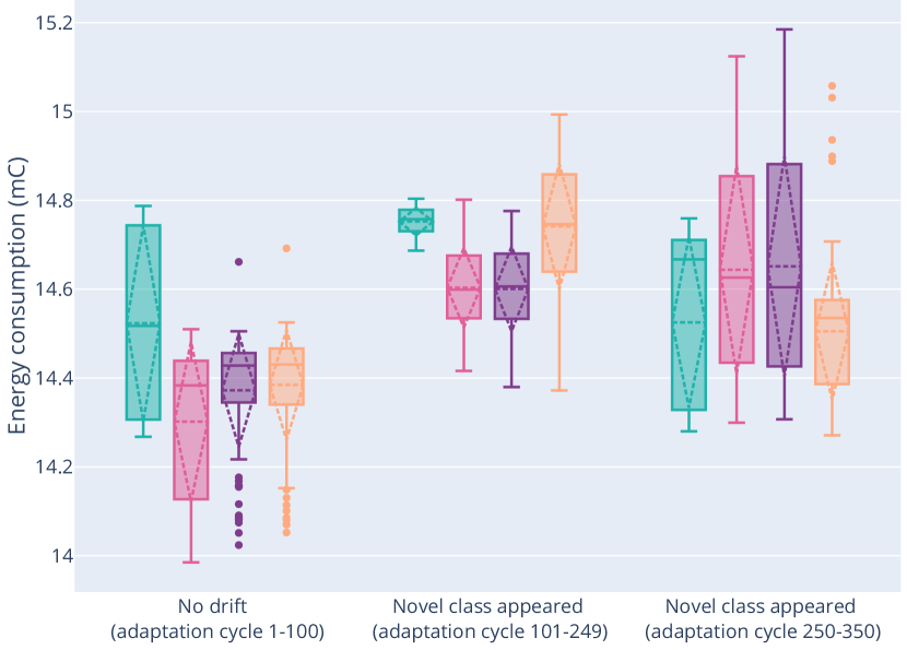
(c) $\langle$(R), B, G$\rangle$

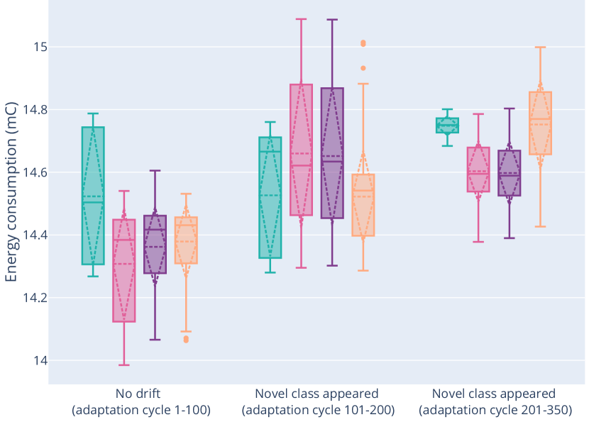
(d) $\langle$(R), G, B$\rangle$

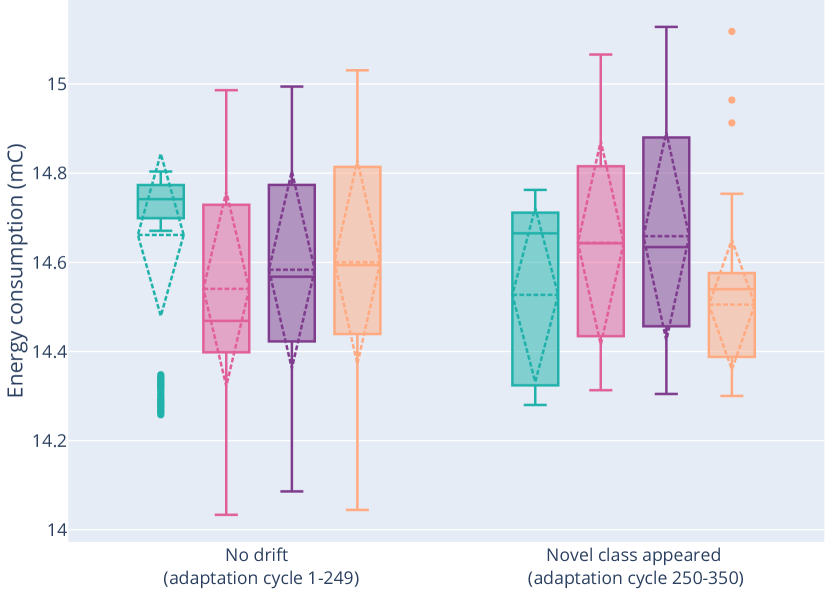
(e) $\langle$(B, R), G$\rangle$

(f) $\langle$(B, G), R$\rangle$

Figure 32. In terms of energy consumption, evaluation of the lifelong self-adaptation with and without the feedback of the stakeholder by comparing with the state-of-the-art (the pre-defined classifier supported by ML2ASR), the pre-defined classifier, and the baseline. The preference of the stakeholder is here $\langle$“less energy consumption”, “less packet loss”$\rangle$. The appearance order of classes corresponding to each plot is mentioned in its caption.

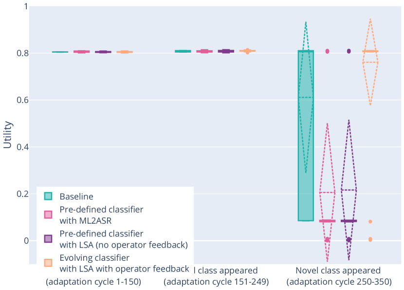
(a) $\langle$(B), R, G$\rangle$

(b) $\langle$(B), G, R$\rangle$

(c) $\langle$(R), B, G$\rangle$

(d) $\langle$(R), G, B$\rangle$

(e) $\langle$(B, R), G$\rangle$

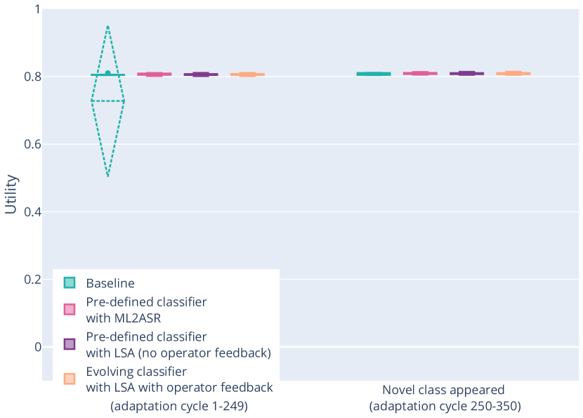
(f) $\langle$(B, G), R$\rangle$

Figure 33. In terms of utility, evaluation of the lifelong self-adaptation with and without the feedback of the stakeholder by comparing with the state-of-the-art (the pre-defined classifier supported by ML2ASR), and the baseline. The preference of the stakeholder is here $\langle$“less energy consumption”, “less packet loss”$\rangle$ (by weight of 0.8 and 0.2). The appearance order of classes corresponding to each plot is mentioned in its caption.

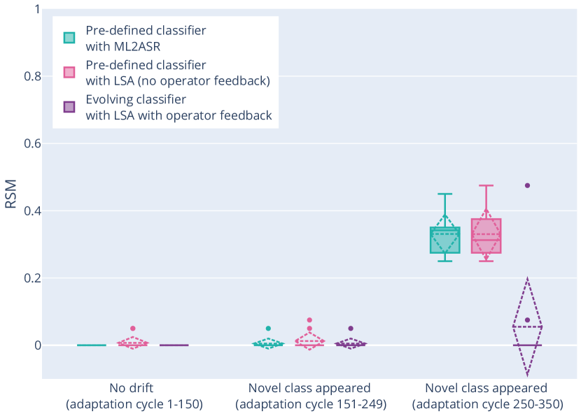
(a) $\langle$(B), R, G$\rangle$

(b) $\langle$(B), G, R$\rangle$

(c) $\langle$(R), B, G$\rangle$

(d) $\langle$(R), G, B$\rangle$

(e) $\langle$(B, R), G$\rangle$

(f) $\langle$(B, G), R$\rangle$

Figure 34. The impact of drift on the RSM value. In each group, bars indicate the value of RSM for: (i) the predefined classifier, (ii) the state-of-the-art (the pre-defined classifier supported by ML2ASR), (iii) lifelong self-adaptation without and (iv) with the feedback of the stakeholder, respectively from left to right. Also, the related class appearance order is determined in the caption of each figure. The preference of the stakeholder is here $\langle$“less energy consumption”, “less packet loss”$\rangle$.

To answer EQ2, we evaluated the 24 scenarios based on Table 1. We measured the quality attributes, the utilities, and the RSM values for all scenarios. The detailed results are available in Appendix A (including all validation scenarios, see Figures 27, 28, 29, 30, 31, 32, 33, 34).

Here we summarize the results for the utilities and RSM over all scenarios (during the period that new classes emerge). We start by looking at the robustness with respect to the appearance order of classes. Then we look at robustness with respect to the preference order of stakeholders.

Robustness with respect to the appearance order of classes.

Figure 22 shows the results of the utilities for the six scenarios of the appearance order of classes. The results indicate that the evolving classifier with LSA and operator feedback outperforms the pre-defined classifier with ML2ASR and the pre-defined classifier with LSA (no operator feedback) for scenarios (a), (b), and (e). For scenario (a) the mean utility is 0.80 for the evolving classifier with LSA and operator feedback versus 0.63 and 0.64 for the pre-defined classifier with ML2ASR and the pre-defined classifier with LSA (no operator feedback) respectively; for scenario (b) the mean utility was 0.70 versus 0.65 for both other approaches, and for scenario (e) the results are 0.78 versus 0.50 and 0.49 respectively. With a significance level of 0.05, the results of Mann-Withney U tests support the hypotheses that the utility of the evolving classifier with LSA and operator feedback is higher than the utility of the pre-defined classifier with ML2ASR and the utility of the pre-defined classifier with LSA in these scenarios (p = 0.000 for the three scenarios). For the other scenarios, the test results do not support the hypotheses. These scenarios do not seem to present a real challenge as all classifiers were able to achieve high mean utilities. On the other hand, the evolving classifier with LSA and operator feedback performs similarly to the baseline for all scenarios (difference in mean utilities between 0.004 and 0.068). With a significance level of 0.05, the results of Mann-Whitney U tests do not support the hypothesis that the utility of the baseline would be higher than the utility of the evolving classifier with LSA and operator feedback (p-values between 0.638 and 0.997 for the six scenarios).

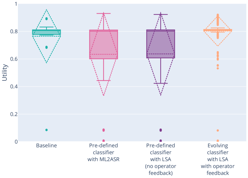
(a) $\langle$(B),R, G$\rangle$

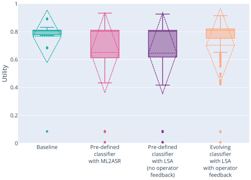
(b) $\langle$(B),G,R$\rangle$

(c) $\langle$(R),B,G$\rangle$

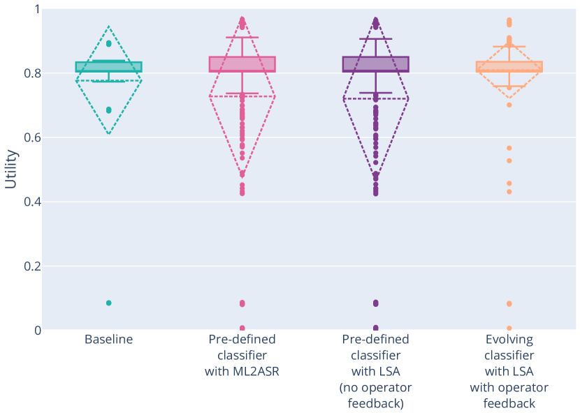
(d) $\langle$(R),G, B$\rangle$

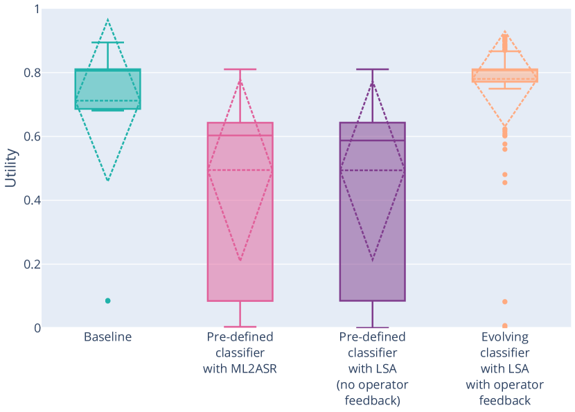
(e) $\langle$(B, R),G$\rangle$

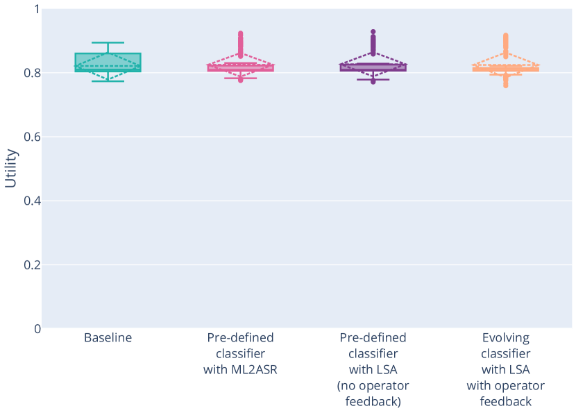
(f) $\langle$(B,G),R$\rangle$

Figure 22. Utility for all preference orders of stakeholders split for classes appearance orders.

The results for RSM shown in Figure 23 confirm the superiority of the evolving classifier with LSA and operator feedback compared to the other approaches. For scenarios (a) to (e), the difference between the mean RSM of the evolving classifier with LSA and operator feedback and the pre-defined classifier with ML2ASR is between 0.069 and 0.401, while the difference with the pre-defined classifier with LSA (no operator feedback) is between 0.065 and 0.342. With a significance level of 0.05, the results of Mann-Whitney U tests support the hypotheses that the RSM of the evolving classifier with LSA and operator feedback is lower than the other approaches (p-values between 0.000 and 0.028). For scenario (f), the difference between the mean RSM of the evolving classifier with LSA and operator feedback and the pre-defined classifier with ML2ASR is 0.005 and the difference with the pre-defined classifier with LSA (no operator feedback) is 0.001. With a significance level of 0.05, for this scenario, the results of Mann-Whitney U tests do not support the hypotheses that the RSM of the evolving classifier with LSA and operator feedback is lower than the two other approaches (p-values 0.341 and 0.447 respectively). The absolute results of the mean values for RSM for the evolving classifier with LSA and operator feedback (between 0.031 and 0.145 for the six scenarios) indicate a very good performance of the approach, comparable with an ideal classifier.

(a) $\langle$(B),R, G$\rangle$

(b) $\langle$(B),G,R$\rangle$

(c) $\langle$(R),B,G$\rangle$

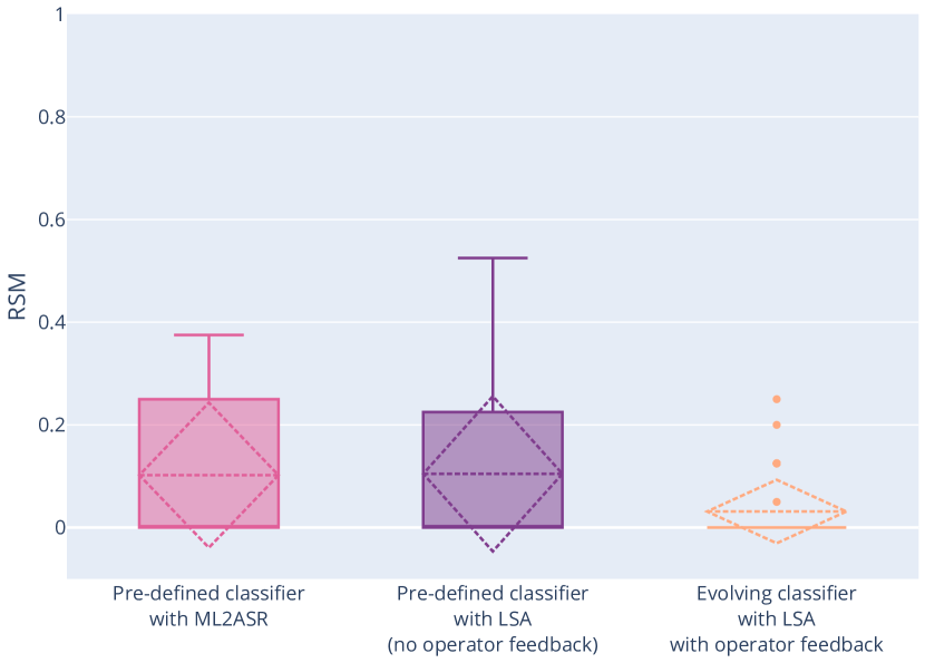
(d) $\langle$(R),G, B$\rangle$

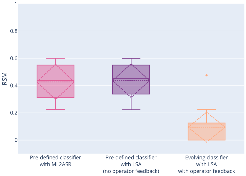
(e) $\langle$(B, R),G$\rangle$

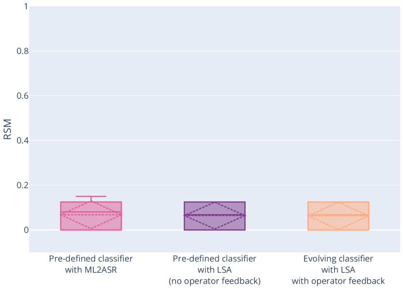
(f) $\langle$(B,G),R$\rangle$

Figure 23. RSM values for all preference orders of stakeholders split for classes appearance order.

Robustness with respect to the preference order of stakeholders.

For the preference order of stakeholders, we look at two scenarios (a) $\langle$”less packet loss,” ”less energy consumption”$\rangle$, and (b) $\langle$”less energy consumption,” ”less packet loss”$\rangle$. Figure 24(b) shows the utilities for scenario (b). The pre-defined classifier with ML2ASR and the pre-defined classifier with LSA (no operator feedback) perform similarly with the same mean utility of 0.59. The evolving classifier with LSA and operator feedback with a mean utility of 0.76 outperforms the pre-defined classifier with ML2ASR and the pre-defined classifier with LSA (no operator feedback), i.e., a difference in mean utility of 0.16 and 0.17 respectively. When we compare the mean utility of the evolving classifier with LSA and operator feedback with the baseline we observe a small difference in utility of 0.04. Figure 24(a)) shows the utilities for scenario (a). Here too, the pre-defined classifier with ML2ASR and the pre-defined classifier with LSA (no operator feedback) perform similarly with the same mean utility of 0.78. Yet, the difference in the mean utility for the evolving classifier with LSA and operator feedback with the other approaches is smaller, namely 0.03 and 0.04 compared to the pre-defined classifier with ML2ASR and the pre-defined classifier with LSA (no operator feedback). For the mean utility of the evolving classifier with LSA and operator feedback with the baseline, we observe again a small difference in utility of 0.05. With a significance level of 0.05, the test results of Mann-Withney U tests for both scenarios and additionally Wilcoxon signed-rank tests for scenario (a) support the following hypotheses in both scenarios: (i) the utility of evolving classifier with LSA and operator feedback is higher than the utility of the pre-defined classifier with ML2ASR and (ii) the utility of evolving classifier with LSA and operator feedback is higher than the utility of the pre-defined classifier with LSA. Furthermore, for both scenarios, the test results do not provide support that the utility of the baseline is higher than the utility of the evolving classifier with LSA and operator feedback. From a practical point of view, the difference in the mean utility of the evolving classifier with LSA and operator feedback with the baseline is negligible; so we can conclude that the evolving classifier with LSA and operator feedback performs close to the ideal classifier.

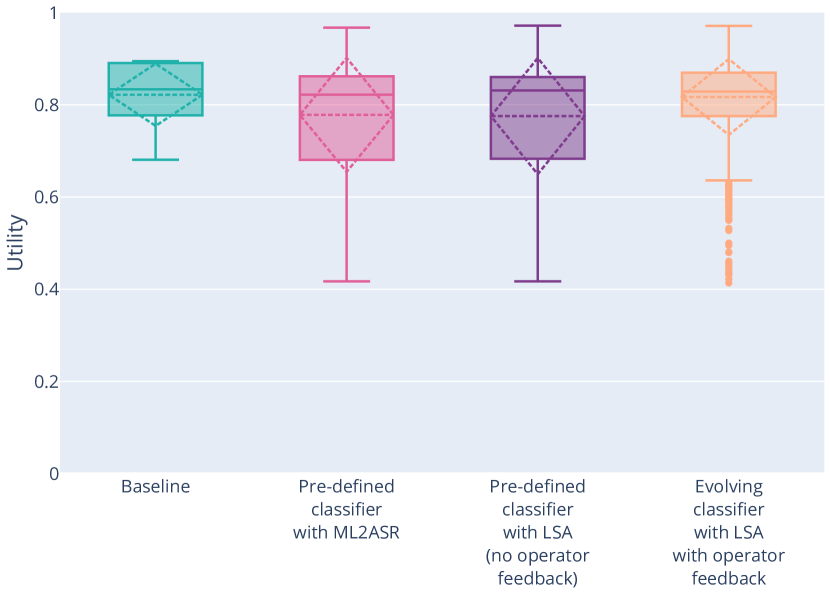
(a) $\langle$“less packet loss”, “less energy consumption”$\rangle$

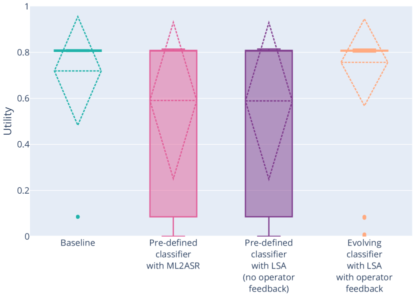
(b) $\langle$“less energy consumption”, “less packet loss”$\rangle$

Figure 24. Utility for all class appearance order scenarios split for preference order of stakeholders.

The results for the mean RSM confirm these analyses. Figure 25(b) shows the results for scenario (b). The pre-defined classifier with ML2ASR and the pre-defined classifier with LSA (no operator feedback) perform similarly, with the same mean RSM of 0.20. The mean RSM is 0.09 lower for the evolving classifier with LSA and operator feedback compared to both other approaches (0.11 versus 0.20 respectively). Figure 25(a) shows the results for scenario (a). Here too, the pre-defined classifier with ML2ASR and the pre-defined classifier with LSA (no operator feedback) perform similarly, with the same mean RSM of 0.15. The mean RSM of the evolving classifier with LSA and operator feedback is 0.12 lower compared to the pre-defined classifier with ML2ASR and the pre-defined classifier with LSA (no operator feedback) (0.03 versus 0.15 respectively). With a significance level of 0.05, the results of Mann-Withney U tests for both scenarios support the hypotheses: (i) the RSM of evolving classifier with LSA and operator feedback is less than the RSM of the pre-defined classifier with ML2ASR, and (ii) the RSM of evolving classifier with LSA and operator feedback is less than the RSM of the pre-defined classifier with LSA. The RSM for the evolving classifier with LSA and operator feedback are in both scenarios close to zero (0.11 and 0.03 for scenarios (b) and (a) respectively) indicating that the performance of the classifier is close to the ideal classifier.

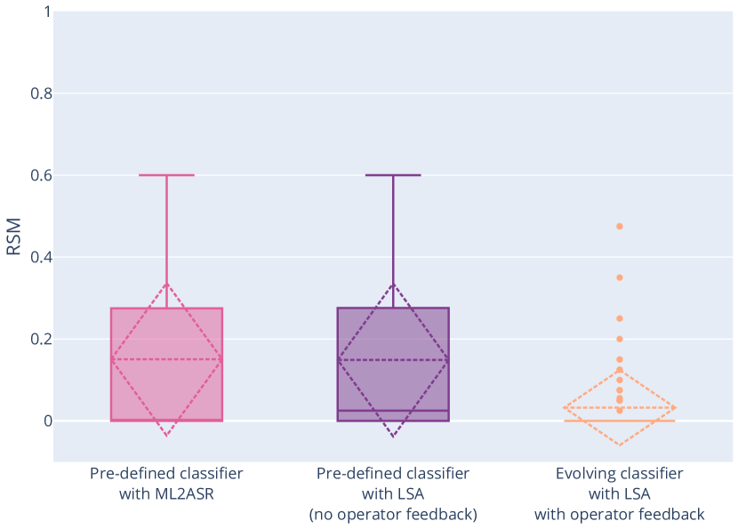
(a) $\langle$“less packet loss”, “less energy consumption”$\rangle$

(b) $\langle$“less energy consumption”, “less packet loss”$\rangle$

Figure 25. RSM values for all class appearance order scenarios split for preference order of stakeholders.

Conclusion.

In answer to EQ2, we can conclude that an evolving classifier with LSA with operator feedback is robust both to different appearance order of classes and to different preference orders of the stakeholder, and this is for all evaluated scenarios (while the results indicate that the competing approaches are not robust in half of the scenarios; the other half seem non-challenging scenarios).

5.3.3. Effectiveness of Operator Feedback in Lifelong Self-Adaptation for Dealing with Drift of Adaptation Spaces.

To answer EQ3, we leverage the results presented above for the 24 scenarios.

Figure 26(a) summarises the effect on the utility of the system over all scenarios for the pre-defined classifier with LSA with and without operator feedback. The difference of 0.11 in the mean utility (mean 0.79 with operator feedback and 0.68 without) shows that operator feedback contributes substantially to the utility of a self-adaptive system that faces drift of adaptation options. With a significance level of 0.05, the result of a Mann-Whitney U test supports the hypothesis that the utility of the evolving classifier with LSA and operator feedback is higher than the utility of the evolving classifier with LSA without operator feedback (p-value 0.000).

Figure 26(b) summarises the effect of operator involvement on the RSM. The results for RSM confirm the important role of the operator in dealing with a drift of adaptation spaces in self-adaptive systems. The difference in the mean of RSM is 0.11 lower with operator feedback (mean 0.07 without operator feedback and 0.18 with feedback). With a significance level of 0.05, the result of a Mann-Withney U test supports the hypothesis that the RSM of the evolving classifier with LSA and operator feedback is less than the RSM of the evolving classifier with LSA without operator feedback (p-value 0.000).

The boxplots also show that the interquartile ranges (i.e., the range between the 25 and the 75 percentile) for both metrics are substantially smaller for the classifier with operator feedback ([0.80, 0.82], i.e., 0.02 versus [0.64, 0.83], i.e., 0.19 for utility and [0.00, 0.13] versus [0.00, 0.33] for RSM). This shows that the classifier with operator feedback provides high-quality decisions in most of the adaptation cycles, which is not the case for the classifier without operator feedback.

(a) Impact on utilities.

(b) Impact on RSM.

Figure 26. Impact of the operator feedback on utilities and RSM in all scenarios.

Conclusion.

In answer to EQ3, we can conclude that operator feedback is particularly effective in dealing with drift of adaptation spaces; in fact operator feedback is essential.

5.4. Threats to Validity

The evaluation of lifelong self-adaptation to deal with drift of adaptation spaces is subject to a number of validity threats. To that end, we follow the guidelines provided in (Wohlin et al., 2012; Wieringa, 2014).

5.4.1. Construct Validity

Construct validity is about whether we have obtained the right measures to evaluate the proposed approach. Since there is (to the best of our knowledge) no competing approach that deals with shift of adaptation spaces in learning-based self-adaptive systems, we compared the proposed approach with a baseline (with an ideal classifier) and a state-of-the-art approach that uses learning in the analysis stage of self-adaptation. We used the impact on the quality properties as a primary metric to measure the usefulness of the approach in comparison with the other approaches. To measure the satisfaction level of the stakeholders of the system, we then computed the utility (using the data of the quality attributes) and the ranking satisfaction mean based on the classification of the selected adaptation options to compare the different approaches.

5.4.2. Internal Validity

Internal validity concerns drawing a causal conclusion based on the study. We have evaluated the instances of the architecture for the DeltaIoT case using particular settings. The type and number of new emerging classes generated in these settings may have an effect on the difficulty of the problems. We mitigated this threat by instantiating the architecture for in total of 24 different scenarios. These scenarios consider different patterns in new emerging classes. However, additional evaluation for other instances and in other domains is required to increase the validity of the results for the type of concept drift we studied.

5.4.3. External Validity

External validity concerns the generalization of the study results. We evaluated the approach only for one type of learner used in self-adaptive systems, so we cannot generalize the findings for other types of learners that require dealing with a new shift in adaptation spaces. Additional research is required to study the usefulness of the approach and the architecture for other use cases of learning that may be affected by a drift of adaptation spaces. Additionally, we validated the architecture with a single application. Evaluation in different domains is required to increase the validity of the results for the type of concept drift considered in this paper.

5.4.4. Reliability

For practical reasons, we used the simulator of the DeltaIoT network. For the evaluation we used data that contains uncertainty. Hence, the results may not necessarily be the same if the study would be repeated. We minimized this threat by considering stochastic data that was based on observations from real settings of the network, and we evaluated the different scenarios over long periods of time. We also provide a replication package for the study (Gheibi and Weyns, 2024).

5.4.5. Statistical Conclusion

Statistical conclusion validity concerns the degree to which conclusions drawn from statistical data analyses are accurate and appropriate (Iftikhar et al., 2017). To ensure that we have used proper statistical tests, we checked the distribution of the data and applied appropriate statistical tests based on the characteristics of the data. On the other hand, we acknowledge that the p-values that demonstrate statistical relevance are based on a limited set of experiments. To enhance the statistical significance of these results, repeated experiments or studies are needed that can confirm the results obtained in this paper. We leave this as an option for future work.

6. Related Work

We look at a selection of work at the crossing of machine learning and self-adaptation, focusing on approaches for (i) dealing with concept drift in machine learning, (ii) dealing with concept drift in self-adaptive systems, (iii) improving the performance of machine learning in self-adaptive systems, and (iv) dealing with unknowns in self-adaptive systems.

6.1. Dealing with Concept Drift in Machine Learning

Lu et al. (Lu et al., 2018) studied concept drift in the machine learning literature and identified two main research areas: drift detection and drift adaptation. Based on the methods described in the literature they proposed a general architecture that comprises four stages of concept drift detection in data stream analysis. Stage 1 retrieves chunks of data from data streams and organizes them to form a meaningful pattern. Stage 2 (optional) abstracts the data and extracts key features. Stage 3 calculates dissimilarity between data sets and was considered as the most challenging aspect of concept drift detection. Stage 4 uses a specific hypothesis test to evaluate the statistical significance of the change observed in Stage 3 to accurately determine the detection of drift. Compared with our general architecture, Stage 1 is part of the process of data collection performed by the knowledge manager. Stage 2 to Stage 4 can be part of task identification in the task manager. Therefore, existing detection methods seem to fit appropriately into our proposed general architecture.

When drift is detected, it needs to be managed. The method required to manage drift depends on the type of detected drift. Three main groups of methods were proposed by Lu et al. (Lu et al., 2018): training a new model, ensemble training, and model adjusting. Training a new model uses the latest data to replace the obsolete model, which maps to a structural change. Ensemble methods reused old models for recurring drifts, while model adjusting develops a model that adaptively learns from changing data; hence, decision tree algorithms were commonly used for this approach. Both ensemble methods and model-adjusting approaches could be considered instances of parametric changes. These three adaptation methods could be applied at any point in the data stream.

The general architecture for lifelong self-adaptation includes all the necessary elements for drift adaptation. The task manager is responsible for drift detection and understanding, such as when, how, and where the drift occurs (e.g., using previously detected tasks to handle recurrent drift). The task-based knowledge miner is responsible for mining useful data for adapting the learning model. The knowledge-based learner is responsible for adapting the learning model based on the task-based knowledge-mined data. Meanwhile, the knowledge manager collects all required data for the operation of other components in the lifelong learning layer. Therefore, all proposed drift adaptation methods can be integrated into our proposed general architecture.

6.2. Dealing with Concept Drift in Self-Adaptation

T. Chen (Chen, 2019) studied the impact of concept drift on machine learning models caused by uncertainties; focusing on models used by a self-adaptive system to evaluate and predict performance to make proper adaptation decisions. Two methods were studied: retrained modeling that always discarded the old model and retrained a new one using all available data, and incremental modeling that retained the existing model and tuned it using one newly arrived data sample. Usually, the choice for one of them was based on general beliefs. In contrast, the author reported an empirical study that examined both modeling methods for distinct domains of adaptable software and identified evidence-based factors that could be used to make well-informed decisions for choosing a method.

Bierzynski et al. (Bierzynski et al., 2019) presented the architecture of a self-learning lighting system that equips a MAPE-K loop with a learner that learns activities and user preferences. The learner is equipped with a dedicated component that realizes another feedback loop on top of the learner. This inner feedback loop determines when the predictions of a model start to drift and then adapts the learning model accordingly. Previously recognized drift patterns are exploited to enhance the performance of new drift and minimize the need for human intervention. The authors proposed a concrete implementation based on the micro-service pattern and evaluated the result with different other architectural patterns, e.g., Mikrokernel and Monolith.

Vieira et al. (Vieira et al., 2021) proposed Driftage, a multi-agent systems framework to simplify implementing concept drift detectors. The framework divides concept drift detection responsibilities between agents. The approach is realized as a MAPE-K loop, where monitor and analyzer agents capture and predict concept drifts in data, and planner and executor agents determine whether the detected concept drift should be alerted. The authors illustrated their approach in the domain of health monitoring of muscle cells, combining different types of learners who vote for detecting drift.

Casimiro et al. (Casimiro et al., 2021) discussed the implications of unexpected changes, e.g., drifts in the input data on using machine learning-based systems. The authors proposed a framework for self-adaptive systems that relies on machine-learned components. The paper outlined (i) a set of causes of misbehavior of machine-learned components and a set of adaptation tactics inspired by the literature, (ii) the required changes to the MAPE-K loop for dealing with the unexpected changes, and (iii) the challenges associated with developing this framework.

In contrast to these approaches, we provide a general domain-independent architecture to deal with all types of concept drift in learning modules with variant learning tasks (i.e., regression and classification) used by self-adaptive systems. The work of (Chen, 2019) and (Casimiro et al., 2021) offer valuable solutions that can be used when instantiating the architecture for lifelong self-adaptation.

6.3. Improving the Performance of Machine Learning for Self-Adaptation

Jamshidi et al. (Jamshidi et al., 2018) proposed an efficient approach for transferring knowledge across highly configurable environments to simplify the configuration, e.g., hardware, workload, and software release. The approach, called L2S (Learning to Sample), selects better samples in the target environment based on information from the source environment. L2S progressively shrinks and adaptively concentrates on interesting regions of the configuration space. The authors demonstrated that L2S outperformed state-of-the-art learning and transfer-learning approaches in terms of measurement effort and learning accuracy.

T. Chen and Bahsoon (Chen and Bahsoon, 2017) presented a self-adaptive modeling approach that leverages information theory and machine learning algorithms to create a quality model for predicting a quality property over time by using data on environmental conditions and the control settings as inputs. Concretely, the authors used self-adaptive hybrid dual-learners that partition the input space in two sub-spaces, each applying a different symmetric uncertainty-based selection technique; the results of sub-spaces were then combined. The authors then used adaptive multi-learners for building the model of the QoS function, supporting selecting the best model for prediction on the fly. The approach was evaluated in a cloud environment. X. Chen et al. (Chen et al., 2019) applied a similar approach to deal with the problem of resource allocation for cloud-based software services.

T. Chen et al. (Chen et al., 2010) proposed the notion of “experience transfer” to utilize knowledge learned from one system to another similar system. The transfer process discovers and represents transferable experiences, extracts the experiences during the modeling process in the original system, and embeds learned experiences into the management of the new system. The authors demonstrated the process and benefits of experience transfer for system configuration tuning using a Bayesian network. In this case, the dependencies between configuration parameters are valuable experiences.

These related approaches targeted the efficiency of machine learning methods in the context of self-adaptation. Our work complements these approaches focusing on enhancing learning to handle new learning tasks as required for concept drift and drift of adaptation spaces in particular.

6.4. Dealing with Unknowns in Self-Adaptive Systems

Kinneer et al. (Kinneer et al., 2018) focused on the change of the adaptive logic in response to changes, such as the addition or removal of adaptation tactics. The authors argue that such changes in a self-adaptive system often require a human planner to redo expensive planning. To address this problem the authors proposed a planner based on genetic programming that reuses existing plans. The authors demonstrated that naïvely reusing existing plans for planning in self-adaptive systems results in a loss of utility. This work fits in a line of research on automatic (re-)generation of adaptive logic to deal with circumstances that are hard to anticipate before the deployment of the system.

Palm et al. (Palm et al., 2020) integrated a policy-based reinforcement learner with the MAPE-K architecture to deal with environment changes that are difficult or impossible to anticipate before deployment of the system. Different from traditional online reinforcement learning approaches for self-adaptive systems that require manual fine-tuning of the exploration rate and quantizing environment states, the proposed approach automates these manual activities. To demonstrate the feasibility and applicability, the authors validated the proposed approach in two domains, namely to balance workloads in a web application subject to multiple types of drifts in the distribution of the workload, and to predict the behavior of a process in a business process management system when there is a shift in process behavior. The experiments show that there is room for improvement in the convergence of the reinforcement learning method and the ability to handle large adaptation spaces.

Krupitzer et al. (Krupitzer et al., 2016) coin the term self-improvement within self-adaptive systems as an adaptation of the adaptation logic that helps shift the integration tasks from the static design time to the runtime. The authors survey approaches for self-improvement, compare these approaches, and categorize them. The categorization highlights that the approaches focus either on structural or parameter adaptation but seldom combine both. From this insight, the authors outline a set of challenges that need to be addressed by future approaches for self-improvement.

Recently, Alberts and Gerostathopoulos (Alberts and Gerostathopoulos, 2022) focused on context shifts in learning-based self-adaptive systems. The authors proposed a new metric, convergence inertia, to assess the robustness of reinforcement learning policies against context shifts. This metric is then used to assess the robustness of different policies within a family of multi-armed bandits against context shifts. The authors argue through an experiment with a self-adaptation web server that inertia and the accompanying interpretation of the unknown-unknowns problem is a viable way to inform the selection of online learning policies for self-adaptive systems.

These related approaches exploited learning approaches to solve problems with unknown or unforeseen conditions in self-adaptive systems. Lifelong self-adaptation contributes to this line of research with an approach that enables a learning-based self-adaptive system to deal with new learning tasks with a focus on a drift of adaptation spaces.

7. Conclusions and Future Work

This paper started from the research problem ”how to enable learning-based self-adaptive systems to deal with drift of adaptation spaces during operation, i.e., concept drift in the form of novel class appearance?” We illustrated the potentially severe effect of a shift of adaptation in terms of achieving the quality attributes of the adaptation goals, the utility of self-adaptation, and the ranking satisfaction mean, a novel metric to measure the satisfaction level of stakeholders in terms of class ranking of the selected adaptation option of a pre-defined classifier versus an ideal classifier.

To tackle the research problem we presented a general architecture for lifelong self-adaptation that supports learning-based self-adaptive systems to deal with new learning tasks during operation. We instantiated the general architecture to deal with a drift of adaptation spaces using the DeltaIoT exemplar. Empirical results of 24 different scenarios demonstrate that lifelong self-adaptation is effective and robust to drift in adaptation spaces. The operator takes a key role in ranking classes, including new classes, in the lifelong learning loop that underlies lifelong self-adaptation.

As future work, the proposed approach of lifelong self-adaptation could be applied to the problem of drift of adaptation spaces for different scenarios and different application domains, adding to the external validity of the proposed approach. The knowledge extracted from such studies may yield solutions that may be reusable across domains. Another interesting line of future work could be dealing with dynamically changing goals. Yet another option for future work would be to study the challenges associated with catastrophic forgetting when applying lifelong self-adaptation. Beyond that, it would be interesting to study other problems that a learning-based self-adaptive system may face leveraging the generic approach of lifelong self-adaptation. One example could be the automatic generation of adaptation strategies (e.g., to reconfigure) under new encountered conditions. An inspiring example based on automatic synthesis is presented in (Nahabedian et al., 2022). Another example is employing lifelong self-adaptation for realizing situation awareness in self-adaptive systems, inspired by (Lesch et al., 2022). The task-manager component can play a central role in this way. In the long term, an interesting topic for research could be to investigate how lifelong self-adaptation can be enhanced to build systems that can truly evolve themselves. Inspiration in that direction can be found in research on self-improvement (Krupitzer et al., 2016) and self-evolution (Weyns et al., 2022).

Appendix A Complete Validation Scenarios

(a) $\langle$(B), R, G$\rangle$

Appendix B Statistical Analysis of the Evaluation Results

We present the statistical analysis of the evaluation results presented in the main text of the paper. The text is structured based on the figures of the evaluation as they appear in the main text.

In the following, $\mu_{i,j,k}$ represents the value under test of an approach, with $i$ representing the related subfigure with possible values $\{a,b,c,d,e,f\}$ (his set can be reduced to a subset depending on the number of subfigures of the corresponding figure - e.g., $\{a,b\}$ - or $i$ can be omitted when there are no subfigures, we then write $\mu_{j,k}$), $j$ represents the metric value with possible values $\{r,u\}$, with $r$ representing RSM and $u$ representing the utility, and $k$ represents the actual approach with possible values “Baseline”, “ML2ASR”, “LSA”, and “LSA with operator feedback”.

B.1. Quality Properties of Lifelong Self-Adaptation (Figure 19)

Figure 19 shows the quality properties of lifelong self-adaptation compared to the other approaches for the base scenario. Since the different approaches optimize for utility we cannot define hypotheses for individual quality properties. Hence, we only present basic statistics in Table 2 and Table 3.

Table 2. Statistics corresponding to Figure 19(a): packet loss in the base scenario

No drift Novel class appeared Median Mean Standard deviation Median Mean Standard deviation Approaches Baseline 8.556 10.665 3.072 15.093 17.654 5.751 ML2ASR 9.593 9.457 3.094 36.630 37.320 3.570 LSA 9.765 9.910 3.250 38.033 38.035 3.808 LSA with operator 9.895 9.813 3.040 16.263 17.962 7.503

Table 3. Statistics corresponding to Figure 19(b): energy consumption in the base scenario

No drift Novel class appeared Median Mean Standard deviation Median Mean Standard deviation Approaches Baseline 14.742 14.661 0.182 14.665 14.527 0.195 ML2ASR 14.616 14.588 0.226 14.809 14.823 0.139 LSA 14.683 14.640 0.215 14.809 14.834 0.152 LSA with operator 14.708 14.651 0.224 14.545 14.529 0.155

B.2. Impact of Drift of Adaptation Spaces on The Utility (Figure 20)

Figure 20 shows the impact of the drift of adaptation spaces on the utility of the system. Table 4 shows the basic statistics.

Table 4. Statistics corresponding to Figure  20: utility in the base scenario

No drift Novel class appeared Median Mean Standard deviation Median Mean Standard deviation Approaches Baseline 0.834 0.835 0.036 0.779 0.806 0.088 ML2ASR 0.843 0.862 0.054 0.606 0.589 0.052 LSA 0.837 0.845 0.040 0.591 0.577 0.058 LSA with operator 0.838 0.844 0.037 0.776 0.798 0.099

For the baseline and LSA with operator feedback when the novel class appeared, denoted by $\mu_{u,\text{Baseline}}$, $\mu_{u,\text{LSA with operator}}$ respectively, we define the following alternative hypothesis:

• The utility of the “Baseline” is higher than the utility of the “evolving classifier with LSA and operator feedback” when a novel class appeared:

  $$H_{1}: \mu_{u,\text{Baseline}}>\mu_{u,\text{LSA with operator}}$$

  $$H_{0}: \mu_{u,\text{Baseline}}=\mu_{u,\text{LSA with operator}}$$

We start with determining the appropriate test we can use to test the null hypothesis. First, we test whether the data of the utilities for the baseline and LSA with operator are normally distributed using the Anderson–Darling test (D’Agostino, 2017). Based on the results of Table 5, with a significance level ($\alpha$) of $0.05$, all normality tests were rejected.

Table 5. Normality tests for distributions in Figure 20, by Anderson-Darling test method.

Approach p-value Baseline 0.000 LSA with operator 0.000

Next, we use the Spearman correlation method (Myers et al., 2010) to test the dependency between the pair of data. With a significance level of 0.05, the test results shown in Table 6 indicate that the dependency test for the pair is rejected.

Table 6. Dependency test for distributions in Figure 20, by Spearman correlation test method.

Approach p-value (Baseline, LSA with operator) 0.000

Since both the normality test and the dependency test are rejected, we apply the Mann-Whitney U test (MacFarland and Yates, 2016) to test the null hypothesis in Table 7 for Figure 20.

Table 7. Test results for the hypothesis for Figure 20.

Hypothesis p-value Test method $H_{0}:\mu_{u,\text{Baseline}}=\mu_{u,\text{LSA with operator}}$ 0.114 Mann-Whitney U

With a significance level of 0.05, the test result does not support the alternative hypothesis. Hence, there is no evidence that the utility of the “Baseline” is higher than the utility of the “evolving classifier with LSA and operator feedback”.

B.3. Impact of Drift of Adaptation Spaces on The RSM (Figure 21)

Figure 21 shows the impact of drift of adaptation spaces on the RSM for the different approaches. As LSA with operator feedback clearly outperforms two other approaches, i.e., ML2ASR and LSA, in the base scenario after the appearance of a novel class, we only present basic statistics in Table 8.

Table 8. Statistics corresponding to Figure 21: RSM in the base scenario

No drift Novel class appeared Median Mean Standard deviation Median Mean Standard deviation Approaches ML2ASR 0.000 0.002 0.010 0.550 0.548 0.036 LSA 0.000 0.002 0.010 0.550 0.543 0.046 LSA with operator 0.000 0.000 0.000 0.000 0.055 0.141

B.4. Utility for All Preference Orders of Stakeholders Split For Classes Appearance Orders (Figure 22)

Figure 22 shows the utility for all preference orders of stakeholders split for the appearance orders of classes. Table 9 shows the basic statistics. We define the following set of alternative hypotheses:

Table 9. Statistics corresponding to Figure 22: utility for all preference orders of stakeholders

(a) (b) Median Mean Standard deviation Median Mean Standard deviation Approaches Baseline 0.806 0.765 0.192 0.806 0.767 0.189 ML2ASR 0.801 0.634 0.301 0.803 0.651 0.289 LSA 0.802 0.637 0.298 0.803 0.646 0.290 LSA with operator 0.809 0.803 0.110 0.809 0.703 0.264

(c) (d) Median Mean Standard deviation Median Mean Standard deviation Approaches Baseline 0.806 0.775 0.171 0.806 0.777 0.168 ML2ASR 0.807 0.728 0.251 0.808 0.728 0.250 LSA 0.808 0.756 0.253 0.808 0.721 0.256 LSA with operator 0.807 0.806 0.089 0.808 0.809 0.088

(e) (f) Median Mean Standard deviation Median Mean Standard deviation Approaches Baseline 0.806 0.712 0.253 0.810 0.821 0.042 ML2ASR 0.603 0.495 0.285 0.809 0.825 0.037 LSA 0.587 0.494 0.280 0.809 0.827 0.038 LSA with operator 0.807 0.780 0.149 0.809 0.825 0.039

• For each scenario $i$, the utility of the “Baseline” is higher than the utility of the “evolving classifier with LSA and operator feedback” when a novel class appeared:

  $$H_{1}^{(i)}: \mu_{i,u,\text{Baseline}}>\mu_{i,u,\text{LSA with operator}}$$

  $$H_{0}^{(i)}: \mu_{i,u,\text{Baseline}}=\mu_{i,u,\text{LSA with operator}}$$

• For each scenario $i$, the utility of the “evolving classifier with LSA and operator feedback” is higher than the utility of the “pre-defined classifier with ML2ASR”:

  $$H_{1}^{(i)}: \mu_{i,u,\text{LSA with operator}}>\mu_{i,u,\text{ML2ASR}}$$

  $$H_{0}^{(i)}: \mu_{i,u,\text{LSA with operator}}=\mu_{i,u,\text{ML2ASR}}$$

• For each scenario $i$, the utility of the “evolving classifier with LSA and operator feedback” is higher than the utility of the “pre-defined classifier with LSA”:

  $$H_{1}^{(i)}: \mu_{i,u,\text{LSA with operator}}>\mu_{i,u,\text{LSA}}$$

  $$H_{0}^{(i)}: \mu_{i,u,\text{LSA with operator}}=\mu_{i,u,\text{LSA}}$$

Note that the above generic hypotheses represent six distinct concrete hypotheses with the value of $i$ chosen from the set of scenarios $\{a,b,c,d,e,f\}$.

We start with determining the appropriate test we can use to test null hypotheses. First, we test whether the data of the utilities for each approach are normally distributed using the Anderson–Darling test. Based on the results of Table 10, with a significance level ($\alpha$) of $0.05$, all normality tests were rejected.

Table 10. Normality tests for distributions in subfigures of Figure 22, by Anderson-Darling test method

Approach p-value (a) p-value (b) p-value (c) p-value (d) p-value (e) p-value (f) Baseline 0.000 0.000 0.000 0.000 0.000 0.000 ML2ASR 0.000 0.000 0.000 0.000 0.000 0.000 LSA 0.000 0.000 0.000 0.000 0.000 0.000 LSA with operator 0.000 0.000 0.000 0.000 0.000 0.000

Next, we use the Spearman correlation method to test the dependency between related pairs of data. With a significance level of 0.05, the test results shown in Table 11 indicate that the dependency tests for all pairs are rejected.

Table 11. Dependency tests for distributions in subfigures of Figure 22, by Spearman correlation test method

Approach p-value (a) p-value (b) p-value (c) p-value (d) p-value (e) p-value (f) (Baseline, LSA with operator) 0.000 0.000 0.000 0.000 0.000 0.000 (ML2ASR, LSA with operator) 0.000 0.000 0.000 0.000 0.000 0.000 (LSA, LSA with operator) 0.000 0.000 0.000 0.000 0.000 0.000

Since both the normality and dependency tests are rejected for all cases, we apply the Mann-Whitney U test to test all the null hypotheses of Table 12 for Figure 22.

Table 12. Test results for all hypotheses for Figure 22, related hypotheses to each subfigure are separated by a double horizontal line from the others.

Hypothesis p-value Test method $H_{0}^{(a)}:\mu_{a,u,\text{Baseline}}=\mu_{a,u,\text{LSA with operator}}$ 0.953 Mann-Whitney U $H_{0}^{(a)}:\mu_{a,u,\text{LSA with operator}}=\mu_{a,u,\text{ML2ASR}}$ 0.000 Mann-Whitney U $H_{0}^{(a)}:\mu_{a,u,\text{LSA with operator}}=\mu_{a,u,\text{LSA}}$ 0.000 Mann-Whitney U $H_{0}^{(b)}:\mu_{b,u,\text{Baseline}}=\mu_{b,u,\text{LSA with operator}}$ 0.110 Mann-Whitney U $H_{0}^{(b)}:\mu_{b,u,\text{LSA with operator}}=\mu_{b,u,\text{ML2ASR}}$ 0.000 Mann-Whitney U $H_{0}^{(b)}:\mu_{b,u,\text{LSA with operator}}=\mu_{b,u,\text{LSA}}$ 0.000 Mann-Whitney U $H_{0}^{(c)}:\mu_{c,u,\text{Baseline}}=\mu_{c,u,\text{LSA with operator}}$ 0.767 Mann-Whitney U $H_{0}^{(c)}:\mu_{c,u,\text{LSA with operator}}=\mu_{c,u,\text{ML2ASR}}$ 0.747 Mann-Whitney U $H_{0}^{(c)}:\mu_{c,u,\text{LSA with operator}}=\mu_{c,u,\text{LSA}}$ 0.837 Mann-Whitney U $H_{0}^{(d)}:\mu_{d,u,\text{Baseline}}=\mu_{d,u,\text{LSA with operator}}$ 0.708 Mann-Whitney U $H_{0}^{(d)}:\mu_{d,u,\text{LSA with operator}}=\mu_{d,u,\text{ML2ASR}}$ 0.539 Mann-Whitney U $H_{0}^{(d)}:\mu_{d,u,\text{LSA with operator}}=\mu_{d,u,\text{LSA}}$ 0.598 Mann-Whitney U $H_{0}^{(e)}:\mu_{e,u,\text{Baseline}}=\mu_{e,u,\text{LSA with operator}}$ 0.638 Mann-Whitney U $H_{0}^{(e)}:\mu_{e,u,\text{LSA with operator}}=\mu_{e,u,\text{ML2ASR}}$ 0.000 Mann-Whitney U $H_{0}^{(e)}:\mu_{e,u,\text{LSA with operator}}=\mu_{e,u,\text{LSA}}$ 0.000 Mann-Whitney U $H_{0}^{(f)}:\mu_{f,u,\text{Baseline}}=\mu_{f,u,\text{LSA with operator}}$ 0.997 Mann-Whitney U $H_{0}^{(f)}:\mu_{f,u,\text{LSA with operator}}=\mu_{f,u,\text{ML2ASR}}$ 0.652 Mann-Whitney U $H_{0}^{(f)}:\mu_{f,u,\text{LSA with operator}}=\mu_{f,u,\text{LSA}}$ 0.809 Mann-Whitney U

With a significance level of 0.05, some test results support the corresponding alternative hypotheses, while other results do not. Concretely, we found evidence that: (i) the utility of the “evolving classifier with LSA and operator feedback” is higher than the utility of “ML2ASR” and utility of the “pre-defined classifier with LSA” in scenarios (a), (b), and (e). All the remaining alternative hypotheses are not supported by the test results. Concretely, we found no evidence that: (i) the utility of the “Baseline” is higher than the utility of the “evolving classifier with LSA and operator feedback” in all scenarios from (a) to (f), (ii) the utility of the “evolving classifier with LSA and operator feedback” is higher than the utility of the “ML2ASR” in scenarios (c), (d), and (f), and (iii) the utility of the “evolving classifier with LSA and operator feedback” is higher than the utility of the “pre-defined classifier with LSA” in scenarios (c), (d), and (f), the same as the “ML2ASR”.

B.5. RSM for All Preference Orders of Stakeholders Split for Classes Appearance Order (Figure 23)

Figure 23 illustrates the RSM for all preference orders of stakeholders split for classes appearance orders. Table 13 shows the basic statistics. We define the following set of alternative hypotheses:

Table 13. Statistics corresponding to Figure 23: RSM for all preference orders of stakeholders

(a) (b) Median Mean Standard deviation Median Mean Standard deviation Approaches ML2ASR 0.200 0.227 0.175 0.186 0.221 0.169 LSA 0.200 0.228 0.176 0.163 0.230 0.180 LSA with operator 0.118 0.082 0.092 0.125 0.145 0.115

(c) (d) Median Mean Standard deviation Median Mean Standard deviation Approaches ML2ASR 0.000 0.107 0.139 0.000 0.102 0.141 LSA 0.000 0.102 0.138 0.000 0.105 0.151 LSA with operator 0.000 0.038 0.085 0.000 0.031 0.062

(e) (f) Median Mean Standard deviation Median Mean Standard deviation Approaches ML2ASR 0.438 0.495 0.426 0.081 0.068 0.062 LSA 0.450 0.436 0.124 0.068 0.064 0.060 LSA with operator 0.118 0.094 0.110 0.068 0.063 0.061

• For each scenario $i$, the RSM of the “evolving classifier with LSA and operator feedback” is less than the RSM of the “pre-defined classifier with ML2ASR”:

  $$H_{1}^{(i)}: \mu_{i,r,\text{LSA with operator}}<\mu_{i,r,\text{ML2ASR}}$$

  $$H_{0}^{(i)}: \mu_{i,r,\text{LSA with operator}}=\mu_{i,r,\text{ML2ASR}}$$

• For each scenario $i$, the RSM of the “evolving classifier with LSA and operator feedback” is less than the RSM of the “pre-defined classifier with LSA”:

  $$H_{1}^{(i)}: \mu_{i,r,\text{LSA with operator}}<\mu_{i,r,\text{LSA}}$$

  $$H_{0}^{(i)}: \mu_{i,r,\text{LSA with operator}}=\mu_{i,r,\text{LSA}}$$

Here too, these generic hypotheses represent six distinct concrete hypotheses dependent on the value of $i$ chosen from this set of scenarios $\{a,b,c,d,e,f\}$.

We start with determining the appropriate test we can use to test null hypotheses. First, we test whether the data of the RSM for each approach are normally distributed using the Anderson–Darling test. Based on the results of Table 14, with a significance level of $0.05$, all normality tests are rejected.

Table 14. Normality tests for distributions in subfigures of Figure 23, by Anderson-Darling test method

Approach p-value (a) p-value (b) p-value (c) p-value (d) p-value (e) p-value (f) ML2ASR 0.001 0.001 0.000 0.000 0.028 0.000 LSA 0.009 0.000 0.000 0.000 0.043 0.000 LSA with operator 0.000 0.003 0.000 0.000 0.000 0.000

Next, we use the Spearman correlation method to test the dependency between related pairs of data. With a significance level of 0.05, the test results shown in Table 15 indicate that the dependency tests for all pairs are rejected.

Table 15. Dependency tests for distributions in subfigures of Figure 23, by Spearman correlation test method

Approach p-value (a) p-value (b) p-value (c) p-value (d) p-value (e) p-value (f) (ML2ASR, LSA with operator) 0.009 0.000 0.000 0.000 0.000 0.000 (LSA, LSA with operator) 0.027 0.000 0.000 0.000 0.000 0.000

Since both the normality and dependency tests are rejected for all cases, we apply the Mann-Whitney U test to test the null hypotheses in Table 16 for Figure 23.

Table 16. Test results for all hypotheses for Figure 23, related hypotheses to each subfigure are separated by a double horizontal line from the others.

Hypothesis p-value Test method $H_{0}^{(a)}:\mu_{a,r,\text{LSA with operator}}=\mu_{a,r,\text{ML2ASR}}$ 0.000 Mann-Whitney U $H_{0}^{(a)}:\mu_{a,r,\text{LSA with operator}}=\mu_{a,r,\text{LSA}}$ 0.000 Mann-Whitney U $H_{0}^{(b)}:\mu_{b,r,\text{LSA with operator}}=\mu_{b,r,\text{ML2ASR}}$ 0.028 Mann-Whitney U $H_{0}^{(b)}:\mu_{b,r,\text{LSA with operator}}=\mu_{b,r,\text{LSA}}$ 0.020 Mann-Whitney U $H_{0}^{(c)}:\mu_{c,r,\text{LSA with operator}}=\mu_{c,r,\text{ML2ASR}}$ 0.009 Mann-Whitney U $H_{0}^{(c)}:\mu_{c,r,\text{LSA with operator}}=\mu_{c,r,\text{LSA}}$ 0.010 Mann-Whitney U $H_{0}^{(d)}:\mu_{d,r,\text{LSA with operator}}=\mu_{d,r,\text{ML2ASR}}$ 0.012 Mann-Whitney U $H_{0}^{(d)}:\mu_{d,r,\text{LSA with operator}}=\mu_{d,r,\text{LSA}}$ 0.014 Mann-Whitney U $H_{0}^{(e)}:\mu_{e,r,\text{LSA with operator}}=\mu_{e,r,\text{ML2ASR}}$ 0.000 Mann-Whitney U $H_{0}^{(e)}:\mu_{e,r,\text{LSA with operator}}=\mu_{e,r,\text{LSA}}$ 0.000 Mann-Whitney U $H_{0}^{(f)}:\mu_{f,r,\text{LSA with operator}}=\mu_{f,r,\text{ML2ASR}}$ 0.341 Mann-Whitney U $H_{0}^{(f)}:\mu_{f,r,\text{LSA with operator}}=\mu_{f,r,\text{LSA}}$ 0.447 Mann-Whitney U

With a significance level of 0.05, the test results support the alternative hypotheses for scenarios (a) to (e), i.e., we found evidence that for these scenarios: (i) the RSM of the “evolving classifier with LSA and operator feedback” is less than the RSM of the “ML2ASR”, and (ii) the RSM of the “evolving classifier with LSA and operator feedback” is less than the RSM of the “pre-defined classifier with LSA”. For scenario (f) the alternative hypotheses are not supported by the test results.

B.6. Utility for All Class Appearance Order Scenarios Split for Preference Order of Stakeholders (Figure 24)

Figure 24 shows the utility for all class appearance order scenarios split for preference order of stakeholders. Table 17 shows the basic statistics. We define the following set of alternative hypotheses:

Table 17. Statistics corresponding to Figure 24: utility for all class appearance order scenarios

(a) (b) Median Mean Standard deviation Median Mean Standard deviation Approaches Baseline 0.834 0.822 0.068 0.805 0.719 0.236 ML2ASR 0.822 0.778 0.124 0.806 0.591 0.340 LSA 0.831 0.776 0.126 0.806 0.589 0.340 LSA with operator 0.829 0.817 0.082 0.807 0.757 0.189

• For each scenario $i$, the utility of the “Baseline” is higher than the utiltiy of the “evolving classifier with LSA and operator feedback”:

  $$H_{1}^{(i)}: \mu_{i,u,\text{Baseline}}>\mu_{i,u,\text{LSA with operator}}$$

  $$H_{0}^{(i)}: \mu_{i,u,\text{Baseline}}=\mu_{i,u,\text{LSA with operator}}$$

• For each scenario $i$, the utility of the “evolving classifier with LSA and operator feedback” is higher than the utility of the “pre-defined classifier with ML2ASR”:

  $$H_{1}^{(i)}: \mu_{i,u,\text{LSA with operator}}>\mu_{i,u,\text{ML2ASR}}$$

  $$H_{0}^{(i)}: \mu_{i,u,\text{LSA with operator}}=\mu_{i,u,\text{ML2ASR}}$$

• For each scenario $i$, the utility of the “evolving classifier with LSA and operator feedback” is higher than the utility of the “pre-defined classifier with LSA”:

  $$H_{1}^{(i)}: \mu_{i,u,\text{LSA with operator}}>\mu_{i,u,\text{LSA}}$$

  $$H_{0}^{(i)}: \mu_{i,u,\text{LSA with operator}}=\mu_{i,u,\text{LSA}}$$

Note that the above generic hypotheses represent distinct concrete hypotheses with the value of $i$ chosen from the set of $\{a,b\}$, i.e., the two scenarios for the preference order.

We start with determining the appropriate test we can use to test null hypotheses. First, we test whether the data of the utility for each scenario are normally distributed using the Anderson–Darling test. Based on the results of Table 18, with a significance level ($\alpha$) of $0.05$, all normality tests are rejected.

Table 18. Normality tests for distributions in subfigures of Figure 24, by Anderson-Darling test method

Approach p-value (a) p-value (b) Baseline 0.000 0.000 ML2ASR 0.000 0.000 LSA 0.000 0.000 LSA with operator 0.000 0.000

Next, we use the Spearman correlation method to test the dependency between related pairs of data. With a significance level of 0.05, the test results in Table 19 for Figure 24 indicate that we can reject the dependency test for the pairs in scenario (b), yet, we cannot reject the dependency test for the pairs in scenario (a). Therefore, we use the Mann-Whitney U test to test the null hypotheses for scenario (b). We use both the Mann-Whitney U test and the Wilcoxon signed-rank test (Conover, 1980) to test the null hypotheses for scenario (a).

Table 19. Dependency tests for distributions in subfigures of Figure 24, by Spearman correlation test method

Approach p-value (a) p-value (b) (Baseline, LSA with operator) 0.107 0.000 (ML2ASR, LSA with operator) 0.075 0.000 (LSA, LSA with operator) 0.053 0.001

With a significance level of 0.05, the test results support the following alternative hypotheses in both scenarios: (i) the utility of “evolving classifier with LSA and operator feedback” is higher than the utility of the “ML2ASR” and (ii) the utility of “evolving classifier with LSA and operator feedback” is higher than the utility of the “pre-defined classifier with LSA”. The test results do not provide evidence to support the alternative hypothesis “the utility of the “Baseline” is higher than the utility of “evolving classifier with LSA and operator feedback” in both scenarios (a) and (b).

Table 20. Test results for all mentioned hypotheses for Figure 24, related hypotheses to each subfigure are separated by a double horizontal line from the others.

Hypothesis p-value Test method $H_{0}^{(a)}:\mu_{a,u,\text{Baseline}}=\mu_{a,u,\text{LSA with operator}}$ 0.106 0.878 Mann-Whitney U Wilcoxon signed-rank U $H_{0}^{(a)}:\mu_{a,u,\text{LSA with operator}}=\mu_{a,u,\text{ML2ASR}}$ 0.000 0.000 Mann-Whitney U Wilcoxon signed-rank U $H_{0}^{(a)}:\mu_{a,u,\text{LSA with operator}}=\mu_{a,u,\text{LSA}}$ 0.000 0.000 Mann-Whitney U Wilcoxon signed-rank U $H_{0}^{(b)}:\mu_{b,u,\text{Baseline}}=\mu_{b,u,\text{LSA with operator}}$ 1.000 Mann-Whitney U $H_{0}^{(b)}:\mu_{b,u,\text{LSA with operator}}=\mu_{b,u,\text{ML2ASR}}$ 0.000 Mann-Whitney U $H_{0}^{(b)}:\mu_{b,u,\text{LSA with operator}}=\mu_{b,u,\text{LSA}}$ 0.000 Mann-Whitney U

B.7. RSM for All Class Appearance Order Scenarios Split for Preference Order of Stakeholders (Figure 25)

Figure 25 shows the RSM values for all class appearance order scenarios split for preference order of stakeholders. Table 21 shows the basic statistics.

Table 21. Statistics corresponding to Figure 25: RSM for all class appearance order scenarios

(a) (b) Median Mean Standard deviation Median Mean Standard deviation Approaches ML2ASR 0.000 0.150 0.186 0.139 0.199 0.166 LSA 0.025 0.149 0.187 0.125 0.204 0.175 LSA with operator 0.000 0.032 0.092 0.125 0.111 0.088

We define the following set of alternative hypotheses:

• For each scenario $i$, the RSM of the “evolving classifier with LSA and operator feedback” is less than the RSM of the “pre-defined classifier with ML2ASR”:

  $$H_{1}^{(i)}: \mu_{i,r,\text{LSA with operator}}<\mu_{i,r,\text{ML2ASR}}$$

  $$H_{0}^{(i)}: \mu_{i,r,\text{LSA with operator}}=\mu_{i,r,\text{ML2ASR}}$$

• For each scenario $i$, the RSM of the “evolving classifier with LSA and operator feedback” is less than the RSM of the “pre-defined classifier with LSA”:

  $$H_{1}^{(i)}: \mu_{i,r,\text{LSA with operator}}<\mu_{i,r,\text{LSA}}$$

  $$H_{0}^{(i)}: \mu_{i,r,\text{LSA with operator}}=\mu_{i,r,\text{LSA}}$$

Note that the generic hypotheses represent distinct concrete hypotheses dependent on the value of $i$ chosen from the set of $\{a,b\}$, i.e., the two scenarios for the preference order.

To determine the appropriate test we can use to test the null hypotheses, we start with testing whether the data of the RSM for each scenario are normally distributed using the Anderson–Darling test. Based on the results of Table 22, with a significance level of $0.05$, all normality tests are rejected.

Table 22. Normality tests for distributions in subfigures of Figure 25, by Anderson-Darling test method

Approach p-value (a) p-value (b) ML2ASR 0.000 0.000 LSA 0.000 0.000 LSA with operator 0.000 0.000

Next, we use the Spearman correlation method to test the dependency between related pairs of data. With a significance level of 0.05, the test results shown in Table 23 for Figure 25 indicate that the dependency tests for all pairs are rejected.

Table 23. Dependency tests for distributions in subfigures of Figure 25, by Spearman correlation test method

Approach p-value (a) p-value (b) (ML2ASR, LSA) 0.000 0.000 (ML2ASR, LSA with operator) 0.000 0.000 (LSA, LSA with operator) 0.000 0.000

Since both normality and dependency tests are rejected for all cases, we apply the Mann-Whitney U test to test the hypotheses of Table 24.

Table 24. Test results for all mentioned hypotheses for Figure 25, related hypotheses to each subfigure are separated by a double horizontal line from the others.

Hypothesis p-value Test method $H_{0}^{(a)}:\mu_{a,r,\text{LSA with operator}}=\mu_{a,r,\text{ML2ASR}}$ 0.000 Mann-Whitney U $H_{0}^{(a)}:\mu_{a,r,\text{LSA with operator}}=\mu_{a,r,\text{LSA}}$ 0.000 Mann-Whitney U $H_{0}^{(b)}:\mu_{b,r,\text{LSA with operator}}=\mu_{b,r,\text{ML2ASR}}$ 0.000 Mann-Whitney U $H_{0}^{(b)}:\mu_{b,r,\text{LSA with operator}}=\mu_{b,r,\text{LSA}}$ 0.000 Mann-Whitney U

With a significance level of 0.05, the test results support the alternative hypotheses, i.e., we found evidence for both scenarios that: (i) the RSM of the “evolving classifier with LSA and operator feedback” is less than the RSM of the “pre-defined classifier with ML2ASR”, and (ii) the RSM of the “evolving classifier with LSA and operator feedback” is less than the RSM of the “pre-defined classifier with LSA”.

B.8. Impact of The Operator Feedback on Utilities And RSM in All Scenarios (Figure 26)

Figure 26 illustrates the impact of the operator feedback on utilities and RSM in all scenarios. Table 25 shows the basic statistics.

Table 25. Statistics corresponding to Figure 26: utility and RSM for all scenarios

(a) Utility (b) RSM Median Mean Standard deviation Median Mean Standard deviation Approaches LSA 0.807 0.682 0.273 0.125 0.176 0.183 LSA with operator 0.809 0.787 0.149 0.000 0.072 0.098

We define the following set of alternative hypotheses:

• The utility of the “evolving classifier with LSA and operator feedback” is higher than the utility of the “pre-defined classifier with LSA”:

  $$H_{1}^{(a)}: \mu_{a,u,\text{LSA with operator}}>\mu_{a,u,\text{LSA}}$$

  $$H_{0}^{(a)}: \mu_{a,u,\text{LSA with operator}}=\mu_{a,u,\text{LSA}}$$

• The RSM of the “evolving classifier with LSA and operator feedback” is less than the RSM of the “pre-defined classifier with LSA”:

  $$H_{1}^{(b)}: \mu_{b,r,\text{LSA with operator}}<\mu_{b,r,\text{LSA}}$$

  $$H_{0}^{(b)}: \mu_{b,r,\text{LSA with operator}}=\mu_{b,r,\text{LSA}}$$

We start with determining the appropriate test we can use to test null hypotheses. First, we test whether the data of the RSM and the utility for each appraoch are normally distributed using the Anderson–Darling test. Based on the results of Table 26, with a significance level ($\alpha$) of $0.05$, all normality tests were rejected.

Table 26. Normality tests for distributions in subfigures of Figure 26, by Anderson-Darling test method

Approach p-value (a) p-value (b) LSA 0.000 0.000 LSA with operator 0.000 0.000

Next, we use the Spearman correlation method to test the dependency between related pairs of data. With a significance level of 0.05, the test results shown in Table 27 indicate that dependency tests for all pairs are rejected.

Table 27. Dependency tests for distributions in subfigures of Figure 26, by Spearman correlation test method

Approach p-value (a) p-value (b) (LSA, LSA with operator) 0.000 0.000

Since both normality and dependency tests are rejected for all cases, we apply the Mann-Whitney U test to test the hypotheses of Table 28 for Figure 26.

Table 28. Test results for all mentioned hypotheses for Figure 26, related hypothesis to each subfigure is separated by a double horizontal line from the other.

Hypothesis p-value Test method $H_{0}^{(a)}:\mu_{a,u,\text{LSA with operator}}=\mu_{a,u,\text{LSA}}$ 0.000 Mann-Whitney U $H_{0}^{(b)}:\mu_{b,r,\text{LSA with operator}}=\mu_{b,r,\text{LSA}}$ 0.000 Mann-Whitney U

With a significance level of 0.05, the test result support the alternative hypotheses. Hence, we found statistical evidence that: (i) the utility of the “evolving classifier with LSA and operator feedback” is higher than the utility of the “pre-defined classifier with LSA”, and (ii) the RSM of the “evolving classifier with LSA and operator feedback” is less than the RSM of the “pre-defined classifier with LSA”.

References

- Adel and Wong (2015) Adel, T. and Wong, A. 2015. A probabilistic covariate shift assumption for domain adaptation. In Proceedings of the AAAI Conference on Artificial Intelligence. Vol. 29.
- Alberts and Gerostathopoulos (2022) Alberts, E. and Gerostathopoulos, I. 2022. Measuring convergence inertia: Online learning in self-adaptive systems with context shifts. In Leveraging Applications of Formal Methods, Verification and Validation. Adaptation and Learning. Springer Nature Switzerland, Cham, 231–248.
- Amershi et al. (2019) Amershi, S., Begel, A., Bird, C., DeLine, R., Gall, H., Kamar, E., Nagappan, N., Nushi, B., and Zimmermann, T. 2019. Software engineering for machine learning: A case study. In IEEE/ACM 41st International Conference on Software Engineering: Software Engineering in Practice. IEEE, 291–300.
- Ammar et al. (2015) Ammar, H. B., Eaton, E., Luna, J. M., and Ruvolo, P. 2015. Autonomous cross-domain knowledge transfer in lifelong policy gradient reinforcement learning. In Twenty-Fourth International Joint Conference on Artificial Intelligence.
- Andresini et al. (2021) Andresini, G., Pendlebury, F., Pierazzi, F., Loglisci, C., Appice, A., and Cavallaro, L. 2021. Insomnia: Towards concept-drift robustness in network intrusion detection. In Proceedings of the 14th ACM Workshop on Artificial Intelligence and Security. 111–122.
- Angulo et al. (2003) Angulo, C., Parra, X., and Catala, A. 2003. K-svcr. a support vector machine for multi-class classification. Neurocomputing 55, 1-2, 57–77.
- Araujo (2016) Araujo, F. 2016. Engineering cyber-deceptive software. The University of Texas at Dallas.
- Araujo et al. (2014) Araujo, F., Hamlen, K. W., Biedermann, S., and Katzenbeisser, S. 2014. From patches to honey-patches: Lightweight attacker misdirection, deception, and disinformation. In Proceedings of the 2014 ACM SIGSAC conference on computer and communications security. 942–953.
- Bierzynski et al. (2019) Bierzynski, K., Lutskov, P., and Assmann, U. 2019. Supporting the self-learning of systems at the network edge with microservices. In Smart Systems Integration; 13th International Conference and Exhibition on Integration Issues of Miniaturized Systems. 1–8.
- Bifet and Gavalda (2007) Bifet, A. and Gavalda, R. 2007. Learning from time-changing data with adaptive windowing. In Proceedings of the 2007 SIAM international conference on data mining. SIAM, 443–448.
- Bifet and Gavaldà (2009) Bifet, A. and Gavaldà, R. 2009. Adaptive learning from evolving data streams. In Advances in Intelligent Data Analysis VIII, N. M. Adams, C. Robardet, A. Siebes, and J.-F. Boulicaut, Eds. Springer Berlin Heidelberg, Berlin, Heidelberg, 249–260.
- Bishop and Nasrabadi (2006) Bishop, C. M. and Nasrabadi, N. M. 2006. Pattern recognition and machine learning. Vol. 4. Springer.
- Bonneel et al. (2015) Bonneel, N., Rabin, J., Peyré, G., and Pfister, H. 2015. Sliced and radon wasserstein barycenters of measures. Journal of Mathematical Imaging and Vision 51, 22–45.
- Casimiro et al. (2021) Casimiro, M., Romano, P., Garlan, D., Moreno, G. A., Kang, E., and Klein, M. 2021. Self-adaptation for machine learning based systems. In ECSA 2021 Companion Volume, Virtual (originally: Växjö, Sweden), 13-17 September, 2021, R. Heinrich, R. Mirandola, and D. Weyns, Eds. CEUR Workshop Proceedings, vol. 2978. CEUR-WS.org.
- Chen et al. (2010) Chen, H., Zhang, W., and Jiang, G. 2010. Experience transfer for the configuration tuning in large-scale computing systems. IEEE Transactions on Knowledge and Data Engineering 23, 3, 388–401.
- Chen (2019) Chen, T. 2019. All versus one: An empirical comparison on retrained and incremental machine learning for modeling performance of adaptable software. In International Symposium on Software Engineering for Adaptive and Self-Managing Systems. IEEE.
- Chen and Bahsoon (2017) Chen, T. and Bahsoon, R. 2017. Self-adaptive and online qos modeling for cloud-based software services. IEEE Transactions on Software Engineering 43, 5, 453–475.
- Chen et al. (2019) Chen, X., Lin, J., Lin, B., Xiang, T., Zhang, Y., and Huang, G. 2019. Self-learning and self-adaptive resource allocation for cloud-based software services. Concurrency and Computation: Practice and Experience 31, 23, e4463. e4463 CPE-17-0360.
- Chen and Liu (2018) Chen, Z. and Liu, B. 2018. Lifelong machine learning. Synthesis Lectures on Artificial Intelligence and Machine Learning 12, 3, 1–207.
- Cheng et al. (2009) Cheng, B. H. C., de Lemos, R., Giese, H., Inverardi, P., Magee, J., Andersson, J., Becker, B., Bencomo, N., Brun, Y., Cukic, B., Di Marzo Serugendo, G., Dustdar, S., Finkelstein, A., Gacek, C., Geihs, K., Grassi, V., Karsai, G., Kienle, H. M., Kramer, J., Litoiu, M., Malek, S., Mirandola, R., Müller, H. A., Park, S., Shaw, M., Tichy, M., Tivoli, M., Weyns, D., and Whittle, J. 2009. Software engineering for self-adaptive systems: A research roadmap. In Software Engineering for Self-Adaptive Systems. Springer Berlin Heidelberg, Berlin, Heidelberg, 1–26.
- Conover (1980) Conover, W. 1980. Practical Nonparametric Statistics. Wiley Series in Probability and Statistics. Wiley.
- Czitrom and Spagon (1997) Czitrom, V. and Spagon, P. D. 1997. Statistical case studies for industrial process improvement. SIAM.
- D’Agostino (2017) D’Agostino, R. 2017. Goodness-of-Fit-Techniques. CRC Press.
- D’Amour et al. (2022) D’Amour, A., Heller, K., Moldovan, D., Adlam, B., Alipanahi, B., Beutel, A., Chen, C., Deaton, J., Eisenstein, J., Hoffman, M. D., Hormozdiari, F., Houlsby, N., Hou, S., Jerfel, G., Karthikesalingam, A., Lucic, M., Ma, Y., McLean, C., Mincu, D., Mitani, A., Montanari, A., Nado, Z., Natarajan, V., Nielson, C., Osborne, T. F., Raman, R., Ramasamy, K., Sayres, R., Schrouff, J., Seneviratne, M., Sequeira, S., Suresh, H., Veitch, V., Vladymyrov, M., Wang, X., Webster, K., Yadlowsky, S., Yun, T., Zhai, X., and Sculley, D. 2022. Underspecification presents challenges for credibility in modern machine learning. Journal of Machine Learning Research 23, 226, 1–61.
- David et al. (2015) David, A., Larsen, K. G., Legay, A., Mikučionis, M., and Poulsen, D. B. 2015. Uppaal smc tutorial. International journal on software tools for technology transfer 17, 4, 397–415.
- de Lemos et al. (2013) de Lemos, R., Giese, H., Müller, H. A., Shaw, M., Andersson, J., Litoiu, M., Schmerl, B., Tamura, G., Villegas, N. M., Vogel, T., Weyns, D., Baresi, L., Becker, B., Bencomo, N., Brun, Y., Cukic, B., Desmarais, R., Dustdar, S., Engels, G., Geihs, K., Göschka, K. M., Gorla, A., Grassi, V., Inverardi, P., Karsai, G., Kramer, J., Lopes, A., Magee, J., Malek, S., Mankovskii, S., Mirandola, R., Mylopoulos, J., Nierstrasz, O., Pezzè, M., Prehofer, C., Schäfer, W., Schlichting, R., Smith, D. B., Sousa, J. P., Tahvildari, L., Wong, K., and Wuttke, J. 2013. Software Engineering for Self-Adaptive Systems: A Second Research Roadmap. Springer, Berlin, Heidelberg, 1–32.
- de Lemos and Grześ (2019) de Lemos, R. and Grześ, M. 2019. Self-adaptive artificial intelligence. In 2019 IEEE/ACM 14th International Symposium on Software Engineering for Adaptive and Self-Managing Systems (SEAMS). 155–156.
- Edwards and Bencomo (2018) Edwards, R. and Bencomo, N. 2018. Desire: Further understanding nuances of degrees of satisfaction of non-functional requirements trade-off. In Proceedings of the 13th International Conference on Software Engineering for Adaptive and Self-Managing Systems. SEAMS ’18. Association for Computing Machinery, New York, NY, USA, 12–18.
- Esfahani and Malek (2013) Esfahani, N. and Malek, S. 2013. Uncertainty in self-adaptive software systems. In Software Engineering for Self-Adaptive Systems II: International Seminar, Dagstuhl Castle, Germany, October 24-29, 2010 Revised Selected and Invited Papers, R. de Lemos, H. Giese, H. A. Müller, et al., Eds. Springer Berlin Heidelberg, 214–238.
- Fei et al. (2016) Fei, G., Wang, S., and Liu, B. 2016. Learning cumulatively to become more knowledgeable. In Proceedings of the 22nd ACM SIGKDD International Conference on Knowledge Discovery and Data Mining. KDD ’16. Association for Computing Machinery, New York, NY, USA, 1565–1574.
- Flamary et al. (2021) Flamary, R., Courty, N., Gramfort, A., Alaya, M. Z., Boisbunon, A., Chambon, S., Chapel, L., Corenflos, A., Fatras, K., Fournier, N., Gautheron, L., Gayraud, N. T., Janati, H., Rakotomamonjy, A., Redko, I., Rolet, A., Schutz, A., Seguy, V., Sutherland, D. J., Tavenard, R., Tong, A., and Vayer, T. 2021. Pot: Python optimal transport. Journal of Machine Learning Research 22, 78, 1–8.
- Gama et al. (2014) Gama, J., Žliobaitė, I., Bifet, A., Pechenizkiy, M., and Bouchachia, A. 2014. A survey on concept drift adaptation. ACM computing surveys (CSUR) 46, 4, 1–37.
- Garlan et al. (2004) Garlan, D., Cheng, S., Huang, A., Schmerl, B., and Steenkiste, P. 2004. Rainbow: Architecture-based self-adaptation with reusable infrastructure. Computer 37, 10, 46–54.
- Ghahremani et al. (2018) Ghahremani, S., Adriano, C. M., and Giese, H. 2018. Training prediction models for rule-based self-adaptive systems. In 2018 IEEE International Conference on Autonomic Computing (ICAC). 187–192.
- Gheibi and Weyns (2022) Gheibi, O. and Weyns, D. 2022. Lifelong self-adaptation: Self-adaptation meets lifelong machine learning. In 17th Symposium on Software Engineering for Adaptive and Self-Managing Systems. SEAMS ’22. ACM, 1–12.
- Gheibi and Weyns (2024) Gheibi, O. and Weyns, D. 2024. Project Website: Lifelong Self-Adaptation (last access 1/2024). In https://people.cs.kuleuven.be/danny.weyns/software/LLSAS/.
- Gheibi et al. (2020) Gheibi, O., Weyns, D., and Quin, F. 2020. Applying machine learning in self-adaptive systems: A systematic literature review. ACM Transactions on Autonomous and Adaptive Systems 15, 1–37.
- Haenggi et al. (2009) Haenggi, M., Andrews, J. G., Baccelli, F., Dousse, O., and Franceschetti, M. 2009. Stochastic geometry and random graphs for the analysis and design of wireless networks. IEEE journal on Selected Areas in Communications 27, 7, 1029–1046.
- Hezavehi et al. (2021) Hezavehi, S. M., Weyns, D., Avgeriou, P., Calinescu, R., Mirandola, R., and Perez-Palacin, D. 2021. Uncertainty in self-adaptive systems: A research community perspective. ACM Transactions on Autonomous and Adaptive Systems 15, 4.
- Iftikhar et al. (2017) Iftikhar, M. U., Ramachandran, G. S., Bollansée, P., Weyns, D., and Hughes, D. 2017. Deltaiot: A self-adaptive internet of things exemplar. In 2017 IEEE/ACM 12th International Symposium on Software Engineering for Adaptive and Self-Managing Systems (SEAMS). IEEE, 76–82.
- Iftikhar and Weyns (2014) Iftikhar, M. U. and Weyns, D. 2014. Activforms: Active formal models for self-adaptation. In Proceedings of the 9th International Symposium on Software Engineering for Adaptive and Self-Managing Systems. SEAMS 2014. ACM, 125–134.
- Jamshidi et al. (2016) Jamshidi, P., Sharifloo, A., Pahl, C., Arabnejad, H., Metzger, A., and Estrada, G. 2016. Fuzzy self-learning controllers for elasticity management in dynamic cloud architectures. In 2016 12th International ACM SIGSOFT Conference on Quality of Software Architectures (QoSA). 70–79.
- Jamshidi et al. (2018) Jamshidi, P., Velez, M., Kästner, C., and Siegmund, N. 2018. Learning to sample: Exploiting similarities across environments to learn performance models for configurable systems. In Proceedings of the 2018 26th ACM Joint Meeting on European Software Engineering Conference and Symposium on the Foundations of Software Engineering. 71–82.
- Jaworski et al. (2020) Jaworski, M., Rutkowski, L., and Angelov, P. 2020. Concept drift detection using autoencoders in data streams processing. In International Conference on Artificial Intelligence and Soft Computing. Springer, 124–133.
- Kephart and Chess (2003) Kephart, J. O. and Chess, D. M. 2003. The vision of autonomic computing. Computer 36, 1, 41–50.
- Kinneer et al. (2018) Kinneer, C., Coker, Z., Wang, J., Garlan, D., and Goues, C. L. 2018. Managing uncertainty in self-adaptive systems with plan reuse and stochastic search. In 13th International Conference on Software Engineering for Adaptive and Self-Managing Systems. ACM, 40–50.
- Konishi and Kitagawa (2008) Konishi, S. and Kitagawa, G. 2008. Information criteria and statistical modeling. Springer. https://doi.org/10.1007/978-0-387-71887-3.
- Kramer and Magee (2007) Kramer, J. and Magee, J. 2007. Self-managed systems: an architectural challenge. FoSE 2007: Future of Software Engineering, 259–268.
- Krupitzer et al. (2017) Krupitzer, C., Otto, J., Roth, F. M., Frömmgen, A., and Becker, C. 2017. Adding self-improvement to an autonomic traffic management system. In 2017 IEEE International Conference on Autonomic Computing (ICAC). IEEE, 209–214.
- Krupitzer et al. (2016) Krupitzer, C., Roth, F. M., Pfannemüller, M., and Becker, C. 2016. Comparison of approaches for self-improvement in self-adaptive systems. In International Conference on Autonomic Computing. 308–314.
- Kumeno (2019) Kumeno, F. 2019. Sofware engneering challenges for machine learning applications: A literature review. Intelligent Decision Technologies 13, 4, 463–476.
- Lesch et al. (2022) Lesch, V., Hadry, M., Kounev, S., and Krupitzer, C. 2022. Self-aware optimization of adaptation planning strategies. ACM Transactions on Autonomous and Adaptive Systems 18, 3, 1–35.
- Lu et al. (2018) Lu, J., Liu, A., Dong, F., Gu, F., Gama, J., and Zhang, G. 2018. Learning under concept drift: A review. IEEE transactions on knowledge and data engineering 31, 12, 2346–2363.
- MacFarland and Yates (2016) MacFarland, T. W. and Yates, J. M. 2016. Mann–Whitney U Test. Springer International Publishing, Cham, 103–132.
- Masud et al. (2010) Masud, M., Gao, J., Khan, L., Han, J., and Thuraisingham, B. M. 2010. Classification and novel class detection in concept-drifting data streams under time constraints. IEEE Transactions on Knowledge and Data Engineering 23, 6, 859–874.
- Metzger et al. (2020) Metzger, A., Kley, T., and Palm, A. 2020. Triggering proactive business process adaptations via online reinforcement learning. In International Conference on Business Process Management. Springer, 273–290.
- Mills (2017) Mills, D. 2017. Computer network time synchronization: the network time protocol on earth and in space. CRC press.
- Mitchell et al. (2018) Mitchell, T., Cohen, W., Hruschka, E., Talukdar, P., Yang, B., Betteridge, J., Carlson, A., Dalvi, B., Gardner, M., Kisiel, B., Krishnamurthy, J., Lao, N., Mazaitis, K., Mohamed, T., Nakashole, N., Platanios, E., Ritter, A., Samadi, M., Settles, B., Wang, R., Wijaya, D., Gupta, A., Chen, X., Saparov, A., Greaves, M., and Welling, J. 2018. Never-ending learning. Communications of the ACM 61, 5, 103–115.
- Mitchell (1997) Mitchell, T. M. 1997. Machine learning. McGraw-Hill New York. ISBN 0070428077.
- Moon (1996) Moon, T. 1996. The expectation-maximization algorithm. IEEE Signal Processing Magazine 13, 6, 47–60.
- Mustafa et al. (2017) Mustafa, A. M., Ayoade, G., Al-Naami, K., Khan, L., Hamlen, K. W., Thuraisingham, B., and Araujo, F. 2017. Unsupervised deep embedding for novel class detection over data stream. In 2017 IEEE International Conference on Big Data (Big Data). IEEE, 1830–1839.
- Myers et al. (2010) Myers, J. L., Well, A., and Lorch, R. F. 2010. Research design and statistical analysis. Routledge.
- Nahabedian et al. (2022) Nahabedian, L., Braberman, V., D’Ippolito, N., Kramer, J., and Uchitel, S. 2022. Assured automatic dynamic reconfiguration of business processes. Information Systems 104, 101850.
- Nguyen et al. (2019) Nguyen, C. V., Achille, A., Lam, M., Hassner, T., Mahadevan, V., and Soatto, S. 2019. Toward understanding catastrophic forgetting in continual learning. CoRR abs/1908.01091.
- Palm et al. (2020) Palm, A., Metzger, A., and Pohl, K. 2020. Online reinforcement learning for self-adaptive information systems. In International Conference on Advanced Information Systems Engineering. Springer, 169–184.
- Parisi et al. (2019) Parisi, G. I., Kemker, R., Part, J. L., Kanan, C., and Wermter, S. 2019. Continual lifelong learning with neural networks: A review. Neural Networks 113, 54–71.
- Quin et al. (2019) Quin, F., Weyns, D., Bamelis, T., Buttar, S. S., and Michiels, S. 2019. Efficient analysis of large adaptation spaces in self-adaptive systems using machine learning. In 2019 IEEE/ACM 14th International Symposium on Software Engineering for Adaptive and Self-Managing Systems (SEAMS). IEEE, 1–12.
- Quin et al. (2022) Quin, F., Weyns, D., and Gheibi, O. 2022. Reducing large adaptation spaces in self-adaptive systems using classical machine learning. Journal of Systems and Software 190, 111341.
- Reiss and Stricker (2012) Reiss, A. and Stricker, D. 2012. Introducing a new benchmarked dataset for activity monitoring. In 2012 16th international symposium on wearable computers. IEEE, 108–109.
- Ribeiro et al. (2020) Ribeiro, M. T., Wu, T., Guestrin, C., and Singh, S. 2020. Beyond accuracy: Behavioral testing of NLP models with CheckList. In Proceedings of the 58th Annual Meeting of the Association for Computational Linguistics. Association for Computational Linguistics, Online, 4902–4912.
- Ring (1997) Ring, M. 1997. Child: A first step towards continual learning. Machine Learning 28, 77–104.
- Saad (1998) Saad, D. 1998. Online algorithms and stochastic approximations. Online Learning 5, 6–3.
- Satopaa et al. (2011) Satopaa, V., Albrecht, J., Irwin, D., and Raghavan, B. 2011. Finding a” kneedle” in a haystack: Detecting knee points in system behavior. In International conference on distributed computing systems workshops. IEEE, 166–171.
- Schwarz (1978) Schwarz, G. 1978. Estimating the dimension of a model. The annals of statistics 6, 2, 461–464.
- Shu et al. (2016) Shu, L., Liu, B., Xu, H., and Kim, A. 2016. Lifelong-rl: Lifelong relaxation labeling for separating entities and aspects in opinion targets. In Proceedings of the Conference on Empirical Methods in Natural Language Processing. Conference on Empirical Methods in Natural Language Processing. Vol. 2016. NIH Public Access, 225.
- Silver et al. (2015) Silver, D. L., Mason, G., and Eljabu, L. 2015. Consolidation using sweep task rehearsal: overcoming the stability-plasticity problem. In Canadian Conference on Artificial Intelligence. Springer, 307–322.
- Tanaka and Yamamura (1998) Tanaka, F. and Yamamura, M. 1998. An approach to lifelong reinforcement learning through multiple environments. In 6th European Workshop on Learning Robots. 93–99.
- Thrun (1998) Thrun, S. 1998. Lifelong learning algorithms. In Learning to learn. Springer, 181–209.
- Thrun and Mitchell (1995) Thrun, S. and Mitchell, T. M. 1995. Lifelong robot learning. Robotics and Autonomous Systems 15, 1, 25–46. The Biology and Technology of Intelligent Autonomous Agents.
- Vergara et al. (2012) Vergara, A., Vembu, S., Ayhan, T., Ryan, M. A., Homer, M. L., and Huerta, R. 2012. Chemical gas sensor drift compensation using classifier ensembles. Sensors and Actuators B: Chemical 166, 320–329.
- Vieira et al. (2021) Vieira, D., Fernandes, C., Lucena, C., and Lifschitz, S. 2021. Driftage: a multi-agent system framework for concept drift detection. GigaScience 10, 6, 1–10.
- Virtanen et al. (2020) Virtanen, P., Gommers, R., Oliphant, T. E., Haberland, M., Reddy, T., Cournapeau, D., Burovski, E., Peterson, P., Weckesser, W., Bright, J., van der Walt, S. J., Brett, M., Wilson, J., Millman, K. J., Mayorov, N., Nelson, A. R. J., Jones, E., Kern, R., Larson, E., Carey, C. J., Polat, İ., Feng, Y., Moore, E. W., VanderPlas, J., Laxalde, D., Perktold, J., Cimrman, R., Henriksen, I., Quintero, E. A., Harris, C. R., Archibald, A. M., Ribeiro, A. H., Pedregosa, F., van Mulbregt, P., and SciPy 1.0 Contributors. 2020. SciPy 1.0: Fundamental Algorithms for Scientific Computing in Python. Nature Methods 17, 261–272.
- Wang et al. (2016) Wang, S., Chen, Z., and Liu, B. 2016. Mining aspect-specific opinion using a holistic lifelong topic model. In 25th International Conference on World Wide Web. 167–176.
- Webb et al. (2016) Webb, G. I., Hyde, R., Cao, H., Nguyen, H. L., and Petitjean, F. 2016. Characterizing concept drift. Data Mining and Knowledge Discovery 30, 4, 964–994.
- Weyns (2020) Weyns, D. 2020. An Introduction to Self-adaptive Systems: A Contemporary Software Engineering Perspective. John Wiley & Sons.
- Weyns et al. (2022) Weyns, D., Baeck, T., Vidal, R., Yao, X., and Belbachir, A. N. 2022. The vision of self-evolving computing systems. Journal of Integrated Design and Process Science (preprint https://arxiv.org/abs/2204.0682), 3-4, 1–17.
- Weyns et al. (2022) Weyns, D., Gheibi, O., Quin, F., and Van Der Donckt, J. 2022. Deep learning for effective and efficient reduction of large adaptation spaces in self-adaptive systems. ACM Transactons on Autonomous and Adaptive Systems 17, 1–2, 1–42.
- Weyns et al. (2018) Weyns, D., Iftikhar, M. U., Hughes, D., and Matthys, N. 2018. Applying architecture-based adaptation to automate the management of internet-of-things. In Software Architecture, C. E. Cuesta, D. Garlan, and J. Pérez, Eds. Springer International Publishing, Cham, 49–67.
- Weyns et al. (2013) Weyns, D., Iftikhar, U., and Soderland, J. 2013. Do external feedback loops improve the design of self-adaptive systems? a controlled experiment. In Software Engineering for Adaptive and Self-Managing Systems. IEEE.
- Weyns and Iftikhar (2022) Weyns, D. and Iftikhar, U. M. 2022. ActivFORMS: A Formally-Founded Model-Based Approach to Engineer Self-Adaptive Systems. ACM Transactions on Software Engineering and Methodology 32, 1, 1–48.
- Weyns et al. (2012) Weyns, D., Malek, S., and Andersson, J. 2012. FORMS: Unifying Reference Model for Formal Specification of Distributed Self-adaptive Systems. ACM Transactions on Autonomous and Adaptive Systems 7, 1, 1–61.
- Wieringa (2014) Wieringa, R. J. 2014. Design science methodology for information systems and software engineering. Springer.
- Wohlin et al. (2012) Wohlin, C., Runeson, P., Hst, M., Ohlsson, M. C., Regnell, B., and Wessln, A. 2012. Experimentation in Software Engineering. Springer Publishing Company, Incorporated.
- Yang et al. (2021) Yang, L., Guo, W., Hao, Q., Ciptadi, A., Ahmadzadeh, A., Xing, X., and Wang, G. 2021. CADE: Detecting and explaining concept drift samples for security applications. In 30th USENIX Security Symposium (USENIX Security 21).
- Žliobaitė et al. (2016) Žliobaitė, I., Pechenizkiy, M., and Gama, J. 2016. An overview of concept drift applications. Big data analysis: new algorithms for a new society 16, 91–114.