Optimal parameter estimation for linear SPDEs from multiple measurements

Abstract

The coefficients in a general second order linear stochastic partial differential equation (SPDE) are estimated from multiple spatially localised measurements. Assuming that the spatial resolution tends to zero and the number of measurements is non-decreasing, the rate of convergence for each coefficient depends on the order of the parametrised differential operator and is faster for higher order coefficients. Based on an explicit analysis of the reproducing kernel Hilbert space of a general stochastic evolution equation, a Gaussian lower bound scheme is introduced. As a result, minimax optimality of the rates as well as sufficient and necessary conditions for consistent estimation are established.

MSC 2010: 60H15, 60F05; Secondary: 62F12, 62F35.

Keywords: stochastic convection-diffusion equation, parameter estimation, central limit theorem, minimax lower bound, reproducing kernel Hilbert space, local measurements.

1 Introduction

Stochastic partial differential equations (SPDEs) form a flexible class of models for space-time data. They combine phenomena such as diffusion and transport that occur naturally in many processes, but also include random forcing terms, which may arise from microscopic scaling limits or account for model uncertainty. Quantifying the size of these different effects and testing for their presence from data is an important step in model validation.

Suppose that $X=(X(t))_{0\leq t\leq T}$ solves the linear parabolic SPDE

$$dX(t)=A_{\vartheta}X(t)dt+dW(t),\quad 0\leq t\leq T,$$ (1.1)

on an open, bounded and smooth domain $\Lambda\subset\mathbb{R}^{d}$ with some initial value $X_{0}$, a space-time white noise $dW$ and a second order elliptic operator

$$A_{\vartheta}=\sum_{i=1}^{p}\vartheta_{i}A_{i}+A_{0}$$ (1.2)

satisfying zero Dirichlet boundary conditions. The $A_{i}$ are known differential operators of differential order $n_{i}$ and we aim at recovering the unknown parameter $\vartheta\in\operatorname{{\mathbb{R}}}^{p}$. A prototypical example is

$$A_{\vartheta}=\vartheta_{1}\Delta+\vartheta_{2}(b\cdot\nabla)+\vartheta_{3},\qquad\vartheta\in(0,\infty)\times\operatorname{{\mathbb{R}}}\times(-\infty,0],$$ (1.3)

with diffusivity, transport and reaction coefficients $\vartheta_{1}$, $\vartheta_{2}$, $\vartheta_{3}$ and a known unit vector $b\in\operatorname{{\mathbb{R}}}^{d}$. Equations such as (1.1) are also called stochastic advection–diffusion equations and often serve as building blocks for more complex models, with applications in different areas such as neuroscience [47, 41, 50], biology [2, 1], spatial statistics [43, 35] and data assimilation [36].

While the estimation of a scalar parameter in front of the highest order operator $A_{i}$ is well studied in the literature [24, 28, 12, 13, 20], there is little known about estimating the lower order coefficients or the full multivariate parameter $\vartheta$. Relying on discrete space-time observations $X(t_{k},x_{j})$ in case of $\eqref{eq:canonical:model}$ and in dimension $d=1$, [9, 23, 44] have analysed power variations and contrast estimators. For two parameters in front of operators $A_{1}$ and $A_{2}$, [37] computed the maximum likelihood estimator from $M$ spectral measurements $(\langle X(t),e_{j}\rangle)_{0\leq t\leq T}$, $j=1,\dots,M$, where the $e_{j}$ are the eigenfunctions of $A_{\vartheta}$. This leads as $M\rightarrow\infty$ to rates of convergence depending on the differential order of the operators $A_{1}$, $A_{2}$, but is restricted to domains and diagonalisable operators with known $e_{j}$, independent of $\vartheta$. In particular, in the spectral approach there is no known estimator for the transport coefficient $\vartheta_{2}$ in (1.3). Estimators for nonlinearities or noise specifications are studied e.g. by [11, 22, 18, 8].

In contrast, we construct an estimator $\hat{\vartheta}_{\delta}$ of $\vartheta$ on general domains and arbitrary possibly anisotropic $A_{\vartheta}$ from local measurement processes $X_{\delta,k}=(\langle X(t),K_{\delta,x_{k}}\rangle)_{0\leq t\leq T}$, $X^{A_{i}}_{\delta,k}=(\langle X(t),A^{*}_{i}K_{\delta,x_{k}}\rangle)_{0\leq t\leq T}$ for $i=0,\dots,p$ and locations $x_{1},\dots,x_{M}\in\Lambda$. The $K_{\delta,x_{k}}$, also known as point spread functions in optical systems [6, 7], are compactly supported functions on subsets of $\Lambda$ with radius $\delta>0$ and centered at the $x_{k}$. They are part of the observation scheme and describe the physical limitation that point sources $X(t_{k},x_{j})$ typically can only be measured up to a convolution with the point spread function. Local measurements were introduced in a recent contribution by [4] to demonstrate that a nonparametric diffusivity can already be identified at $x_{k}$ from the spatially localised information $X_{\delta,k}$ as $\delta\rightarrow 0$ with $T>0$ fixed. See also [3, 2] for robustness to semilinear equations and different noise configurations besides space-time white noise.

Let us briefly describe our main contributions. Our first result extends the estimator $\hat{\vartheta}_{\delta}$ and the CLT of [4] to obtain asymptotic normality of

$$(M^{1/2}\delta^{1-n_{i}}(\hat{\vartheta}_{\delta,i}-\vartheta_{i}))_{i=1}^{p},\quad\delta\rightarrow 0,$$

with $M=M(\delta)$ measurements. In particular, this yields the convergence rates $M^{1/2}\delta^{1-n_{i}}$ for $\vartheta_{i}$, with the best rate for diffusivity terms and the worst rate for reaction terms. We then turn to the problem of establishing optimality of these rates in case of (1.3). To achieve this, we compute the reproducing kernel Hilbert space (RKHS) of the Gaussian measures induced by the laws of $X$ and of the local measurements. These results are used to derive minimax lower bounds, implying that the rates in the CLT are indeed optimal. In addition, our lower bounds also provide conditions under which consistent estimation is impossible. Combining these conditions with our CLT, we deduce that for general point spread functions $K_{\delta,x_{k}}$ with non-intersecting supports, consistent estimation is possible if and only if $M^{1/2}\delta^{1-n_{i}}\rightarrow\infty$. In (1.3), we have $n_{2}=1$ and $n_{3}=0$, meaning that consistent estimation of $\vartheta_{2}$ requires necessarily $M\rightarrow\infty$, and $\vartheta_{3}$ cannot be estimated consistently unless $M^{1/2}\delta$ remains bounded from below. In particular, $\vartheta_{3}$ cannot be estimated consistently in $d=1$, while $d=2$ appears as an interesting boundary case where consistency depends on regularity properties of point spread functions. Conceptually, spectral measurements can be obtained from local measurements approximately by a discrete Fourier transform and we indeed recover the rates of convergence of [24] by taking $M$ of maximal size $\delta^{-d}$.

The proofs for the CLT and the lower bound are involved due to the complex information geometry arising from non-standard spatial asymptotics $\delta\rightarrow 0$ and the correlations between measurements at different locations. For instance, we introduce a novel lower bound scheme for Gaussian measures by relating the Hellinger distance of their laws to properties of their RKHS. This is different from the lower bound approach of [4] for $M=1$ and paves the way to rigorous lower bounds for each coefficient and an arbitrary number of measurements. One of our key results states that the RKHS of the Gaussian measure induced by $X$ with $A_{\vartheta}=\Delta$ consists of all $h\in L^{2}([0,T];L^{2}(\Lambda))$ with $\Delta h,h^{\prime}\in L^{2}([0,T];L^{2}(\Lambda))$ and its squared RKHS norm is upper bounded by an absolute constant times

$$\|\Delta h\|_{L^{2}([0,T];L^{2}(\Lambda))}^{2}+\|h\|_{L^{2}([0,T];L^{2}(\Lambda))}^{2}+\|h^{\prime}\|_{L^{2}([0,T];L^{2}(\Lambda))}^{2}.$$

This formula generalises the finite-dimensional Ornstein-Uhlenbeck case [32], and provides a route to obtain the RKHS of local measurements as linear transformations of $X$. To the best of our knowledge this result has not been stated before in the literature, and may be of independent interest, e.g. in constructing Bayesian procedures with Gaussian process priors, cf. [48].

The paper is organised as follows. Section 2 deals with the local measurement scheme, the construction of our estimator and the CLT. Section 3 presents the lower bounds for the rates established in the CLT, while Section 4 addresses the RKHS of $X$ and of the local measurements. Section 5 covers model examples, applications to inference and the boundary case for estimating zero order terms in $d=2$. All proofs are deferred to Section 6 and Appendix A.

1.1 Basic notation

Throughout, we work on a filtered probability space $(\Omega,\mathcal{F},(\mathcal{F}_{t})_{0\leq t\leq T},\operatorname{{\mathbb{P}}})$. We write $a\lesssim b$ if $a\leq Cb$ for a universal constant $C$ not depending on $\delta$, but possibly depending on other quantities such as $T$ and $\Lambda$. Unless stated otherwise, all limits are understood as $\delta\rightarrow 0$ with non-decreasing $M=M(\delta)$ possibly depending on $\delta$.

The Euclidean inner product and distance of two vectors $a,b\in\operatorname{{\mathbb{R}}}^{p}$ is denoted by $a\cdot b$ and $|b-a|$. We write $\|\cdot\|_{\operatorname{op}}$ for the operator norm of a matrix. For a multi-index $\alpha=(\alpha_{1},\dots,\alpha_{d})$ let $D^{\alpha}$ denote the $\alpha$-th weak partial derivative operator of order $|\alpha|=\alpha_{1}+\dots+\alpha_{d}$. The gradient, divergence and Laplace operators are denoted by $\nabla$, $\nabla\cdot$ and $\Delta$.

For an open set $U\subset\operatorname{{\mathbb{R}}}^{d}$, $L^{2}(U)$ is the usual $L^{2}$-space with inner product $\langle\cdot,\cdot\rangle=\langle\cdot,\cdot\rangle_{L^{2}(U)}$. Let $H^{k}(U)$ denote the usual Sobolev spaces and let $H_{0}^{1}(U)$ be the completion of the space of smooth compactly supported functions $C_{c}^{\infty}(U)$ relative to the $H^{1}(U)$-norm.

For a Hilbert space $\mathcal{H}$, the space $L^{2}([0,T];\mathcal{H})$ consists of all measurable functions $h:[0,T]\rightarrow\mathcal{H}$ with $\int_{0}^{T}\|h(t)\|_{\mathcal{H}}^{2}dt<\infty$. We write $\lVert T\rVert_{\operatorname{HS}(\mathcal{H}_{1},\mathcal{H}_{2})}$ for the Hilbert-Schmidt norm of a linear operator $T:\mathcal{H}_{1}\rightarrow\mathcal{H}_{2}$ between two Hilbert spaces $\mathcal{H}_{1},\mathcal{H}_{2}$.

2 Joint parameter estimation

2.1 Setup

For an unknown parameter $\vartheta\in\Theta\subseteq\operatorname{{\mathbb{R}}}^{p}$ let the operator $A_{\vartheta}$ be as in (1.2) and suppose for $i=0,\dots,p$ that $A_{i}=\sum_{|\alpha|\leq 2}a^{(i)}_{\alpha}D^{\alpha}$ with known $a^{(i)}_{\alpha}\in\operatorname{{\mathbb{R}}}$. Let $n_{i}=\operatorname{ord}(A_{i})\in\{0,1,2\}$ be their differential orders. We suppose that $A_{\vartheta}$ has domain $H^{1}_{0}(\Lambda)\cap H^{2}(\Lambda)$ and is strongly elliptic, that is, for some $C_{\vartheta}>0$ and with $x^{\alpha}=x^{\alpha_{1}}_{1}\cdots x^{\alpha_{d}}_{d}$

$$\sum_{|\alpha|=2}\left(\sum_{i=1}^{p}\vartheta_{i}a^{(i)}_{\alpha}+a^{(0)}_{\alpha}\right)x^{\alpha}>C_{\vartheta}|x|^{2},\quad x\in\operatorname{{\mathbb{R}}}^{d}.$$ (2.1)

The operator $A_{\vartheta}$ generates an analytic semigroup on $L^{2}(\Lambda)$, denoted by $(S_{\vartheta}(t))_{t\geq 0}$. With an $\mathcal{F}_{0}$-measurable initial value $X_{0}$ and a cylindrical Wiener process $W$ on $L^{2}(\Lambda)$ define a process $X=(X(t))_{0\leq t\leq T}$ by

$$X(t)=S_{\vartheta}(t)X_{0}+\int_{0}^{t}S_{\vartheta}(t-t^{\prime})dW(t^{\prime}),\quad 0\leq t\leq T.$$ (2.2)

Due to the low spatial regularity of $W$ this process is understood as a random element with values in $L^{2}(\Lambda)\subset\mathcal{H}_{1}$ almost surely for any larger Hilbert space $\mathcal{H}_{1}$ with an embedding $\iota:L^{2}(\Lambda)\rightarrow\mathcal{H}_{1}$ such that $\int_{0}^{t}\lVert\iota S_{\vartheta}(t^{\prime})\rVert_{\operatorname{HS}(L^{2}(\Lambda),\mathcal{H}_{1})}dt^{\prime}<\infty$ [21, Remark 5.6]. Such an embedding always exists. For example, $\mathcal{H}_{1}$ can be realised as a negative Sobolev space (see Section 6.4 below). Let $\mathcal{H}_{1}^{\prime}$ denote the dual space of $\mathcal{H}_{1}$ with the associated dual pairing $\langle\cdot,\cdot\rangle_{\mathcal{H}_{1}\times\mathcal{H}_{1}^{\prime}}$. Let $(e_{k})_{k\geq 1}$ be an orthonormal basis of $L^{2}(\Lambda)$ and let $\beta_{k}$ be independent scalar Brownian motions. Then, realising the Wiener process as $W=\sum_{k\geq 1}e_{k}\beta_{k}$, we find for all $z\in\mathcal{H}_{1}^{\prime}\subset L^{2}(\Lambda)$, $0\leq t\leq T$, that (see, e.g. [34, Lemma 2.4.1 and Proposition 2.4.5])

$$\langle X(t)-S_{\vartheta}(t)X_{0},z\rangle_{\mathcal{H}_{1}\times\mathcal{H}_{1}^{\prime}}=\sum_{k\geq 1}\int_{0}^{t}\langle S_{\vartheta}(t-t^{\prime})e_{k},z\rangle_{\mathcal{H}_{1}\times\mathcal{H}_{1}^{\prime}}d\beta_{k}(t^{\prime})$$

$$\quad\quad=\sum_{k\geq 1}\int_{0}^{t}\langle S_{\vartheta}(t-t^{\prime})e_{k},z\rangle d\beta_{k}(t^{\prime})=\int_{0}^{t}\langle S^{*}_{\vartheta}(t-t^{\prime})z,dW(t^{\prime})\rangle.$$

According to [4, Proposition 2.1] and [34, Lemma 2.4.2] this allows us to extend the dual pairings $\langle X(t),z\rangle_{\mathcal{H}_{1}\times\mathcal{H}_{1}^{\prime}}$ to a real-valued Gaussian process $(\langle X(t),z\rangle)_{0\leq t\leq T,z\in L^{2}(\Lambda)}$ (the notation $\langle\cdot,\cdot\rangle$ is used for convenience and indicates that the process does not depend on the embedding space $\mathcal{H}_{1}$). This process solves the SPDE (1.1) in the sense that for all $z\in H^{1}_{0}(\Lambda)\cap H^{2}(\Lambda)$ and $0\leq t\leq T$

$$\langle X(t),z\rangle=\langle X_{0},z\rangle+\int_{0}^{t}\langle X(t^{\prime}),A_{\vartheta}^{*}z\rangle dt^{\prime}+\langle W(t),z\rangle,$$ (2.3)

where $\langle W(t),z\rangle/\lVert z\rVert_{L^{2}(\Lambda)}$ is a scalar Brownian motion, and where

$$A_{\vartheta}^{*}=\sum_{i=1}^{p}\vartheta_{i}A_{i}^{*}+A_{0}^{*},\quad A_{i}^{*}=\sum_{|\alpha|\leq 2}(-1)^{|\alpha|}a_{\alpha}^{(i)}D^{\alpha},$$

is the adjoint operator of $A_{\vartheta}$ with the same domain $H^{1}_{0}(\Lambda)\cap H^{2}(\Lambda)$.

2.2 Local measurements, construction of the estimator

Introduce for $z\in L^{2}(\operatorname{{\mathbb{R}}}^{d})$ the scale and shift operation

$$z_{\delta,x}(y) =\delta^{-d/2}z(\delta^{-1}(y-x)),\quad x,y\in\Lambda,\quad\delta>0.$$ (2.4)

Suppose that a function $K\in H^{2}(\operatorname{{\mathbb{R}}}^{d})$ with compact support is fixed, and consider locations $x_{1},\dots,x_{M}\in\Lambda$, $M\in\operatorname{{\mathbb{N}}}$, and a resolution level $\delta>0$, which is small enough to ensure that the functions $K_{\delta,x_{k}}$ are supported on $\Lambda$. Local measurements of $X$ at the locations $x_{1},\dots,x_{M}$ at resolution $\delta$ correspond to the continuously observed processes $X_{\delta},X^{A_{0}}_{\delta}\in L^{2}([0,T];\operatorname{{\mathbb{R}}}^{M})$, $X^{A}_{\delta}\in L^{2}([0,T];\operatorname{{\mathbb{R}}}^{p\times M})$, where for $i=1,\dots,p$, $k=1,\dots,M$

$$(X_{\delta})_{k} =X_{\delta,k}=(\langle X(t),K_{\delta,x_{k}}\rangle)_{0\leq t\leq T},$$

$$(X^{A_{0}}_{\delta})_{k} =X_{\delta,k}^{A_{0}}=(\langle X(t),A^{*}_{0}K_{\delta,x_{k}}\rangle)_{0\leq t\leq T},$$

$$(X^{A}_{\delta})_{ik} =X^{A_{i}}_{\delta,k}=(\langle X(t),A^{*}_{i}K_{\delta,x_{k}}\rangle)_{0\leq t\leq T}.$$

Let $W_{k}(t)=\langle W(t),K_{\delta,x_{k}}\rangle/\lVert K\rVert_{L^{2}(\operatorname{{\mathbb{R}}}^{d})}$ be scalar Brownian motions. According to (2.3), every local measurement is an Itô process with initial value $X_{\delta,k}(0)=\langle X_{0},K_{\delta,x_{k}}\rangle$ and

$$dX_{\delta,k}(t)=\left(\sum_{i=1}^{p}\vartheta_{i}X^{A_{i}}_{\delta,k}(t)+X^{A_{0}}_{\delta,k}(t)\right)dt+\lVert K\rVert_{L^{2}(\operatorname{{\mathbb{R}}}^{d})}dW_{k}(t).$$ (2.5)

We construct an estimator for $\vartheta$ by a generalised likelihood principle. Neither (2.5) nor the system of equations augmented with $X^{A}_{\delta}$, $X^{A_{0}}_{\delta}$ are Markov processes, because the time evolution at $x_{k}$ depends on the spatial structure of the whole process $X$, and not only of $X_{\delta}$. Therefore standard results for estimating the parameters $\vartheta_{i}$ from continuously observed diffusion processes by the maximum likelihood estimator (e.g., [31]) do not apply here. Instead, a general Girsanov theorem for multivariate Itô processes, cf. [33, Section 7.6], yields after ignoring conditional expectations, the initial value and possible correlations between measurements the modified log-likelihood function

$$\begin{split}\ell_{\delta}(\vartheta)=\lVert K\rVert^{-1}_{L^{2}(\operatorname{{\mathbb{R}}}^{d})}\sum_{k=1}^{M}\Bigg{(}\int_{0}^{T}\left(\sum_{i=1}^{p}\vartheta_{i}X^{A_{i}}_{\delta,k}(t)+X^{A_{0}}_{\delta,k}(t)\right)dX_{\delta,k}(t)\\ -\frac{1}{2}\int_{0}^{T}\left(\sum_{i=1}^{p}\vartheta_{i}X^{A_{i}}_{\delta,k}(t)+X^{A_{0}}_{\delta,k}(t)\right)^{2}\Bigg{)}dt.\end{split}$$

Maximising $\ell_{\delta}(\vartheta)$ with respect to $\vartheta$ leads to the estimator

$$\hat{\vartheta}_{\delta} =\mathcal{I}_{\delta}^{-1}\sum_{k=1}^{M}\left(\int_{0}^{T}X^{A}_{\delta,k}(t)dX_{\delta,k}(t)-\int_{0}^{T}X^{A}_{\delta,k}(t)X^{A_{0}}_{\delta,k}(t)dt\right),$$ (2.6)

which we call augmented MLE in analogy to [2, Section 4.1], with the observed Fisher information

$$\mathcal{I}_{\delta}=\sum_{k=1}^{M}\int_{0}^{T}X^{A}_{\delta,k}(t)X^{A}_{\delta,k}(t)^{\top}dt.$$ (2.7)

2.3 A central limit theorem

We show now that the augmented MLE $\hat{\vartheta}_{\delta}$ satisfies a CLT as $\delta\rightarrow 0$. Replacing $dX_{\delta,k}(t)$ in the definition of the augmented MLE by the right hand side in (2.5) yields the basic decomposition

$$\hat{\vartheta}_{\delta}=\vartheta+\mathcal{I}_{\delta}^{-1}\lVert K\rVert_{L^{2}(\operatorname{{\mathbb{R}}}^{d})}\mathcal{M}_{\delta}$$ (2.8)

with the martingale term

$$\mathcal{M}_{\delta}=\sum_{k=1}^{M}\left(\int_{0}^{T}X^{A}_{\delta,k}(t)dW_{k}(t)\right).$$ (2.9)

If the Brownian motions $W_{k}$ are independent, then the matrix $\mathcal{I}_{\delta}$ corresponds to the quadratic co-variation process of $\mathcal{M}_{\delta}$ and we therefore expect $\mathcal{I}_{\delta}^{-1/2}\mathcal{M}_{\delta}$ to follow approximately a multivariate normal distribution. The rate at which the estimation error in (2.8) vanishes corresponds to the speed at which the components of the observed Fisher information diverge. Exploiting scaling properties of the underlying semigroup we will see that this depends on the action of the ‘highest order’ operators

$$\bar{A}_{i}^{*}=\sum_{|\alpha|=n_{i}}(-1)^{|\alpha|}a_{\alpha}^{(i)}D^{\alpha},\quad\bar{A}_{\vartheta}=\sum_{|\alpha|=2}\left(\sum_{i=1}^{p}\vartheta_{i}a^{(i)}_{\alpha}+a^{(0)}_{\alpha}\right)D^{\alpha},$$ (2.10)

on the point spread functions $K_{\delta,x_{k}}$. Let us define a diagonal matrix of scaling coefficients $\rho_{\delta}\in\operatorname{{\mathbb{R}}}^{p\times p}$,

$$(\rho_{\delta})_{ii}=M^{-1/2}\delta^{n_{i}-1}.$$ (2.11)

We consider $\bar{A}_{\vartheta}$ on the full space with domain $H^{2}(\operatorname{{\mathbb{R}}}^{d})$ and make the following structural assumptions.

Assumption H.

1. The functions $\bar{A}^{*}_{i}K$ are linearly independent for all $i=1,\dots,p$.

2. If $d\leq 2$, then $n_{i}>0$ for all $i=1,\dots,p$.

3. The locations $x_{k}$, $k=1,\dots,M$, belong to a fixed compact set $\mathcal{J}\subset\Lambda$, which is independent of $\delta$ and $M$. There exists $\delta^{\prime}>0$ such that $\mathrm{supp}(K_{\delta,x_{k}})\cap\mathrm{supp}(K_{\delta,x_{l}})=\emptyset$ for $k\neq l$ and all $\delta\leq\delta^{\prime}$.

4. $\sup_{x\in\mathcal{J}}\int_{0}^{T}\operatorname{{\mathbb{E}}}[\langle X_{0},S^{*}_{\vartheta}(t)A_{i}^{*}K_{\delta,x}\rangle^{2}]dt=o(\delta^{2-2n_{i}})$ for all $i=1,\dots,p$.

Assumption Assumption H(i) guarantees invertibility of the observed Fisher information, for a proof see Section A.1.

Lemma 2.1.

Under Assumption Assumption H(i), $\mathcal{I}_{\delta}$ is $\operatorname{{\mathbb{P}}}$-almost surely invertible.

The support condition in Assumption Assumption H(iii) is natural in view of applications in microscopy. It guarantees that the Brownian motions $W_{k}$ in (2.5) are independent as $\delta\rightarrow 0$, while the processes $X_{\delta,k}$ are not independent due to the infinite speed of propagation in the solution to the deterministic PDE (1.1) without space-time white noise. The support condition requires the $x_{k}$ to be separated by a Euclidean distance of at least $C\delta$ for a fixed constant $C$, which means that $M$ grows at most as $M=O(\delta^{-d})$. The next lemma shows that Assumption Assumption H(iv) on the initial value is satisfied in most relevant situations. For a proof see again Section A.1.

Lemma 2.2.

Given Assumption Assumption H(ii), Assumption Assumption H(iv) holds for any $X_{0}$ taking values in $L^{q}(\Lambda)$, $q>2$, and if $\sum_{|\alpha|=0}\left(\sum_{i=1}^{p}\vartheta_{i}a^{(i)}_{\alpha}+a^{(0)}_{\alpha}\right)\leq 0$ also for the stationary initial condition $X_{0}=\int_{-\infty}^{0}S_{\vartheta}(-t^{\prime})dW(t^{\prime})$.

We establish now the asymptotic behavior of the observed Fisher information and a CLT for the augmented MLE as the resolution $\delta$ tends to zero.

Theorem 2.3.

Under Assumption Assumption H the matrix $\Sigma_{\vartheta}\in\operatorname{{\mathbb{R}}}^{p\times p}$ with entries

$$(\Sigma_{\vartheta})_{ij}=(T/2)\langle(-\bar{A}_{\vartheta})^{-1/2}\bar{A}_{i}^{*}K,(-\bar{A}_{\vartheta})^{-1/2}\bar{A}_{j}^{*}K\rangle_{L^{2}(\operatorname{{\mathbb{R}}}^{d})}$$

is well-defined and invertible, and we have $\rho_{\delta}\mathcal{I}_{\delta}\rho_{\delta}\stackrel{{\scriptstyle\operatorname{{\mathbb{P}}}}}{{\rightarrow}}\Sigma_{\vartheta}$ as $\delta\rightarrow 0$. Moreover, the augmented MLE satisfies the CLT

$$(\rho_{\delta}\mathcal{I}_{\delta}\rho_{\delta})^{1/2}\rho_{\delta}^{-1}(\hat{\vartheta}_{\delta}-\vartheta)\stackrel{{\scriptstyle d}}{{\rightarrow}}\mathcal{N}(0,\lVert K\rVert^{2}_{L^{2}(\operatorname{{\mathbb{R}}}^{d})}I_{p}),\quad\delta\rightarrow 0,$$

or equivalently,

$$(M^{1/2}\delta^{1-n_{i}}(\hat{\vartheta}_{\delta,i}-\vartheta_{i}))_{i=1}^{p}\stackrel{{\scriptstyle d}}{{\rightarrow}}\mathcal{N}(0,\lVert K\rVert^{2}_{L^{2}(\operatorname{{\mathbb{R}}}^{d})}\Sigma^{-1}_{\vartheta}).$$

Theorem 2.3 shows that parameters $\vartheta_{i}$ of an operator $A_{i}$ with differential order $n_{i}$ can be estimated at the rate of convergence $M^{1/2}\delta^{1-n_{i}}$. The asymptotic variances for two parameters $\vartheta_{i}$, $\vartheta_{j}$ are independent if the leading order terms $\bar{A}^{*}_{i}K$ and $\bar{A}^{*}_{j}K$ are orthogonal in the geometry induced by $\lVert(-\bar{A}_{\vartheta})^{-1/2}\cdot\rVert_{L^{2}(\operatorname{{\mathbb{R}}}^{d})}$. The theorem generalises [4, Theorem 5.3] (in the parametric case and with the identity operator for $B$) to the anisotropic setting with $M$ measurement locations, without requiring their kernel condition $\int Kdx=0$. Concrete examples and applications are studied in Section 5.

3 Optimality

In this section we show that the rates of convergence $M^{1/2}\delta^{1-n_{i}}$ achieved by the augmented MLE for parameters $\vartheta_{i}$ with respect to operators $A_{i}$ of order $n_{i}=\operatorname{ord}(A_{i})$ are indeed optimal and cannot be improved in our general setup.

The proof strategy (presented in Section 6.3) relies on a novel lower bound scheme for Gaussian measures by relating the Hellinger distance of their laws to properties of their RKHS. The Gaussian lower bound is then applied to one-dimensional submodels $(\mathbb{P}_{\vartheta})_{\vartheta\in\Theta_{i}}$ with $A_{\vartheta}$ from (1.3) assuming a sufficiently regular kernel function $K$ and a stationary initial condition to simplify some computations. Extensions to general initial values $X_{0}$ are possible. Note that this strategy also yields lower bounds for nonparametric models, e.g. for estimating the local diffusivity as in [4].

Assumption L.

Suppose that $\operatorname{{\mathbb{P}}}_{\vartheta}$ corresponds to the law of the stationary solution $X$ to the SPDE (1.1) and assume that the following conditions hold:

1. The kernel function satisfies $K=\Delta^{2}\tilde{K}$ with $\tilde{K}\in C_{c}^{\infty}(\operatorname{{\mathbb{R}}}^{d})$.

2. The models are $A_{\vartheta}=\vartheta_{1}\Delta+\vartheta_{2}(b\cdot\nabla)+\vartheta_{3}$ for $\vartheta\in\operatorname{{\mathbb{R}}}^{3}$, a fixed unit vector $b\in\operatorname{{\mathbb{R}}}^{d}$, and where $\vartheta$ lies in one of the parameter classes

   $$\Theta_{1} =\{\vartheta=(\vartheta_{1},0,0):\vartheta_{1}\geq 1\},$$

   $$\Theta_{2} =\{\vartheta=(1,\vartheta_{2},0):\vartheta_{2}\in[0,1]\},$$

   $$\Theta_{3} =\{\vartheta=(1,0,\vartheta_{3}):\vartheta_{3}\leq 0\}.$$ (3.1)

3. Let $x_{1},\dots,x_{M}$ be $\delta$-separated points in $\Lambda$, that is, $|x_{k}-x_{l}|>\delta$ for all $1\leq k\neq l\leq M$. Moreover, suppose that $\mathrm{supp}(K_{\delta,x_{k}})\subset\Lambda$ for all $k=1,\dots,M$ and $\mathrm{supp}(K_{\delta,x_{k}})\cap\mathrm{supp}(K_{\delta,x_{l}})=\emptyset$ for all $1\leq k\neq l\leq M$.

The parameter classes $\Theta_{i}$ correspond to the cases of estimating the diffusivity $\vartheta_{1}$, transport coefficient $\vartheta_{2}$ and reaction coefficient $\vartheta_{3}$ in front of operators $A_{i}$ with differential orders $n_{1}=2$, $n_{2}=1$, $n_{3}=0$.

We start with a non-asymptotic lower bound when only $X_{\delta}$ is observed.

Theorem 3.1.

Grant Assumption Assumption L with $M\geq 1$, $T\geq 1$ and $i\in\{1,2,3\}$. Then there exist constants $c_{1},c_{2}>0$ depending only on $K$ and an absolute constant $c_{3}>0$ such that the following assertions hold:

• If $\delta^{n_{i}-1}/\sqrt{TM}<1$ and $\delta\leq c_{1}$, then

  $$\inf_{\hat{\vartheta}_{i}}\sup_{\begin{subarray}{c}\vartheta\in\Theta_{i}\\ |\vartheta-(1,0,0)^{\top}|\leq c_{2}\frac{\delta^{n_{i}-1}}{\sqrt{TM}}\end{subarray}}\operatorname{{\mathbb{P}}}_{\vartheta}\left(|\hat{\vartheta}_{i}-\vartheta_{i}|\geq\frac{c_{2}}{2}\frac{\delta^{n_{i}-1}}{\sqrt{TM}}\right)>c_{3}.$$

• If $\delta^{n_{i}-1}/\sqrt{TM}\geq 1$ and $\delta\leq c_{1}$, then

  $$\inf_{\hat{\vartheta}_{i}}\sup_{\begin{subarray}{c}\vartheta\in\Theta_{i}\\ |\vartheta-(1,0,0)^{\top}|\leq c_{2}\end{subarray}}\operatorname{{\mathbb{P}}}_{\vartheta}\left(|\hat{\vartheta}_{i}-\vartheta_{i}|\geq c_{2}/2\right)>c_{3}.$$

In (i) and (ii), the infimum is taken over all real-valued estimators $\hat{\vartheta}_{i}=\hat{\vartheta}_{i}(X_{\delta})$.

Several comments are in order for the above result. First, by Markov’s inequality Theorem 3.1 also implies lower bounds for the squared risk. Second, part (ii) detects settings under which consistent estimation is impossible. For instance, if $i=2$, then consistent estimation is impossible for $T=1$ (resp. $T$ bounded) and $M=1$, that is, if only a single spatial measurement is observed in a bounded time interval. A similar conclusion holds in the case $i=3$, in which case consistent estimation is even impossible in a full observation scheme with $M=\lceil c\delta^{-d}\rceil$ locations for $d\leq 2$ and $T$ bounded. Third, part (i) of Theorem 3.1 shows that the different rates in our CLT are minimax optimal. In particular, it easily implies an asymptotic minimax lower bound when $\delta\rightarrow 0$. A first important case is $M=1$ and $i=1$ in which case Theorem 3.1 also follows from Proposition 5.12 in [4] and gives the rate of convergence $\delta$. Another important case is given by the full measurement scheme $M=\lceil c\delta^{-d}\rceil$, in which case we get the following corollary.

Corollary 3.2.

Grant Assumption Assumption L with $M=\lceil c\delta^{-d}\rceil$, $T\geq 1$ and $i\in\{1,2,3\}$. If $n_{i}-1+d/2>0$, then

$$\liminf_{\delta\rightarrow 0}\inf_{\hat{\vartheta}_{i}}\sup_{|\vartheta-(1,0,0)^{\top}|\leq c_{1}}\operatorname{{\mathbb{P}}}_{\vartheta}\left(\delta^{n_{i}-1-d/2}|\hat{\vartheta}_{i}-\vartheta_{i}|\geq c_{2}\right)>0,$$

where the infimum is taken over all real-valued estimators $\hat{\vartheta}_{i}=\hat{\vartheta}_{i}(X_{\delta})$. On the other hand, if $n_{i}-1+d/2\leq 0$, then consistent estimation is impossible.

Similar optimality results have been derived in [24] for the case of $M$ spectral measurements. Provided there exists an orthonormal basis of eigenfunctions $(e_{j})_{j=1}^{\infty}$ of $A_{\vartheta}$ independent of $\vartheta$ (e.g., in the case $i=1$ or $i=3$), it is possible to estimate $\vartheta_{i}$ from $M$ spectral measurements $(\langle X(t),e_{j}\rangle)_{0\leq t\leq T,1\leq j\leq M}$ with rates $M^{-\tau}$ or $\log M$ if $\tau=n_{i}/d-1/d+1/2>0$ or $\tau=0$, respectively. Consistent estimation fails to hold for $\tau<0$. While [24] obtained asymptotic efficiency by combining Girsanov’s theorem with LAN techniques, these rates can also be easily derived from our RKHS results (cf. Lemma A.5) combined with a version of Lemma 6.9. For $\delta=cM^{-1/d}$ the rate in Corollary 3.2 and Theorem 2.3 coincides with $M^{-\tau}$ if $\tau>0$, and $\tau=0$ is again a boundary case. Regarding the latter case, we briefly discuss in Section 5 that a non-negative point spread function achieves the $\log M$-rate when $i=3$ and $d=2$.

Recall that the augmented MLE $\hat{\vartheta}_{\delta}$ depends also on the measurements $X^{A}_{\delta}$. We show next that including them into the lower bounds does not change the optimal rates of convergence.

Theorem 3.3.

Theorem 3.1 remains valid when the infimum is taken over all real-valued estimators $\hat{\vartheta}_{i}=\hat{\vartheta}_{i}(X_{\delta},X_{\delta}^{\Delta},X_{\delta}^{b\cdot\nabla})$, provided that $K$, $\Delta K$ and $(b\cdot\nabla)K$ are independent and Assumption Assumption L(i) holds for $K$, $\Delta K$ and $(b\cdot\nabla)K$.

4 The RKHS

A crucial ingredient for the proofs of the lower bounds in the last section is a good understanding of the RKHS of the Gaussian measure induced by the law of the observations when $A_{\vartheta}=\Delta$. For some background on the RKHS of a Gaussian measure see Section 6.3.1.

We first derive the RKHS of the stochastic convolution (2.2) in a more general setting. Suppose that $A_{\vartheta}$ is an (unbounded) negative self-adjoint closed operator on a Hilbert space $(\mathcal{H},\lVert\cdot\rVert_{\mathcal{H}})$ with domain $\mathcal{D}(A_{\vartheta})\subset\mathcal{H}$ such that $A_{\vartheta}e_{j}=-\lambda_{j}e_{j}$ for a sequence $(\lambda_{j})_{j\geq 1}$ of positive real numbers and an orthonormal basis $(e_{j})_{j\geq 1}$ of $\mathcal{H}$, and such that $A_{\vartheta}$ generates a strongly continuous semigroup $(S_{\vartheta}(t))_{t\geq 0}$ on $\mathcal{H}$. With a cylindrical Wiener process $W$, consider the stationary stochastic convolution

$$X(t)=\int_{-\infty}^{t}S_{\vartheta}(t-t^{\prime})dW(t^{\prime}),\quad t\geq 0.$$ (4.1)

As discussed after (2.2) the process $X=(X(t))_{0\leq t\leq T}$ is understood as a random element with values in $\mathcal{H}\subset\mathcal{H}_{1}$ almost surely for some larger Hilbert space $\mathcal{H}_{1}$.

Since the RKHS of a Gaussian measure depends only on its distribution, the RKHS, as well as its norm, in the next theorem are independent of the embedding space $\mathcal{H}_{1}$ (see, e.g., Exercise 2.6.5 in [19]).

Theorem 4.1.

Let $(H_{X},\|\cdot\|_{X})$ be the RKHS of the process $X$ in (4.1). Then

$$H_{X} =\{h\in L^{2}([0,T];\mathcal{H}):h\text{ absolutely continuous, }A_{\vartheta}h,h^{\prime}\in L^{2}([0,T];\mathcal{H})\}$$

and

$$\|h\|_{X}^{2}=\|A_{\vartheta}h\|_{L^{2}([0,T];\mathcal{H})}^{2}+\|h^{\prime}\|_{L^{2}([0,T];\mathcal{H})}^{2}$$

$$\quad\quad+\|(-A_{\vartheta})^{1/2}h(0)\|^{2}_{\mathcal{H}}+\|(-A_{\vartheta})^{1/2}h(T)\|^{2}_{\mathcal{H}},\quad h\in H_{X}.$$

Moreover, we have

$$\|h\|_{X}^{2}\leq 3\|A_{\vartheta}h\|_{L^{2}([0,T];\mathcal{H})}^{2}+\|h\|_{L^{2}([0,T];\mathcal{H})}^{2}+2\|h^{\prime}\|_{L^{2}([0,T];\mathcal{H})}^{2},\quad h\in H_{X}.$$

The theorem generalises the corresponding result for scalar Ornstein-Uhlenbeck processes to the infinite dimensional process $X$, cf. Lemma 6.11 below. Next, as in (2.3), consider the Gaussian process $(\langle X(t),z\rangle_{\mathcal{H}})_{t\geq 0,z\in\mathcal{H}}$, where the ‘inner product’ here corresponds to

$$\langle X(t),z\rangle_{\mathcal{H}}=\int_{-\infty}^{t}\langle S_{\vartheta}(t-t^{\prime})z,dW(t^{\prime})\rangle_{\mathcal{H}},$$

satisfying (2.3) for $z\in\mathcal{D}(A_{\vartheta}^{*})=\mathcal{D}(A_{\vartheta})$ by analogous arguments. We study the RKHS of $(\langle X(t),z\rangle_{\mathcal{H}})_{0\leq t\leq T}$ for finitely many $z$. We will deduce the result directly from Theorem 4.1 by realising $\langle X,z\rangle_{\mathcal{H}}$ as a linear transformation of $X$ by a bounded linear map $L$ from $L^{2}([0,T];\mathcal{H}_{1})$ to $L^{2}([0,T])^{M}$ and using the machinery described in Section 6.4. This restricts $z$ to lie in the dual space of $\mathcal{H}_{1}$. Another proof presented in Appendix A.6.1 circumvents this by an approximation argument.

Theorem 4.2.

For $K_{1},\dots,K_{M}\in\mathcal{D}(A_{\vartheta})$ and with $X$ in (4.1) consider the process $X_{K}$ with $X_{K}(t)=(\langle X(t),K_{k}\rangle_{\mathcal{H}})_{k=1}^{M}$. Suppose that the Gram matrix $G=(\langle K_{k},K_{l}\rangle_{\mathcal{H}})_{1\leq k,l\leq M}$ is non-singular. Then the RKHS $(H_{X_{K}},\|\cdot\|_{X_{K}})$ of $X_{K}$ satisfies $H_{X_{K}}=H^{M}$, where

$$H=\{h\in L^{2}([0,T]):h\text{ absolutely continuous},h^{\prime}\in L^{2}([0,T])\},$$

and

$$\lVert h\rVert_{X_{K}}^{2} \leq(3\|G^{-1}\|_{\operatorname{op}}^{2}\|G_{A_{\vartheta}}\|_{\operatorname{op}}+\|G^{-1}\|_{\operatorname{op}})\sum_{k=1}^{M}\lVert h_{k}\rVert^{2}_{L^{2}([0,T])}$$

$$+2\|G^{-1}\|_{\operatorname{op}}\sum_{k=1}^{M}\lVert h_{k}^{\prime}\rVert^{2}_{L^{2}([0,T])}$$

for all $h=(h_{k})_{k=1}^{M}\in H_{X_{K}}$, where $G_{A_{\vartheta}}=(\langle A_{\vartheta}K_{k},A_{\vartheta}K_{l}\rangle_{\mathcal{H}})_{1\leq k,l\leq M}$.

In the specific case $A_{\vartheta}=\Delta$ and local measurements with $K_{k}=K_{\delta,x_{k}}$ we obtain the following.

Corollary 4.3.

Let $(H_{X_{\delta}},\|\cdot\|_{X_{\delta}})$ be the RKHS of $X_{\delta}$ with respect to $A_{\vartheta}=\Delta$, let $K\in H^{2}(\operatorname{{\mathbb{R}}}^{d})$, $\lVert K\rVert_{L^{2}(\operatorname{{\mathbb{R}}}^{d})}=1$, satisfy Assumption Assumption L(iii) and suppose $\delta^{2}\leq\lVert\Delta K\rVert_{L^{2}(\operatorname{{\mathbb{R}}}^{d})}$, $T\geq 1$. Then $H_{X_{\delta}}=H^{M}$ and for $h=(h_{k})_{k=1}^{M}\in H_{X_{\delta}}$

$$\|h\|_{X_{\delta}}^{2} \leq 4\frac{\lVert\Delta K\rVert^{2}_{L^{2}(\operatorname{{\mathbb{R}}}^{d})}}{\delta^{4}}\sum_{k=1}^{M}\|h_{k}\|_{L^{2}([0,T])}^{2}+2\sum_{k=1}^{M}\|h_{k}^{\prime}\|_{L^{2}([0,T])}^{2}.$$

Similar results hold for the RKHS of the jointly Gaussian process $(X_{\delta},X^{A}_{\delta})$, see e.g. Corollary A.4 below.

5 Applications and extensions

5.1 Examples

Let us illustrate the main results in a few examples.

Example 5.1.

Suppose $A_{\vartheta}=\vartheta_{1}\Delta+\vartheta_{2}b\cdot\nabla+c$. This corresponds to (1.2) with $A_{0}=c$, $A_{1}=\Delta$, $A_{2}=b\cdot\nabla$ for $c\in\operatorname{{\mathbb{R}}}$ and a unit vector $b$, and with differential orders $n_{1}=2$, $n_{2}=1$. A typical realisation of the solution $X$ in $d=1$ can be seen in Figure 1(left). The ellipticity condition (2.1) holds if $\vartheta_{1}>0$. We know from Theorem 3.1 and Proposition 5.4 that $c$ cannot be estimated consistently unless $d\geq 2$. For known $c$, the augmented MLE $\hat{\vartheta}_{\delta}$ is a consistent estimator of $\vartheta\in\operatorname{{\mathbb{R}}}^{2}$ by Theorem 2.3, attaining the optimal rates of convergence $M^{1/2}\delta^{-1}$, $M^{1/2}$ for the diffusivity and the transport terms, respectively according to the lower bounds in Theorem 3.1. If we suppose for simplicity $\lVert K\rVert_{L^{2}(\operatorname{{\mathbb{R}}}^{d})}=1$, then the CLT holds with a diagonal matrix

$$\Sigma_{\vartheta}=\frac{T}{2\vartheta_{1}}\operatorname{diag}\left(\lVert\nabla K\rVert^{2}_{L^{2}(\operatorname{{\mathbb{R}}}^{d})},\lVert(-\Delta)^{-1/2}(b\cdot\nabla)K\rVert^{2}_{L^{2}(\operatorname{{\mathbb{R}}}^{d})}\right),$$

implying that $\hat{\vartheta}_{\delta,1}$ and $\hat{\vartheta}_{\delta,2}$ are asymptotically independent. Interestingly, in $d=1$, $\lVert(-\Delta)^{-1/2}(b\cdot\nabla)K\rVert^{2}_{L^{2}(\operatorname{{\mathbb{R}}}^{d})}=\lVert K\rVert^{2}_{L^{2}(\operatorname{{\mathbb{R}}}^{d})}$ and so the asymptotic variance of $\hat{\vartheta}_{\delta,2}$ is independent of $K$.

Figure 1(right) presents root mean squared estimation errors in $d=1$ for local measurements obtained from the data displayed in the left part of the figure with $K(x)=\exp(-5/(1-\lVert x\rVert^{2}))\mathbf{1}(-1<x<1)$ and the maximal choice of $M\asymp\delta^{-1}$. We see that the optimal rates of convergence, and even the exact asymptotic variances (blue dashed lines) are approached quickly as $\delta\rightarrow 0$. For comparison, we have included in Figure 1(right) estimation errors also for an estimator $\bar{\vartheta}_{\delta}$ without the correction factor depending on the lower order ’nuisance operator’ $A_{0}$ in (2.6). We can see that this introduces only a small bias, which is negligible as $\delta\rightarrow 0$.

Example 5.2.

Consider the operator $A_{\vartheta}=\vartheta_{1}\Delta+\vartheta_{2}b\cdot\nabla+\vartheta_{3}$ from (1.3) such that $A_{0}=0$, $A_{1}=\Delta$, $A_{2}=b\cdot\nabla$ and $A_{3}=1$, with differential orders $n_{1}=2$, $n_{2}=1$, $n_{3}=0$. If $d\geq 3$ and $M^{1/2}\delta\rightarrow\infty$, then the CLT in Theorem 2.3 applies again with optimal rates of convergence as in the last example for $\hat{\vartheta}_{\delta,1}$, $\hat{\vartheta}_{\delta,2}$ and $M^{1/2}\delta$ for the reaction term. Using integration by parts we find this time

$$\Sigma_{\vartheta}=\frac{T}{2\vartheta_{1}}\begin{pmatrix}\lVert\nabla K\rVert^{2}_{L^{2}(\operatorname{{\mathbb{R}}}^{d})}&0&-1\\ 0&\lVert(-\Delta)^{-1/2}(b\cdot\nabla)K\rVert^{2}_{L^{2}(\operatorname{{\mathbb{R}}}^{d})}&0\\ -1&0&\lVert(-\Delta)^{-1/2}K\rVert^{2}_{L^{2}(\operatorname{{\mathbb{R}}}^{d})}\end{pmatrix}.$$

Example 5.3.

The results of the last example apply with the same asymptotic distribution to $A_{\vartheta}=\vartheta_{1}(\Delta+b^{\prime}\cdot\nabla+c^{\prime})+2\vartheta_{2}(b\cdot\nabla+c^{\prime\prime})+\vartheta_{3}$ for $b^{\prime}\in\operatorname{{\mathbb{R}}}^{d}$, $c^{\prime},c^{\prime\prime}\in\operatorname{{\mathbb{R}}}$ with lower order perturbations, because the leading-order operators $\bar{A}_{i}$ remain unchanged.

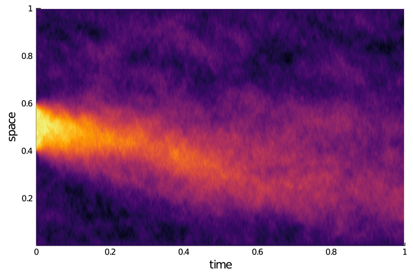
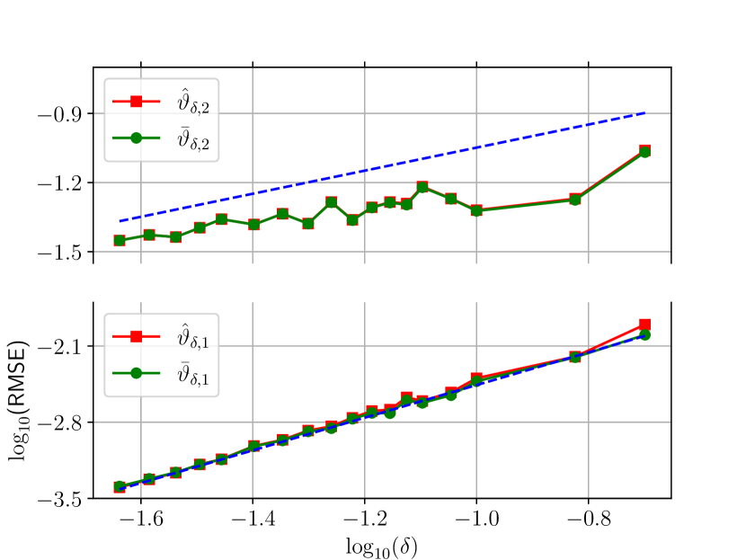
Figure 1: (left) heat map for a typical realisation of $X(t,x)$ corresponding to (1.1) in $d=1$ with domain $\Lambda=(0,1)$ in Example 5.1; (right) $\log_{10}\log_{10}$ plot of the root mean squared errors for estimating $\vartheta_{1}$ and $\vartheta_{2}$ in Example 5.1.

5.2 Statistical inference

The CLT in Theorem 2.3 easily yields statistical inference procedures. For instance, if $\alpha\in(0,1)$, $q_{1-\alpha}$ is the $1-\alpha$ quantile of the $\chi^{2}_{p}$-distribution and if $\lVert K\rVert_{L^{2}(\operatorname{{\mathbb{R}}}^{d})}=1$ for simplicity, then

$$C_{\alpha}=\{\vartheta\in\mathbb{R}^{p}:(\hat{\vartheta}_{\delta}-\vartheta)^{\top}\mathcal{I}_{\delta}(\hat{\vartheta}_{\delta}-\vartheta)\leq q_{1-\alpha}\}$$

is an asymptotic joint $1-\alpha$ confidence set for the parameter $\vartheta$.

Moreover, we can test for the presence of lower order terms. In Example 5.2, with the $1-\alpha$ quantile $z_{1-\alpha}$ of the standard normal distribution,

$$\phi_{\alpha}=\mathbf{1}\left(\left|\left(TM\delta^{2}/(2\hat{\vartheta}_{\delta,1})\lVert(-\Delta)^{-1/2}K\rVert^{2}_{L^{2}(\operatorname{{\mathbb{R}}}^{d})}\right)^{1/2}\hat{\vartheta}_{\delta,3}\right|>z_{1-\alpha}\right)$$

is an asymptotic level $\alpha$ test for testing the null hypothesis $H_{0}:\vartheta_{3}=0$ against the alternative $H_{1}:\vartheta_{3}<0$.

5.3 A boundary case: estimation in $d=2$

The augmented MLE generally does not satisfy the CLT in Theorem 2.3 in $d\leq 2$ for reaction terms $\vartheta_{i}$ with differential order $n_{i}=0$. We show now that in $d=2$ and for the maximal choice of measurements with $M=\lceil c\delta^{-2}\rceil$ the CLT can be recovered under integrability conditions on $K$, but consistency is lost, while for non-negative $K$ a logarithmic rate holds. This is consistent with results for the MLE from spectral observations in $d=2$, cf. [24]. For a proof see Section A.2.

Proposition 5.4.

Suppose that $d=2$, $A_{\vartheta}=\Delta+\vartheta$ for $\vartheta\in\operatorname{{\mathbb{R}}}$, $K\neq 0$, $X(0)=0$ and $M\delta^{2}\rightarrow 1$ as $\delta\rightarrow 0$. Then the following holds:

1. If $\int_{\operatorname{{\mathbb{R}}}^{2}}K(x)dx=0$, $\int_{\operatorname{{\mathbb{R}}}^{2}}xK(x)dx=0$, then $\hat{\vartheta}_{\delta}\stackrel{{\scriptstyle d}}{{\rightarrow}}\mathcal{N}(\vartheta,\lVert K\rVert^{2}_{L^{2}(\operatorname{{\mathbb{R}}}^{d})}\Sigma^{-1}_{\vartheta})$ with $\Sigma_{\vartheta}=(T/2)\lVert(-\Delta)^{-1/2}K\rVert_{L^{2}(\operatorname{{\mathbb{R}}}^{2})}^{2}$.

2. If $K\geq 0$, then $\hat{\vartheta}_{\delta}=\vartheta+O_{\operatorname{{\mathbb{P}}}}(\log(\delta^{-1})^{-1/2})$.

6 Proofs

Let us first define some notation. For convenience in the proofs we write the elliptic operator as $A_{\vartheta}=\nabla\cdot a_{\vartheta}\nabla+b_{\vartheta}\cdot\nabla+c_{\vartheta}$ with a symmetric positive definite matrix $a_{\vartheta}\in\operatorname{{\mathbb{R}}}^{d\times d}$, $b_{\vartheta}\in\operatorname{{\mathbb{R}}}^{d}$, $c_{\vartheta}\in\operatorname{{\mathbb{R}}}$ and let $\tilde{A}_{\vartheta}=\nabla\cdot a_{\vartheta}\nabla$. The operators $A_{\vartheta}$ and $\tilde{A}_{\vartheta}$ with domain $H^{1}_{0}(\Lambda)\cap H^{2}(\Lambda)$ generate the analytic semigroups $(S_{\vartheta}(t))_{t\geq 0}$ and $(\tilde{S}_{\vartheta}(t))_{t\geq 0}$. By a standard-PDE result (see, e.g., [27, Example III.6.11] or [39, equation (5.1)]) $A_{\vartheta}$ (and by [16, Example 2.1 in Section II.2]) its generated semigroup are diagonalizable, which yields the useful representations

$$A_{\vartheta}=U_{\vartheta}(\tilde{A}_{\vartheta}+\tilde{c}_{\vartheta})U_{\vartheta}^{-1},\quad S_{\vartheta}(t)=e^{t\tilde{c}_{\vartheta}}U_{\vartheta}\tilde{S}_{\vartheta}(t)U_{\vartheta}^{-1}$$ (6.1)

with the multiplication operator $(U_{\vartheta}z)(x)=\exp\left(-\frac{1}{2}(a_{\vartheta}^{-1}b_{\vartheta})\cdot x\right)z(x)$ and with $\tilde{c}_{\vartheta}=c_{\vartheta}-\frac{1}{4}b_{\vartheta}\cdot(a_{\vartheta}^{-1}b_{\vartheta})$. Below we will use $U_{\vartheta}$ to denote both the multiplication operator and the function $x\mapsto\exp\left(-\frac{1}{2}(a_{\vartheta}^{-1}b_{\vartheta})\cdot x\right)$.

6.1 The rescaled semigroup

In this section we collect a number of results on the semigroup operators $S_{\vartheta}(t)$ and their actions on localised functions $z_{\delta,x}(\cdot)=\delta^{-d/2}z(\delta^{-1}(\cdot-x))$. Write $\Lambda_{\delta,x}=\{\delta^{-1}(y-x):y\in\Lambda\}$, $\Lambda_{0,x}=\mathbb{R}^{d}$ and introduce the operators with domains $H_{0}^{1}(\Lambda_{\delta,x})\cap H^{2}(\Lambda_{\delta,x})$

$$A_{\vartheta,\delta,x} =\nabla\cdot a_{\vartheta}\nabla+\delta b_{\vartheta}\cdot\nabla+\delta^{2}c_{\vartheta},\quad\tilde{A}_{\vartheta,\delta,x}=\nabla\cdot a_{\vartheta}\nabla,$$ (6.2)

$$A_{i,\delta,x} =\delta^{n_{i}}\sum_{|\alpha|\leq n_{i}}\delta^{-|\alpha|}a^{(i)}_{\alpha}D^{\alpha}.$$

The operators in (6.2) generate the analytic semigroups $(S_{\vartheta,\delta,x}(t))_{t\geq 0}$ and $(\tilde{S}_{\vartheta,\delta,x}(t))_{t\geq 0}$ on $L^{2}(\Lambda_{\delta,x})$. Let $(\bar{S}_{\vartheta}(t))_{t\geq 0}$ be the semigroup on $L^{2}(\operatorname{{\mathbb{R}}}^{d})$ generated by $\bar{A}_{\vartheta}$. We also write $e^{t\Delta_{0}}=\bar{S}_{\vartheta}(t)$ when $a_{\vartheta}$ is the identity matrix.

Lemma 6.1.

Let $\delta^{\prime}\geq\delta\geq 0$, $x\in\Lambda$, $i=1,\dots,p$, $t\geq 0$.

1. If $z\in H_{0}^{1}(\Lambda_{\delta,x})\cap H^{2}(\Lambda_{\delta,x})$, then $A_{i}^{*}z_{\delta,x}=\delta^{-n_{i}}(A^{*}_{i,\delta,x}z)_{\delta,x}$, $A^{*}_{\vartheta}z_{\delta,x}=\delta^{-2}(A^{*}_{\vartheta,\delta,x}z)_{\delta,x}$.

2. If $z\in H^{2}(\operatorname{{\mathbb{R}}}^{d})$ is compactly supported in $\bigcap_{x\in\mathcal{J}}\Lambda_{\delta^{\prime},x}$, then $\sup_{x\in\mathcal{J}}\lVert A^{*}_{i,\delta,x}z-\bar{A}_{i}z\rVert_{L^{2}(\operatorname{{\mathbb{R}}}^{d})}\rightarrow 0$, $\sup_{x\in\mathcal{J}}\lVert A^{*}_{\vartheta,\delta,x}z-\bar{A}_{\vartheta}z\rVert_{L^{2}(\operatorname{{\mathbb{R}}}^{d})}\rightarrow 0$ as $\delta\rightarrow 0$.

3. If $z\in L^{2}(\Lambda_{\delta,x})$ then $S_{\vartheta}^{*}(t)z_{\delta,x}=(S_{\vartheta,\delta,x}^{*}(t\delta^{-2})z)_{\delta,x}$.

Proof.

Parts (i), (ii) are clear, part (iii) follows analogously to [4, Lemma 3.1]. ∎

The semigroup on the bounded domain $\Lambda_{\delta,x}$ is after zooming in as $\delta\rightarrow 0$ intuitively close to the semigroup on $\operatorname{{\mathbb{R}}}^{d}$. The next result states precisely in which way this holds, uniformly in $x\in\mathcal{J}$.

Lemma 6.2.

Under Assumption Assumption H(iii) the following holds:

• There exists $C>0$ such that if $z\in C_{c}(\mathbb{R}^{d})$ is supported in $\bigcap_{x\in\mathcal{J}}\Lambda_{\delta,x}$ for some $\delta\geq 0$, then for all $t\geq 0$

  $$\sup_{x\in\mathcal{J}}\left|(S^{*}_{\vartheta,\delta,x}(t)z)(y)\right|\leq Ce^{\tilde{c}_{\vartheta}t\delta^{2}}(\bar{S}_{\vartheta}(t)|z|)(y),\quad y\in\operatorname{{\mathbb{R}}}^{d}.$$

• If $z\in L^{2}(\mathbb{R}^{d})$, then as $\delta\rightarrow 0$ for all $t>0$

  $$\sup_{x\in\mathcal{J}}\mathop{}\!\mathbin{\lVert}S^{*}_{\vartheta,\delta,x}(t)(z|_{\Lambda_{\delta,x}})-\bar{S}_{\vartheta}(t)z\mathop{}\!\mathbin{\rVert}_{L^{2}(\mathbb{R}^{d})}\rightarrow 0.$$

Proof.

(i). Apply first the scaling in Lemma 6.1 in reverse order such that $(S^{*}_{\vartheta,\delta,x}(t)z)_{\delta,x}=S^{*}_{\vartheta}(t\delta^{2})z_{\delta,x}$. By (6.1) and direct computation, noting that the function $x\mapsto U_{\vartheta}(x)$ is uniformly upper and lower bounded on $\Lambda$, we get

$$|S^{*}_{\vartheta}(t\delta^{2})z_{\delta,x}| =|U_{\vartheta}^{-1}\tilde{S}_{\vartheta}(t\delta^{2})\exp(t\delta^{2}\tilde{c}_{\vartheta})U_{\vartheta}z_{\delta,x}|\lesssim e^{t\delta^{2}\tilde{c}_{\vartheta}}\tilde{S}_{\vartheta}(t\delta^{2})|z_{\delta,x}|.$$

Applying again the $\delta$-scaling it is therefore enough to prove the claim with respect to $\tilde{S}_{\vartheta}$ and with $|z|$ instead of $z$. By the classical Feynman-Kac formulas (cf. [26, Chapter 4.4], the anisotropic case is an easy generalisation, which can also be obtained by a change of variables leading to a diagonal diffusivity matrix $a_{\vartheta}$, which corresponds to $d$ scalar heat equations) we have with a process $Y_{t}=y+\mathop{}\!\mathbin{a}_{\vartheta}^{1/2}\tilde{W}_{t}$ and a $d$-dimensional Brownian motion $\tilde{W}$, all defined on another probability space with expectation and probability operators $\tilde{\operatorname{{\mathbb{E}}}}_{y}$, $\tilde{\operatorname{{\mathbb{P}}}}_{y}$, that $(\bar{S}_{\vartheta}(t)z)(y)=\tilde{\mathbb{E}}_{y}[z(Y_{t})]$ and $\tilde{S}_{\vartheta,\delta,x}(t)z(y)=\tilde{\mathbb{E}}_{y}\left[z(Y_{t})\mathbf{1}\left(t<\tau_{\delta,x}\right)\right]$ with the stopping times $\tau_{\delta,x}:=\inf\{t\geq 0:Y_{t}\notin\Lambda_{\delta,x}\}$. The claim follows now from

$$\sup_{x\in\mathcal{J}}(\tilde{S}_{\vartheta,\delta,x}(t)|z|)(y)\leq\tilde{E}_{y}[|z(Y_{t})|]=(\bar{S}_{\vartheta}(t)|z|)(y),$$

where the right hand side is $L^{2}(\operatorname{{\mathbb{R}}}^{d})$-integrable.

(ii). By an approximation argument it is enough to consider $z\in C_{c}(\bar{\Lambda})$ and $0<\delta\leq\delta^{\prime}$ such that $z$ is supported in $\Lambda_{\delta^{\prime},x}$, hence $z|_{\Lambda_{\delta,x}}=z$ for all such $\delta$. Compactness of $\mathcal{J}$ according to Assumption Assumption H(iii) guarantees for sufficiently small $\delta$ the existence of a ball $B_{\rho\delta^{-1}}\subset\bigcap_{x\in\mathcal{J}}\Lambda_{\delta,x}$ with center $0$ and radius $\rho\delta^{-1}$ for some $\rho>0$. With this and the representation formulas in (i), combined with the Cauchy-Schwarz inequality, we have for all $y\in\operatorname{{\mathbb{R}}}^{d}$

$$\sup_{x\in\mathcal{J}}|(\tilde{S}_{\vartheta,\delta,x}(t)z)(y)-(\bar{S}_{\vartheta}(t)z)(y)|^{2}=\sup_{x\in\mathcal{J}}|\tilde{\mathbb{E}}_{y}\left[z(Y_{t})\mathbf{1}(\tau_{\delta,x}\leq t)\right]|^{2}$$

$$\leq\sup_{x\in\mathcal{J}}\tilde{\operatorname{{\mathbb{E}}}}_{y}[z^{2}(Y_{t})]\tilde{\mathbb{P}}_{y}(\tau_{\delta,x}\leq t)\leq(\bar{S}_{\vartheta}(t)z^{2})(y)\tilde{\mathbb{P}}_{y}(\max_{0\leq s\leq t}|Y_{s}|\geq\rho\delta^{-1})$$

$$\leq(\bar{S}_{\vartheta}(t)z^{2})(y)\tilde{\mathbb{P}}_{y}(\max_{0\leq s\leq t}|\tilde{W}_{s}|\geq\tilde{\rho}\delta^{-1})\lesssim(\bar{S}_{\vartheta}(t)z^{2})(y)(\delta t^{1/2}e^{-\delta^{-2}t^{-1}})\rightarrow 0$$ (6.3)

as $\delta\rightarrow 0$ for a modified constant $\tilde{\rho}$, concluding by [26, equation (2.8.4)]. As a consequence of (6.1) and the $\delta$-scaling we have $(S^{*}_{\vartheta,\delta,x}(t)z)(y)=(U_{\vartheta,\delta,x}^{-1}\tilde{S}_{\vartheta,\delta,x}(t)e^{t\delta^{2}\tilde{c}_{\vartheta}}U_{\vartheta,\delta,x}z)(y)$ with $U_{\vartheta,\delta,x}z(y)=\exp(-(a_{\vartheta}^{-1}b_{\vartheta})\cdot(\delta y+x)/2)z(y)$. This converges to $z(y)$ uniformly in $x\in\mathcal{J}$ as $\delta\rightarrow 0$, and we also have $e^{t\delta^{2}\tilde{c}_{\vartheta}}\rightarrow 1$. With this conclude

$$\sup_{x\in\mathcal{J}}|(S^{*}_{\vartheta,\delta,x}(t)z)(y)-(\bar{S}_{\vartheta}(t)z)(y)|$$

$$=\sup_{x\in\mathcal{J}}|(U_{\vartheta,\delta,x}^{-1}\tilde{S}_{\vartheta,\delta,x}(t)e^{t\delta^{2}\tilde{c}_{\vartheta}}U_{\vartheta,\delta,x}z)(y)-(\bar{S}_{\vartheta}(t)z)(y)|\rightarrow 0,$$

by the uniform pointwise convergence in (6.3). From (i) we know that $\sup_{0\leq\delta\leq\delta^{\prime}}\sup_{x\in\mathcal{J}}|(S^{*}_{\vartheta,\delta,x}(t)z)(y)|$ is $L^{2}(\operatorname{{\mathbb{R}}}^{d})$-integrable. Dominated convergence yields the claim. ∎

We require frequently quantitative statements on the decay of the action of the semigroup operators $S^{*}_{\vartheta,\delta,x}(t)$ as $t\rightarrow\infty$ when applied to functions of a certain smoothness and integrability. This is well-known for a fixed general analytic semigroups, but is shown here to hold true regardless of $\delta$ and uniformly in $x\in\mathcal{J}$.

Lemma 6.3.

Let $0\leq\delta\leq 1$, $t>0$, $x\in\mathcal{J}$ and $1<p\leq\infty$. Moreover, let $z\in L^{p}(\Lambda_{\delta,x})$ if $1<p<\infty$ and $z\in C(\Lambda_{\delta,x})$ with $z=0$ on $\partial\Lambda_{\delta,x}$ if $p=\infty$. Then it holds with implied constants not depending on $x$:

$$\lVert A^{*}_{\vartheta,\delta,x}S^{*}_{\vartheta,\delta,x}(t)z\rVert_{L^{p}(\Lambda_{\delta,x})}\lesssim t^{-1}\lVert z\rVert_{L^{p}(\Lambda_{\delta,x})}.$$

Proof.

Apply first the scaling in Lemma 6.1 in reverse order such that with $1<p\leq\infty$

$$\lVert A^{*}_{\vartheta,\delta,x}S^{*}_{\vartheta,\delta,x}(t)z\rVert_{L^{p}(\Lambda_{\delta,x})}=\delta^{d(1/2-1/p)-2}\mathop{}\!\mathbin{\lVert}{A^{*}_{\vartheta}S^{*}_{\vartheta}(t\delta^{-2})z_{\delta,x}}\mathop{}\!\mathbin{\rVert}_{L^{p}(\Lambda)}.$$

If $p<\infty$, by the semigroup property for analytic semigroups in [5, Theorem V.2.1.3], the $L^{p}(\Lambda)$-norm is up to a constant upper bounded by $(t\delta^{-2})^{-1}\lVert z_{\delta,x}\rVert_{L^{p}(\Lambda)}$, and the claim follows. The same proof applies to $p=\infty$, noting that $A^{*}_{\vartheta}$ generates an analytic semigroup on $\{u\in C(\Lambda),u=0$ on $\partial\Lambda\}$, cf. [38, Theorem 7.3.7]. ∎

The proof for the next result relies on the Bessel-potential spaces $H_{0}^{s,p}(\Lambda_{\delta,x})$, $1<p<\infty$, $s\in\operatorname{{\mathbb{R}}}$, defined for $\delta>0$ as the domains of the fractional weighted Dirichlet-Laplacian $(-\tilde{A}_{\vartheta,\delta,x})^{s/2}$ of order $s/2$ on $\Lambda_{\delta,x}$ with norms $\lVert\cdot\rVert_{H^{s,p}(\Lambda_{\delta,x})}=\lVert(-\tilde{A}_{\vartheta,\delta,x})^{s/2}\cdot\rVert_{L^{p}(\Lambda_{\delta,x})}$, see [15] for details and also Section 6.4 below.

Lemma 6.4.

Let $0<\delta\leq 1$, $t>0$, $1<p\leq 2$ and grant Assumption Assumption H(iii). Let $z\in H_{0}^{s}(\mathbb{R}^{d})$, $s\geq 0$, be compactly supported in $\bigcap_{x\in\mathcal{J}}\Lambda_{\delta,x}$, suppose that $V_{\delta,x}:L^{p}(\Lambda_{\delta,x})\rightarrow H_{0}^{-s,p}(\Lambda_{\delta,x})$ are bounded linear operators with $\lVert V_{\delta,x}z\rVert_{H^{-s,p}(\Lambda_{\delta,x})}\leq V_{\operatorname{op}}\lVert z\rVert_{L^{p}(\Lambda_{\delta,x})}$ for some $V_{\operatorname{op}}$ independent of $\delta$, $x$. Then there exists a universal constant $C>0$ such that for $1<p\leq 2$ and $\gamma=(1/p-1/2)d/2$

$$\sup_{x\in\mathcal{J}}\mathop{}\!\mathbin{\lVert}S^{*}_{\vartheta,\delta,x}(t)V_{\delta,x}z\mathop{}\!\mathbin{\rVert}_{L^{2}(\Lambda_{\delta,x})} \leq Ce^{\tilde{c}_{\vartheta}t\delta^{2}}\sup_{x\in\mathcal{J}}\left(\lVert V_{\delta,x}z\rVert_{L^{2}(\Lambda_{\delta,x})}\wedge(V_{\operatorname{op}}t^{-s/2-\gamma}\lVert z\rVert_{L^{p}(\Lambda_{\delta,x})})\right).$$

If $s=0$, then this holds also for $p=1$.

Proof.

Let us write $u=V_{\delta,x}z$ and recall the multiplication operators $U_{\vartheta,\delta,x}$ from the proof of Proposition 6.2(ii). They are bounded operators on $L^{2}(\Lambda_{\delta,x})$ uniformly in $\delta\geq 0$ and $x\in\mathcal{J}$ and thus by (6.1)

$$\mathop{}\!\mathbin{\lVert}S^{*}_{\vartheta,\delta,x}(t)u\mathop{}\!\mathbin{\rVert}_{L^{2}(\Lambda_{\delta,x})} \lesssim e^{\tilde{c}_{\vartheta}t\delta^{2}}\mathop{}\!\mathbin{\lVert}\tilde{S}_{\vartheta,\delta,x}(t)U_{\vartheta,\delta,x}u\mathop{}\!\mathbin{\rVert}_{L^{2}(\Lambda_{\delta,x})}.$$ (6.4)

Let first $s=0$ such that $H_{0}^{-s,p}(\operatorname{{\mathbb{R}}}^{d})=L^{p}(\operatorname{{\mathbb{R}}}^{d})$. Approximating $u$ by continuous and compactly supported functions we obtain by Proposition 6.2(i), ellipticity of $a_{\vartheta}$ and hypercontractivity of the heat kernel on $\mathbb{R}^{d}$ uniformly in $x\in\mathcal{J}$

$$\mathop{}\!\mathbin{\lVert}S^{*}_{\vartheta,\delta,x}(t)u\mathop{}\!\mathbin{\rVert}_{L^{2}(\Lambda_{\delta,x})} \lesssim e^{\tilde{c}_{\vartheta}t\delta^{2}}\mathop{}\!\mathbin{\lVert}e^{Ct\Delta}|U_{\vartheta,\delta,x}u|\mathop{}\!\mathbin{\rVert}_{L^{2}(\operatorname{{\mathbb{R}}}^{d})}$$

$$\lesssim e^{\tilde{c}_{\vartheta}t\delta^{2}}t^{-\gamma}\lVert u\rVert_{L^{p}(\mathbb{R}^{d})}\lesssim e^{\tilde{c}_{\vartheta}t\delta^{2}}t^{-\gamma}\lVert z\rVert_{L^{p}(\operatorname{{\mathbb{R}}}^{d})}.$$

This yields the result for $s=0$. These inequalities hold also for $p=1$, thus proving the supplement of the statement. For $s>0$ and $p>1$ note first that by [3, Proposition 17(i)] we have $\lVert(-t\tilde{A}_{\vartheta,\delta,x})^{s/2}\tilde{S}_{\vartheta,\delta,x}(t)z\rVert_{L^{2}(\Lambda_{\delta,x})}\lesssim_{s}\lVert z\rVert_{L^{2}(\Lambda_{\delta,x})}$. Inserting this and then the last display with $u$ replaced by $(-\tilde{A}_{\vartheta,\delta,x})^{-s/2}U_{\vartheta,\delta,x}u$ into (6.4) we get

$$\mathop{}\!\mathbin{\lVert}S^{*}_{\vartheta,\delta,x}(t)u\mathop{}\!\mathbin{\rVert}_{L^{2}(\Lambda_{\delta,x})}\lesssim e^{\tilde{c}_{\vartheta}t\delta^{2}}\mathop{}\!\mathbin{\lVert}{(-\tilde{A}_{\vartheta,\delta,x})^{s/2}\tilde{S}_{\vartheta,\delta,x}(t)(-\tilde{A}_{\vartheta,\delta,x})^{-s/2}U_{\vartheta,\delta,x}u}\mathop{}\!\mathbin{\rVert}_{L^{2}(\Lambda_{\delta,x})}$$

$$\quad\lesssim e^{\tilde{c}_{\vartheta}t\delta^{2}}t^{-s/2}\mathop{}\!\mathbin{\lVert}{\tilde{S}_{\vartheta,\delta,x}(t/2)(-\tilde{A}_{\vartheta,\delta,x})^{-s/2}U_{\vartheta,\delta,x}u}\mathop{}\!\mathbin{\rVert}_{L^{2}(\Lambda_{\delta,x})}$$

$$\quad\lesssim e^{\tilde{c}_{\vartheta}t\delta^{2}}t^{-s/2-\gamma}\mathop{}\!\mathbin{\lVert}{U_{\vartheta,\delta,x}u}\mathop{}\!\mathbin{\rVert}_{H^{-s,p}(\Lambda_{\delta,x})},$$

uniformly in $x\in\mathcal{J}$. Since the functions $U_{\vartheta,\delta,x}$ are smooth and uniformly bounded on $\operatorname{{\mathbb{R}}}^{d}$ for $x\in\mathcal{J}$, they induce a family of multiplication operators on $H^{s,p}_{0}(\operatorname{{\mathbb{R}}}^{d})$ for $s\geq 0$ with operator norms uniformly bounded in $x\in\mathcal{J}$, cf. [45, Theorem 2.8.2]. By duality and restriction this transfers to $H^{s,p}_{0}(\Lambda_{\delta,x})$ for general $s$ according to [45, Theorem 3.3.2]. Hence,

$$\mathop{}\!\mathbin{\lVert}S^{*}_{\vartheta,\delta,x}(t)u\mathop{}\!\mathbin{\rVert}_{L^{2}(\Lambda_{\delta,x})}\lesssim e^{\tilde{c}_{\vartheta}t\delta^{2}}t^{-s/2-\gamma}\mathop{}\!\mathbin{\lVert}{u}\mathop{}\!\mathbin{\rVert}_{H^{-s,p}(\Lambda_{\delta,x})}\lesssim e^{\tilde{c}_{\vartheta}t\delta^{2}}t^{-s/2-\gamma}V_{\operatorname{op}}\lVert z\rVert_{L^{p}(\Lambda_{\delta,x})}.$$

∎

6.2 Proof of the central limit theorem

6.2.1 Covariance structure of multiple local measurements

Lemma 6.5.

1. If $X_{0}=0$, then the Gaussian process from (2.3) has mean zero and covariance function

   $$\operatorname{Cov}(\langle X(t),z\rangle,\langle X(t^{\prime}),z^{\prime}\rangle)=\int_{0}^{t\wedge t^{\prime}}\langle S^{*}_{\vartheta}(t-s)z,S^{*}_{\vartheta}(t^{\prime}-s)z^{\prime}\rangle ds.$$

2. If $X_{0}$ is the stationary initial condition from Lemma 2.2, then the Gaussian process from (2.3) has mean zero and covariance function

   $$\operatorname{Cov}(\langle X(t),z\rangle,\langle X(t^{\prime}),z^{\prime}\rangle)=\int_{0}^{\infty}\langle S^{*}_{\vartheta}(t+s)z,S^{*}_{\vartheta}(t^{\prime}+s)z^{\prime}\rangle ds.$$

Proof.

Part (i) follows from (2.2) and Itô’s isometry [14, Proposition 4.28]. For part (ii) we conclude in the same way from noting that the stationary solution given by $\langle X(t),z\rangle=\int_{-\infty}^{t}\langle S_{\vartheta}(t-s)z,dW(s)\rangle$ has mean zero. ∎

Lemma 6.6.

Grant Assumption Assumption H and let $X_{0}=0$. Introduce for $z,z^{\prime}\in L^{2}(\operatorname{{\mathbb{R}}}^{d})$

$$\Psi_{\vartheta}(z,z^{\prime}) =\int_{0}^{\infty}\langle\bar{S}_{\vartheta}(t^{\prime})z,\bar{S}_{\vartheta}(t^{\prime})z^{\prime}\rangle_{L^{2}(\operatorname{{\mathbb{R}}}^{d})}dt^{\prime}.$$

If $n_{i}+n_{j}>2-d$ for some $i,j=1,\dots,p$, then $\Psi_{\vartheta}(\bar{A}_{i}^{*}K,\bar{A}_{j}^{*}K)$ is well-defined and we have as $\delta\rightarrow 0$

$$\delta^{-2+n_{i}+n_{j}}(MT)^{-1}\sum_{k=1}^{M}\int_{0}^{T}\operatorname{{\mathbb{E}}}\left[\langle X(t),A_{i}^{*}K_{\delta,x_{k}}\rangle\langle X(t),A_{j}^{*}K_{\delta,x_{k}}\rangle\right]dt\rightarrow\Psi_{\vartheta}(\bar{A}_{i}^{*}K,\bar{A}_{j}^{*}K).$$

Proof.

Fix $i,j$ with $n_{i}+n_{j}>2-d$. Then, applying Lemma 6.5(i), the scaling from Lemma 6.1 and changing variables give

$$\delta^{-2+n_{i}+n_{j}}(MT)^{-1}\sum_{k=1}^{M}\int_{0}^{T}\operatorname{{\mathbb{E}}}\left[\langle X(t),A_{i}^{*}K_{\delta,x_{k}}\rangle\langle X(t),A_{j}^{*}K_{\delta,x_{k}}\rangle\right]dt=\int_{0}^{\infty}f_{\delta}(t^{\prime})dt^{\prime}$$

with

$$f_{\delta}(t^{\prime})=(MT)^{-1}\sum_{k=1}^{M}\langle S^{*}_{\vartheta,\delta,x_{k}}(t^{\prime})A^{*}_{i,\delta,x_{k}}K,S^{*}_{\vartheta,\delta,x_{k}}(t^{\prime})A^{*}_{j,\delta,x_{k}}K\rangle_{L^{2}(\Lambda_{\delta,x_{k}})}\int_{0}^{T}\mathbf{1}_{\{0\leq t^{\prime}\leq t\delta^{-2}\}}dt.$$

Consider now the differential operators $V_{\delta,x_{k}}=A^{*}_{i,\delta,x_{k}}$. If $D^{m}$ is a composition of $m$ partial differential operators, then Theorem 1.43 of [52] yields that $D^{m}$ is a bounded linear operator from $L^{p}(\Lambda)$ to $H_{0}^{-m,p}(\Lambda)$, implying $\mathop{}\!\mathbin{\lVert}{D^{m}K_{\delta,x_{k}}}\mathop{}\!\mathbin{\rVert}_{H^{-m,p}(\Lambda)}\lesssim\delta^{-m}\mathop{}\!\mathbin{\lVert}{K_{\delta,x_{k}}}\mathop{}\!\mathbin{\rVert}_{L^{p}(\Lambda)}$. Since $(D^{m}K)_{\delta,x_{k}}=\delta^{m}D^{m}K_{\delta,x_{k}}$, changing variables gives $\mathop{}\!\mathbin{\lVert}{D^{m}K}\mathop{}\!\mathbin{\rVert}_{H^{-m,p}(\Lambda_{\delta,x_{k}})}\lesssim\mathop{}\!\mathbin{\lVert}{K}\mathop{}\!\mathbin{\rVert}_{L^{p}(\Lambda_{\delta,x_{k}})}$. From this we find $\lVert V_{\delta,x_{k}}K\rVert_{H^{-n_{i},p}(\Lambda_{\delta,x})}\leq\lVert K\rVert_{L^{p}(\Lambda_{\delta,x_{k}})}$, $\lVert V_{\delta,x_{k}}K\rVert_{L^{2}(\Lambda_{\delta,x_{k}})}\lesssim\lVert K\rVert_{H^{n_{i}}(\operatorname{{\mathbb{R}}}^{d})}$, and Lemma 6.4 shows for $0\leq t^{\prime}\leq T\delta^{-2}$, $\varepsilon>0$ and all sufficiently small $\delta>0$

$$\sup_{x\in\mathcal{J}}\lVert S^{*}_{\vartheta,\delta,x}(t^{\prime})A^{*}_{i,\delta,x}K\rVert_{L^{2}(\Lambda_{\delta,x})}\lesssim 1\wedge(t^{\prime})^{-n_{i}/2-d/4+\varepsilon}.$$ (6.5)

This allows us to infer by the Cauchy-Schwarz inequality $|f_{\delta}(t^{\prime})|\lesssim 1\wedge(t^{\prime})^{-n_{i}/2-n_{j}/2-d/2+2\varepsilon}$. In particular, taking $\varepsilon$ so small that $n_{i}+n_{j}>2-d-4\varepsilon$ yields $\sup_{\delta>0}|f_{\delta}|\in L^{1}([0,\infty))$. Lemma 6.2(ii), Lemma 6.1(ii) and continuity of the $L^{2}$-scalar product show now pointwise for all $t^{\prime}>0$ that $f_{\delta}(t^{\prime})\rightarrow\langle\bar{S}_{\vartheta}(t^{\prime})\bar{A}^{*}_{i}K,\bar{S}_{\vartheta}(t^{\prime})\bar{A}^{*}_{j}K\rangle_{L^{2}(\operatorname{{\mathbb{R}}}^{d})}$. The wanted convergence follows from the dominated convergence theorem, which also shows that $\Psi_{\vartheta}(\bar{A}_{i}^{*}K,\bar{A}^{*}_{j}K)$ is well-defined. ∎

Lemma 6.7.

Grant Assumption Assumption H and let $X_{0}=0$. If $n_{i}+n_{j}>2-d$ for $i,j=1,\dots,p$, then $\sup_{x\in\mathcal{J}}\operatorname{Var}\left(\int_{0}^{T}\langle X(t),A^{*}_{i}K_{\delta,x}\rangle\langle X(t),A^{*}_{j}K_{\delta,x}\rangle dt\right)=o(\delta^{4-2n_{i}-2n_{j}})$.

Proof.

Applying the scaling from Lemma 6.1 and using Wicks theorem [25, Theorem 1.28] we have for $x\in\mathcal{J}$

$$\delta^{2n_{i}+2n_{j}}\operatorname{Var}\left(\int_{0}^{T}\langle X(t),A_{i}^{*}K_{\delta,x}\rangle\langle X(t),A_{j}^{*}K_{\delta,x}\rangle dt\right)$$

$$\quad=\operatorname{Var}\left(\int_{0}^{T}\langle X(t),(A^{*}_{i,\delta,x}K)_{\delta,x}\rangle\langle X(t),(A^{*}_{j,\delta,x}K)_{\delta,x}\rangle dt\right)=V_{1}+V_{2}$$

with

$$V_{1} =V_{\delta,x}(A^{*}_{i,\delta,x}K,A^{*}_{i,\delta,x}K,A^{*}_{j,\delta,x}K,A^{*}_{j,\delta,x}K),$$

$$V_{2} =V_{\delta,x}(A^{*}_{i,\delta,x}K,A^{*}_{j,\delta,x}K,A^{*}_{j,\delta,x}K,A^{*}_{i,\delta,x}K),$$

and where for $v,v^{\prime},z,z^{\prime}\in L^{2}(\Lambda_{\delta,x})$

$$V_{\delta,x}(v,v^{\prime},z,z^{\prime})=\int_{0}^{T}\int_{0}^{T}\operatorname{{\mathbb{E}}}[\langle X(t),v_{\delta,x}\rangle\langle X(t^{\prime}),v^{\prime}_{\delta,x}\rangle]\operatorname{{\mathbb{E}}}[\langle X(t),z_{\delta,x}\rangle\langle X(t^{\prime}),z^{\prime}_{\delta,x}\rangle]dt^{\prime}dt.$$

We only upper bound $V_{1}$, the arguments for $V_{2}$ are similar. Set $f_{i,j}(s,s^{\prime})=\langle S^{*}_{\vartheta,\delta,x}(s+s^{\prime})A^{*}_{i,\delta,x}K,S^{*}_{\vartheta,\delta,x}(s^{\prime})A^{*}_{j,\delta,x}K\rangle_{L^{2}(\Lambda_{\delta,x})}$. Using Lemma 6.5(i) and the scaling from Lemma 6.1 we have

$$V_{1}=2\delta^{6}\int_{0}^{T}\int_{0}^{t\delta^{-2}} \left(\int_{0}^{t\delta^{-2}-s}f_{i,i}(s,s^{\prime})ds^{\prime}\right)\left(\int_{0}^{t\delta^{-2}-s}f_{j,j}(s,s^{\prime\prime})ds^{\prime\prime}\right)dsdt,$$

cf. [4, Proof of Proposition A.9]. From (6.5) and the Cauchy-Schwarz inequality we infer for $\varepsilon>0$

$$\sup_{x\in\mathcal{J}}\left|f_{i,i}(s,s^{\prime})f_{j,j}(s,s^{\prime\prime})\right|\lesssim \left(1\wedge s^{-n_{i}/2-n_{j}/2-d/2+2\varepsilon}\right)\left(1\wedge s^{\prime-n_{i}/2-d/4+\varepsilon}\right)$$

$$\quad\cdot\left(1\wedge s^{\prime\prime-n_{j}/2-d/4+\varepsilon}\right),$$

which gives

$$\sup_{x\in\mathcal{J}}\left|V_{1}\right| \lesssim\delta^{6}\int_{0}^{T\delta^{-2}}\left(1\wedge s^{-n_{i}/2-n_{j}/2-d/2+2\varepsilon}\right)ds\int_{0}^{T\delta^{-2}}\left(1\wedge s^{\prime-n_{i}/2-d/4+\varepsilon}\right)ds^{\prime}$$

$$\quad\quad\cdot\int_{0}^{T\delta^{-2}}\left(1\wedge s^{\prime\prime-n_{j}/2-d/4+\varepsilon}\right)ds^{\prime\prime}$$

$$\lesssim\delta^{6}\left(1\vee\delta^{n_{i}+n_{j}+d-2-4\varepsilon}\right)\left(1\vee\delta^{n_{i}+d/2-2-2\varepsilon}\right)\left(1\vee\delta^{n_{j}+d/2-2-2\varepsilon}\right).$$

Without loss of generality let $n_{i}\leq n_{j}$. Taking $\varepsilon$ small enough, we can ensure $1\vee\delta^{n_{i}+n_{j}+d-2-4\varepsilon}=1$, as $n_{i}+n_{j}>2-d$. In $d\leq 2$ only the pairs $(n_{i},n_{j})\in\{(0,0),(0,1)\}$ are excluded, and in every case the claimed bound holds. The same applies to $d\geq 3$ for all pairs $(n_{i},n_{j})$. ∎

6.2.2 Proof of Theorem 2.3

Proof.

We begin with the observed Fisher information. Suppose first $X_{0}=0$. Under Assumption Assumption H we find that $n_{i}+n_{j}>2-d$ for all $i,j=1,\dots,p$ in all dimensions $d\geq 1$. It follows from Lemmas 6.6 and 6.7 that

$$(\rho_{\delta}\mathcal{I}_{\delta}\rho_{\delta})_{ij} =\delta^{-2+n_{i}+n_{j}}M^{-1}\sum_{k=1}^{M}\int_{0}^{T}\langle X(t),A_{i}^{*}K_{\delta,x_{k}}\rangle\langle X(t),A_{j}^{*}K_{\delta,x_{k}}\rangle dt$$

$$=T\Psi_{\vartheta}(\bar{A}^{*}_{i}K,\bar{A}^{*}_{j}K)+o_{\operatorname{{\mathbb{P}}}}(1)=(\Sigma_{\vartheta})_{ij}+o_{\operatorname{{\mathbb{P}}}}(1),$$

concluding by $\Psi_{\vartheta}(z,z^{\prime})=\frac{1}{2}\langle(-\bar{A}_{\vartheta})^{-1/2}z,(-\bar{A}_{\vartheta})^{-1/2}z^{\prime}\rangle_{L^{2}(\operatorname{{\mathbb{R}}}^{d})}$. This yields for $X_{0}=0$ the wanted convergence

$$\rho_{\delta}\mathcal{I}_{\delta}\rho_{\delta}\stackrel{{\scriptstyle\operatorname{{\mathbb{P}}}}}{{\rightarrow}}\Sigma_{\vartheta}.$$ (6.6)

In order to extend this to the general $X_{0}$ from Assumption Assumption H, let $\bar{X}$ be defined as $X$, but starting in $\bar{X}(0)=0$ such that for $v\in L^{2}(\Lambda)$, $\langle X(t),v\rangle=\langle\bar{X}(t),v\rangle+\langle S_{\vartheta}(t)X_{0},v\rangle$. If $\bar{\mathcal{I}}_{\delta}$ is the observed Fisher information corresponding to $\bar{X}$, then by the Cauchy-Schwarz inequality, with $v_{i}=\sup_{k}\delta^{2n_{i}-2}\int_{0}^{T}\langle X_{0},S^{*}_{\vartheta}(t)A^{*}_{i}K_{\delta,x_{k}}\rangle^{2}dt$,

$$|(\rho_{\delta}\mathcal{I}_{\delta}\rho_{\delta})_{ij}-(\rho_{\delta}\bar{\mathcal{I}}_{\delta}\rho_{\delta})_{ij}|\lesssim(\rho_{\delta}\bar{\mathcal{I}}_{\delta}\rho_{\delta})_{ii}^{1/2}v_{j}^{1/2}+(\rho_{\delta}\bar{\mathcal{I}}_{\delta}\rho_{\delta})_{jj}^{1/2}v_{i}^{1/2}+v_{i}^{1/2}v_{j}^{1/2}.$$

By the first part, $(\rho_{\delta}\bar{\mathcal{I}}_{\delta}\rho_{\delta})_{ii}$ is bounded in probability and Assumption Assumption H(iv) gives $v_{i}=o_{\operatorname{{\mathbb{P}}}}(1)$ for all $i$. From this obtain again (6.6).

Regarding the invertibility of $\Sigma_{\vartheta}$, let $\lambda\in\operatorname{{\mathbb{R}}}^{p}$ such that

$$0=\sum_{i,j=1}^{p}\lambda_{i}\lambda_{j}(\Sigma_{\vartheta})_{ij} =T\Psi_{\vartheta}\left(\sum_{i=1}^{p}\lambda_{i}\bar{A}^{*}_{i}K,\sum_{i=1}^{p}\lambda_{i}\bar{A}^{*}_{i}K\right).$$

By the definition of $\Psi_{\vartheta}$ this implies $\bar{S}_{\vartheta}(t)(\sum_{i=1}^{p}\lambda_{i}\bar{A}^{*}_{i}K)=0$ for all $t\geq 0$ and thus $\sum_{i=1}^{p}\lambda_{i}\bar{A}^{*}_{i}K=0$. Since the functions $\bar{A}^{*}_{i}K$ are linearly independent by Assumption Assumption H(i), conclude that $\Sigma_{\vartheta}$ is invertible.

We proceed next to the proof of the CLT. The augmented MLE and the statement of the limit theorem remain unchanged when $K$ is multiplied by a scalar factor. We can therefore assume without loss of generality that $\lVert K\rVert_{L^{2}(\operatorname{{\mathbb{R}}}^{d})}=1$. By the basic error decomposition (2.8) and because $\Sigma_{\vartheta}$ is invertible, this means

$$(\rho_{\delta}\mathcal{I}_{\delta}\rho_{\delta})^{1/2}\rho_{\delta}^{-1}(\hat{\vartheta}_{\delta}-\vartheta)=(\rho_{\delta}\mathcal{I}_{\delta}\rho_{\delta})^{-1/2}\Sigma_{\vartheta}^{1/2}(\Sigma_{\vartheta}^{-1/2}\rho_{\delta}\mathcal{M}_{\delta}).$$ (6.7)

Note that $\mathcal{M}_{\delta}=\mathcal{M}_{\delta}(T)$ corresponds to a $p$-dimensional continuous and square integrable martingale $(\mathcal{M}_{\delta}(t))_{0\leq t\leq T}$ with respect to the filtration $(\mathcal{F}_{t})_{0\leq t\leq T}$ evaluated at $t=T$. In view of the support Assumption Assumption H(i) let $\delta\leq\delta^{\prime}$ such that for $k,k^{\prime}$ with the Kronecker delta $\delta_{k,k^{\prime}}$

$$\operatorname{{\mathbb{E}}}[W_{k}(t)W_{k^{\prime}}(t)]=\operatorname{{\mathbb{E}}}[\langle W(t),K_{\delta,x_{k}}\rangle\langle W(t),K_{\delta,x_{k^{\prime}}}\rangle]=\langle K_{\delta,x_{k}},K_{\delta,x_{k^{\prime}}}\rangle=\delta_{k,k^{\prime}}.$$

This means that the Brownian motions $W_{k}$ and $W_{k^{\prime}}$ are independent for $k\neq k^{\prime}$ and thus their quadratic co-variation process at $t$ is $[W_{k},W_{k^{\prime}}]=t\delta_{k,k^{\prime}}$. From this infer that the quadratic co-variation process of the martingale $(\mathcal{M}_{\delta}(t))_{0\leq t\leq T}$ at $t=T$ for $\delta\leq\delta^{\prime}$ is equal to

$$[\mathcal{M}_{\delta}]_{T}=\sum_{k,k^{\prime}=1}^{M}\int_{0}^{T}X^{A}_{\delta,k}(t)X^{A}_{\delta,k^{\prime}}(t)d[W_{k},W_{k^{\prime}}]_{t}=\mathcal{I}_{\delta}.$$

Theorem A.1 now implies $\Sigma_{\vartheta}^{-1/2}\rho_{\delta}\mathcal{M}_{\delta}\stackrel{{\scriptstyle d}}{{\rightarrow}}\mathcal{N}(0,I_{p})$. Conclude in (6.7) by (6.6) and Slutsky’s lemma. ∎

6.3 Proof of Theorem 3.1

In this section, we give the main steps of the proof of Theorem 3.1. The RKHS computations and the proofs of two key lemmas are deferred to Section 6.4 and the appendix.

6.3.1 Gaussian minimax lower bounds

Let $(\mathbb{P}_{\vartheta})_{\vartheta\in\Theta}$ be a family of probability measures defined on the same measurable space with a parameter set $\Theta\subseteq\mathbb{R}^{p}$. For $\vartheta^{0},\vartheta^{1}\in\Theta$, the (squared) Hellinger distance between $\mathbb{P}_{\vartheta^{0}}$ and $\mathbb{P}_{\vartheta^{1}}$ is defined by $H^{2}(\mathbb{P}_{\vartheta^{0}},\mathbb{P}_{\vartheta^{1}})=\int(\sqrt{\mathbb{P}_{\vartheta^{0}}}-\sqrt{\mathbb{P}_{\vartheta^{1}}})^{2}$ (see, e.g. [46, Definition 2.3]). Moreover, if $\vartheta^{0},\vartheta^{1}\in\Theta$ satisfy

$$\ H^{2}(\mathbb{P}_{\vartheta^{0}},\mathbb{P}_{\vartheta^{1}})\leq 1,$$ (6.8)

then we have the lower bound

$$\inf_{\hat{\vartheta}}\max_{\vartheta\in\{\vartheta^{0},\vartheta^{1}\}}\mathbb{P}_{\vartheta}\left(|\hat{\vartheta}-\vartheta|\geq\frac{|\vartheta^{0}-\vartheta^{1}|}{2}\right)\geq\frac{1}{4}\frac{2-\sqrt{3}}{4}=:c_{3},$$ (6.9)

where the infimum is taken over all $\operatorname{{\mathbb{R}}}^{p}$-valued estimators $\hat{\vartheta}$ and $|\cdot|$ denotes the Euclidean norm. For a proof of this lower bound, see [46, Theorem 2.2(ii)].

Next, let $\mathbb{P}_{\vartheta^{0}}$ and $\mathbb{P}_{\vartheta^{1}}$ be two Gaussian measures defined on a separable Hilbert space $\mathcal{H}$ with expectation zero and positive self-adjoint trace-class covariance operators $C_{\vartheta^{0}}$ and $C_{\vartheta^{1}}$, respectively. By the spectral theorem, there exist (strictly) positive eigenvalues $(\sigma_{j}^{2})_{j\geq 1}$ and an associated orthonormal system of eigenvectors $(u_{j})_{j\geq 1}$ such that $C_{\vartheta^{0}}=\sum_{j\geq 1}\sigma_{j}^{2}(u_{j}\otimes u_{j})$. Given the Gaussian measure $\mathbb{P}_{\vartheta^{0}}$, we can associate the so-called kernel or RKHS $(H_{\vartheta^{0}},\|\cdot\|_{H_{\vartheta^{0}}})$ of $\mathbb{P}_{\vartheta^{0}}$ given by

$$H_{\vartheta^{0}}=\{h\in\mathcal{H}:\|h\|_{H_{\vartheta^{0}}}<\infty\},\qquad\|h\|_{H_{\vartheta^{0}}}^{2}=\sum_{j\geq 1}\frac{\langle u_{j},h\rangle_{\mathcal{H}}^{2}}{\sigma_{j}^{2}}$$ (6.10)

(see, e.g., [32, Example 4.2] and also [32, Chapters 4.1 and 4.3] and [19, Chapter 3.6] for other characterizations of the RKHS of a Gaussian measure or process). Alternatively, we have $H_{\vartheta^{0}}=C_{\vartheta^{0}}^{1/2}\mathcal{H}$ and $\|h\|_{H_{\vartheta^{0}}}=\lVert C_{\vartheta^{0}}^{-1/2}h\rVert$ for $h\in H_{\vartheta^{0}}$. A useful tool to compute the RKHS is the fact that the RKHS behaves well under linear transformation. More precisely, if $L:\mathcal{H}\rightarrow\mathcal{H}^{\prime}$ is a bounded linear operator between Hilbert spaces, then the image measure $Q_{\vartheta^{0}}=\mathbb{P}_{\vartheta^{0}}\circ L^{-1}$ is a centered Gaussian measure having RKHS $L(H_{\vartheta^{0}})$ with norm $\lVert h\rVert_{L(H_{\vartheta^{0}})}=\inf\{\lVert f\rVert_{\mathcal{H}}:f\in L^{-1}h\}$ (see Proposition 4.1 in [32] and also Chapter 3.6 in [19]).

Finally, combining (6.8) with the RKHS machinery, we get the following lower bound.

Lemma 6.8.

In the above Gaussian setting, suppose that $(u_{j})_{j\geq 1}$ is an orthonormal basis of $\mathcal{H}$ and that

$$\sum_{j\geq 1}\sigma_{j}^{-2}\|(C_{\vartheta^{1}}-C_{\vartheta^{0}})u_{j}\|_{H_{\vartheta^{0}}}^{2}\leq 1/2.$$ (6.11)

Then the lower bound in (6.9) holds, that is

$$\inf_{\hat{\vartheta}}\max_{\vartheta\in\{\vartheta^{0},\vartheta^{1}\}}\mathbb{P}_{\vartheta}\left(|\hat{\vartheta}-\vartheta|\geq\frac{|\vartheta^{0}-\vartheta^{1}|}{2}\right)\geq c_{3}.$$

Lemma 6.8 is a consequence of the proof of the Feldman-Hajek theorem [14, Theorem 2.25] in combination with basic properties of the Hellinger distance and the minimax risk. A proof is given in Appendix A.3.

6.3.2 Proof of Theorem 3.1

Our goal is to apply Lemma 6.8 and Corollary 4.3 to the Gaussian process $X_{\delta}$ under Assumption Assumption L. We assume without loss of generality that $\lVert K\rVert_{L^{2}(\operatorname{{\mathbb{R}}}^{d})}=1$. We choose $\vartheta^{0}=(1,0,0)$ and $\vartheta^{1}\in\Theta_{1}\cup\Theta_{2}\cup\Theta_{3}$, meaning that the null model is $A_{\vartheta^{0}}=\Delta$ and the alternatives are $A_{\vartheta^{1}}=\vartheta^{1}_{1}\Delta+\vartheta^{1}_{2}(b\cdot\nabla)+\vartheta^{1}_{3}$ for $\vartheta^{1}\in\operatorname{{\mathbb{R}}}^{3}$, where $\vartheta^{1}$ lies in one of the parameter classes $\Theta_{1}$, $\Theta_{2}$ or $\Theta_{3}$. For $\vartheta\in\{\vartheta^{0},\vartheta^{1}\}$, let $\operatorname{{\mathbb{P}}}_{\vartheta,\delta}$ be the law of $X_{\delta}$ on $\mathcal{H}=L^{2}([0,T])^{M}$, let $C_{\vartheta,\delta}$ be its covariance operator, and let $(H_{\vartheta,\delta},\lVert\cdot\rVert_{H_{\vartheta,\delta}})$ be the associated RKHS. For $(f_{k})_{k=1}^{M}\in\mathcal{H}$, we have $C_{\vartheta,\delta}(f_{k})_{k=1}^{M}=(\sum_{l=1}^{M}C_{\vartheta,\delta,k,l}f_{l})_{k=1}^{M}$ with (cross-)covariance operators defined by

$$C_{\vartheta,\delta,k,l}:L^{2}([0,T])\rightarrow L^{2}([0,T]),$$

$$C_{\vartheta,\delta,k,l}f_{l}(t)=\operatorname{{\mathbb{E}}}_{\vartheta}[\langle X_{\delta,l},f_{l}\rangle_{L^{2}([0,T])}X_{\delta,k}(t)],\qquad 0\leq t\leq T$$

(see, e.g., Appendix A.4 for more background on bounded linear operator on $\mathcal{H}$). Because of the stationary of $X_{\delta}$ under Assumption Assumption L, we have

$$C_{\vartheta,\delta,k,l}f_{l}(t) =\int_{0}^{t}c_{\vartheta,\delta,k,l}(t-t^{\prime})f_{l}(t^{\prime})\,dt^{\prime}+\int_{t}^{T}c_{\vartheta,\delta,l,k}(t^{\prime}-t)f_{l}(t^{\prime})\,dt^{\prime},\quad 0\leq t\leq T$$

with covariance kernels

$$c_{\vartheta,\delta,k,l}(t)=\operatorname{{\mathbb{E}}}_{\vartheta}[X_{\delta,k}(t)X_{\delta,l}(0)],\qquad 0\leq t\leq T.$$

Following the notation of Section 6.3.1, let $(\sigma_{j}^{2})_{j\geq 1}$ be the strictly positive eigenvalues of $C_{\vartheta^{0},\delta}$ and let $(u_{j})_{j\geq 1}$ with $u_{j}=(u_{j,k})_{k=1}^{m}\in\mathcal{H}$ be a corresponding orthonormal system of eigenvectors. By Corollary 4.3, we have $H_{\vartheta^{0},\delta}=H^{M}$ as sets. Since $H^{M}$ is dense in $\mathcal{H}$, $(u_{j})_{j\geq 1}$ forms an orthonormal basis of $\mathcal{H}$. This means that the first assumption of Lemma 6.8 is satisfied. To verify the second assumption in (6.11), we will use the bound for the RKHS norm in Corollary 4.3 to turn the left-hand side of (6.11) into a more accessible expression.

Lemma 6.9.

In the above setting, we have

$$\sum_{j=1}^{\infty}\sigma_{j}^{-2}\lVert(C_{\vartheta^{0},\delta}-C_{\vartheta^{1},\delta})u_{j}\rVert^{2}_{H_{\vartheta^{0},\delta}}$$

$$\leq cT\sum_{k,l=1}^{M}\Big{(}\frac{\lVert\Delta K\rVert^{4}_{L^{2}(\operatorname{{\mathbb{R}}}^{d})}}{\delta^{8}}\lVert c_{\vartheta^{0},\delta,k,l}-c_{\vartheta^{1},\delta,k,l}\rVert^{2}_{L^{2}([0,T])}+\lVert c_{\vartheta^{0},\delta,k,l}^{\prime\prime}-c_{\vartheta^{1},\delta,k,l}^{\prime\prime}\rVert^{2}_{L^{2}([0,T])}\Big{)}$$

for all $\delta^{2}\leq\lVert\Delta K\rVert_{L^{2}(\operatorname{{\mathbb{R}}}^{d})}$ and all $T\geq 1$, where $c>0$ is an absolute constant.

The proof of Lemma 6.9 can be found in Appendix A.4. Moreover, combining Lemma 6.5(ii) with perturbation arguments for semigroups, we prove the following upper bound in Section A.5.

Lemma 6.10.

In the above setting let $\vartheta^{1}=(\vartheta_{1},\vartheta_{2},\vartheta_{3})\in\Theta_{1}\cup\Theta_{2}\cup\Theta_{3}$ with $M\geq 1$. Then there exists a constant $c>0$, depending only on $K$ such that

$$\sum_{k,l=1}^{M}\left(\delta^{-8}\lVert c_{\vartheta^{0},\delta,k,l}-c_{\vartheta^{1},\delta,k,l}\rVert^{2}_{L^{2}([0,T])}+\lVert c_{\vartheta^{0},\delta,k,l}^{\prime\prime}-c_{\vartheta^{1},\delta,k,l}^{\prime\prime}\rVert^{2}_{L^{2}([0,T])}\right)$$

$$\qquad\leq cM(\delta^{-2}(1-\vartheta_{1})^{2}+\vartheta_{2}^{2}+\delta^{2}\vartheta_{3}^{2}).$$

Choosing consecutively

$$\vartheta^{1} =(\vartheta_{1},0,0)\in\Theta_{1},\qquad\vartheta_{1}=1+c_{2}\frac{\delta}{\sqrt{TM}},$$

$$\vartheta^{1} =(1,\vartheta_{2},0)\in\Theta_{2},\qquad\vartheta_{2}=c_{2}\frac{1}{\sqrt{TM}},$$

$$\vartheta^{1} =(1,0,\vartheta_{3})\in\Theta_{3},\qquad\vartheta_{3}=c_{2}\min\Big{(}1,\frac{\delta^{-1}}{\sqrt{TM}}\Big{)},$$

claims (i) and (ii) of Theorem 3.1 follow from Lemma 6.8 in combination with Lemmas 6.9 and 6.10. ∎

6.4 RKHS computations

The proofs of the RKHS results from Section 4 are achieved by basic operations on RKHS, in particular under linear transformation (see, e.g., Section 6.3.1 and [32, Chapter 4] or [49, Chapter 12]).

Recall the stationary process $X$ in (4.1) and that $A_{\vartheta}e_{j}=-\lambda_{j}e_{j}$. The cylindrical Wiener process can be realised as $W=\sum_{j\geq 1}e_{j}\beta_{j}$ for independent scalar Brownian motions $\beta_{j}$ and we obtain the decomposition

$$X(t)=\sum_{j\geq 1}\int_{-\infty}^{t}e^{-\lambda_{j}(t-t^{\prime})}d\beta_{j}(t^{\prime})e_{j}=\sum_{j\geq 1}Y_{j}(t)e_{j},$$ (6.12)

with independent stationary Ornstein-Uhlenbeck processes $Y_{j}$ satisfying

$$dY_{j}(t)=-\lambda_{j}Y_{j}(t)dt+d\beta_{j}(t).$$ (6.13)

For a sequence $(\mu_{j})$ of non-decreasing, positive real numbers, take $\mathcal{H}_{1}$ to be the closure of $\mathcal{H}$ under the norm

$$\lVert z\rVert^{2}_{\mathcal{H}_{1}}=\sum_{j\geq 1}\frac{1}{\mu_{j}^{2}}\langle z,e_{j}\rangle^{2}_{\mathcal{H}},$$

such that $\mathcal{H}$ is continuously embedded in $\mathcal{H}_{1}$. If for $0\leq t\leq T$

$$\int_{-\infty}^{t}\lVert S_{\vartheta}(t^{\prime})\rVert^{2}_{\operatorname{HS}(\mathcal{H},\mathcal{H}_{1})}dt^{\prime} =\sum_{j\geq 1}\int_{-\infty}^{t}\lVert S_{\vartheta}(t^{\prime})e_{j}\rVert^{2}_{\mathcal{H}_{1}}dt^{\prime}$$

$$=\sum_{j\geq 1}\frac{1}{\mu_{j}^{2}}\int_{-\infty}^{t}e^{-2\lambda_{j}t^{\prime}}dt^{\prime}<\infty,$$ (6.14)

then we conclude by [14, Theorem 5.2] that the law of $X$ induces a Gaussian measure on $L^{2}([0,T];\mathcal{H}_{1})$. A first universal choice is given by $\mu_{j}=j$ for all $j\geq 1$. Moreover, if $A_{\vartheta}$ is a differential operator, then Weyl’s law [42, Lemma 2.3] says that the $\lambda_{j}$ are positive real numbers of the order $j^{2/d}$, meaning that the choice $\mu_{j}=\lambda_{j}^{s/2}$ is possible whenever $s\geq 0$ and $s+1>d/2$. In this case, $\mathcal{H}_{1}$ corresponds to a Sobolev space of negative order $-s$ induced by the eigensequence $(\lambda_{j},e_{j})_{j\geq 1}$.

6.4.1 RKHS of an Ornstein-Uhlenbeck process

We start by computing the RKHS $(H_{Y_{j}},\lVert\cdot\rVert_{Y_{j}})$ of the processes $Y_{j}$. We show that the RKHS is, as a set, independent of $j$ and equal to

$$H=\{h\in L^{2}([0,T]):h\text{ absolutely continuous},h^{\prime}\in L^{2}([0,T])\}$$

from Theorem 4.2, while the corresponding norm depends on the parameter $\lambda_{j}$.

Lemma 6.11.

For every $j\geq 1$ we have $H_{Y_{j}}=H$ and

$$\lVert h\rVert^{2}_{Y_{j}} =\lambda_{j}^{2}\lVert h\rVert^{2}_{L^{2}([0,T])}+\lambda_{j}(h^{2}(T)+h^{2}(0))+\lVert h^{\prime}\rVert^{2}_{L^{2}([0,T])}.$$ (6.15)

Proof.

By Example 4.4 in [32], a scalar Brownian motion $(\beta(t))_{0\leq t\leq T}$ starting in zero has RKHS $H_{\beta}=\{h:h(0)=0,h\text{ absolutely continuous, }h,h^{\prime}\in L^{2}([0,T])\}$ with norm $\lVert h\rVert_{H_{\beta}}^{2}=\int_{0}^{T}(h^{\prime}(t))^{2}\,dt$. Moreover, the Brownian motion $(\bar{\beta}(t))_{0\leq t\leq T}$ with $\bar{\beta}(t)=X_{0}+\beta(t)$, where $X_{0}$ is a standard Gaussian random variable independent of $(\beta(t))_{0\leq t\leq T}$ has RKHS

$$H_{\bar{\beta}}=\{\alpha+h:\alpha\in\operatorname{{\mathbb{R}}},h\in H_{\beta}\}=H,\quad\lVert h\rVert_{H_{\bar{\beta}}}^{2}=\int_{0}^{T}(h^{\prime}(t))^{2}\,dt+h^{2}(0),$$

as can be seen from Proposition 4.1 in [32] or Example 12.28 in [49]. To compute the RKHS of $Y_{j}$ we now proceed similarly as in Example 4.8 in [32]. Define the bounded linear map $L:L^{2}([0,e^{2\lambda_{j}T}-1])\rightarrow L^{2}([0,T])$, $(Lf)(t)=(2\lambda_{j})^{-1/2}e^{-\lambda_{j}t}f(e^{2\lambda_{j}t}-1)$. Then we have $L\bar{\beta}=Y_{j}$ in distribution and $L$ is bijective with inverse $L^{-1}h(s)=\sqrt{2\lambda_{j}(s+1)}h((2\lambda_{j})^{-1}\log(s+1))$, $0\leq s\leq e^{2\lambda_{j}T}-1$. By Proposition 4.1 in [32] (see also the discussion after (6.10)), we conclude that $H_{Y_{j}}=L(H_{\bar{\beta}})=L(H)=H$ with

$$\|h\|_{Y_{j}}^{2} =\|L^{-1}h\|_{H_{\bar{\beta}}}^{2}$$

$$=\int_{0}^{e^{2\lambda_{j}T}-1}\Big{(}\frac{d}{ds}\sqrt{2\lambda_{j}(s+1)}h\Big{(}\frac{1}{2\lambda_{j}}\log(s+1)\Big{)}\Big{)}^{2}\,ds+2\lambda_{j}h^{2}(0)$$

$$=\int_{0}^{T}(\lambda_{j}h(t)+h^{\prime}(t))^{2}\,dt+2\lambda_{j}h^{2}(0)$$

$$=\lambda_{j}^{2}\int_{0}^{T}h^{2}(t)\,dt+\lambda_{j}(h^{2}(T)+h^{2}(0))+\int_{0}^{T}(h^{\prime}(t))^{2}\,dt.$$

This completes the proof. ∎

6.4.2 RKHS of the SPDE

We compute next the RKHS of the process $X$. Let us start with the following series representation, which is independent of $\mathcal{H}_{1}$.

Lemma 6.12.

The RKHS $(H_{X},\|\cdot\|_{X})$ of the process $X$ in (4.1) satisfies

$$H_{X}=\Big{\{}h=\sum_{j\geq 1}h_{j}e_{j}:h_{j}\in H,\|h\|_{X}<\infty\Big{\}}\quad\text{and}\quad\|h\|_{X}^{2}=\sum_{j\geq 1}\|h_{j}\|_{Y_{j}}^{2}.$$

Proof.

For simplicity, choose $\mu_{j}=j$ for all $j\geq 1$. Since $X(t)=\sum_{j\geq 1}j^{-1}Y_{j}(t)\tilde{e}_{j}$ with orthonormal basis $\tilde{e}_{j}=je_{j}$ of $\mathcal{H}_{1}$, the covariance operator $C_{X}$ of $X$ is isomorphic to $\bigoplus_{j\geq 1}j^{-2}C_{Y_{j}}$ with $C_{Y_{j}}:L^{2}([0,T])\rightarrow L^{2}([0,T])$ being the covariance operator of $Y_{j}$. Hence, using the definition of the RKHS given after (6.10), the RKHS of $X$ consists of all elements of the form

$$h=C_{X}^{1/2}f=\sum_{j\geq 1}j^{-1}(C_{Y_{j}}^{1/2}f_{j})\tilde{e}_{j}=\sum_{j\geq 1}(C_{Y_{j}}^{1/2}f_{j})e_{j}$$

with $f=\sum_{j\geq 1}f_{j}\tilde{e}_{j}\in L^{2}([0,T];\mathcal{H}_{1})$ and we have

$$\|h\|_{X}^{2} =\|C_{X}^{-1/2}h\|_{L^{2}([0,T];\mathcal{H}_{1})}^{2}$$

$$=\|f\|_{L^{2}([0,T];\mathcal{H}_{1})}^{2}=\int_{0}^{T}\|f(t)\|_{\mathcal{H}_{1}}^{2}dt=\sum_{j\geq 1}\|f_{j}\|_{L^{2}([0,T])}^{2}<\infty.$$ (6.16)

Using Lemma 6.11, we can write $h=\sum_{j\geq 1}h_{j}e_{j}$ with $h_{j}=C_{Y_{j}}^{1/2}f_{j}\in H$ and

$$\|h_{j}\|_{Y_{j}}^{2}=\|C_{Y_{j}}^{-1/2}h_{j}\|_{L^{2}([0,T])}^{2}=\|f_{j}\|_{L^{2}([0,T])}^{2}.$$

Inserting this into (6.4.2), we conclude that

$$\|h\|_{X}^{2}=\sum_{j\geq 1}\|f_{j}\|_{L^{2}([0,T])}^{2}=\sum_{j\geq 1}\|h_{j}\|_{Y_{j}}^{2},$$

which completes the proof. ∎

Proof of Theorem 4.1.

In the proof we write

$$\tilde{H}_{X} =\{h\in L^{2}([0,T];\mathcal{H}):A_{\vartheta}h,h^{\prime}\in L^{2}([0,T];\mathcal{H})\}$$

and

$$\|h\|_{\tilde{H}_{X}}^{2} =\|A_{\vartheta}h\|_{L^{2}([0,T];\mathcal{H})}^{2}+\|h^{\prime}\|_{L^{2}([0,T];\mathcal{H})}^{2}$$

$$\quad\quad+\|(-A_{\vartheta})^{1/2}h(0)\|^{2}_{\mathcal{H}}+\|(-A_{\vartheta})^{1/2}h(T)\|^{2}_{\mathcal{H}}.$$

By the RKHS computations in Lemma 6.12 it remains to check that $H_{X}=\tilde{H}_{X}$ and $\lVert h\rVert_{X}=\lVert h\rVert_{\tilde{H}_{X}}$ for all $h\in H_{X}$. First, let $h=\sum_{j\geq 1}h_{j}e_{j}\in H_{X}$. Then $h$ is absolute continuous and we have

$$h^{\prime} =\sum_{j\geq 1}h_{j}^{\prime}e_{j}\in L^{2}([0,T];\mathcal{H}),$$

$$A_{\vartheta}h =-\sum_{j\geq 1}\lambda_{j}h_{j}e_{j}\in L^{2}([0,T];\mathcal{H}).$$ (6.17)

Hence, $h\in\tilde{H}_{X}$ and therefore $H_{X}\subseteq\tilde{H}_{X}$. To see the second claim in (6.17), set $h_{m}=\sum_{j=1}^{m}h_{j}e_{j}$ and $g_{m}=-\sum_{j=1}^{m}\lambda_{j}h_{j}e_{j}$ for $m\geq 1$. Then, $h_{m}(t)$ and $g_{m}(t)$ are in $\mathcal{H}$ for all $t\in[0,T]$ and we have $A_{\vartheta}h_{m}=g_{m}$ because $(\lambda_{j},e_{j})_{j\geq 1}$ is an eigensequence of $-A_{\vartheta}$. Moreover $h_{m}(t)\rightarrow h(t)$ and $A_{\vartheta}h_{m}=g_{m}(t)\rightarrow g(t)=\sum_{j\geq 1}\lambda_{j}h_{j}(t)e_{j}$ for a.e. $t$. Since $A_{\vartheta}$ is closed, we conclude that $A_{\vartheta}h(t)=g(t)$ for a.e. $t$. Next, let $h\in\tilde{H}_{X}$. Since $(-A_{\vartheta})^{1/2}$ is self-adjoint, we have for all $0\leq t^{\prime}\leq t\leq T$ (cf. the proof of [17, Theorem 5.9.3])

$$2\lVert(-A_{\vartheta})^{1/2}h(t)\rVert^{2}_{\mathcal{H}} =2\langle(-A_{\vartheta})^{1/2}h(t),(-A_{\vartheta})^{1/2}h(t)\rangle_{\mathcal{H}}=2\langle(-A_{\vartheta})h(t),h(t)\rangle_{\mathcal{H}}$$

$$\leq 2\lVert A_{\vartheta}h(t)\rVert_{\mathcal{H}}\lVert h(t)\rVert_{\mathcal{H}}\leq\lVert A_{\vartheta}h(t)\rVert_{\mathcal{H}}^{2}+\lVert h(t)\rVert_{\mathcal{H}}^{2}$$

and

$$\frac{d}{dt}\lVert(-A_{\vartheta})^{1/2}h(t)\rVert^{2}_{\mathcal{H}} =2\langle(-A_{\vartheta})^{1/2}h(t),(-A_{\vartheta})^{1/2}h^{\prime}(t)\rangle_{\mathcal{H}}=2\langle(-A_{\vartheta})h(t),h^{\prime}(t)\rangle_{\mathcal{H}},$$

where the absolute value of the latter term is bounded by $\lVert A_{\vartheta}h(t)\rVert_{\mathcal{H}}^{2}+\lVert h^{\prime}(t)\rVert_{\mathcal{H}}^{2}$. Letting $t_{0}\in[0,T]$ such that $\lVert(-A_{\vartheta})^{1/2}h(t_{0})\rVert^{2}_{\mathcal{H}}=T^{-1}\int_{0}^{T}\lVert(-A_{\vartheta})^{1/2}h(t)\rVert^{2}_{\mathcal{H}}dt$, we deduce that

$$\lVert(-A_{\vartheta})^{1/2}h(0)\rVert^{2}_{\mathcal{H}}+\lVert(-A_{\vartheta})^{1/2}h(T)\rVert^{2}_{\mathcal{H}}$$

$$=\Big{(}\int_{t_{0}}^{0}+\int_{t_{0}}^{T}\Big{)}\frac{d}{dt}\lVert(-A_{\vartheta})^{1/2}h(t)\rVert^{2}_{\mathcal{H}}dt+2T^{-1}\int_{0}^{T}\lVert(-A_{\vartheta})^{1/2}h(t)\rVert^{2}_{\mathcal{H}}dt$$

$$\leq 2\int_{0}^{T}\lVert A_{\vartheta}h^{\prime}(t)\rVert_{\mathcal{H}}^{2}dt+\int_{0}^{T}\lVert h(t)\rVert_{\mathcal{H}}^{2}dt+\int_{0}^{T}\lVert h(t)\rVert_{\mathcal{H}}^{2}dt,$$

where we also used that $T\geq 1$. The latter can be written as

$$\lVert(-A_{\vartheta})^{1/2}h(0)\rVert^{2}_{\mathcal{H}}+\lVert(-A_{\vartheta})^{1/2}h(T)\rVert^{2}_{\mathcal{H}}$$

$$\leq 2\lVert A_{\vartheta}h\rVert^{2}_{L^{2}([0,T];\mathcal{H})}+\lVert h\rVert^{2}_{L^{2}([0,T];\mathcal{H})}+\lVert h^{\prime}\rVert^{2}_{L^{2}([0,T];\mathcal{H})},$$ (6.18)

so that $\lVert h\rVert_{\tilde{H}_{X}}<\infty$. Moreover, writing $h=\sum_{j\geq 1}h_{j}e_{j}$, we have $(-A_{\vartheta})^{1/2}h(t)=\sum_{j\geq 1}\lambda_{j}^{1/2}h_{j}(t)e_{j}$ and the relations in (6.17) continue to hold, as can be seen from the identities $\langle(-A_{\vartheta})^{1/2}h(t),e_{j}\rangle=\langle h(t),(-A_{\vartheta})^{1/2}e_{j}\rangle=\lambda_{j}^{1/2}h_{j}(t)$, $\langle A_{\vartheta}h(t),e_{j}\rangle=\lambda_{j}h_{j}(t)$ and $\langle h^{\prime},e_{j}\rangle=\langle h,e_{j}\rangle^{\prime}=h_{j}^{\prime}$ (for the latter, see also [34, Proposition A.22]). It follows that

$$\lVert h\rVert_{X}^{2}=\sum_{j\geq 1}(\lambda_{j}^{2}\lVert h_{j}\rVert^{2}_{L^{2}([0,T])}+\lambda_{j}(h_{j}^{2}(T)+h_{j}^{2}(0))+\lVert h^{\prime}_{j}\rVert^{2}_{L^{2}([0,T])})=\|h\|_{\tilde{H}_{X}}^{2}<\infty.$$

Hence, $h\in H_{X}$ and therefore $\tilde{H}_{X}\subseteq H_{X}$. Since we have also shown that the norms are equal, this completes the proof. The upper bound for the RKHS norm follows from inserting (6.18). ∎

6.4.3 RKHS of multiple measurements

In this section, we deduce Theorem 4.2 from Theorem 4.1. This requires the $K_{1},\dots,K_{M}$ to lie in the dual space of $\mathcal{H}_{1}$. In the case $A_{\vartheta}=\Delta$, this requires the $K_{1},\dots,K_{M}$ to lie in a Sobolev space of order $s>d/2-1$ (see the beginning of Section 6.4). In Appendix A.6.1, we give a second, slightly more technical proof based on an approximation argument, which provides the claim under the weaker assumption $K_{1},\dots,K_{M}\in\mathcal{D}(A_{\vartheta})$.

First proof of Theorem 4.2.

For a sequence $(\mu_{j})$ of non-decreasing, positive real numbers, take

$$H_{\mu}=\{f\in\mathcal{H}:\lVert f\rVert_{H_{\mu}}^{2}=\sum_{j\geq 1}\mu_{j}^{2}\langle f,e_{j}\rangle^{2}_{\mathcal{H}}<\infty\},$$

and take $\mathcal{H}_{1}=\mathcal{H}_{\mu}^{\prime}$ to be the closure of $\mathcal{H}$ under the norm

$$\lVert z\rVert^{2}_{\mathcal{H}_{\mu}^{\prime}}=\sum_{j\geq 1}\frac{1}{\mu_{j}^{2}}\langle z,e_{j}\rangle^{2}_{\mathcal{H}}.$$

Then, $\mathcal{H}_{\mu}$ is continuously embedded in $\mathcal{H}$ and $\mathcal{H}_{\mu}^{\prime}$ is indeed the dual of $\mathcal{H}_{\mu}$. Moreover, we can extend $\langle f,g\rangle=\langle f,g\rangle_{\mathcal{H}}$ to pairs $f\in\mathcal{H}_{\mu}$ and $g\in\mathcal{H}_{\mu}^{\prime}$ and we have the (generalised) Cauchy-Schwarz inequality

$$|\langle f,g\rangle|\leq\lVert f\rVert_{\mathcal{H}_{\mu}}\lVert g\rVert_{\mathcal{H}_{\mu}^{\prime}}.$$ (6.19)

We choose the sequence $(\mu_{j})$ such that (6.4) holds, meaning that $X$ can be considered as a Gaussian random variable in $L^{2}([0,T];\mathcal{H}_{\mu}^{\prime})$. For $K_{1},\dots,K_{M}\in\mathcal{H}_{\mu}$, consider now the linear map

$$L:L^{2}([0,T];\mathcal{H}_{\mu}^{\prime})\rightarrow L^{2}([0,T])^{M},$$

$$Lf(t)=(\langle K_{k},f(t)\rangle)_{k=1}^{M},t\in[0,T].$$

Then, $LX=X_{K}$ in distribution. Using (6.19), it is easy to see that $L$ is a bounded operator with norm bounded by $(\sum_{k=1}^{M}\lVert K_{k}\rVert_{\mathcal{H}_{\mu}}^{2})^{1/2}$:

$$\sum_{k=1}^{M}\int_{0}^{T}\langle K_{k},f(t)\rangle^{2}dt \leq\Big{(}\sum_{k=1}^{M}\lVert K_{k}\rVert_{\mathcal{H}_{\mu}}^{2}\Big{)}\lVert f\rVert_{L^{2}([0,T];\mathcal{H}_{\mu}^{\prime})}^{2}.$$

Next, we show that $L(H_{X})=H^{M}$. First, for $(h_{k})_{k=1}^{M}\in H^{M}$, the function

$$f=\sum_{k,l=1}^{M}G^{-1}_{k,l}K_{k}h_{l}\in H_{X}\quad\text{satisfies}\quad Lf=(h_{k})_{k=1}^{M}.$$ (6.20)

Hence $H^{M}\subseteq L(H_{X})$. To see the reverse inclusion, let $f\in H_{X}$. Set $(h_{k})_{k=1}^{M}=Lf$ such that $h_{k}(t)=\langle K_{k},f(t)\rangle$. By the definition of $H_{X}$ and properties of the Bochner integral (see, e.g., [34, Proposition A.22]), the $h_{k}$ are absolutely continuous with derivatives $h_{k}^{\prime}(t)=\langle K_{k},f^{\prime}(t)\rangle$, and we have

$$\int_{0}^{T}(h^{\prime}(t))^{2}dt\leq\lVert K_{k}\rVert_{\mathcal{H}}^{2}\int_{0}^{T}\lVert f^{\prime}(t)\rVert_{\mathcal{H}}^{2}dt=\lVert K_{k}\rVert_{\mathcal{H}}^{2}\lVert f^{\prime}\rVert_{L^{2}([0,T];\mathcal{H})}^{2}<\infty.$$

We get $h_{k}\in H$ for all $k=1,\dots,M$. Hence, $L(H_{X})\subseteq H^{M}$ and therefore $L(H_{X})=H^{M}$. It remains to prove the bound for the norm. Using (6.20) and the behavior of the RKHS under linear transformation (see Proposition 4.1 in [32]), we have

$$\lVert(h_{k})_{k=1}^{M}\rVert_{X_{K}}\leq\lVert\sum_{k,l=1}^{M}G^{-1}_{k,l}K_{k}h_{l}\rVert_{X}$$

$$\leq 3\|\sum_{k,l=1}^{M}G^{-1}_{k,l}A_{\vartheta}K_{k}h_{l}\|_{L^{2}([0,T];L^{2}(\Lambda))}^{2}+\|\sum_{k,l=1}^{M}G^{-1}_{k,l}K_{k}h_{l}\|_{L^{2}([0,T];L^{2}(\Lambda))}^{2}$$

$$+2\|\sum_{k,l=1}^{M}G^{-1}_{k,l}K_{k}h_{l}^{\prime}\|_{L^{2}([0,T];L^{2}(\Lambda))}^{2}.$$

Using the definition of $G_{A_{\vartheta}}$, the last display becomes

$$\lVert(h_{k})_{k=1}^{M}\rVert_{X_{K}}$$

$$\leq 3\int_{0}^{T}\sum_{k,l=1}^{M}(G^{-1}G_{A_{\vartheta}}G^{-1})_{kl}h_{k}(t)h_{l}(t)\,dt+\int_{0}^{T}\sum_{k,l=1}^{M}(G^{-1})_{kl}h_{k}(t)h_{l}(t)\,dt$$

$$+2\int_{0}^{T}\sum_{k,l=1}^{M}(G^{-1})_{kl}h_{k}^{\prime}(t)h_{l}^{\prime}(t)\,dt,$$

and the claim follows from standard results for the operator norm of symmetric matrices. ∎

Proof of Corollary 4.3.

Since the Laplace operator is negative and self-adjoint, the stochastic convolution (4.1) is just the weak solution in (2.2) and $\mathcal{H}=L^{2}(\Lambda)$. If $(K_{k})_{k=1}^{M}=(K_{\delta,x_{k}})_{k=1}^{M}$ with $\lVert K\rVert_{L^{2}(\operatorname{{\mathbb{R}}}^{d})}=1$, then $K_{1},\dots,K_{M}$ have disjoint supports and satisfy the assumptions of Theorem 4.2 with $G=I_{M}$ being the identity matrix and $G_{\Delta}$ being a diagonal matrix with $(G_{\Delta})_{kk}=\lVert\Delta K_{\delta,x_{k}}\rVert^{2}_{L^{2}(\operatorname{{\mathbb{R}}}^{d})}$. By construction and the Cauchy-Schwarz inequality, we have $\lVert K_{\delta,x_{k}}\rVert=1$ and $\lVert\Delta K_{\delta,x_{k}}\rVert\leq\delta^{-2}\lVert\Delta K\rVert_{L^{2}(\operatorname{{\mathbb{R}}}^{d})}$. From Theorem 4.2, we obtain the RKHS $H_{X_{K}}=H^{M}$ of $X_{K}$ with the claimed upper bound on its norm, where we also used that $\delta^{2}\leq\lVert\Delta K\rVert_{L^{2}(\operatorname{{\mathbb{R}}}^{d})}$ by assumption. ∎

Appendix A Additional proofs

A.1 Additional proofs from Section 2

The proof of invertibility of the observed Fisher information is classical when the solution process is a multivariate Ornstein-Uhlenbeck process [29], but requires a different proof for the Itô processes $X_{\delta,k}^{A}$.

Proof of Lemma 2.1.

It is enough to show that the first summand with $k=1$ in the definition of the observed Fisher information is $\operatorname{{\mathbb{P}}}$-almost surely positive definite. By a density argument we can assume without loss of generality that $K\in C^{\infty}_{c}(\operatorname{{\mathbb{R}}}^{d})$. Define a symmetric matrix $\beta\in\operatorname{{\mathbb{R}}}^{p\times p}$, $\beta_{ij}=\langle A^{*}_{i}K_{\delta,x_{1}},A^{*}_{j}K_{\delta,x_{1}}\rangle$ and suppose for $\lambda\in\operatorname{{\mathbb{R}}}^{p}$ that

$$0=\sum_{i,j=1}^{p}\lambda_{i}\lambda_{j}\beta_{ij}=\lVert\sum_{i=1}^{p}\lambda_{i}A_{i}^{*}K_{\delta,x_{1}}\rVert^{2}.$$

According to Assumption Assumption H(i) the functions $\bar{A}_{i}^{*}K$ are linearly independent, which implies the same for the functions $A_{i}^{*}K$. This yields $\lambda=0$ and so $\beta$ is invertible. It follows that

$$dX_{\delta,1}^{A}(t)=(\langle X(t),A^{*}_{\vartheta}A^{*}_{i}K_{\delta,x_{1}}\rangle)_{i=1}^{p}dt+\beta^{1/2}d\bar{W}(t)$$

with a $p$-dimensional Brownian motion $\bar{W}(t)=\beta^{-1/2}(\langle W(t),A_{i}^{*}K_{\delta,x_{1}}\rangle)_{i=1}^{p}$. Then $Y=\beta^{-1/2}X^{A}_{\delta,1}$ satisfies $dY(t)=\alpha(t)dt+d\bar{W}(t)$ for some $p$-dimensional Gaussian process $\alpha$. Invertibility of $\int_{0}^{T}X_{\delta,1}^{A}(t)X_{\delta,1}^{A}(t)^{\top}dt$ is equivalent to the invertibility of $\int_{0}^{T}Y(t)Y(t)^{\top}dt$. Applying first the innovation theorem, cf. [33, Theorem 7.18], componentwise and then the Girsanov theorem for multivariate diffusions, this is further equivalent to the $\operatorname{{\mathbb{P}}}$-almost sure invertibility of $\int_{0}^{T}\bar{W}(t)\bar{W}(t)^{\top}dt$. The result is now obtained from noting that the determinant of the $p\times p$ dimensional random matrix $(\bar{W}(t_{1}),\dots,\bar{W}(t_{p}))$ is $\operatorname{{\mathbb{P}}}$-almost surely not zero for any pairwise different time points $t_{1},\dots,t_{p}$, because $\bar{W}$ has independent increments. ∎

Proof of Lemma 2.2.

It is enough to prove the claim for $A^{*}_{i}\in\{1,\partial_{j},\partial^{2}_{jk}\}$ with $n_{i}\in\{0,1,2\}$. Let $u_{i}=\delta^{-n_{i}}(v_{i})_{\delta,x}$ for $v_{i}=A^{*}_{i,\delta,x}K$. Suppose first $X_{0}\in L^{p}(\Lambda)$. The scaling in Lemma 6.1, the Hölder inequality and Lemma 6.4 applied to $\delta=1$, $s=0$, yield for $1/p+1/q=1$

$$\sup_{x\in\mathcal{J}}\langle X_{0},S^{*}_{\vartheta}(t)u_{i}\rangle^{2}\lesssim\lVert S_{\vartheta}(t)X_{0}\rVert_{L^{p}(\Lambda)}^{2}\sup_{x\in\mathcal{J}}\lVert u_{i}\rVert^{2}_{L^{q}(\Lambda)}\lesssim\delta^{d(1-2/p)-2n_{i}}\lVert X_{0}\rVert_{L^{p}(\Lambda)}^{2},$$

The same Lemmas applied to $s=n_{i}$ also show for $\varepsilon,\varepsilon^{\prime}>0$

$$\sup_{x\in\mathcal{J}}\int^{T}_{\varepsilon^{\prime}}\langle X_{0},S^{*}_{\vartheta}(t)u_{i}\rangle^{2}dt\leq\lVert X_{0}\rVert^{2}\sup_{x\in\mathcal{J}}\int^{T}_{\varepsilon^{\prime}}\lVert S^{*}_{\vartheta}(t)u_{i}\rVert^{2}dt$$

$$\quad\lesssim\delta^{-2n_{i}}\sup_{x\in\mathcal{J}}\int^{T}_{\varepsilon^{\prime}}\lVert S^{*}_{\vartheta,\delta,x}(t\delta^{-2})v_{i}\rVert^{2}_{L^{2}(\Lambda_{\delta,x})}dt\lesssim\delta^{-2n_{i}}\int_{\varepsilon^{\prime}}^{T}(t\delta^{-2})^{-n_{i}-d/2+\varepsilon}dt.$$

Assumption Assumption H(ii) implies $1-n_{k}-d/2<0$, and so the last line is of order $O((\varepsilon^{\prime})^{1-n_{i}-d/2+\varepsilon}\delta^{d-2\varepsilon})$. After splitting up the integral we conclude

$$\sup_{x\in\mathcal{J}}\int^{T}_{0}\langle X_{0},S^{*}_{\vartheta}(t)u_{i}\rangle^{2}dt\lesssim\varepsilon^{\prime}\delta^{d(1-2/p)-2n_{i}}+(\varepsilon^{\prime})^{1-n_{i}-d/2+\varepsilon}\delta^{d-2\varepsilon}.$$

Choosing $\varepsilon^{\prime}=\delta^{\frac{2n_{i}+2d/p-2\varepsilon}{n_{i}+d/2-\varepsilon}}$ yields the order $O(\delta^{h(p)-\varepsilon^{\prime\prime}})$ with the function $h(p)=d(1-2/p)+2(n_{i}+d/p)/(n_{i}+d/2)-2n_{i}$ for any $\varepsilon^{\prime\prime}>0$. We get $h(2)=2-2n_{i}$ and $h^{\prime}(p)>0$. From this obtain the claim when $X_{0}\in L^{p}(\Lambda)$.

Let now $X_{0}=\int_{-\infty}^{0}S_{\vartheta}(-t^{\prime})dW(t^{\prime})$ and observe that $c_{\vartheta}=\sum_{|\alpha|=0}\left(\sum_{i=1}^{p}\vartheta_{i}a^{(i)}_{\alpha}+a^{(0)}_{\alpha}\right)\leq 0$. By Itô’s isometry, the $\delta$-scaling and changing variables we get

$$\operatorname{{\mathbb{E}}}[\langle X_{0},S^{*}_{\vartheta}(t)u_{i}\rangle^{2}] =\int_{0}^{\infty}\lVert S^{*}_{\vartheta}(t^{\prime}+t)u_{i}\rVert^{2}dt^{\prime}$$

$$=\delta^{2-2n_{i}}\int_{0}^{\infty}\lVert S_{\vartheta,\delta,x}^{*}(t^{\prime}+t\delta^{-2})v_{i}\rVert^{2}_{L^{2}(\Lambda_{\delta,x})}dt^{\prime}$$

By Lemma 6.4 and $\tilde{c}_{\vartheta}\leq 0$ the integral is uniformly bounded in $x\in\mathcal{J}$ and $0\leq t\leq T$ and converges to zero by dominated convergence, because the integrand does so as $\delta\rightarrow 0$. From this obtain the claim in the stationary case. ∎

Theorem A.1.

Let $M_{\delta}=(M_{\delta}(t))_{t\geq 0}$ be a family of continuous $p$-dimensional square integrable martingales with respect to the filtered probability space $(\Omega,\mathcal{F},(\mathcal{F}_{t}),\mathbb{P})$, with $M_{\delta}(0)=0$ and with quadratic covariation processes $([M_{\delta}]_{t})_{t\geq 0}$. If $T>0$ is such that

$$[M_{\delta}]_{T}\stackrel{{\scriptstyle\operatorname{{\mathbb{P}}}}}{{\rightarrow}}I_{p},\quad\delta\rightarrow 0,$$

then we have the convergence in distribution

$$M_{\delta}(T)\stackrel{{\scriptstyle d}}{{\rightarrow}}\mathcal{N}(0,I_{p}),\quad\delta\rightarrow 0.$$

Proof.

For $x\in\mathbb{R}^{p}$ the process $Y_{\delta}(t)=x^{\top}M_{\delta}(t)x$ defines a one dimensional continuous martingale with respect to $(\mathcal{F}_{t})$ with $Y_{\delta}(0)=0$ and with quadratic variation

$$[Y_{\delta}]_{T}\stackrel{{\scriptstyle\mathbb{P}}}{{\rightarrow}}x^{\top}x,\quad\delta\rightarrow 0.$$

An application of the Dambis-Dubins-Schwarz theorem ([26, Theorem 3.4.6]) shows $Y_{\delta}(t)=w_{\delta}([Y_{\delta}]_{t})$ with scalar Brownian motions $(w_{\delta}(t))_{t\geq 0}$, which are possibly defined on an extension of the underlying probability space. From the last display Slutsky’s lemma implies the joint weak convergence $(w_{\delta},[Y_{\delta}]_{T})\stackrel{{\scriptstyle d}}{{\rightarrow}}(w_{0},x^{\top}x)$ on the product Borel sigma algebra of $C([0,\infty))\times\operatorname{{\mathbb{R}}}$, where $C([0,\infty))$ is endowed with the uniform topology on compact subsets of $[0,\infty)$, and where $w_{0}$ is another scalar Brownian motion. The continuous mapping theorem with respect to $(f,t)\mapsto\phi(f,t)=f(t)$ yields then the result, noting that $w_{0}(x^{\top}x)$ has distribution $\mathcal{N}(0,x^{\top}x)$. ∎

A.2 Proof of Proposition 5.4

Proof.

Note first that $A_{\vartheta}=\Delta+\vartheta$ corresponds to $A_{1}=1$, $A_{0}=\Delta$ and with observed Fisher information $\mathcal{I}_{\delta}=\sum_{k=1}^{M}\int_{0}^{T}\langle X(t),K_{\delta,x_{k}}\rangle^{2}dt$. In particular, Assumptions Assumption H(i),(iii) and (iv) hold. Let us now proceed to the proof of the proposition.

(i). The claimed asymptotic normality of the augmented MLE follows from the same proof as in Theorem 2.3 once we know that

$$M^{-1}\delta^{-2}\mathcal{I}_{\delta}\stackrel{{\scriptstyle\operatorname{{\mathbb{P}}}}}{{\rightarrow}}\frac{T}{2}\lVert(-\Delta)^{-1/2}K\rVert^{2}_{L^{2}(\operatorname{{\mathbb{R}}}^{2})}.$$ (A.1)

The conditions $\int_{\operatorname{{\mathbb{R}}}^{2}}K(x)dx=0$, $\int_{\operatorname{{\mathbb{R}}}^{2}}xK(x)dx=0$ imply the existence of a compactly supported function $\tilde{K}\in H^{4}(\operatorname{{\mathbb{R}}}^{2})$ such that $K=\Delta\tilde{K}$ [4, Lemma A.5(iii)]. Lemma 6.4 therefore implies for any $\varepsilon>0$, $0<t\leq T\delta^{-2}$ and in dimension $d=2$ that

$$\sup_{x\in\mathcal{J}}\lVert S^{*}_{\vartheta,\delta,x}(t)K\rVert_{L^{2}(\Lambda_{\delta,x})}\lesssim 1\wedge t^{-3/2+\varepsilon}.$$

Substituting this for (6.5), the proofs of Lemmas 6.6 and 6.7 apply and allow us to deduce

$$M^{-1}\delta^{-2}\mathcal{I}_{\delta}=M^{-1}\delta^{-2}\operatorname{{\mathbb{E}}}\mathcal{I}_{\delta}+o_{\operatorname{{\mathbb{P}}}}(1)\stackrel{{\scriptstyle\operatorname{{\mathbb{P}}}}}{{\rightarrow}}T\int_{0}^{\infty}\lVert\bar{S}_{\vartheta}(t^{\prime})\Delta\tilde{K}\rVert^{2}_{L^{2}(\operatorname{{\mathbb{R}}}^{2})}dt^{\prime},$$

which equals the right hand side in (A.1).

(ii). As in the proof of Theorem 2.3 we can suppose that $\lVert K\rVert_{L^{2}(\operatorname{{\mathbb{R}}}^{d})}=1$. Recall the basic decomposition (2.8) $\hat{\vartheta}_{\delta}=\vartheta+\mathcal{I}_{\delta}^{-1}\mathcal{M}_{\delta}$ and from the proof of Theorem 2.3 that $\mathcal{M}_{\delta}=\mathcal{M}_{\delta}(T)$ for a square integrable martingale $(\mathcal{M}_{\delta}(t))_{0\leq t\leq T}$, whose quadratic variation at $t=T$ coincides with $\mathcal{I}_{\delta}$. We show below

$$\log(\delta^{-1})^{-1}\mathcal{I}_{\delta}=O_{\operatorname{{\mathbb{P}}}}(1),\quad(\log(\delta^{-1})^{-1}\mathcal{I}_{\delta})^{-1}=O_{\operatorname{{\mathbb{P}}}}(1).$$ (A.2)

A well-known result about tail properties of square integrable martingales (e.g., [51, 3.8]) therefore implies $\mathcal{M}_{\delta}=O_{\operatorname{{\mathbb{P}}}}(\log(\delta^{-1})^{1/2})$, and we conclude from the basic decomposition that $\hat{\vartheta}_{\delta}=\vartheta+O_{\operatorname{{\mathbb{P}}}}(\log(\delta^{-1})^{-1/2})$ as claimed.

For (A.2) it is enough to show that $\mathcal{I}_{\delta}/\operatorname{{\mathbb{E}}}\mathcal{I}_{\delta}\stackrel{{\scriptstyle\operatorname{{\mathbb{P}}}}}{{\rightarrow}}1$ and $\log(\delta^{-1})\operatorname{{\mathbb{E}}}\mathcal{I}_{\delta}\asymp 1$, which in turn holds if for some $c,C>0$, independent of $\delta$,

$$c\leq\log(\delta^{-1})^{-1}\operatorname{{\mathbb{E}}}\mathcal{I}_{\delta}\leq C,\quad\log(\delta^{-1})^{-2}\operatorname{Var}(\mathcal{I}_{\delta})=o(1).$$ (A.3)

As in the proofs of Lemmas 6.6, 6.7 and using their notation we compute

$$\operatorname{{\mathbb{E}}}\mathcal{I}_{\delta} \leq M\delta^{2}\int_{0}^{T}\int_{0}^{t\delta^{-2}}\sup_{x\in\mathcal{J}}\lVert S^{*}_{\vartheta,\delta,x}(t^{\prime})K\rVert_{L^{2}(\Lambda_{\delta,x})}^{2}dt^{\prime}dt,$$

$$\operatorname{Var}(\mathcal{I}_{\delta}) \lesssim M^{2}\sup_{x\in\mathcal{J}}\operatorname{Var}\left(\int_{0}^{T}\langle X(t),K_{\delta,x}\rangle^{2}dt\right)$$

$$=M^{2}\sup_{x\in\mathcal{J}}4\delta^{6}\int_{0}^{T}\int_{0}^{t\delta^{-2}}\left(\int_{0}^{t\delta^{-2}-s}f_{1,1}(s,s^{\prime})ds^{\prime}\right)^{2}dsdt.$$

By the supplement in Lemma 6.4 we find in $d=2$ that

$$\sup_{x\in\mathcal{J}}\lVert S^{*}_{\vartheta,\delta,x}(t)K\rVert_{L^{2}(\Lambda_{\delta,x})}\lesssim 1\wedge t^{-1/2},\quad t\geq 0,\delta\geq 0.$$ (A.4)

Plugging this into the last display and using $M\delta^{2}\lesssim 1$ provides us with

$$\operatorname{{\mathbb{E}}}\mathcal{I}_{\delta} \lesssim\int_{0}^{T}\int_{0}^{t\delta^{-2}}(1\wedge s^{-1})dsdt\lesssim\int_{0}^{T}\log(t\delta^{-2})dt\lesssim\log(\delta^{-1}),$$

$$\operatorname{Var}(\mathcal{I}_{\delta}) \lesssim M^{2}\delta^{6}\left(\int_{0}^{T\delta^{-2}}(1\wedge(t^{\prime})^{-1})dt^{\prime}\right)\left(\int_{0}^{T\delta^{-2}}(1\wedge t^{-1/2})dt\right)^{2}\lesssim\log(\delta^{-1}).$$

We are thus left with showing $\operatorname{{\mathbb{E}}}[\mathcal{I}_{\delta}]\gtrsim\log(\delta^{-1})$. First, note that $\lVert S^{*}_{\vartheta,\delta,x}(t)K\rVert_{L^{2}(\operatorname{{\mathbb{R}}}^{2})}\geq e^{-T|\vartheta|}\lVert\tilde{S}_{\vartheta,\delta,x}(t)K\rVert_{L^{2}(\operatorname{{\mathbb{R}}}^{2})}$ and decompose

$$\lVert\tilde{S}_{\vartheta,\delta,x}(t)K\rVert^{2}_{L^{2}(\operatorname{{\mathbb{R}}}^{2})}=\langle\tilde{S}_{\vartheta,\delta,x}(t)K,\tilde{S}_{\vartheta,\delta,x}(t)K\rangle_{L^{2}(\operatorname{{\mathbb{R}}}^{2})}$$

$$\quad=\lVert e^{t\Delta}K\rVert^{2}_{L^{2}(\operatorname{{\mathbb{R}}}^{2})}+\langle e^{t\Delta}K+\tilde{S}_{\vartheta,\delta,x}(t)K,\tilde{S}_{\vartheta,\delta,x}(t)K-e^{t\Delta}K\rangle_{L^{2}(\operatorname{{\mathbb{R}}}^{2})}.$$

By (6.3) and recalling $K\geq 0$, the inner product here is uniformly in $x\in\mathcal{J}$ up to a universal constant upper bounded by

$$\langle e^{t\Delta}K,(e^{t\Delta}K^{2})^{1/2}\rangle_{L^{2}(\operatorname{{\mathbb{R}}}^{2})}(\delta t^{1/2}e^{-\delta^{-2}t^{-1}})^{1/2}\leq\lVert e^{t\Delta}K\rVert_{L^{2}(\operatorname{{\mathbb{R}}}^{2})}\lVert e^{t\Delta}K^{2}\rVert_{L^{1}(\operatorname{{\mathbb{R}}}^{2})}\delta t^{1/2},$$

concluding by the Cauchy-Schwarz inequality and $\sup_{x\geq 0}xe^{-x}\lesssim 1$ in the last inequality. Since $\lVert e^{t\Delta}K^{2}\rVert_{L^{1}(\operatorname{{\mathbb{R}}}^{2})}=\lVert K\rVert^{2}_{L^{2}(\operatorname{{\mathbb{R}}}^{2})}$ and using (A.4), it thus follows for some $C>0$ that

$$\lVert\tilde{S}_{\vartheta,\delta,x}(t)K\rVert^{2}_{L^{2}(\operatorname{{\mathbb{R}}}^{2})}\geq\lVert e^{t\Delta}K\rVert^{2}_{L^{2}(\operatorname{{\mathbb{R}}}^{2})}-C(1\wedge t^{-1/2})\delta t^{1/2}.$$

Hence, using $M\delta^{2}\gtrsim 1$,

$$\operatorname{{\mathbb{E}}}\mathcal{I}_{\delta} \quad\geq\int_{0}^{\delta^{-1}}\lVert e^{t\Delta}K\rVert_{L^{2}(\operatorname{{\mathbb{R}}}^{2})}^{2}dt-\int_{0}^{\delta^{-1}}C\delta dt=\int_{0}^{\delta^{-1}}\lVert e^{t\Delta}K\rVert_{L^{2}(\operatorname{{\mathbb{R}}}^{2})}^{2}dt-C.$$

Suppose without loss of generality that $\operatorname{supp}(K)$ is contained in the unit ball $B_{1}(0)$. Writing $e^{t\Delta}K=q_{t}*K$ as convolution with the heat kernel $q_{t}(x)=(4\pi t)^{-1}\exp(-|x|^{2}/(4t))$ we have

$$\lVert e^{t\Delta}K\rVert_{L^{2}(\operatorname{{\mathbb{R}}}^{2})}^{2}=\int_{\operatorname{{\mathbb{R}}}^{2}}\left(\int_{B_{1}(0)}q_{t}(y-x)K(x)dx\right)^{2}dy.$$

The heat kernel $q_{t}(x)$ is decreasing as $|x|\rightarrow\infty$. Hence, for $x\in B_{1}(0),$ we bound $q_{t}(y-x)\geq q_{t}(y+y/|y|)$ for any $y\in\operatorname{{\mathbb{R}}}^{2}\setminus\{0\}$. Plugging this into the preceding display yields by $K\geq 0$

$$\lVert e^{t\Delta}K\rVert_{L^{2}(\operatorname{{\mathbb{R}}}^{2})}^{2} \geq\int_{\operatorname{{\mathbb{R}}}^{2}}\left(\int_{B_{1}(0)}q_{t}(y+y/|y|)K(x)dx\right)^{2}dy$$

$$=\lVert K\rVert_{L^{1}(\operatorname{{\mathbb{R}}}^{2})}^{2}\int_{\operatorname{{\mathbb{R}}}^{2}}q_{t}(y+y/|y|)^{2}dy\gtrsim t^{-1}.$$

In all, we conclude that $\operatorname{{\mathbb{E}}}\mathcal{I}_{\delta}\gtrsim C^{\prime}\int_{0}^{\delta^{-1}}t^{-1}dt-C$ for $C^{\prime}>0$, implying the wanted lower bound in (A.3). ∎

A.3 Proof of Lemma 6.8

By definition, we have

$$\sum_{j\geq 1}\sigma_{j}^{-2}\|(C_{\vartheta^{1}}-C_{\vartheta^{0}})u_{j}\|_{H_{\vartheta^{0}}}^{2}=\sum_{j,k\geq 1}\sigma^{-2}_{j}\sigma^{-2}_{k}\langle u_{j},(C_{\vartheta^{1}}-C_{\vartheta^{0}})u_{k}\rangle^{2}.$$

Combining this with (6.11) and the fact that $(u_{j})_{j\geq 1}$ is an orthonormal basis of $\mathcal{H}$, the infinite matrix $(\langle u_{j},(C_{\vartheta^{1}}-C_{\vartheta^{0}})u_{k}\rangle/(\sigma_{j}\sigma_{k}))_{j,k=1}^{\infty}$ defines an Hilbert-Schmidt operator $S$ on $\mathcal{H}$. Let $(v_{j},\mu_{j})_{j\geq 1}$ be an eigensequence of $S$ with $(v_{j})_{j\geq 1}$ being an orthonormal basis of $\mathcal{H}$. Since $\|S\|_{\operatorname{HS}(\mathcal{H})}^{2}\leq 1/2$ by (6.11), we have $\tau_{j}:=\mu_{j}+1\in[1-2^{-1/2},1+2^{-1/2}]$ for all $j\geq 1$. Now, let $\{\xi_{j}\}_{j\geq 1}$ be a sequence of independent standard Gaussian random variables. Then the series

$$\sum_{j\geq 1}\xi_{j}C_{\vartheta^{0}}^{1/2}v_{j}\qquad\text{and}\qquad\sum_{j\geq 1}\sqrt{\tau_{j}}\xi_{j}C_{\vartheta^{0}}^{1/2}v_{j}$$

converge a.s. and their laws coincide with those of $\mathbb{P}_{\vartheta^{0}}$ and $\mathbb{P}_{\vartheta^{1}}$, respectively (see, e.g., [14, Proof of Theorem 2.25] or [30, Pages 166-167]). By standard properties of the Hellinger distance (see, e.g., Equation (A.4) in [40]), we have

$$\mathcal{H}^{2}\Big{(}\bigotimes_{j\geq 1}\mathcal{N}(0,1),\bigotimes_{j\geq 1}\mathcal{N}(0,\tau_{j})\Big{)} \leq\sum_{j\geq 1}H^{2}(\mathcal{N}(0,1),\mathcal{N}(0,\tau_{j}))$$

$$\leq 2\sum_{j\geq 1}(\tau_{j}-1)^{2}=2\|S\|_{\operatorname{HS}(\mathcal{H})}^{2}\leq 1.$$ (A.5)

Moreover, defining $Q_{\vartheta^{0}}=\bigotimes_{j\geq 1}\mathcal{N}(0,1)$, $Q_{\vartheta^{1}}=\bigotimes_{j\geq 1}\mathcal{N}(0,\tau_{j})$ and the measurable map $\mathcal{T}:\operatorname{{\mathbb{R}}}^{\infty}\rightarrow\mathcal{H}$ by $\mathcal{T}(\{\alpha_{j}\})=\sum_{j\geq 1}\alpha_{j}C_{\vartheta^{0}}^{1/2}v_{j}$ if the limit exists and $T(\{\alpha_{j}\})=0$ otherwise, the image measures satisfy $Q_{\vartheta^{0}}\circ\mathcal{T}^{-1}=\mathbb{P}_{\vartheta^{0}}$ and $Q_{\vartheta_{1}}\circ\mathcal{T}^{-1}=\mathbb{P}_{\vartheta_{1}}$. Finally, by the transformation formula, the minimax risk in (6.9) can be written as $\inf_{\hat{\vartheta}}\max_{\vartheta\in\{\vartheta^{0},\vartheta^{1}\}}Q_{\vartheta}(|\hat{\vartheta}\circ\mathcal{T}-\vartheta|\geq|\vartheta^{0}-\vartheta^{1}|/2)$, where the infimum is taken over all measurable functions from $\mathcal{H}$ to $\operatorname{{\mathbb{R}}}^{p}$. Allowing for general estimators depending on the whole coefficent vector in $\operatorname{{\mathbb{R}}}^{\infty}$, the claim follows from (A.5) and (6.9) applied to the product measures $Q_{\vartheta^{0}}$ and $Q_{\vartheta^{1}}$.∎

A.4 Proof of Lemma 6.9

Let us recall some simple facts on the space $\mathcal{H}=L^{2}([0,T])^{M}$ and a bounded linear operator $I:\mathcal{H}\rightarrow\mathcal{H}$. First, $\mathcal{H}$ is a Hilbert space equipped with the inner product $\langle(f_{k})_{k=1}^{M},(g_{k})_{k=1}^{M}\rangle=\sum_{j=1}^{M}\langle f_{j},g_{j}\rangle_{L^{2}([0,T])}$. Second, $I$ can be represented by linear operators $I_{k,l}:L^{2}([0,T])\rightarrow L^{2}([0,T])$ such that $I(f_{k})_{k=1}^{M}=(\sum_{l=1}^{M}I_{k,l}f_{l})_{k=1}^{M}$. Finally, $I$ is a Hilbert-Schmidt operator if and only if all $I_{jk}$ are Hilbert-Schmidt operators and we have

$$\|I\|_{\operatorname{HS}(\mathcal{H})}^{2}=\sum_{k,l=1}^{M}\|I_{k,l}\|_{\operatorname{HS}(L^{2}([0,T]))}^{2},$$

where $\lVert\cdot\rVert_{HS(L^{2}([0,T]))}$ denotes the Hilbert-Schmidt norm on $L^{2}([0,T])$. Recall also that $(\sigma_{j}^{2})_{j\geq 1}$ are the strictly positive eigenvalues of $C_{\vartheta^{0},\delta}$ and that $(u_{j})_{j\geq 1}$ with $u_{j}=(u_{j,k})_{k=1}^{m}\in\mathcal{H}$ is a corresponding orthonormal basis of eigenvectors. We first prove a more general version of Lemma 6.9.

Lemma A.2.

Grant Assumption Assumption L. Consider an integral operator $I=(I_{k,l})_{k,l=1}^{M}:\mathcal{H}\rightarrow\mathcal{H}$, $I_{k,l}f(t)=\int_{0}^{t}\kappa_{k,l}(t-t^{\prime})f(t^{\prime})dt^{\prime}+\int_{t}^{T}\kappa_{l,k}(t^{\prime}-t)f(t^{\prime})dt^{\prime}$ with square integrable and twice continuously differentiable functions $\kappa_{k,l}$ satisfying $\kappa_{k,l}(0)=\kappa_{l,k}(0)$ and $\kappa^{\prime}_{k,l}(0)=-\kappa^{\prime}_{l,k}(0)$ for all $1\leq k,l\leq M$. Then we have

$$\sum_{j=1}^{\infty}\sigma_{j}^{-2}\lVert Iu_{j}\rVert^{2}_{H_{\vartheta^{0},\delta}} \leq\sum_{k,l=1}^{M}\left(240T\frac{\lVert\Delta K\rVert^{4}_{L^{2}(\operatorname{{\mathbb{R}}}^{d})}}{\delta^{8}}\lVert\kappa_{k,l}\rVert^{2}_{L^{2}([0,T])}+200T\lVert\kappa_{k,l}^{\prime\prime}\rVert^{2}_{L^{2}([0,T])}\right)$$

for all $\delta^{2}\leq\lVert\Delta K\rVert_{L^{2}(\operatorname{{\mathbb{R}}}^{d})}$ and all $T\geq 1$.

Proof of Lemma A.2.

We divide the proof into the cases of single and multiple measurements.

Case $M=1$.

If $M=1$, then we consider an integral operator $I:L^{2}([0,T])\rightarrow L^{2}([0,T])$, $If(t)=\int_{0}^{T}\kappa(|t-t^{\prime}|)f(t^{\prime})dt^{\prime}$ with some square integrable and twice continuously differentiable function $\kappa$ satisfying $\kappa^{\prime}(0)=0$. Define the operators

$$I^{\prime}f(t) =\int_{0}^{T}\operatorname{sign}(t-t^{\prime})\kappa^{\prime}(|t-t^{\prime}|)f(t^{\prime})dt^{\prime},$$

$$I^{\prime\prime}f(t) =\int_{0}^{T}\kappa^{\prime\prime}(|t-t^{\prime}|)f(t^{\prime})dt^{\prime}.$$

We show first

$$(If)^{\prime}(t)=I^{\prime}f(t),\quad(If)^{\prime\prime}(t)=I^{\prime\prime}f(t).$$ (A.6)

Indeed, after splitting up the integral defining $If(t)$ it follows from the chain rule that

$$(If)^{\prime}(t) =\left(\int_{0}^{t}\kappa(t-t^{\prime})f(t^{\prime})dt^{\prime}+\int_{t}^{T}\kappa(t^{\prime}-t)f(t^{\prime})dt^{\prime}\right)^{\prime}$$

$$=\kappa(0)f(t)+\int_{0}^{t}\kappa^{\prime}(t-t^{\prime})f(t^{\prime})dt^{\prime}-\kappa(0)f(t)-\int_{t}^{T}\kappa^{\prime}(t^{\prime}-t)f(t^{\prime})dt^{\prime},$$

$$(If)^{\prime\prime}(t) =\kappa^{\prime}(0)f(t)+\int_{0}^{t}\kappa^{\prime\prime}(t-t^{\prime})f(t^{\prime})dt^{\prime}+\kappa^{\prime}(0)f(t)+\int_{t}^{T}\kappa^{\prime\prime}(t^{\prime}-t)f(t^{\prime})dt^{\prime},$$

from which (A.6) follows by inserting the assumption $\kappa^{\prime}(0)=0$. Thus, Corollary 4.3 (applied with $M=1$) and (A.6) yield for all $j\geq 1$

$$\lVert Iu_{j}\rVert^{2}_{H_{\vartheta^{0},\delta}} \quad\leq 4\delta^{-4}\lVert\Delta K\rVert^{2}_{L^{2}(\operatorname{{\mathbb{R}}}^{d})}\lVert Iu_{j}\rVert^{2}_{L^{2}([0,T])}+2\lVert(Iu_{j})^{\prime}\rVert^{2}_{L^{2}([0,T])}$$

$$\quad=4\delta^{-4}\lVert\Delta K\rVert^{2}_{L^{2}(\operatorname{{\mathbb{R}}}^{d})}\lVert Iu_{j}\rVert^{2}_{L^{2}([0,T])}+2\lVert I^{\prime}u_{j}\rVert^{2}_{L^{2}([0,T])}$$

for all $\delta^{2}\leq\lVert\Delta K\rVert_{L^{2}(\operatorname{{\mathbb{R}}}^{d})}$ and all $T\geq 1$. By construction, $I$ is symmetric, while $I^{\prime}$ is anti-symmetric, implying that $\langle Iu_{j},u_{j^{\prime}}\rangle_{L^{2}([0,T])}^{2}=\langle u_{j},Iu_{j^{\prime}}\rangle_{L^{2}([0,T])}^{2}$ and $\langle I^{\prime}u_{j},u_{j^{\prime}}\rangle_{L^{2}([0,T])}^{2}=\langle u_{j},I^{\prime}u_{j^{\prime}}\rangle_{L^{2}([0,T])}^{2}$ for all $j,j^{\prime}\geq 1$. Combining this with Parseval’s identity, we get

$$\lVert Iu_{j}\rVert^{2}_{H_{\vartheta^{0},\delta}} \leq\quad\sum_{j^{\prime}=1}^{\infty}\big{(}4\delta^{-4}\lVert\Delta K\rVert^{2}_{L^{2}(\operatorname{{\mathbb{R}}}^{d})}\langle u_{j},Iu_{j^{\prime}}\rangle^{2}_{L^{2}([0,T])}+2\langle u_{j},I^{\prime}u_{j^{\prime}}\rangle^{2}_{L^{2}([0,T])}\big{)}.$$

Multiplying the right-hand side with $\sigma_{j}^{-2}$ and summing over $j\geq 1$ yields

$$\sum_{j^{\prime}=1}^{\infty}\big{(}4\delta^{-4}\lVert\Delta K\rVert^{2}_{L^{2}(\operatorname{{\mathbb{R}}}^{d})}\lVert Iu_{j^{\prime}}\rVert^{2}_{H_{\vartheta^{0},\delta}}+2\lVert I^{\prime}u_{j^{\prime}}\rVert^{2}_{H_{\vartheta^{0},\delta}}\big{)},$$

as can be seen from (6.10). Applying again Corollary 4.3 and the definition of the Hilbert-Schmidt norm, we arrive at

$$\sum_{j=1}^{\infty}\sigma_{j}^{-2}\lVert Iu_{j}\rVert^{2}_{H_{\vartheta^{0},\delta}} \leq 16\frac{\lVert\Delta K\rVert^{4}_{L^{2}(\operatorname{{\mathbb{R}}}^{d})}}{\delta^{8}}\lVert I\rVert^{2}_{\operatorname{HS}(L^{2}([0,T]))}$$

$$+16\frac{\lVert\Delta K\rVert^{2}_{L^{2}(\operatorname{{\mathbb{R}}}^{d})}}{\delta^{4}}\lVert I^{\prime}\rVert^{2}_{\operatorname{HS}(L^{2}([0,T]))}+4\lVert I^{\prime\prime}\rVert^{2}_{\operatorname{HS}(L^{2}([0,T]))}$$

for all $\delta^{2}\leq\lVert\Delta K\rVert_{L^{2}(\operatorname{{\mathbb{R}}}^{d})}$ and all $T\geq 1$. Inserting

$$\lVert I\rVert^{2}_{\operatorname{HS}(L^{2}([0,T]))}=\int_{0}^{T}\int_{0}^{T}\kappa^{2}(|t-t^{\prime}|)dtdt^{\prime}\leq 2T\lVert\kappa\rVert^{2}_{L^{2}([0,T])},$$

$$\lVert I^{\prime}\rVert^{2}_{\operatorname{HS}(L^{2}([0,T]))}\leq 2T\lVert\kappa^{\prime}\rVert^{2}_{L^{2}([0,T])},\quad\lVert I^{\prime\prime}\rVert^{2}_{\operatorname{HS}(L^{2}([0,T]))}\leq 2T\lVert\kappa^{\prime\prime}\rVert^{2}_{L^{2}([0,T])},$$ (A.7)

we get

$$\sum_{j}^{\infty}\sigma_{j}^{-2}\lVert Iu_{j}\rVert^{2}_{H_{\vartheta^{0},\delta}} \leq 32T\frac{\lVert\Delta K\rVert^{4}_{L^{2}(\operatorname{{\mathbb{R}}}^{d})}}{\delta^{8}}\lVert\kappa\rVert^{2}_{L^{2}([0,T])}$$

$$+32T\frac{\lVert\Delta K\rVert^{2}_{L^{2}(\operatorname{{\mathbb{R}}}^{d})}}{\delta^{4}}\lVert\kappa^{\prime}\rVert^{2}_{L^{2}([0,T])}+8T\lVert\kappa^{\prime\prime}\rVert^{2}_{L^{2}([0,T])}$$ (A.8)

for all $\delta^{2}\leq\lVert\Delta K\rVert_{L^{2}(\operatorname{{\mathbb{R}}}^{d})}$ and all $T\geq 1$. The claim now follows from an interpolation inequality (see, e.g., [10]). To get precise constants with respect to $T$, we give a self-contained argument. By partial integration and the fact that $\kappa^{\prime}(0)=0$, we have

$$\int_{0}^{T}(\kappa^{\prime}(t))^{2}\,dt=-\int_{0}^{T}\kappa^{\prime\prime}(t)\kappa(t)\,dt+\kappa^{\prime}(T)\kappa(T).$$

Let $t_{0}\in[0,T]$ such that $\kappa(t_{0})=T^{-1}\int_{0}^{T}\kappa(t)\,dt$. Then, by the Cauchy-Schwarz inequality, we have

$$\kappa^{2}(T) =2\int_{t_{0}}^{T}\kappa^{\prime}(t)\kappa(t)\,dt+\Big{(}T^{-1}\int_{0}^{T}\kappa(t)\,dt\Big{)}^{2}$$

$$\leq 2\|\kappa\|_{L^{2}([0,T])}\|\kappa^{\prime}\|_{L^{2}([0,T])}+T^{-1}\|\kappa\|_{L^{2}([0,T])}^{2}$$

and similarly

$$(\kappa^{\prime}(T))^{2} =(\kappa^{\prime}(T))^{2}-(\kappa^{\prime}(0))^{2}$$

$$=\int_{0}^{T}2\kappa^{\prime\prime}(t)\kappa^{\prime}(t)\,dt\leq 2\|\kappa^{\prime}\|_{L^{2}([0,T])}\|\kappa^{\prime\prime}\|_{L^{2}([0,T])}.$$

Combining these estimates, using also the Cauchy-Schwarz inequality, the fact that $T\geq 1$ and the inequality $2ab\leq\varepsilon a^{2}+\varepsilon^{-1}b^{2}$, $\varepsilon>0$, $a,b\in\operatorname{{\mathbb{R}}}$ consecutively with $\varepsilon\in\{1/4,1/\sqrt{2},1\}$, we get

$$\|\kappa^{\prime}\|_{L^{2}([0,T])}^{2} \leq\|\kappa\|_{L^{2}([0,T])}\|\kappa^{\prime\prime}\|_{L^{2}([0,T])}$$

$$+2\sqrt{\|\kappa\|_{L^{2}([0,T])}\|\kappa^{\prime\prime}\|_{L^{2}([0,T])}}\|\kappa^{\prime}\|_{L^{2}([0,T])}$$

$$+\sqrt{2}\sqrt{\|\kappa^{\prime}\|_{L^{2}([0,T])}\|\kappa^{\prime\prime}\|_{L^{2}([0,T])}}\|\kappa\|_{L^{2}([0,T])}$$

$$\leq\|\kappa\|_{L^{2}([0,T])}\|\kappa^{\prime\prime}\|_{L^{2}([0,T])}$$

$$+4\|\kappa\|_{L^{2}([0,T])}\|\kappa^{\prime\prime}\|_{L^{2}([0,T])}+\|\kappa^{\prime}\|_{L^{2}([0,T])}^{2}/4$$

$$+\|\kappa^{\prime}\|_{L^{2}([0,T])}\|\kappa\|_{L^{2}([0,T])}/2+\|\kappa\|_{L^{2}([0,T])}\|\kappa^{\prime\prime}\|_{L^{2}([0,T])}$$

$$\leq 6\|\kappa\|_{L^{2}([0,T])}\|\kappa^{\prime\prime}\|_{L^{2}([0,T])}+\|\kappa^{\prime}\|_{L^{2}([0,T])}^{2}/2+\|\kappa\|_{L^{2}([0,T])}^{2}/4$$

and thus

$$\|\kappa^{\prime}\|_{L^{2}([0,T])}^{2}\leq 12\|\kappa\|_{L^{2}([0,T])}\|\kappa^{\prime\prime}\|_{L^{2}([0,T])}+\|\kappa\|_{L^{2}([0,T])}^{2}/2.$$

Using again the inequality $2ab\leq a^{2}+b^{2}$, $a,b\in\operatorname{{\mathbb{R}}}$, we conclude that

$$32T\frac{\lVert\Delta K\rVert^{2}_{L^{2}(\operatorname{{\mathbb{R}}}^{d})}}{\delta^{4}}\lVert\kappa^{\prime}\rVert^{2}_{L^{2}([0,T])}$$

$$\leq 192T\frac{\lVert\Delta K\rVert^{4}_{L^{2}(\operatorname{{\mathbb{R}}}^{d})}}{\delta^{8}}\|\kappa\|_{L^{2}([0,T])}^{2}+192T\lVert\kappa^{\prime\prime}\rVert^{2}_{L^{2}([0,T])}+16T\frac{\lVert\Delta K\rVert^{2}_{L^{2}(\operatorname{{\mathbb{R}}}^{d})}}{\delta^{4}}\lVert\kappa\rVert^{2}_{L^{2}([0,T])}$$

$$\leq 208T\frac{\lVert\Delta K\rVert^{4}_{L^{2}(\operatorname{{\mathbb{R}}}^{d})}}{\delta^{8}}\|\kappa\|_{L^{2}([0,T])}^{2}+192T\lVert\kappa^{\prime\prime}\rVert^{2}_{L^{2}([0,T])}$$

where we used the inequality $\delta^{2}\leq\lVert\Delta K\rVert_{L^{2}(\operatorname{{\mathbb{R}}}^{d})}$ in the last step. Inserting this into (A.8), the claim follows.

Case $M>1$.

We now extend the result to the general case $M>1$. Define the operators $I^{\prime}=(I^{\prime}_{k,l})_{k,l=1}^{M}$ and $I^{\prime\prime}=(I^{\prime\prime}_{k,l})_{k,l=1}^{M}$ by

$$I_{k,l}^{\prime}f(t) =\int_{0}^{t}\kappa_{k,l}^{\prime}(t-t^{\prime})f(t^{\prime})dt^{\prime}-\int_{t}^{T}\kappa_{l,k}^{\prime}(t^{\prime}-t)f(t^{\prime})dt^{\prime},$$

$$I_{k,l}^{\prime\prime}f(t) =\int_{0}^{t}\kappa_{k,l}^{\prime\prime}(t-t^{\prime})f(t^{\prime})dt^{\prime}+\int_{t}^{T}\kappa_{l,k}^{\prime\prime}(t^{\prime}-t)f(t^{\prime})dt^{\prime}.$$

Using that $\kappa_{k,l}(0)=\kappa_{l,k}(0)$ and $\kappa^{\prime}_{k,l}(0)=-\kappa^{\prime}_{l,k}(0)$, we have

$$(I_{k,l}f_{l})^{\prime}(t)=I_{k,l}^{\prime}f_{l}(t),\quad(I_{k,l}f_{l})^{\prime\prime}(t)=I_{k,l}^{\prime\prime}f_{l}(t),$$

as can be seen by proceeding similarly as in the case $M=1$. Hence, we get

$$(I((f_{k})_{k=1}^{M})^{\prime}=I^{\prime}(f_{k})_{k=1}^{M}\quad\text{ and }\quad(I((f_{k})_{k=1}^{M})^{\prime\prime}=I^{\prime\prime}(f_{k})_{k=1}^{M}.$$

Thus, Corollary 4.3 again yields for all $j\geq 1$

$$\lVert I(u_{j,k})_{k=1}^{M}\rVert^{2}_{H_{\vartheta^{0},\delta}} \leq 4\delta^{-4}\lVert\Delta K\rVert^{2}_{L^{2}(\operatorname{{\mathbb{R}}}^{d})}\lVert I(u_{j,k})_{k=1}^{M}\rVert^{2}_{L^{2}([0,T])^{M}}+2\lVert I^{\prime}(u_{j,k})_{k=1}^{M}\rVert^{2}_{L^{2}([0,T])^{M}}.$$

Next, by construction, we have $(I_{k,l})^{*}=I_{l,k}$ and $(I^{\prime}_{k,l})^{*}=-I^{\prime}_{l,k}$, implying that $I$ is symmetric, while $I^{\prime}$ is anti-symmetric. Combining this with Parseval’s identity, we get

$$\lVert I(u_{j,k})_{k=1}^{M}\rVert^{2}_{H_{\vartheta^{0},\delta}} \leq 4\delta^{-4}\lVert\Delta K\rVert^{2}_{L^{2}(\operatorname{{\mathbb{R}}}^{d})}\sum_{j^{\prime}=1}^{\infty}\langle(u_{j,k})_{k=1}^{M},I(u_{j^{\prime},k})_{k=1}^{M}\rangle^{2}_{L^{2}([0,T])^{M}}$$

$$+2\sum_{j^{\prime}=1}^{\infty}\langle(u_{j,k})_{k=1}^{M},I^{\prime}(u_{j^{\prime},k})_{k=1}^{M}\rangle^{2}_{L^{2}([0,T])^{M}}.$$

Multiplying this with $\sigma_{j}^{-2}$ and summing over $j$ yields

$$\sum_{j=1}^{\infty}\sigma_{j}^{-2}\lVert I(u_{j,k})_{k=1}^{M}\rVert^{2}_{H_{\vartheta^{0},\delta}}\leq\sum_{j^{\prime}=1}^{\infty}\big{(}4\delta^{-4}\lVert\Delta K\rVert^{2}_{L^{2}(\operatorname{{\mathbb{R}}}^{d})}\lVert I(u_{j^{\prime},k})_{k=1}^{M}\rVert^{2}_{H_{\vartheta^{0},\delta}}+2\lVert I^{\prime}(u_{j^{\prime},k})_{k=1}^{M}\rVert^{2}_{H_{\vartheta^{0},\delta}}\big{)}.$$

Applying again Theorem 4.2, we arrive at

$$\sum_{j=1}^{\infty}\sigma_{j}^{-2}\lVert I(u_{j,k})_{k=1}^{M}\rVert^{2}_{H_{\vartheta^{0},\delta}} \leq 16\frac{\lVert\Delta K\rVert^{4}_{L^{2}(\operatorname{{\mathbb{R}}}^{d})}}{\delta^{8}}\lVert I\rVert^{2}_{\operatorname{HS}(L^{2}([0,T])^{M})}$$

$$+16\frac{\lVert\Delta K\rVert^{2}_{L^{2}(\operatorname{{\mathbb{R}}}^{d})}}{\delta^{4}}\lVert I^{\prime}\rVert^{2}_{\operatorname{HS}(L^{2}([0,T])^{M})}+4\lVert I^{\prime\prime}\rVert^{2}_{\operatorname{HS}(L^{2}([0,T])^{M})},$$

Inserting

$$\lVert I^{(j)}\rVert^{2}_{\operatorname{HS}(L^{2}([0,T])^{M})}=\sum_{k,l=1}^{M}\lVert I_{k,l}^{(j)}\rVert_{\operatorname{HS}(L^{2}([0,T]))}^{2},\qquad j=0,1,2,$$

with

$$\lVert I_{k,k}^{(j)}\rVert_{\operatorname{HS}(L^{2}([0,T]))}^{2}=\int_{0}^{T}\int_{0}^{T}(\kappa_{k,k}^{(j)}(|t-t^{\prime}|))^{2}dtdt^{\prime}\leq 2T\lVert\kappa_{k,k}^{(j)}\rVert^{2}_{L^{2}([0,T])}$$

for all $k=1,\dots,M$ and

$$\lVert I_{k,l}^{(j)}\rVert_{\operatorname{HS}(L^{2}([0,T]))}^{2}+\lVert I_{l,k}^{(j)}\rVert_{\operatorname{HS}(L^{2}([0,T]))}^{2}$$

$$=\int_{0}^{T}\int_{0}^{t}(\kappa_{k,l}^{(j)}(t-t^{\prime}))^{2}\,dt^{\prime}dt+\int_{0}^{T}\int_{t}^{T}(\kappa_{l,k}^{(j)}(t^{\prime}-t))^{2}\,dt^{\prime}dt$$

$$+\int_{0}^{T}\int_{0}^{t}(\kappa_{l,k}^{(j)}(t-t^{\prime}))^{2}\,dt^{\prime}dt+\int_{0}^{T}\int_{t}^{T}(\kappa_{k,l}^{(j)}(t^{\prime}-t))^{2}\,dt^{\prime}dt$$

$$=\int_{0}^{T}\int_{0}^{T}(\kappa_{k,l}^{(j)}(|t-t^{\prime}|))^{2}\,dt^{\prime}dt+\int_{0}^{T}\int_{0}^{T}(\kappa_{l,k}^{(j)}(|t^{\prime}-t|))^{2}\,dt^{\prime}dt$$

$$\leq 2T\lVert\kappa_{k,l}^{(j)}\rVert^{2}_{L^{2}([0,T])}+2T\lVert\kappa_{l,k}^{(j)}\rVert^{2}_{L^{2}([0,T])}$$

for all $1\leq k\neq l\leq M$ (here, we used $I_{l,k}^{(0)}=I_{l,k}$, $I_{l,k}^{(1)}=I_{l,k}^{\prime}$ and $I_{l,k}^{(2)}=I_{l,k}^{\prime\prime}$ and similar notation for the derivatives of $\kappa$), we arrive at

$$\sum_{j=1}^{\infty}\frac{\lVert Iu_{j}\rVert^{2}_{H_{\vartheta^{0},\delta}}}{\sigma_{j}^{2}} \leq 32T\frac{\lVert\Delta K\rVert^{4}_{L^{2}(\operatorname{{\mathbb{R}}}^{d})}}{\delta^{8}}\sum_{k,l=1}^{M}\lVert\kappa_{k,l}\rVert^{2}_{L^{2}([0,T])}$$

$$+32T\frac{\lVert\Delta K\rVert^{2}_{L^{2}(\operatorname{{\mathbb{R}}}^{d})}}{\delta^{4}}\sum_{k,l=1}^{M}\lVert\kappa_{k,l}^{\prime}\rVert^{2}_{L^{2}([0,T])}+8T\sum_{k,l=1}^{M}\lVert\kappa_{k,l}^{\prime\prime}\rVert^{2}_{L^{2}([0,T])}$$

for all $\delta^{2}\leq\lVert\Delta K\rVert_{L^{2}(\operatorname{{\mathbb{R}}}^{d})}$ and all $T\geq 1$. The claim now follows as in the case $M=1$ by an interpolation argument. ∎

Proof of Lemma 6.9.

We apply Lemma A.2 to $I=C_{\vartheta^{0},\delta}-C_{\vartheta^{1},\delta}:\mathcal{H}\rightarrow\mathcal{H}$. This means that $I=(I_{k,l})_{k,l=1}^{M}$ with $I_{k,l}f(t)=\int_{0}^{t}\kappa_{k,l}(t^{\prime}-t)f(t^{\prime})dt^{\prime}+\int_{t}^{T}\kappa_{l,k}(t-t^{\prime})f(t^{\prime})dt^{\prime}$ for the integral kernels $\kappa_{k,l}(t)=c_{\vartheta^{0},\delta,k,l}(t)-c_{\vartheta^{1},\delta,k,l}(t)$, $0\leq t\leq T$, with

$$c_{\vartheta,\delta,k,l}(t)=\operatorname{{\mathbb{E}}}_{\vartheta}[X_{\delta,k}(t)X_{\delta,l}(0)]=\int_{0}^{\infty}\langle S_{\vartheta}^{*}(t+t^{\prime})K_{\delta,x_{k}},S_{\vartheta}^{*}(t^{\prime})K_{\delta,x_{l}}\rangle dt^{\prime},$$ (A.9)

where the last equality follows from Lemma 6.5(ii). From (A.9), we immediately infer $\kappa_{k,l}(0)=\kappa_{l,k}(0)$. The first two derivatives of the cross-covariance integral kernels for $\vartheta\in\{\vartheta^{0},\vartheta^{1}\}$ are

$$c^{\prime}_{\vartheta,\delta,k,l}(t) =\int_{0}^{\infty}\langle A^{*}_{\vartheta}S^{*}_{\vartheta}(t+t^{\prime})K_{\delta,x_{k}},S^{*}_{\vartheta}(t^{\prime})K_{\delta,x_{l}}\rangle dt^{\prime},$$ (A.10)

$$c^{\prime\prime}_{\vartheta,\delta,k,l}(t) =\int_{0}^{\infty}\langle(A^{*}_{\vartheta})^{2}S^{*}_{\vartheta}(t+t^{\prime})K_{\delta,x_{k}},S^{*}_{\vartheta}(t^{\prime})K_{\delta,x_{l}}\rangle dt^{\prime}.$$ (A.11)

We note that

$$c^{\prime}_{\vartheta,\delta,k,l}(0)+c^{\prime}_{\vartheta,\delta,l,k}(0)$$

$$\quad=\int_{0}^{\infty}(d/dt^{\prime})\langle S^{*}_{\vartheta}(t^{\prime})K_{\delta,x_{k}},S^{*}_{\vartheta}(t^{\prime})K_{\delta,x_{l}}\rangle dt^{\prime}=-\langle K_{\delta,x_{k}},K_{\delta,x_{l}}\rangle$$

is independent of $\vartheta$, and hence, $\kappa^{\prime}_{k,l}(0)+\kappa^{\prime}_{l,k}(0)=0$. ∎

A.5 Proof of Lemma 6.10

It is sufficient to upper bound the $L^{2}$-norms of the $\kappa_{k,l}$. Indeed, the proof below for this remains valid if $K_{\delta,x_{k}}$ is replaced by $\delta^{-4}(A_{\vartheta,\delta,x_{k}}^{2}K)_{\delta,x_{k}}$ and so it yields also the wanted bound on the $L^{2}$-norm of $\kappa_{k,l}^{\prime\prime}$, cf. (A.11).

Let us first define some notation. We write $\Delta$ and $e^{t\Delta}$ for the Laplacian and its generated semigroup on $L^{2}(\Lambda)$, as well as $\Delta_{\delta,x}$ and $e^{t\Delta_{\delta,x}}$ on $L^{2}(\Lambda_{\delta,x})$ and $\Delta_{0}$ and $e^{t\Delta_{0}}$ on $L^{2}(\operatorname{{\mathbb{R}}}^{d})$. From (6.1) we have

$$S^{*}_{\vartheta^{0}}(t)=e^{t\Delta},\quad S^{*}_{\vartheta^{1}}(t)=U_{\vartheta^{1}}^{-1}e^{t\vartheta_{1}\Delta}U_{\vartheta^{1}}e^{t\tilde{c}_{\vartheta^{1}}}$$

with $U_{\vartheta^{1}}(x)=e^{-(2\vartheta_{1})^{-1}\vartheta_{2}b\cdot x}$ and $\tilde{c}_{\vartheta^{1}}=\vartheta_{3}-(4\vartheta_{1})^{-1}\vartheta^{2}_{2}\leq 0$. From Lemma 6.1(iii), we also have

$$S_{\vartheta^{0},\delta,x_{k}}(t)=e^{t\Delta_{\delta,x_{k}}},\quad S^{*}_{\vartheta^{1},\delta,x_{k}}(t)=U_{\vartheta^{1},\delta,x_{k}}^{-1}e^{t\vartheta_{1}\Delta_{\delta,x_{k}}}U_{\vartheta^{1},\delta,x_{k}}e^{t\delta^{2}\tilde{c}_{\vartheta^{1}}}$$

with $U_{\vartheta^{1},\delta,x_{k}}(x)=U_{\vartheta^{1}}(x_{k}+\delta x)$. Note that

$$e^{t\vartheta_{1}\Delta}=U_{\vartheta^{1}}(x_{k})^{-1}e^{t\vartheta_{1}\Delta}U_{\vartheta^{1}}(x_{k}).$$

To get started, let $1\leq k,l\leq M$ and decompose $\kappa_{k,l}=\sum_{j=1}^{6}\kappa_{k,l}^{(j)}$ with

$$\kappa_{k,l}^{(1)}(t) =\int_{0}^{\infty}\langle(e^{(t+t^{\prime})\Delta}-e^{(t+t^{\prime})\vartheta_{1}\Delta})K_{\delta,x_{k}},e^{t^{\prime}\Delta}K_{\delta,x_{l}}\rangle dt^{\prime},$$

$$\kappa_{k,l}^{(2)}(t) =\int_{0}^{\infty}\langle e^{(t+t^{\prime})\vartheta_{1}\Delta}K_{\delta,x_{k}},(e^{t^{\prime}\Delta}-e^{t^{\prime}\vartheta_{1}\Delta})K_{\delta,x_{l}}\rangle dt^{\prime},$$

$$\kappa_{k,l}^{(3)}(t) =\int_{0}^{\infty}\langle U_{\vartheta^{1}}(x_{k})^{-1}e^{(t+t^{\prime})\vartheta_{1}\Delta}(U_{\vartheta^{1}}(x_{k})-U_{\vartheta^{1}}e^{\tilde{c}_{\vartheta^{1}}(t+t^{\prime})})K_{\delta,x_{k}},e^{t^{\prime}\vartheta_{1}\Delta}K_{\delta,x_{l}}\rangle dt^{\prime},$$

$$\kappa_{k,l}^{(4)}(t) =\int_{0}^{\infty}\langle(U_{\vartheta^{1}}(x_{k})^{-1}-U_{\vartheta^{1}}^{-1})U_{\vartheta^{1}}S^{*}_{\vartheta^{1}}(t+t^{\prime})K_{\delta,x_{k}},e^{t^{\prime}\vartheta_{1}\Delta}K_{\delta,x_{l}}\rangle dt^{\prime},$$

$$\kappa_{k,l}^{(5)}(t) =\int_{0}^{\infty}\langle S^{*}_{\vartheta^{1}}(t+t^{\prime})K_{\delta,x_{k}},U_{\vartheta^{1}}(x_{k})^{-1}e^{t^{\prime}\vartheta_{1}\Delta}(U_{\vartheta^{1}}(x_{k})-U_{\vartheta^{1}}e^{\tilde{c}_{\vartheta^{1}}t^{\prime}})K_{\delta,x_{l}}\rangle dt^{\prime},$$

$$\kappa_{k,l}^{(6)}(t) =\int_{0}^{\infty}\langle S^{*}_{\vartheta^{1}}(t+t^{\prime})K_{\delta,x_{k}},(U_{\vartheta^{1}}(x_{k})^{-1}-U_{\vartheta^{1}}^{-1})e^{t^{\prime}\vartheta_{1}\Delta}U_{\vartheta^{1}}e^{\tilde{c}_{\vartheta^{1}}t^{\prime}}K_{\delta,x_{l}}\rangle dt^{\prime}.$$

We only show $\sum_{1\leq k,l\leq M}\lVert\kappa_{k,l}^{(j)}\rVert^{2}_{L^{2}([0,T])}\leq c\delta^{8}M(\delta^{-2}(1-\vartheta_{1})^{2}+\vartheta_{2}^{2}+\delta^{2}\vartheta_{3}^{2})$ for $j=1,3,4$. The proof that the same bound holds for $j=2,5,6$ follows from similar arguments and is therefore skipped. Diagonal (i.e., $k=l$) and off-diagonal (i.e., $k\neq l$) terms are treated separately. Set $K_{k,l}=K(\cdot+\delta^{-1}(x_{k}-x_{l}))$.

Case $j=1$.

The scaling in Lemma 6.1 and changing variables yield

$$\kappa_{k,l}^{(1)}(t\delta^{2}) =\delta^{2}\int_{0}^{\infty}\langle(e^{(t+t^{\prime})\Delta_{\delta,x_{k}}}-e^{(t+t^{\prime})\vartheta_{1}\Delta_{\delta,x_{k}}})K,e^{t^{\prime}\Delta_{\delta,x_{k}}}K_{k,l}\rangle_{L^{2}(\Lambda_{\delta,x_{k}})}dt^{\prime}$$

$$=\delta^{2}\langle\int_{0}^{\infty}(e^{(t+2t^{\prime})\Delta_{\delta,x_{k}}}-e^{(t\vartheta_{1}+(t^{\prime}(1+\vartheta_{1}))\Delta_{\delta,x_{k}}})dt^{\prime}\,K,K_{k,l}\rangle_{L^{2}(\Lambda_{\delta,x_{k}})}$$

$$=\frac{\delta^{2}}{2}\langle(e^{t\Delta_{\delta,x_{k}}}-2(1+\vartheta_{1})^{-1}e^{t\vartheta_{1}\Delta_{\delta,x_{k}}})(-\Delta_{\delta,x_{k}})^{-1}K,K_{k,l}\rangle_{L^{2}(\Lambda_{\delta,x_{k}})}$$

$$=\frac{\delta^{2}}{2}\langle(e^{t\Delta_{\delta,x_{k}}}-e^{t\vartheta_{1}\Delta_{\delta,x_{k}}})(-\Delta_{\delta,x_{k}})^{-1}K,K_{k,l}\rangle_{L^{2}(\Lambda_{\delta,x_{k}})}$$

$$\quad-\frac{\delta^{2}(1-\vartheta_{1})}{2(1+\vartheta_{1})}\langle e^{t\vartheta_{1}\Delta_{\delta,x_{k}}}(-\Delta_{\delta,x_{k}})^{-1}K,K_{k,l}\rangle_{L^{2}(\Lambda_{\delta,x_{k}})}.$$

With

$$e^{t\vartheta_{1}\Delta_{\delta,x_{k}}}-e^{t\Delta_{\delta,x_{k}}}=(1-\vartheta_{1})\int_{0}^{t}e^{s(\vartheta_{1}-1)\Delta_{\delta,x_{k}}}ds\,e^{t\Delta_{\delta,x_{k}}}(-\Delta_{\delta,x_{k}}),$$

as follows from the variation of parameters formula, see [16, p. 162], the identity $e^{t\Delta_{\delta,x_{k}}}=e^{(t/2)\Delta_{\delta,x_{k}}}e^{(t/2)\Delta_{\delta,x_{k}}}$ and the Cauchy-Schwarz inequality, we get

$$\left|\langle(e^{t\Delta_{\delta,x_{k}}}-e^{t\vartheta_{1}\Delta_{\delta,x_{k}}})(-\Delta_{\delta,x_{k}})^{-1}K,K_{k,l}\rangle_{L^{2}(\Lambda_{\delta,x_{k}})}\right|$$

$$=|1-\vartheta_{1}|\left|\int_{0}^{t}\langle e^{s(\vartheta_{1}-1)\Delta_{\delta,x_{k}}}e^{(t/2)\Delta_{\delta,x_{k}}}K,e^{(t/2)\Delta_{\delta,x_{k}}}K_{k,l}\rangle_{L^{2}(\Lambda_{\delta,x_{k}})}ds\right|$$ (A.12)

$$\lesssim|1-\vartheta_{1}|t\lVert e^{(t/2)\Delta_{\delta,x_{k}}}K\rVert_{L^{2}(\Lambda_{\delta,x_{k}})}\lVert e^{(t/2)\Delta_{\delta,x_{k}}}K_{k,l}\rVert_{L^{2}(\Lambda_{\delta,x_{k}})}.$$

In the same way, and using $K=\Delta^{2}\tilde{K}$,

$$\left|\langle e^{t\vartheta_{1}\Delta_{\delta,x_{k}}}(-\Delta_{\delta,x_{k}})^{-1}K,K_{k,l}\rangle_{L^{2}(\Lambda_{\delta,x_{k}})}\right|$$ (A.13)

$$\quad\leq\lVert e^{(t/2)\vartheta_{1}\Delta_{\delta,x_{k}}}\Delta\tilde{K}\rVert_{L^{2}(\Lambda_{\delta,x_{k}})}\lVert e^{(t/2)\vartheta_{1}\Delta_{\delta,x_{k}}}K_{k,l}\rVert_{L^{2}(\Lambda_{\delta,x_{k}})}.$$

Lemma 6.4 therefore gives $\kappa_{k,l}^{(1)}(t\delta^{2})\lesssim\delta^{2}|1-\vartheta_{1}|(1\wedge t^{-1-d/2+\varepsilon})$ for any $\varepsilon>0$. Changing variables one more time and recalling that $\vartheta_{1}\geq 1$ already proves for the sum of diagonal terms that $\sum_{1\leq k\leq M}\lVert\kappa_{k,k}^{(1)}\rVert^{2}_{L^{2}([0,T])}\lesssim\delta^{6}(1-\vartheta_{1})^{2}M$, and the implied constant depends only on $K$.

With respect to the off-diagonal terms, by exploring the different supports of $K$ and $K(\cdot+\delta^{-1}(x_{k}-x_{l}))$, we can obtain a second bound for $\kappa_{k,l}^{(1)}$. First, Lemma 6.3 gives

$$\sup_{y\in\operatorname{supp}K}\left|(e^{t\Delta_{\delta,x_{k}}}\Delta^{2}\tilde{K}_{k,l})(y)\right|\leq\lVert e^{t\Delta_{\delta,x_{k}}}\Delta^{2}\tilde{K}_{k,l}\rVert_{L^{\infty}(\Lambda_{\delta,x_{k}})}$$

$$\quad\lesssim\lVert\Delta^{2}\tilde{K}_{k,l}\rVert_{L^{\infty}(\operatorname{{\mathbb{R}}}^{d})}\wedge(t^{-2}\lVert\tilde{K}_{k,l}\rVert_{L^{\infty}(\operatorname{{\mathbb{R}}}^{d})})\lesssim 1\wedge t^{-2},$$ (A.14)

while on the other hand Proposition 6.2(i) shows

$$\sup_{y\in\operatorname{supp}K}|(e^{t\Delta_{\delta,x_{k}}}K_{k,l})(y)|\lesssim\sup_{y\in\operatorname{supp}K}|(e^{t\Delta_{0}}|K_{k,l}|)(y)|$$

$$=\sup_{y\in\operatorname{supp}K}\int_{\operatorname{{\mathbb{R}}}^{d}}(4\pi t)^{-d/2}\exp(-|x-y|^{2}/(4t))|K_{k,l}(x)|\,dx$$

$$\leq(4\pi t)^{-d/2}e^{-c^{\prime}\frac{|x_{k}-x_{l}|^{2}}{\delta^{2}t}}\|K\|_{L^{1}(\operatorname{{\mathbb{R}}}^{d})}\lesssim t^{-d/2}e^{-c^{\prime}\frac{|x_{k}-x_{l}|^{2}}{\delta^{2}t}},$$ (A.15)

for some $c^{\prime}>0$. By applying the Hölder inequality and using the results from the last two displays we thus obtain for (A.12) the upper bound

$$(\vartheta_{1}-1)t\lVert K\rVert_{L^{1}(\operatorname{{\mathbb{R}}})}\sup_{0\leq s\leq t,y\in\operatorname{supp}K}|(e^{(t+s(\vartheta_{1}-1))\Delta_{\delta,x_{k}}}K_{k,l})(y)|^{1/2+1/2}$$

$$\lesssim(\vartheta_{1}-1)\sup_{y\in\operatorname{supp}K}|(e^{t\Delta_{0}}|K_{k,l}|)(y)|^{1/2}\lesssim(\vartheta_{1}-1)t^{-d/4}e^{-(c^{\prime}/2)\frac{|x_{k}-x_{l}|^{2}}{\delta^{2}t}}.$$

The same upper bound (up to the factor $\vartheta_{1}-1$ and with $c^{\prime}$ instead of $c^{\prime}/2$) holds in (A.13). Hence, together with the bound $\kappa_{k,l}^{(1)}(t\delta^{2})\lesssim\delta^{2}(\vartheta_{1}-1)t^{-(1+d/2-\varepsilon d/4)(1-\varepsilon)^{-1}})$ from above (for sufficiently small $\varepsilon$) we get

$$|\kappa^{(1)}_{k,l}(t\delta^{2})| \lesssim\delta^{2}(\vartheta_{1}-1)\min\Big{(}t^{-(1+d/2-\varepsilon d/4)(1-\varepsilon)^{-1}},t^{-d/4}e^{-(c^{\prime}/2)\frac{|x_{k}-x_{l}|^{2}}{\delta^{2}t}}\Big{)}$$

$$\leq\delta^{2}(\vartheta_{1}-1)t^{-1-d/2}e^{-\varepsilon^{\prime}\frac{|x_{k}-x_{l}|^{2}}{\delta^{2}t}}$$ (A.16)

for $\varepsilon^{\prime}=c^{\prime}\varepsilon/2$, where we have used the inequality $\min(a,b)\leq a^{1-\varepsilon}b^{\varepsilon}$ valid for $a,b\geq 0$. Applying the bound

$$\int_{0}^{\infty}t^{-p-1}e^{-a/t}dt=a^{-p}\int_{0}^{\infty}t^{-p-1}e^{-1/t}dt\lesssim a^{-p}$$

to $p=1+d>0$ and $a=2\varepsilon^{\prime}\delta^{-2}|x_{k}-x_{l}|^{2}$ this means

$$\int_{0}^{T}\kappa_{k,l}^{(1)}(t)^{2}dt \lesssim\delta^{6}(1-\vartheta_{1})^{2}\int_{0}^{\infty}t^{-2-d}e^{-2\varepsilon^{\prime}\frac{|x_{k}-x_{l}|^{2}}{\delta^{2}t}}dt$$

$$\lesssim\delta^{6}(1-\vartheta_{1})^{2}\frac{\delta^{2+2d}}{|x_{k}-x_{l}|^{2+2d}}.$$ (A.17)

Recalling that the $x_{k}$ are $\delta$-separated we obtain from Lemma A.3 below that

$$\sum_{1\leq k\neq l\leq M}\lVert\kappa_{k,l}^{(1)}\rVert^{2}_{L^{2}([0,T])}\lesssim\delta^{6}(1-\vartheta_{1})^{2}\sum_{k=1}^{M}\sum_{l=1,l\neq k}^{M}\frac{\delta^{2+2d}}{|x_{k}-x_{l}|^{2+2d}}\lesssim\delta^{6}(1-\vartheta_{1})^{2}M.$$

Together with the bounds for the diagonal terms this yields in all $\sum_{1\leq k,l\leq M}\lVert\kappa_{k,l}^{(1)}\rVert^{2}_{L^{2}([0,T])}\leq c\delta^{6}M(1-\vartheta_{1})^{2}$ for a constant $c$ depending only on $K$.

Case $j=3$.

We begin again with the scaling from Lemma 6.1 and changing variables such that with the multiplication operators $V_{t,t^{\prime},\delta}(x)=1-e^{\tilde{c}_{\vartheta^{1}}\delta^{2}(t+t^{\prime})-(2\vartheta_{1})^{-1}\vartheta_{2}\delta b\cdot x}$

$$\kappa_{k,l}^{(3)}(t\delta^{2})=\delta^{2}\int_{0}^{\infty}\langle e^{(t+t^{\prime})\vartheta_{1}\Delta_{\delta,x_{k}}}V_{t,t^{\prime},\delta}K,e^{t^{\prime}\vartheta_{1}\Delta_{\delta,x_{k}}}K_{k,l}\rangle_{L^{2}(\Lambda_{\delta,x_{k}})}dt^{\prime}$$

$$\quad=\delta^{2}\int_{0}^{\infty}\langle e^{(t/2+t^{\prime})\vartheta_{1}\Delta_{\delta,x_{k}}}V_{t,t^{\prime},\delta}K,e^{(t/2+t^{\prime})\vartheta_{1}\Delta_{\delta,x_{k}}}K_{k,l}\rangle_{L^{2}(\Lambda_{\delta,x_{k}})}dt^{\prime}.$$ (A.18)

Since $K$ is compactly supported and $\tilde{c}_{\vartheta^{1}}\leq 0$, $V_{t,t^{\prime},\delta}$ can be extended to smooth multiplication operators with operator norms bounded by $v_{t,t^{\prime},\delta}=-\tilde{c}_{\vartheta^{1}}\delta^{2}(t+t^{\prime})+(2\vartheta_{1})^{-1}\delta\vartheta_{2}$. Recalling $K=\Delta^{2}\tilde{K}$, Lemma 6.4 gives for any $\varepsilon>0$

$$|\kappa_{k,l}^{(3)}(t\delta^{2})|\leq\delta^{2}\int_{0}^{\infty}\lVert e^{(t/2+t^{\prime})\vartheta_{1}\Delta_{\delta,x_{k}}}V_{t,t^{\prime},\delta}K\rVert_{L^{2}(\Lambda_{\delta,x_{k}})}\lVert e^{(t/2+t^{\prime})\vartheta_{1}\Delta_{\delta,x_{k}}}K_{k,l}\rVert_{L^{2}(\Lambda_{\delta,x_{k}})}dt^{\prime}$$

$$\quad\leq\delta^{2}\int_{0}^{\infty}v_{t,t^{\prime},\delta}(1\wedge(t+t^{\prime})^{-4-d/2+\varepsilon})dt^{\prime}\lesssim\delta^{3}(-\tilde{c}_{\vartheta^{1}}\delta+(2\vartheta_{1})^{-1}\vartheta_{2})(1\wedge t^{-1-d/2})$$

$$\quad\leq\delta^{3}(\delta|\vartheta_{3}|+\vartheta_{2})(1\wedge t^{-1-d/2}),$$ (A.19)

recalling in the last line that $\vartheta_{1}\geq 1$ and $\vartheta_{2}\leq 1$. Changing variables therefore proves for the sum of diagonal terms $\sum_{1\leq k\leq M}\lVert\kappa_{k,k}^{(3)}\rVert^{2}_{L^{2}([0,T])}\lesssim\delta^{8}(\delta|\vartheta_{3}|+\vartheta_{2})^{2}M$.

With respect to the off-diagonal terms we have

$$\kappa_{k,l}^{(3)}(t\delta^{2})=\delta^{2}\int_{0}^{\infty}\langle V_{t,t^{\prime},\delta}K,e^{(t+2t^{\prime})\vartheta_{1}\Delta_{\delta,x_{k}}}K_{k,l}\rangle_{L^{2}(\Lambda_{\delta,x_{k}})}dt^{\prime}.$$

Write $K=\Delta\bar{K}$ for some compactly supported $\bar{K}$ and note that

$$V_{t,t^{\prime},\delta}K=V_{t,t^{\prime},\delta}\Delta\bar{K}=\Delta(V_{t,t^{\prime},\delta}\bar{K})-(\Delta V_{t,t^{\prime},\delta})\bar{K}-2\nabla V_{t,t^{\prime},\delta}\cdot\nabla\bar{K}.$$

Similar to (A.14) we find from Lemma 6.3

$$\sup_{y\in\operatorname{supp}\bar{K}}\left|(\Delta e^{t\Delta_{\delta,x_{k}}}K_{k,l})(y)\right|\lesssim\lVert\Delta K_{k,l}\rVert_{L^{\infty}(\operatorname{{\mathbb{R}}}^{d})}\wedge(t^{-3}\lVert\tilde{K}_{k,l}\rVert_{L^{\infty}(\operatorname{{\mathbb{R}}}^{d})})\lesssim 1\wedge t^{-3}.$$

Together with the Hölder inequality and (A.15) this provides us for sufficiently small $\varepsilon>0$ with

$$\delta^{2}\left|\int_{0}^{\infty}\langle\Delta(V_{t,t^{\prime},\delta}\bar{K}),e^{(t+2t^{\prime})\vartheta_{1}\Delta_{\delta,x_{k}}}K_{k,l}\rangle_{L^{2}(\Lambda_{\delta,x_{k}})}dt^{\prime}\right|$$

$$=\delta^{2}\left|\int_{0}^{\infty}\langle V_{t,t^{\prime},\delta}\bar{K},\Delta e^{(t+2t^{\prime})\vartheta_{1}\Delta_{\delta,x_{k}}}K_{k,l}\rangle_{L^{2}(\Lambda_{\delta,x_{k}})}dt^{\prime}\right|$$

$$\lesssim\delta^{2}\int_{0}^{\infty}v_{t,t^{\prime},\delta}\lVert\bar{K}\rVert_{L^{1}(\operatorname{{\mathbb{R}}}^{d})}\sup_{y\in\operatorname{supp}K}\left|(\Delta e^{(t+2t^{\prime})\vartheta_{1}\Delta_{\delta,x_{k}}}K_{k,l})(y)\right|dt^{\prime}$$

$$\lesssim\delta^{2}\int_{0}^{\infty}v_{t,t^{\prime},\delta}(1\wedge(t+2t^{\prime}))^{-3(1-\varepsilon)}\sup_{y\in\operatorname{supp}K}\left|(e^{(t+2t^{\prime})\vartheta_{1}\Delta_{\delta,x_{k}}}\Delta K_{k,l})(y)\right|^{\varepsilon}dt^{\prime}$$

$$\lesssim\delta^{3}(\delta|\vartheta_{3}|+\vartheta_{2})e^{-\varepsilon c^{\prime}\frac{|x_{k}-x_{l}|^{2}}{\delta^{2}t}}\int_{0}^{\infty}(1\wedge(t^{\prime})^{-1-\varepsilon d/2})dt^{\prime}\lesssim\delta^{3}(\delta|\vartheta_{3}|+\vartheta_{2})e^{-\varepsilon c^{\prime}\frac{|x_{k}-x_{l}|^{2}}{\delta^{2}t}}.$$

Next, using $\vartheta_{2}\leq 1$, we have $\lVert\Delta V_{t,t^{\prime},\delta}\rVert_{L^{\infty}(\Lambda_{\delta,x_{k}})}+\lVert|\nabla V_{t,t^{\prime},\delta}|\rVert_{L^{\infty}(\Lambda_{\delta,x_{k}})}\lesssim\delta\vartheta_{2}$, and so analogously to the computations in the last display

$$\delta^{2}\left|\int_{0}^{\infty}\langle(\Delta V_{t,t^{\prime},\delta})\bar{K}+2\nabla V_{t,t^{\prime},\delta}\cdot\nabla\bar{K},e^{(t+2t^{\prime})\vartheta_{1}\Delta_{\delta,x_{k}}}K_{k,l}\rangle_{L^{2}(\Lambda_{\delta,x_{k}})}dt^{\prime}\right|$$

$$\lesssim\delta^{3}\vartheta_{2}\int_{0}^{\infty}(\lVert\bar{K}\rVert_{L^{1}(\operatorname{{\mathbb{R}}}^{d})}+\lVert|\nabla\bar{K}|\rVert_{L^{1}(\operatorname{{\mathbb{R}}}^{d})})\sup_{y\in\operatorname{supp}K}\left|(e^{(t+2t^{\prime})\vartheta_{1}\Delta_{\delta,x_{k}}}K_{k,l})(y)\right|dt^{\prime}$$

$$\lesssim\delta^{3}\vartheta_{2}e^{-\varepsilon c^{\prime}\frac{|x_{k}-x_{l}|^{2}}{\delta^{2}t}}.$$

In all, this means $|\kappa_{k,l}^{(3)}(t\delta^{2})|\lesssim\delta^{3}(\delta|\vartheta_{3}|+\vartheta_{2})e^{-\varepsilon c^{\prime}\frac{|x_{k}-x_{l}|^{2}}{\delta^{2}t}}$. Arguing as for (A.16) and (A.17), as well as using (A.19) we conclude that $|\kappa^{(3)}_{k,l}(t\delta^{2})|\lesssim\delta^{3}(\delta|\vartheta_{3}|+\vartheta_{2})t^{-1/2-d/2}e^{-\varepsilon^{\prime}\frac{|x_{k}-x_{l}|^{2}}{\delta^{2}t}}$ for some $\varepsilon^{\prime}>0$ and

$$\int_{0}^{T}\kappa_{k,l}^{(3)}(t)^{2}dt\lesssim\frac{\delta^{8+2d}(\delta|\vartheta_{3}|+\vartheta_{2})^{2}}{|x_{k}-x_{l}|^{2d}}.$$

We thus get for diagonal and off-diagonal terms that $\sum_{1\leq k,l\leq M}\lVert\kappa_{k,l}^{(3)}\rVert^{2}_{L^{2}([0,T])}\leq c\delta^{8}(\delta|\vartheta_{3}|+\vartheta_{2})^{2}M$ for a constant $c$ depending only on $K$.

Case $j=4$

As in the previous cases we have

$$\kappa_{k,l}^{(4)}(t\delta^{2})=\delta^{2}\int_{0}^{\infty}\langle(e^{-\delta(\vartheta_{2}/\vartheta_{1})b\cdot x}-1)S^{*}_{\vartheta^{1},\delta,x_{k}}(t+t^{\prime})K,e^{t^{\prime}\vartheta_{1}\Delta_{\delta,x_{k}}}K_{k,l}\rangle_{L^{2}(\Lambda_{\delta,x_{k}})}dt^{\prime}.$$

Using the Cauchy-Schwarz inequality, Proposition 6.2(i) and Lemma 6.4 with $K=\Delta^{2}\tilde{K}$ we get for any $\varepsilon>0$, and recalling that $\vartheta_{1}\geq 1$,

$$\langle(e^{-\delta(\vartheta_{2}/\vartheta_{1})b\cdot x}-1)S^{*}_{\vartheta^{1},\delta,x_{k}}(t+t^{\prime})K,e^{t^{\prime}\vartheta_{1}\Delta_{\delta,x_{k}}}K_{k,l}\rangle_{L^{2}(\Lambda_{\delta,x_{k}})}$$

$$\lesssim\delta\vartheta_{2}(1\wedge(t+t^{\prime})^{-2-d/4+\varepsilon})\lVert|x|e^{t^{\prime}\vartheta_{1}\Delta_{0}}|K_{k,l}|\rVert_{L^{2}(\operatorname{{\mathbb{R}}}^{d})}.$$ (A.20)

Note that $K_{k,l}\in C^{1}_{c}(\operatorname{{\mathbb{R}}}^{d})$ such that $|K_{k,l}|\in H^{1,\infty}(\operatorname{{\mathbb{R}}}^{d})$ and $\nabla|K_{k,l}|\in L^{\infty}(\operatorname{{\mathbb{R}}}^{d})$ with compact support. Using now [4, Lemma A.2(ii)] to the extent that

$$x(e^{t^{\prime}\vartheta_{1}\Delta_{0}}|K_{k,l}|)(x)=(e^{t^{\prime}\vartheta_{1}\Delta_{0}}(-2t^{\prime}\vartheta_{1}\nabla|K_{k,l}|+x|K_{k,l}|))(x),$$ (A.21)

we find that the $L^{2}(\operatorname{{\mathbb{R}}}^{d})$-norm in (A.20) is uniformly bounded in $t^{\prime}>0$. Hence, $|\kappa_{k,l}^{(4)}(t\delta^{2})|\lesssim\delta^{3}\vartheta_{2}(1\wedge t^{-1/2-d/4-\varepsilon})$ and changing variables shows for the sum of diagonal terms $\sum_{1\leq k\leq M}\lVert\kappa_{k,k}^{(4)}\rVert^{2}_{L^{2}([0,T])}\lesssim\delta^{8}\vartheta_{2}^{2}M$. Regarding the off-diagonal terms we have similarly for some $\bar{K}\in L^{\infty}(\operatorname{{\mathbb{R}}}^{d})$ having compact support

$$\left|\langle(e^{-\delta(\vartheta_{2}/\vartheta_{1})b\cdot x}-1)S^{*}_{\vartheta^{1},\delta,x_{k}}(t+t^{\prime})K,e^{t^{\prime}\vartheta_{1}\Delta_{\delta,x_{k}}}K_{k,l}\rangle_{L^{2}(\Lambda_{\delta,x_{k}})}\right|$$

$$=\left|\langle K,S_{\vartheta^{1},\delta,x_{k}}(t+t^{\prime})(e^{-\delta(\vartheta_{2}/\vartheta_{1})b\cdot x}-1)e^{t^{\prime}\vartheta_{1}\Delta_{\delta,x_{k}}}K_{k,l}\rangle_{L^{2}(\Lambda_{\delta,x_{k}})}\right|$$

$$\lesssim\delta\vartheta_{2}\lVert K\rVert_{L^{1}(\operatorname{{\mathbb{R}}}^{d})}\sup_{y\in\operatorname{supp}K}\left|\left(e^{(t+t^{\prime})\vartheta_{1}\Delta_{0}}|x|e^{t^{\prime}\vartheta_{1}\Delta_{0}}|K_{k,l}|\right)(y)\right|$$

$$\lesssim\delta\vartheta_{2}(1\vee t^{\prime})\sup_{y\in\operatorname{supp}K}\left|\left(e^{(t+2t^{\prime})\vartheta_{1}\Delta_{0}}|\bar{K}_{k,l}|\right)(y)\right|$$

$$\lesssim\delta\vartheta_{2}(1\vee t^{\prime})t^{-d/2}e^{-c^{\prime}\frac{|x_{k}-x_{l}|^{2}}{\delta^{2}t}},$$

using (A.15). Arguing as for (A.16) and (A.17) we then find from combining the last display with (A.20) that $|\kappa^{(4)}_{k,l}(t\delta^{2})|\lesssim\delta^{3}\vartheta_{2}t^{-1/2-d/4-\varepsilon^{\prime}}e^{-\varepsilon^{\prime}\frac{|x_{k}-x_{l}|^{2}}{\delta^{2}t}}$ for some $\varepsilon^{\prime}>0$ and

$$\int_{0}^{T}\kappa_{k,l}^{(4)}(t)^{2}dt\lesssim\frac{\delta^{8+d+4\varepsilon^{\prime}}\vartheta_{2}^{2}}{|x_{k}-x_{l}|^{4\varepsilon^{\prime}+d}},$$

and so in all, for diagonal and off-diagonal terms, $\sum_{1\leq k,l\leq M}\lVert\kappa_{k,l}^{(4)}\rVert^{2}_{L^{2}([0,T])}\leq c\delta^{8}\vartheta_{2}^{2}M$ for a constant $c$ depending only on $K$. ∎

Lemma A.3.

Let $x_{1},\dots,x_{M}$ be $\delta$-separated points in $\operatorname{{\mathbb{R}}}^{d}$, and let $p>d$. Then we have for a constant $C=C(d,p)$

$$\sum_{k=2}^{M}\frac{1}{|x_{1}-x_{k}|^{p}}\leq C\delta^{-p}.$$

Proof.

Since $x_{1},\dots,x_{M}$ are $\delta$-separated, the Euclidean balls $B(x_{k},\delta/2)=\{y\in\operatorname{{\mathbb{R}}}^{d}:|y-x_{k}|\leq\delta/2\}$ around the $x_{k}$ of radius $\delta/2$ are disjoint. Moreover, for $y\in B(x_{k},\delta/2)$ and $k>1$, we have

$$|y-x_{1}|\leq|y-x_{k}|+|x_{k}-x_{1}|\leq\frac{\delta}{2}+|x_{k}-x_{1}|\leq\frac{3}{2}|x_{k}-x_{1}|,$$

implying that

$$\frac{1}{|x_{k}-x_{1}|}\leq\frac{3}{2}\frac{1}{|y-x_{1}|}.$$

We conclude that

$$\sum_{k=2}^{M}\frac{1}{|x_{1}-x_{k}|^{p}} =\sum_{k=2}^{M}\frac{1}{\operatorname{vol}(B(x_{k},\delta/2))}\int_{B(x_{k},\delta/2)}\limits\frac{1}{|x_{1}-x_{k}|^{p}}dy$$

$$\leq\frac{(3/2)^{p}}{(\delta/2)^{d}\operatorname{vol}(B(0,1))}\sum_{k=2}^{M}\int_{B(x_{k},\delta/2)}\limits\frac{1}{|y-x_{1}|^{p}}dy$$

$$\leq\frac{(3/2)^{p}}{(\delta/2)^{d}\operatorname{vol}(B(0,1))}\int_{B(x_{1},\delta/2)^{c}}\limits\frac{1}{|y-x_{1}|^{p}}dy$$

$$=\frac{(3/2)^{p}}{(\delta/2)^{d}\operatorname{vol}(B(0,1))}\int_{B(0,\delta/2)^{c}}\limits\frac{1}{|y|^{p}}dy.$$

Changing to polar coordinates, we arrive at

$$\sum_{k=2}^{M}\frac{1}{|x_{1}-x_{k}|^{p}} \leq\frac{d(3/2)^{p}}{(\delta/2)^{d}\operatorname{vol}(B(0,1))}\int_{\delta/2}^{\infty}\frac{1}{t^{p}}t^{d-1}dt$$

$$=\frac{d(3/2)^{p}}{(\delta/2)^{p}\operatorname{vol}(B(0,1))}\int_{1}^{\infty}s^{d-p-1}ds.$$

Since $p>d$, the latter integral is finite, and the claim follows. ∎

A.6 Proof of Theorem 3.3

Argue as in the proof of Theorem 3.1, using slight modifications of Lemmas 6.9 and 6.10. The key additional ingredient is an appropriate extension of Corollary 4.3. For this, let $A_{1},\dots,A_{p}$ be differential operators of the form (2.1) with $\bar{A}_{i}=A_{i}$ (meaning that each $A_{i}$ includes only summands of the same differential order). We assume that

$$(A_{i}^{*}K)_{i=1}^{p}\text{ are independent in }L^{2}(\Lambda).$$ (A.22)

Define

$$H=\Big{(}\Big{\langle}\frac{A_{i}^{*}K}{\lVert A_{i}^{*}K\rVert_{L^{2}(\Lambda)}},\frac{A_{j}^{*}K}{\lVert A_{j}^{*}K\rVert_{L^{2}(\Lambda)}}\Big{\rangle}\Big{)}_{i,j=1}^{p},$$

and let $\lambda_{\min}=\lambda_{\min}(H)$ be the smallest eigenvalue of $H$. By (A.22), $H$ is non-singular, meaning that $\lambda_{\min}(H)>0$. Finally, let

$$v=\sum_{i=1}^{p}\frac{\lVert\Delta A_{i}^{*}K\rVert_{L^{2}(\Lambda)}^{2}}{\lVert A_{i}^{*}K\rVert_{L^{2}(\Lambda)}^{2}}.$$

Corollary A.4.

Let $(H_{X_{\delta}},\|\cdot\|_{X_{\delta}})$ be the RKHS of the measurements $X_{\delta}$ with differential operator $A_{\vartheta}=\Delta$, where $X_{\delta}(t)=(\langle X(t),K_{1k}\rangle,\dots,\langle X(t),K_{pk}\rangle)_{k=1}^{M}$ and $K_{ik}=A_{i}^{*}K_{\delta,x_{k}}/\lVert A_{i}^{*}K_{\delta,x_{k}}\rVert_{L^{2}(\Lambda)}$. Then we have $H_{X_{\delta}}=(H^{p})^{M}$ and

$$\|((h_{ip})_{i=1}^{p})_{k=1}^{M}\|_{X_{\delta}}^{2} \leq\frac{4vp}{\delta^{4}\lambda^{2}_{\min}}\sum_{k=1}^{M}\sum_{i=1}^{p}\|h_{ik}\|_{L^{2}([0,T])}^{2}+\frac{2}{\lambda^{2}_{\min}}\sum_{k=1}^{M}\sum_{i=1}^{p}\|h_{ik}^{\prime}\|_{L^{2}([0,T])}^{2}$$

for all $((h_{ip})_{i=1}^{p})_{k=1}^{M}\in(H^{p})^{M}$, $\delta^{2}\leq\sqrt{v}$ and $T\geq 1$.

Proof of Corollary A.4.

First, let $M=1$. Additionally to $H$, define

$$H_{\Delta} =\Big{(}\Big{\langle}\frac{\Delta A_{i}^{*}K}{\lVert A_{i}^{*}K\rVert_{L^{2}(\Lambda)}},\frac{\Delta A_{j}^{*}K}{\lVert A_{j}^{*}K\rVert_{L^{2}(\Lambda)}}\Big{\rangle}\Big{)}_{i,j=1}^{p}.$$

By the Cauchy-Schwarz inequality, we have $\lVert H_{\Delta}\rVert_{\operatorname{op}}\leq v$. Moreover, using also that $\bar{A}_{i}=A_{i}$ for all $i=1,\dots,p$, we have $G=H$ and $G_{\Delta}=\delta^{-4}H_{\Delta}$. Inserting these bounds into Theorem 4.2, we obtain that

$$\|(h_{i})_{i=1}^{p}\|_{X_{K}}^{2} \leq\Big{(}\frac{3v}{\delta^{4}\lambda_{\min}^{2}}+\frac{1}{\lambda_{\min}}\Big{)}\sum_{i=1}^{p}\lVert h_{i}\rVert^{2}_{L^{2}([0,T])}+\frac{2}{\lambda_{\min}}\sum_{i=1}^{p}\lVert h_{i}^{\prime}\rVert^{2}_{L^{2}([0,T])}.$$

Next, let $M>1$. Then $G$ and $G_{\Delta}$ are block-diagonal with $M$ equal $p\times p$-blocks all of the above form and we get

$$\|((h_{i})_{i=1}^{p})_{k=1}^{M}\|_{X_{K}}^{2} \leq\frac{4v}{\delta^{4}\lambda_{\min}^{2}}\sum_{i=1}^{p}\sum_{k=1}^{M}\lVert h_{ik}\rVert^{2}_{L^{2}([0,T])}+\frac{2}{\lambda_{\min}^{2}}\sum_{i=1}^{p}\sum_{k=1}^{M}\lVert h_{ik}^{\prime}\rVert^{2}_{L^{2}([0,T])},$$

where we also used that $\lambda_{\min}\in(0,1]$ and $\delta^{2}\leq\sqrt{v}$. ∎

A.6.1 Second proof of Theorem 4.2

In this Appendix, we prove Theorem 4.2 under the weaker assumption $K_{1},\dots,K_{M}\in\mathcal{D}(A_{\vartheta})$. This is achieved by an additional approximation argument. Let $X_{m}(t)=\sum_{j\leq m}Y_{j}(t)e_{j}$, $0\leq t\leq T$, be the projection of $X(t)$ onto $V_{m}=\operatorname{span}\{e_{1},\dots,e_{m}\}$, and taking values in $L^{2}([0,T];V_{m})$. We start with the following consequence of Lemma 6.11.

Lemma A.5.

For every $m\geq 1$, the RKHS $(H_{X_{m}},\|\cdot\|_{X_{m}})$ of $X_{m}$ satisfies

$$H_{X_{m}}=\Big{\{}h=\sum_{j=1}^{m}h_{j}e_{j}:h_{j}\in H,1\leq j\leq m\Big{\}}\quad\text{and}\quad\|h\|_{X_{m}}^{2}=\sum_{j=1}^{m}\lVert h_{j}\rVert_{Y_{j}}^{2}.$$

Moreover, we have $\|h\|_{X_{m}}=\|h\|_{X}$ with the latter norm defined in Theorem 4.1.

Proof.

Since $L^{2}([0,T];V_{m})$ is isomorphic to $L^{2}([0,T])^{m}$, it suffices to compute the RKHS of the coefficient vector $Y=(Y_{1},\dots,Y_{m})$. Using that $Y_{1},\dots,Y_{m}$ are independent stationary Ornstein-Uhlenbeck processes, the vector $Y$ is a Gaussian process in $L^{2}([0,T])^{m}$ with expectation zero and covariance operator $\bigoplus_{j=1}^{m}C_{Y_{j}}$ with $C_{Y_{j}}:L^{2}([0,T])\rightarrow L^{2}([0,T])$ being the covariance operator of $Y_{j}$. Combining this with (6.10) and Lemma 6.11, we conclude that the RKHS of $Y$ is equal to $H^{m}$ with norm $\sum_{j=1}^{m}\lVert h_{j}\rVert_{Y_{j}}^{2}$. Translating this back to $X_{m}$, the first claim follows. The second one follows from $(\lambda_{j},e_{j})_{j=1}^{\infty}$ being an eigensystem of $-A_{\vartheta}$. ∎

Proof of Theorem 4.2.

The first step will be to compute the RKHS $(H_{X_{K,m}},\|\cdot\|_{X_{K,m}})$ of $X_{K,m}=(\langle X_{m},K_{k}\rangle_{\mathcal{H}})_{k=1}^{M}$. To this end define the bounded linear map

$$L:L^{2}([0,T];V_{m})\rightarrow L^{2}([0,T])^{M},f\mapsto(\langle f,K_{k}\rangle_{\mathcal{H}})_{k=1}^{M}.$$

Combining the fact that $LX_{m}=X_{K,m}$ in distribution with Proposition 4.1 in [32] and Lemma A.5, we obtain that $H_{X_{K,m}}=L(\{h:h=\sum_{j=1}^{m}h_{j}e_{j}:h_{j}\in H\})$. This implies $H_{X_{K,m}}\subseteq H^{M}$. To see the reverse inclusion, let $P_{m}$ be the orthogonal projection of $L^{2}(\Lambda)$ onto $V_{m}=\operatorname{span}\{e_{1},\dots,e_{m}\}$, and let $G_{m}=(\langle P_{m}K_{k},P_{m}K_{l}\rangle_{\mathcal{H}})_{k,l=1}^{M}$. Since $(e_{j})_{j\geq 1}$ is an orthonormal basis of $\mathcal{H}$, $G_{m}$ tends (e.g.,  in operator norm) to $G$ as $m\rightarrow\infty$. Since $G$ is non-singular, we deduce that $G_{m}$ is non-singular for all $m$ large enough (which we assume from now on). Hence, for $(h_{k})_{k=1}^{M}\in H^{M}$, we have that

$$f=\sum_{k,l=1}^{M}(G_{m})^{-1}_{k,l}P_{m}K_{k}h_{l}\in H_{X_{m}}\quad\text{satisfies}\quad Lf=(h_{k})_{k=1}^{M},$$ (A.23)

where we also used that $P_{m}K_{k}\in V_{m}$ for all $1\leq k\leq M$. Hence, $H^{M}\subseteq H_{X_{K,m}}$ and therefore $H_{X_{K,m}}=H^{M}$. Moreover, combining (A.23) with Proposition 4.1 in [32] and the fact that $A_{\vartheta}P_{m}=P_{m}A_{\vartheta}$, we get from Lemma A.5

$$\lVert(h_{k})_{k=1}^{M}\rVert_{X_{K,m}}^{2}\leq\|\sum_{k,l=1}^{M}(G_{m})^{-1}_{k,l}P_{m}K_{k}h_{l}\|_{X}^{2}$$

$$\leq 3\|P_{m}\sum_{k,l=1}^{M}(G_{m})^{-1}_{k,l}A_{\vartheta}K_{k}h_{l}\|_{L^{2}([0,T];\mathcal{H})}^{2}+\|P_{m}\sum_{k,l=1}^{M}(G_{m})^{-1}_{k,l}K_{k}h_{l}\|_{L^{2}([0,T];\mathcal{H})}^{2}$$

$$+2\|P_{m}\sum_{k,l=1}^{M}(G_{m})^{-1}_{k,l}K_{k}h_{l}^{\prime}\|_{L^{2}([0,T];\mathcal{H})}^{2}.$$

Letting $m$ go to infinity, in which case $(G_{m})^{-1}$ converges to $G^{-1}$, and so by definition of $G_{A_{\vartheta}}$, the last display becomes

$$\limsup_{m\rightarrow\infty}\lVert(h_{k})_{k=1}^{M}\rVert_{X_{K,m}}^{2}$$

$$\leq 3\int_{0}^{T}\sum_{k,l=1}^{M}(G^{-1}G_{A_{\vartheta}}G^{-1})_{kl}h_{k}(t)h_{l}(t)\,dt+\int_{0}^{T}\sum_{k,l=1}^{M}(G^{-1})_{kl}h_{k}(t)h_{l}(t)\,dt$$

$$+2\int_{0}^{T}\sum_{k,l=1}^{M}(G^{-1})_{kl}h_{k}^{\prime}(t)h_{l}^{\prime}(t)\,dt.$$

Using standard results for the operator norm of symmetric matrices yields thus for $\limsup_{m\rightarrow\infty}\lVert(h_{k})_{k=1}^{M}\rVert_{X_{K,m}}^{2}$ the upper bound claimed in the statement of the theorem to hold for $\lVert h\rVert_{X_{K}}^{2}$.

Next, we use the above results to compute the RKHS of $X_{K}=(\langle X,K_{k}\rangle_{\mathcal{H}})_{k=1}^{M}$. First, let us argue that the RKHS of a single measurement $\langle X,K_{k}\rangle_{\mathcal{H}}$ (as a set) equals $H$. Combining Girsanov’s theorem for the Itô process $\langle X,K_{k}\rangle_{\mathcal{H}}$ in (2.3) with Feldman-Hájek’s theorem, the RKHS of $\langle X,K_{k}\rangle_{\mathcal{H}}$ starting in zero is $H_{\beta}$. Adding an independent Gaussian random variable with variance greater zero, we obtain that in the stationary case $\langle X,K_{k}\rangle_{\mathcal{H}}$ has RKHS $H=H_{\bar{\beta}}$ (see also the proof of Lemma 6.11). Now, consider the case $M>1$. By Proposition 4.1 in [32], each coordinate projection maps the RKHS of $X_{K}$ to the RKHS of a single measurement, thus to $H$ by the first step. Hence, we have $H_{X_{K}}\subseteq H^{M}$. It remains to show the reverse inclusion $H^{M}=H_{X_{K,m}}\subseteq H_{X_{K}}$. To see this, note that

$$\langle X_{m},K_{k}\rangle_{\mathcal{H}}=\sum_{j=1}^{m}\langle K_{k},e_{j}\rangle_{\mathcal{H}}Y_{j}\quad\text{and}\quad\langle X,K_{k}\rangle_{\mathcal{H}}=\sum_{j=1}^{\infty}\langle K_{k},e_{j}\rangle_{\mathcal{H}}Y_{j},$$

so that $X_{K}=X_{K,m}+(X_{K}-X_{K,m})$ can be written as a sum of two independent processes taking values in the Hilbert space $L^{2}([0,T])^{M}$. Letting $C_{K}$ and $C_{K,m}$ be the covariance operators of $X_{K}$ and $X_{K,m}$, respectively, this implies that $C_{K}=C_{K,m}+\tilde{C}$ with $\tilde{C}$ self-adjoint and positive. Combining this with the characterisation of the RKHS norm in Proposition 2.6.8 of [19], we get $\lVert(h_{k})_{k=1}^{M}\rVert^{2}_{X_{K}}\leq\lVert(h_{k})_{k=1}^{M}\rVert^{2}_{X_{K,m}}$ and $H_{X_{K,m}}\subseteq H_{X_{K}}$ for all $m\geq 1$. Finally, inserting the upper bound on $\lVert(h_{k})_{k=1}^{M}\rVert^{2}_{X_{K,m}}$ derived above, the proof is complete. ∎

Acknowledgement.

The research of AT and MW has been partially funded by the Deutsche Forschungsgemeinschaft (DFG)- Project-ID 318763901 - SFB1294. AT further acknowledges financial support of Carlsberg Foundation Young Researcher Fellowship grant CF20-0604. RA gratefully acknowledges support by the European Research Council, ERC grant agreement 647812 (UQMSI).

References

- Alonso et al., [2018] Alonso, S., Stange, M., & Beta, C. (2018). Modeling random crawling, membrane deformation and intracellular polarity of motile amoeboid cells. PloS one, 13(8), e0201977.
- Altmeyer et al., [2022] Altmeyer, R., Bretschneider, T., Janák, J., & Reiß, M. (2022). Parameter Estimation in an SPDE Model for Cell Repolarisation. SIAM/ASA Journal on Uncertainty Quantification, 10(1), 179–199.
- Altmeyer et al., [2021] Altmeyer, R., Cialenco, I., & Pasemann, G. (2021). Parameter estimation for semilinear SPDEs from local measurements. Bernoulli, to appear.
- Altmeyer & Reiß, [2021] Altmeyer, R. & Reiß, M. (2021). Nonparametric estimation for linear SPDEs from local measurements. Annals of Applied Probability, 31(1), 1–38.
- Amann, [1995] Amann, H. (1995). Linear and quasilinear parabolic problems. Volumne I: Abstract Linear Theory. Birkhäuser.
- Aspelmeier et al., [2015] Aspelmeier, T., Egner, A., & Munk, A. (2015). Modern statistical challenges in high-resolution fluorescence microscopy. Annual Reviews of Statistics and Its Application, 2, 163–202.
- Backer & Moerner, [2014] Backer, A. S. & Moerner, W. E. (2014). Extending Single-Molecule Microscopy Using Optical Fourier Processing. The Journal of Physical Chemistry B, 118(28), 8313–8329.
- Benth et al., [2022] Benth, F. E., Schroers, D., & Veraart, A. E. (2022). A weak law of large numbers for realised covariation in a hilbert space setting. Stochastic Processes and their Applications, 145, 241–268.
- Bibinger & Trabs, [2020] Bibinger, M. & Trabs, M. (2020). Volatility estimation for stochastic PDEs using high-frequency observations. Stochastic Processes and their Applications, 130(5), 3005–3052.
- Brezis, [2011] Brezis, H. (2011). Functional analysis, Sobolev spaces and partial differential equations. Springer.
- Chong, [2020] Chong, C. (2020). High-frequency analysis of parabolic stochastic PDEs. Annals of Statistics, 48(2), 1143–1167.
- Cialenco et al., [2020] Cialenco, I., Delgado-Vences, F., & Kim, H.-J. (2020). Drift estimation for discretely sampled SPDEs. Stochastics and Partial Differential Equations: Analysis and Computations, 8, 895–920.
- Cialenco et al., [2021] Cialenco, I., Kim, H.-J., & Pasemann, G. (2021). Statistical analysis of discretely sampled semilinear SPDEs: a power variation approach. arXiv preprint arXiv:2103.04211.
- Da Prato & Zabczyk, [2014] Da Prato, G. & Zabczyk, J. (2014). Stochastic equations in infinite dimensions. Cambridge University Press.
- Debussche et al., [2015] Debussche, A., de Moor, S., & Hofmanová, M. (2015). A Regularity Result for Quasilinear Stochastic Partial Differential Equations of Parabolic Type. SIAM Journal on Mathematical Analysis, 47(2), 1590–1614.
- Engel & Nagel, [2000] Engel, K.-J. & Nagel, R. (2000). One-Parameter Semigroups for Linear Evolution Equations. Springer.
- Evans, [2010] Evans, L. C. (2010). Partial Differential Equations. American Mathematical Soc.
- Gaudlitz & Reiß, [2022] Gaudlitz, S. & Reiß, M. (2022). Estimation for the reaction term in semi-linear spdes under small diffusivity. arXiv preprint arXiv:2203.10527.
- Giné & Nickl, [2016] Giné, E. & Nickl, R. (2016). Mathematical foundations of infinite-dimensional statistical models. Cambridge University Press.
- Gugushvili et al., [2020] Gugushvili, S., Van Der Vaart, A., & Yan, D. (2020). Bayesian linear inverse problems in regularity scales. Annales de l’Institut Henri Poincaré, Probabilités et Statistiques, 56(3), 2081–2107.
- Hairer, [2009] Hairer, M. (2009). An Introduction to Stochastic PDEs. arXiv preprint arXiv:0907.4178.
- [22] Hildebrandt, F. & Trabs, M. (2021a). Nonparametric calibration for stochastic reaction-diffusion equations based on discrete observations. arXiv preprint arXiv:2102.13415.
- [23] Hildebrandt, F. & Trabs, M. (2021b). Parameter estimation for SPDEs based on discrete observations in time and space. Electronic Journal of Statistics, 15(1), 2716–2776.
- Huebner & Rozovskii, [1995] Huebner, M. & Rozovskii, B. (1995). On asymptotic properties of maximum likelihood estimators for parabolic stochastic PDE’s. Probability Theory and Related Fields, 103(2), 143–163.
- Janson, [1997] Janson, S. (1997). Gaussian Hilbert Spaces. Cambridge University Press.
- Karatzas & Shreve, [1998] Karatzas, I. & Shreve, S. (1998). Brownian Motion and Stochastic Calculus. Springer.
- Kato, [1995] Kato, T. (1995). Perturbation theory for linear operators. Springer.
- Kříž & Maslowski, [2019] Kříž, P. & Maslowski, B. (2019). Central Limit Theorems and Minimum-Contrast Estimators for Linear Stochastic Evolution Equations. Stochastics, 91(8), 1109–1140.
- Küchler & Sørensen, [1997] Küchler, U. & Sørensen, M. (1997). Exponential families of stochastic processes. Springer.
- Kukush, [2020] Kukush, A. (2020). Gaussian Measures in Hilbert Space: Construction and Properties. Wiley.
- Kutoyants, [2004] Kutoyants, Y. A. (2004). Statistical Inference for Ergodic Diffusion Processes. Springer.
- Lifshits, [2012] Lifshits, M. (2012). Lectures on Gaussian processes. Springer.
- Liptser & Shiryaev, [2001] Liptser, R. & Shiryaev, A. (2001). Statistics of Random Processes I. General Theory. Springer.
- Liu & Röckner, [2015] Liu, W. & Röckner, M. (2015). Stochastic Partial Differential Equations: An Introduction. Springer.
- Liu et al., [2022] Liu, X., Yeo, K., & Lu, S. (2022). Statistical Modeling for Spatio-Temporal Data From Stochastic Convection-Diffusion Processes. Journal of the American Statistical Association, 117(539), 1482–1499.
- Llopis et al., [2018] Llopis, F. P., Kantas, N., Beskos, A., & Jasra, A. (2018). Particle filtering for stochastic Navier-Stokes signal observed with linear additive noise. SIAM Journal on Scientific Computing, 40(3), A1544–A1565.
- Lototsky, [2003] Lototsky, S. V. (2003). Parameter Estimation for Stochastic Parabolic Equations: Asymptotic Properties of a Two-Dimensional Projection-Based Estimator. Statistical Inference for Stochastic Processes, 6(1), 65–87.
- Pazy, [1983] Pazy, A. (1983). Semigroups of Linear Operators and Applications to Partial Differential Equations. Springer.
- Reddy & Trefethen, [1994] Reddy, S. C. & Trefethen, L. N. (1994). Pseudospectra of the convection-diffusion operator. SIAM Journal on Applied Mathematics, 54(6), 1634–1649.
- Reiß, [2011] Reiß, M. (2011). Asymptotic equivalence for inference on the volatility from noisy observations. Annals of Statistics, 39(2), 772–802.
- Sauer & Stannat, [2016] Sauer, M. & Stannat, W. (2016). Analysis and approximation of stochastic nerve axon equations. Mathematics of Computation, 85(301), 2457–2481.
- Shimakura, [1992] Shimakura, N. (1992). Partial Differential Operators of Elliptic Type. American Mathematical Soc.
- Sigrist et al., [2015] Sigrist, F., Künsch, H. R., & Stahel, W. A. (2015). Stochastic partial differential equation based modelling of large space–time data sets. Journal of the Royal Statistical Society: Series B (Statistical Methodology), 77(1), 3–33.
- Tonaki et al., [2022] Tonaki, Y., Kaino, Y., & Uchida, M. (2022). Parameter estimation for linear parabolic SPDEs in two space dimensions based on high frequency data. arXiv preprint arXiv:2201.09036.
- Triebel, [1983] Triebel, H. (1983). Theory of function spaces. Birkhäuser.
- Tsybakov, [2009] Tsybakov, A. B. (2009). Introduction to Nonparametric Estimation. Springer.
- Tuckwell, [2013] Tuckwell, H. C. (2013). Stochastic partial differential equations in neurobiology: Linear and nonlinear models for spiking neurons. In M. Bachar, J. Batzel, & S. Ditlevsen (Eds.), Stochastic biomathematical models: with applications to neuronal modeling (pp. 149–173). Springer.
- van der Vaart et al., [2008] van der Vaart, A. W., van Zanten, J. H., & others (2008). Rates of contraction of posterior distributions based on Gaussian process priors. The Annals of Statistics, 36(3), 1435–1463. Publisher: Institute of Mathematical Statistics.
- Wainwright, [2019] Wainwright, M. J. (2019). High-dimensional statistics. Cambridge University Press.
- Walsh, [1981] Walsh, J. B. (1981). A stochastic model of neural response. Advances in Applied Probability, 13(2), 231–281.
- Whitt, [2007] Whitt, W. (2007). Proofs of the martingale FCLT. Probability Surveys, 4, 268–302.
- Yagi, [2010] Yagi, A. (2010). Abstract Parabolic Evolution Equations and their Applications. Springer.