Higher order topological matter and fractional chiral states

Abstract

We develop a chiral anomalous fermion hamiltonian proposal to study the higher order topological (HOT) phase with chiral symmetry $\mathcal{C}$ fractionalized like $\mathcal{C}_{x}\mathcal{C}_{y}\mathcal{C}_{z}$. First, we solve the $\mathcal{C}$-chiral symmetry constraint for eight band models and describe those induced by the partial $\mathcal{C}_{i}$’s. Then, we determine the explicit expression of fractional states characterising HOT matter and comment on the relationships amongst them and with the standard Altland-Zirnbauer gapless modes. We also give characteristic properties of the gapless fractional states and compute their contribution to the topological index of the chiral model. The findings of this work are shown to be crucial for investigating and handling high order topological phase.

I Introduction

The latest advance in topological phases of matter has provided a new bridge between condensed matter physics and lattice field theory where discrete symmetries like CPT and mirror invariance constitute a basic algorithm for modeling topological properties 1T ; 2T ; 3T ; 4T . These symmetry- protected topological (SPT) phases have been interpreted in terms of anomalies, and it has been shown that a similar picture holds for SPT phases with fermions 1S ; 2S ; 3S ; 4S . This development has reveled a new aspect of gapless Dirac modes in topological phase transition and conducted to numerous attempts to avoid the costly numerical task. In this regard, the physics of graphene with gapless states has taught us several lessons on zero modes; it is shared by Dirac spinors with fermionic states formally behaving like up/down quarks of four dimensional lattice chromodynamics (QCD) Bo ; Be ; Cr , where light quarks show an anomalous quantum Hall effect in the presence of background fields D . In this stride, an index signature formula characterising higher dimensional CPT invariant quantum topological phases with reflections has been obtained in nous by combining ideas from anomalous 2D physics and Higgs-fermion tri-coupling. For other properties including links between the transport property of electronic wave modes and lattices’ symmetries as well as other issues, see Oz ; Ja ; Dr ; Ji ; No ; Dri ; Ki ; Dris ; Yu .     
Recently, a higher order topological (HOT) matter has been discovered as a new family of topological phases 00C1 ; 00C2 ; B3 ; 00C22 . In diverse D-dimensions, HOT matter is characterized by gapless boundary states living in co-dimension d higher than one. These modes are protected by non local discrete symmetries such as reflections and inversion invariance 00C1 ; 00C2 ; 00D45 ; 00D4555 , rotation symmetry D00111 ; D0101 and their combinations like roto-inversion 00RT1 ; 00RT2 . A simple example of HOT insulators is the square lattice with open boundaries, where the surface and edges are gapped, but no gap is observed in the corner states D1 ; D00111 . Another example is the cube, where the gapless excitations are localized in the corners or crystal edges 00D44 ; 00D46 . To identify the higher-order topology, several approaches have been proposed, such as the nested Wilson loop to detect quantized multipole moments 00Z0 and the many-body order parameters applicable not only to bulk multipoles in crystals, but also to interacting fermionic and bosonic systems 00Z00 ; 00Z001 ; 00Z002 ; 00Z34 . Mathematical tools taking advantage of physical arguments, such as K-homology in the real space, have also been considered 00Z341 . Based on phonon-assisted space-time engineering, Floquet second order topological phases were derived from a static trivial system tyuu .
Despite the intense effort deployed so far, capturing the key features of HOT matter remains a challenging task attracting enormous attention. The quantized polarization, characterizing the topological boundary states at the corners, constitutes the bulk topological index 00Z2 . The Berry phase, quantized in $\mathbb{Z}_{Q}$, describes the corner states in the higher-order symmetry-protected topological phases 00Z1 . In 2020, a Dirac fermion model coupled to an $O\left(2\right)$ Higgs doublet was proposed in E1 to describe the topological properties of the 2D- Benalcazar- Bernevig- Hughes (BBH) lattice exhibiting a topological quadrupole phase. Using a direct approach based on topological mappings, the signature index of N-dimensional systems with open boundaries, including 2D and 3D, has been developed nous . To understand the interplay between symmetries and topology, HOT insulators based on quantized Wannier centers have been investigated 00Z11 . Missing results on the engineering of domain walls in topological tri-hinge matter have been completed in literature using link between graph theory and the geometry hosting HOTI nouus
In this paper, we study a novel aspect regarding the relationship between conventional topological matter, classified the Altland-Zirnbauer (AZ) table, and 3-Dimensional HOT matter going beyond AZ classification. This novel property concerns chiral Hamiltonian models ($\mathcal{C}H_{\mathbf{k}}\mathcal{C}^{-1}=-H_{\mathbf{k}}$) and relies on the factorization of the $\mathcal{C}$ chiral symmetry of AZ matter as the product of three observables like $\mathcal{C}_{x}\mathcal{C}_{y}\mathcal{C}_{z}$. This factorisation, which to our knowledge hasn’t been studied in literature before, leads to a fractionalization of chiral gapless state into chiral sub-states (fractional chiral states) carrying eigen charges $q_{i}$ under the three $\mathcal{C}_{i}$ operators. To show off the general scheme, we solve chirality constraint in terms of 26 degrees of freedom and, after some calculation steps, we end up with the result that gapless 3D corner waves functions are described by fractional chiral states occupying the vertices of a cube characterised by mass parameters $m_{x}^{\pm},m_{y}^{\pm},m_{z}^{\pm}$ with pair members $\left(m_{i}^{+},m_{i}^{-}\right)$ related to each other by the $\mathcal{C}_{i}$’s. We also study the topological index (IndH) of the chiral eight band models and show that is indeed an integer given by a sum over the basic units $\mathop{\displaystyle\prod}\nolimits_{i}\frac{1}{2}\left[sgn(m_{i}^{+})-sgn(m_{i}^{-})\right].$
The organisation of this paper is as follows: In section II, we introduce the chiral 3D lattice model and study its algebraic structure by using chiral symmetry $\mathcal{C}$. We solve the constraint $\mathcal{C}H_{\mathbf{k}}\mathcal{C}^{-1}=-H_{\mathbf{k}}$ and study the $\mathcal{C}_{x}\mathcal{C}_{y}\mathcal{C}_{z}$ factorisation of $\mathcal{C}$ symmetry as well as its $\mathcal{C}_{i}$ fractions. In section III, we study the anatomy of chiral eight band hamiltonians; first we show that it carries 26 degrees of freedom; then we describe useful properties of their building blocks. In section IV, we study the HOT matter constraints and work out their solutions. In section V, we build the right and left handed states and show that corners are inhabited by fractional chiral states. We also compute the topological index for HOT matter. In section VI, we give the conclusion and make comments. Last section is devoted to an appendix where some useful aspects on our topological chiral model are detailed.

II Chiral models in 3D

Following the Altland-Zirnbauer (AZ) classification F1 ; F2 , topological chiral matter is described by matrix Hamiltonians $H_{\mathbf{k}}$ that anticommute with the chiral symmetry generator $\mathcal{C}$ namely

$$\mathcal{C}H_{\mathbf{k}}\mathcal{C}^{-1}=-H_{\mathbf{k}}\qquad\Leftrightarrow\qquad\mathcal{C}H_{\mathbf{k}}+H_{\mathbf{k}}\mathcal{C}=0$$ (1)

In this section, we consider cubic lattices and use results on Dirac matter as well as techniques from the Clifford algebra of 8$\times$8 gamma matrices $\Gamma_{A}$ to study candidate solutions for model hamiltonians $H_{\mathbf{k}}$ in 3D momentum space with coordinate $\mathbf{k}=\left(k_{x},k_{y},k_{z}\right)$. First, we describe the generic structure of hamiltonians $H_{\mathbf{k}}$ with eight energy bands that obey (1); these hamiltonians have 26 degrees of freedom. Then, we give properties of the $\Gamma_{A}$’s needed in the deal with the eigenvalue equation $H_{\mathbf{k}}\Psi_{\mathbf{k}}=E_{\mathbf{k}}\Psi_{\mathbf{k}}$. Appendix B deals with the minimality of the eight bands model investigated in what follows.

II.1 Eight bands model

A generic Hamiltonian with eight bands is represented by 8$\times$8 hermitian matrix $\boldsymbol{H}_{\mathbf{k}}$ that has 64 degrees of freedom; one of them namely tr$\boldsymbol{H}_{\mathbf{k}}$ can be dropped out as it corresponds just to a shift of the energy eigenvalues; it is the Fermi energy level E_F that we take as zero level. The remaining 63 ones can be exhibited by expanding the traceless $\boldsymbol{H}_{\mathbf{k}}$ as a linear combination $\sum_{\nu=1}^{63}F_{\nu}T_{\nu}$ made of two block factors: $F_{\nu}$ and $T_{\nu}$. The $F_{\nu}$ coefficients are functions of momentum vector $\mathbf{k}$ and of coupling constants $\mathbf{\Delta}=\left(\Delta_{1},\Delta_{2},...\right)$ of the model; i.e $F_{\nu}\left(\mathbf{k},\mathbf{\Delta}\right)$. The $T_{\nu}$ matrices generate the 63 directions in the space of traceless 8$\times$8 matrices; they encode the algebraic structure of $\boldsymbol{H}_{\mathbf{k}}$; for that we start by studying them with some details and turn after to $F_{\nu}$.
First of all, notice that there are different ways to deal with the $T_{\nu}$ matrix generators; one of them is given by the algebra of su(8) matrices having seven charge operators as basic observables known as Cartan charge operators su8 ; but an interesting realisation of these $T_{\nu}$’s is that given by using 8$\times$8 Dirac matrices $\Gamma_{A}$ and their normal products gama denoted as $\Gamma_{A_{1}...A_{n}}=\Gamma_{A_{1}}...\Gamma_{A_{n}}$ with labels $A_{i}$ constrained like $1\leq A_{1}<...<A_{n}\leq 6$.  In this realisation, the 63 generators $T_{\nu}$ are as collected in the following table

$$T_{\nu}=$$

(2)

This repartition means that 6 matrices amongst the 63 ones are given by $\Gamma_{A},$ 15 others by $\Gamma_{AB}$ and so on. With the representation (2), several properties of the matrix Hamiltonian and its spectrum can be learnt from the properties of the six hermitian $\Gamma_{A}$’s; this means that the problem of building $H_{\mathbf{k}}$’s has been partially mapped to the $\Gamma_{A}$’s and their products; the properties of the $F_{\nu}\left(\mathbf{k},\mathbf{\Delta}\right)$ factors making $H_{\mathbf{k}}$ will be discussed later on. For the algebraic structure of $H_{\mathbf{k}}$, recall the six gamma matrices satisfy the Clifford algebra $\Gamma_{A}\Gamma_{B}+\Gamma_{B}\Gamma_{A}=2\delta_{AB}$; these matrices carries basic properties on HOT phases of matter; some of these properties are given in this paper; for example, their hermitian product $-i\Gamma_{1}\Gamma_{2}\Gamma_{3}\Gamma_{4}\Gamma_{5}\Gamma_{6}$ defines the so called gamma seven matrix $\Gamma_{7}$ that turns out to play also a central role in this study. The matrix $\Gamma_{7}$ is taken below as the chiral operator $\mathcal{C}$ appearing in (1); i.e:

$$\Gamma_{7}=\mathcal{C}$$ (3)

and obeys $\left(\Gamma_{7}\right)^{2}=I.$ With this choice of $\mathcal{C}$, eq(1) reads as $\Gamma_{7}H_{\mathbf{k}}=-H_{\mathbf{k}}\Gamma_{7}$ and the problem of constructing chiral hamiltonians is then brought to looking for the set of generators $T_{\nu}$ anticommuting with $\Gamma_{7}$. Because of the anticommutation relation of different $\Gamma_{A}$; it results that the above 63 matrices (2) can be splitted into two blocks: $\left(i\right)$ the subset of $T_{\nu}$ generators containing $\Gamma_{7}$, $\Gamma_{AB}$ and $\Gamma_{7}\Gamma_{AB}$; all of these matrices commute with $\Gamma_{7}$ and then disregarded as they violate (1). $\left(ii\right)$ the subset containing $\Gamma_{A}$ and $\Gamma_{ABC}$; these matrices are good as they anticommute with $\Gamma_{7}$. So, chiral Hamiltonians $H_{\mathbf{k}}$ expressed in terms of the gamma matrices have the form

$$H_{\mathbf{k}}=\sum_{A=1}^{6}F_{A}\Gamma^{A}+\sum_{C>B>A\geq 1}F_{ABC}\Gamma^{ABC}$$ (4)

They have at most 26 coefficients; six $F_{A}$’s and twenty $F_{ABC}$’s. In case where all these coefficients are non vanishing, the hermitian $H_{\mathbf{k}}$ has 8 simple energy eigenvalues $E_{1},...,E_{8}$ with the property $E_{1}+...+E_{8}=0$ due to tr$H_{\mathbf{k}}=0$. This sum on energy eigenvalues defines a hypersurface in an eight dimensional space with coordinates $\left(E_{1},...,E_{8}\right);$ above this hypersurface; one, generally speaking, has the four (particle) energy eigenvalues of the conducting band and, down it, the four (hole) energy eigenvalues of the valence band.

II.1.1 The gamma matrices: $\Gamma_{A}$

To get more insight into the algebraic structure of $H_{\mathbf{k}}$, let us fix a hermitian realisation of the gamma matrices $\Gamma_{A}$. Being 8$\times$8 matrices, they can be represented by tensor products of three sets of 2$\times$2 Pauli matrices $\sigma_{a},\tau_{a}$, $\varrho_{a}$ and the associated 2$\times$2 identity matrices denoted as $\sigma_{0},\tau_{0}$, $\varrho_{0}$. We have

$$\Gamma_{1}$$     ,

    ,

    ,

(5)

where the four 4$\times$4 Gamma matrices $\mathbf{\gamma}_{\alpha}$ and the $\mathbf{\gamma}_{5}$ are given by

$$\mathbf{\gamma}_{i}=\tau_{2}\otimes\sigma_{i}\quad,\quad\mathbf{\gamma}_{4}=\tau_{1}\otimes\sigma_{0}\quad,\quad\mathbf{\gamma}_{5}=-\tau_{3}\otimes\sigma_{0}$$ (6)

It is interesting to split the set eq(5) of hermitian gamma matrices $\Gamma_{A}$ into two subsets according to their reality ($\Gamma_{A}^{\ast}=\Gamma_{A}$) or pseudo reality ($\Gamma_{A}^{\ast}=-\Gamma_{A}$) with respect to complex conjugation operator $K=(^{\ast})$. We have

$$\Upsilon_{i}=\mathbf{\Gamma}_{2i-1}\qquad,\qquad\Lambda_{i}=\mathbf{\Gamma}_{2i}$$ (7)

with $\Upsilon_{i}^{\ast}=-\Upsilon_{i}$ and $\Lambda_{a}^{\ast}=\Lambda_{a}$. These matrices obey the Clifford algebra relations $\Upsilon_{i}\Upsilon_{j}+\Upsilon_{j}\Upsilon_{i}=2\delta_{ij}$ and $\Lambda_{a}\Lambda_{b}+\Lambda_{b}\Lambda_{a}=2\delta_{ab}$ as well as $\Upsilon_{i}\Lambda_{a}=-\Lambda_{a}\Upsilon_{i}$.

II.1.2 Gamma seven: $\Gamma_{7}$

Defined by $-i\Gamma_{1}\Gamma_{2}\Gamma_{3}\Gamma_{4}\Gamma_{5}\Gamma_{6}$, the gamma seven is a diagonal 8$\times$8 matrix that can be expressed in different manners: First as

$$\Gamma_{7}=-\varrho_{3}\otimes\tau_{3}\otimes\sigma_{0}$$ (8)

with the order $\varrho/\tau/\sigma$; this ordering is not very important; but just an indication for our explicit calculations. Notice that (8) involves two kinds of third Pauli matrices namely $\varrho_{3}$ and $\tau_{3}$; but no $\sigma_{3}$; this means that the eigenvalue charge $q_{{}_{\mathbf{\Gamma}_{7}}}$ of the operator $\Gamma_{7}$ is given by the product $-q_{{}_{\varrho_{{\small 3}}}}q_{{}_{\tau_{{\small 3}}}}$ where $q_{{}_{\varrho_{{\small 3}}}}$ and $q_{{}_{\tau_{{\small 3}}}}$ are the eigenvalues of $\varrho_{3}$ and $\tau_{3}$ respectively; this relation is useful in the study of the chirality of a wave function obeying $\Gamma_{7}\Psi=q_{{}_{\mathbf{\Gamma}_{7}}}\Psi$; we can easily build right handed ($q_{{}_{\mathbf{\Gamma}_{7}}}=1$) states $\Psi_{R}$ and left handed ($q_{{}_{\mathbf{\Gamma}_{7}}}=-1$) states $\Psi_{L}$ by thinking of $\Psi$ in terms of tensor product $\mathbf{\zeta}\otimes\mathbf{\eta}\otimes\mathbf{\xi}$ which, for commodity, we write it simply as $\mathbf{\zeta\eta\xi}$. As illustration, we give here two examples,

$$\Psi_{R}=\mathbf{\zeta}_{+}\mathbf{\eta}_{-}\mathbf{\xi}\quad,\quad\Psi_{L}=\mathbf{\zeta}_{-}\mathbf{\eta}_{-}\mathbf{\xi}$$ (9)

The exhibited $\pm$ charges are associated with the eigenvalues of $\varrho_{3}\mathbf{\zeta}_{\pm}=\pm\mathbf{\zeta}_{\pm}$ and $\tau_{3}\mathbf{\eta}_{\pm}=\pm\mathbf{\eta}_{\pm}$; the $\mathbf{\xi}$ has an indefinite charge as $\Gamma_{7}$ doesn’t depend on $\sigma_{3}$. In practice, the $\mathbf{\zeta}_{\pm}$ and $\mathbf{\eta}_{\pm}$ in above relations correspond to the following notation that will be used in what follows: A generic two- component spinor $\mathbf{\lambda}$ can be splited as a sum $\mathbf{\lambda}_{+}+\mathbf{\lambda}_{-}$ with

$$\mathbf{\lambda}_{+}=\left(\begin{array}[]{c}\lambda_{+}\\ 0\end{array}\right)\quad,\quad\mathbf{\lambda}_{+}=\left(\begin{array}[]{c}0\\ \lambda_{-}\end{array}\right)$$ (10)

Together with the representations given above, there is another way to represent the chiral operator $\Gamma_{7}$; this representation turns out to be interesting for studying HOT matter; instead of the tensor product (8), one uses just matrix products given by the factorisation of $\Gamma_{7}$ as a normal product of three diagonal 8$\times$8 matrices as follows

$$\Gamma_{7}=\mathcal{C}_{x}\mathcal{C}_{y}\mathcal{C}_{z}$$ (11)

This factorisation, to which we also refer to as fractionalization (see Appendix D for more details), relies on the two following features: First, the matrix operator $\Gamma_{7}$ given by (8) is a diagonal matrix; it is made of diagonal Pauli matrices. Second, $\Gamma_{7}$ is a particular matrix amongst eight possible diagonal 8$\times$8 matrices including identity $I_{8}$, the $\Gamma_{7}$ and 6 more others constructed here below. From its definition like $i^{3}\Gamma_{1}\Gamma_{2}\Gamma_{3}\Gamma_{4}\Gamma_{5}\Gamma_{6}$, it follows that $\Gamma_{7}$ can indeed be factorised as in (11) where $\mathcal{C}_{x},\mathcal{C}_{y},\mathcal{C}_{z}$ are charge matrix operators given by

$$\mathcal{C}_{x}=i\Gamma_{1}\Gamma_{2}\quad,\quad\mathcal{C}_{y}=i\Gamma_{3}\Gamma_{4}\quad,\quad\mathcal{C}_{z}=i\Gamma_{5}\Gamma_{6}$$ (12)

The other three companions of $\mathcal{C}_{i}$ are given by $\mathcal{C}_{i}^{\prime}=\mathcal{C}_{i}\Gamma_{7}$. The above $\mathcal{C}$- charge operators are hermitian; commute between them and with $\Gamma_{7}$; and it happens that they play a role as important as that of gamma seven; especially when looking for the gapless mode of the hamiltonian (4) by solving $H_{\mathbf{k}}\Psi_{\mathbf{k}}=0$. To that purpose, we think it interesting to collect below those useful properties on the $\mathcal{C}_{i}$’s.

II.2 Observables $\mathcal{C}_{i}$

The charge operators $\mathcal{C}_{x},\mathcal{C}_{y},\mathcal{C}_{z}$ are three commuting hermitian 8$\times$8 matrices generating rotations by $\pi$-angles in the planes 1-2, 3-4 and 5-6; they obey the property $\left(\mathcal{C}_{x}\right)^{2}=\left(\mathcal{C}_{y}\right)^{2}=\left(\mathcal{C}_{z}\right)^{2}=I_{8}$ and so have two eigenvalues $\pm 1$. By using eq(5), we can express these $\mathcal{C}_{i}$’s as follows

$$\mathcal{C}_{x}$$

(13)

from which we learn their charges $\theta_{x},\theta_{y},\theta_{{}_{z}}$ in terms of products of the Pauli charges $q_{{}_{\varrho_{{\small 3}}}},q_{{}_{\tau_{{\small 3}}}},q_{{}_{\sigma_{{\small 3}}}}$ namely

$$\theta_{x}=-q_{{}_{\sigma_{{\small 3}}}}\quad,\quad\theta_{y}=q_{{}_{\tau_{{\small 3}}}}q_{{}_{\sigma_{{\small 3}}}}\quad,\quad\theta_{z}=q_{{}_{\varrho_{{\small 3}}}}$$ (14)

Notice that in eight band model, one distinguishes 8 diagonal matrices namely: the identity $\varrho_{0}\tau_{0}\sigma_{0}$, the three Pauli charge operators $Q_{i}$ defined as follows

$$Q_{x}$$

(15)

with respective eigenvalues $q_{{}_{x}},q_{{}_{y}},q_{{}_{z}}$; three others given by $Q_{xy},Q_{xz},Q_{yz}$ with $Q_{xy}=\varrho_{3}\tau_{3}\sigma_{0}$ and so on; and finally $Q_{xyz}=\varrho_{3}\tau_{3}\sigma_{3}$. From this list, we see that the basic charge operators are the Pauli ones since the others are given by products; for example $Q_{xy}=Q_{x}Q_{y}$ and the chiral operator $\Gamma_{7}$ is just $-Q_{xy}$. At the operator level, the relationship between the $\mathcal{C}_{i}$’s and the Pauli $Q_{i}$’s is as follows

$$\mathcal{C}_{x}=-Q_{z}\quad,\quad\mathcal{C}_{y}=Q_{y}Q_{z}\quad,\quad\mathcal{C}_{z}=Q_{x}\quad,\quad\Gamma_{7}=-Q_{x}Q_{y}$$ (16)

From these equalities, we learn two interesting relations regarding the calculation of the eigen charge $q_{{}_{\mathbf{\Gamma}_{7}}}$; these are

$$q_{{}_{\mathbf{\Gamma}_{7}}}=\theta_{{}_{x}}\theta_{{}_{y}}\theta_{{}_{z}}$$ (17)

defining the fractionalisation of chiral charge, and

$$q_{{}_{\mathbf{\Gamma}_{7}}}=-q_{{}_{\varrho_{{\small 3}}}}q_{{}_{\tau_{{\small 3}}}}=-q_{{}_{x}}q_{{}_{y}}$$ (18)

Below, we often use the second one.

II.2.1 Eigenstates of $\mathcal{C}_{i}$ operators

We give below the eigenstates $\Psi$ of the operators $\mathcal{C}_{x},\mathcal{C}_{y},\mathcal{C}_{z}$ solving the eigenvalue equations $\mathcal{C}_{i}\Psi=\theta_{i}\Psi$ with $i=x,y,z$ and $\theta_{i}=\pm 1$.

$\bullet$ case $\theta_{i}=+1$

$$\mathcal{C}_{i}$$

(19)

$\bullet$ case $\theta_{i}=-1$

$$\mathcal{C}_{i}$$

(20)

II.2.2 Eigenstates of $\Gamma_{7}$

Since $q_{{}_{\mathbf{\Gamma}_{7}}}$ can take two values $\pm 1$; we distinguish two chiral eigenstates namely right handed wave function $\Psi_{R}$ for $q_{{}_{\mathbf{\Gamma}_{7}}}=1$, and left handed wave function $\Psi_{L}$ for $q_{{}_{\mathbf{\Gamma}_{7}}}=-1$. By using the relationship $q_{{}_{\mathbf{\Gamma}_{7}}}=-q_{{}_{x}}q_{{}_{y}}$, it results the two following:

$$\Psi_{R}=\left(\mathbf{\zeta}_{+}\mathbf{\eta}_{-}+\mathbf{\zeta}_{-}\mathbf{\eta}_{+}\right)\left(\mathbf{\xi}_{+}+\mathbf{\xi}_{-}\right)$$ (21)

and

$$\Psi_{L}=\left(\mathbf{\zeta}_{+}\mathbf{\eta}_{+}+\mathbf{\zeta}_{-}\mathbf{\eta}_{-}\right)\left(\mathbf{\xi}_{+}+\mathbf{\xi}_{-}\right)$$ (22)

These wave functions are not yet standardized; they still need to be normalised.

III Anatomy of the chiral hamiltonian

In this section, we study particular properties of the $F_{A}$ and $F_{ABC}$ coefficients of the chiral hamiltonian (4). First, we describe their building blocks; after that we use time reversing symmetry (TRS) and particle hole counterpart to study their local expressions.

III.1 Building blocks

By using the splitting (7), the 20 generators $\Gamma_{ABC}$ decompose in 10 pseudo-real terms given by $\Upsilon_{{\small 123}}$, $\Upsilon_{i}\Lambda_{ab}$; and 10 real ones namely $\Lambda_{{\small 123}},$ $\Upsilon_{ij}\Lambda_{a}$; see table 23. The factor $\Lambda_{ab}$ is equal to $i\Lambda_{b}\Lambda_{b}$ and its homologue $\Upsilon_{{\small jl}}$ reads as $i\Upsilon_{j}\Upsilon_{l}$; both of $\Lambda_{ab}$ and $\Upsilon_{{\small jl}}$ are hermitian. Analogously, the $\Upsilon_{{\small 123}}$ is given by the product $-i\Upsilon_{{\small 1}}\Upsilon_{{\small 2}}\Upsilon_{{\small 3}}$ and $\Lambda_{{\small 123}}$ by the product $-i\Lambda_{{\small 1}}\Lambda_{{\small 2}}\Lambda_{{\small 3}}$. As for $\Gamma_{ABC}$, one can also decompose the real $F_{ABC}$ in a similar manner as collected in the following table

$$\Gamma_{{\small ABC}}$$

(23)

Using (5), one can write down the expression of these matrices in terms of the Pauli ones; for the examples of $\Upsilon_{{\small 123}}$ and $\Lambda_{{\small 123}}$, we have

$$\Upsilon_{{\small 123}}=\varrho_{2}\otimes\tau_{3}\otimes\sigma_{2}\qquad,\qquad\Lambda_{{\small 123}}=\varrho_{1}\otimes\tau_{0}\otimes\sigma_{2}$$ (24)

Putting the expressions of (23) back into (4), we end up with the most general chiral model with eight bands

$$H_{\mathbf{k}}$$

(25)

In the cases where parts of the $F_{ABC}$ coefficients vanish, some of the energy eigenvalues $E_{1},...,E_{8}$ may have non trivial multiplicities; the most singular model is the one with the vanishing of all $F_{ABC}=0$; in this situation we have two energy eigenvalues $E_{\pm}$ with multiplicity 4; from this view the $F_{ABC}$ coefficients can be interpreted as external fields lifting the energy eigenvalue degeneracies. Indeed, by setting $F_{ABC}=0$ in above chiral hamiltonian; one ends up with the reduction $\sum_{A=1}^{6}F_{A}\Gamma^{A}$ having two eigenvalues $E_{\pm}=\pm\frac{1}{2}E_{g}$ and a gap energy as $E_{g}=2(F_{1}^{2}+...+F_{6}^{2})^{1/2}$. This reduced hamiltonian matrix can be cast as $F_{2i-1}\mathbf{\Gamma}^{2i-1}+F_{2i}\mathbf{\Gamma}^{2i}$ where odd and even labels are splitted; by setting $f_{i}=F_{2i-1}$ and $g_{i}=F_{2i}$ and using (7), it takes the following form

$$H_{\mathbf{k}}=\sum_{i=1}^{3}f_{i}\Upsilon^{i}+\sum_{i=1}^{3}g_{i}\Lambda^{i}$$ (26)

where the 3+3 coefficients $f_{i}$ and $g_{i}$ are functions of 3D momentum vector $\left(k_{x},k_{y},k_{y}\right)$ and the coupling parameters of the eight band model.

III.2 Mass matrix and gap energy

We begin by rewriting $H_{\mathbf{k}}$ in an equivalent useful form; then we describe the effect of the partial chiral symmetries generated by the $\mathcal{C}_{i}$’s. By factorising $\Upsilon^{i}$ in (26) and using

$$\Lambda_{1}=-i\Upsilon_{1}\mathcal{C}_{x}\quad,\quad\Lambda_{2}=-i\Upsilon_{2}\mathcal{C}_{y}\quad,\quad\Lambda_{3}=-i\Upsilon_{3}\mathcal{C}_{z}$$ (27)

the Hamiltonian (26) becomes

$$H_{\mathbf{k}}=\sum_{l=1}^{3}\Upsilon^{l}\left(f_{l}-i\phi_{l}\right)$$ (28)

where we have set

$$\phi_{x}=g_{1}\mathcal{C}_{x}\quad,\quad\phi_{y}=g_{2}\mathcal{C}_{y}\quad,\quad\phi_{z}=g_{3}\mathcal{C}_{z}$$ (29)

This is a remarkable writing in the sense that the three mass terms $\phi_{l}$ are matrices with eigenvalues given by functions of the $\theta_{l}$ charges of $\mathcal{C}_{l}$. To exhibit further the effect of these $\mathcal{C}_{l}$’s we compute the square of (26), we find ($f_{i}^{2}+g_{i}^{2}$)$I_{8}$ which is non sensitive to the change $\left(f_{i},g_{i}\right)$ into $\left(-f_{i},-g_{i}\right)$ which is just the chiral symmetry of the hamiltonian. But this transformation hides an interesting feature on which we want to shed light; it concerns the partial change

$$\left(f_{x},g_{x};f_{y},g_{y};f_{z},g_{z}\right)\quad\rightarrow\quad\left(-f_{x},-g_{x};f_{y},g_{y};f_{z},g_{z}\right)$$ (30)

where only the signs of $f_{x},g_{x}$ have been changed. This transformation is clearly not the full chiral symmetry which given by the symmetry group $\mathbb{Z}_{2}^{x}\times\mathbb{Z}_{2}^{y}\times\mathbb{Z}_{2}^{z}$ described in Appendix D. It is a particular sub-symmetry generated by $\mathcal{C}_{x}$ ( heuristically speaking, 1/3 of chiral symmetry). To our knowledge, this exotic symmetry has not considered in literature before. Similar transformations hold also for the $\mathcal{C}_{y}$ and $\mathcal{C}_{z}$; they fill the missing 2/3 in eq(30) as shown on eq(D.1). As a result, the chiral hamiltonian (26) has the fractional chiral symmetries

$$\mathcal{C}_{x}H\left[f_{x},g_{x};f_{y},g_{y};f_{z},g_{z}\right]\mathcal{C}_{x}^{-1}$$

(31)

with chiral $\mathcal{C}$ appearing as just their compositions. Moreover, as for the chiral symmetry, these $\mathcal{C}_{i}$- symmetries leave invariant the gap energy

$$E_{g}=2\sqrt{\mathrm{f}_{x}^{2}+\mathrm{g}_{x}^{2}+\mathrm{f}_{y}^{2}+\mathrm{g}_{y}^{2}+\mathrm{f}_{z}^{2}+\mathrm{g}_{z}^{2}}$$ (32)

For real $f_{i}$ and $g_{i}$, the vanishing of this gap energy requires $f_{x}=f_{y}=f_{z}=0$ and $g_{x}=g_{y}=g_{z}=0$. But these zeros have an interpretation in terms of the chiral symmetry $\Gamma_{7}$ and of its fractions $\mathcal{C}_{x},\mathcal{C}_{y}$ and $\mathcal{C}_{z}$; they are just the fixed points of the chiral symmetry mapping $\left(f_{i},g_{i}\right)$ into $\left(-f_{i},-g_{i}\right)$. At the fixed loci $\left(f_{i},g_{i}\right)=\left(0,0\right)$, one obtains conditions on the k${}_{x},$k${}_{y},$k_z components of the momentum as well as on the parameters of the model. For example, if taking $f_{i}\sim\sin k_{i}$, the solution $f_{i}=0$ requires $k_{i}=n_{i}\pi$ ($n_{i}=0$ or $1);$ thus defining stable points $\left(n_{x}\pi,n_{y}\pi,n_{z}\pi\right)$ in the Brillouin Zone (BZ) as depicted by the Figure 1. Like for the chiral symmetry $\Gamma_{7}=\mathcal{C}_{x}\mathcal{C}_{y}\mathcal{C}_{z}$, one may also talk about the fixed points of either the 2/3 symmetry $\mathcal{C}_{x}\mathcal{C}_{y}$ or the 1/3 $\mathcal{C}_{x}$ symmetries. In the 2/3 case, the fix locus of the $\mathcal{C}_{x}$ and $\mathcal{C}_{y}$ symmetries is

$$\left(0,0;0,0;f_{z},g_{z}\right)$$ (33)

on which the gap energy reduces to $E_{g}^{z}=2(\mathrm{f}_{z}^{2}+\mathrm{g}_{z}^{2})^{1/2}$. In this situation, one can formally talk about 1D state propagating in the z-direction. For the 1/3 case, the locus of the $\mathcal{C}_{x}$ symmetry is

$$\left(0,0;f_{y},g_{y};f_{z},g_{z}\right)$$ (34)

with gap energy as $E_{g}^{yz}=2(\mathrm{f}_{y}^{2}+\mathrm{g}_{y}^{2}+\mathrm{f}_{z}^{2}+\mathrm{g}_{z}^{2})^{1/2}$. Here, we have 2D states propagating in the y-z plane.

III.3 TRS and Mirror symmetries

To describe the loci of the $\mathcal{C}_{i}$ fix points in BZ and the value of the gap energy there, we have to know the local expressions of $f_{i}$ and $g_{i}$ as functions of momentum and coupling parameters. A manner to fix these functions is to impose extra symmetries and use physical arguments. In addition to the chiral symmetry $\mathcal{C}$, we demand two more kinds of symmetries TRS and mirrors discussed below.

III.3.1 Time reversal symmetry

Time reversing symmetry TRS acts on hamiltonians like $\mathcal{T}H\left(\mathbf{k};\mathbf{\Delta}\right)\mathcal{T}^{-1}=H\left(-\mathbf{k};\mathbf{\Delta}\right)$. As this symmetry combined with chiral $\mathcal{C}$ is also a symmetry, we also have particle-hole symmetry $\mathcal{P}=$ $\mathcal{CT}$ acting as $\mathcal{P}H\left(\mathbf{k};\mathbf{\Delta}\right)\mathcal{P}^{-1}=-H\left(-\mathbf{k};\mathbf{\Delta}\right)$. If moreover, we require that $\mathcal{T}^{2}=I_{id}$, we end up with the DBI class of the AZ classification where $\mathcal{T}$ is realised by the complex conjugation $K$ and then $\mathcal{P}$ as $\Gamma_{7}K$. So, a good choice of the local functions $f_{i}=f\left(k_{i},\Delta_{i}\right)$ and $g_{i}=g\left(k_{i},\Delta_{i}\right)$ in the Brillouin Zone (BZ) can be motivated by looking for 3D generalisation of known 1D topological systems from AZ table having this specific symmetries like the 1D SSH theory D6C ; D6D ; this leads to

$$f_{i}=t_{i}\sin k_{i}\text{ \ },\qquad g_{i}=\Delta_{i}-t_{i}\cos k_{i}$$ (35)

where the $t_{i}$’s are the hopping parameters between the neighboring unit cells and the $\Delta_{i}$’s are three coupling constants; they describe the hoppings within a 3-dim unit cell. It is well noting that the eight band Hamiltonian can be also expressed in the real space as reported in Appendix C.
Below, we set $t_{x}=t_{y}=t_{z}=1$ for simplicity of calculations; thus reducing the couplings to the three $\Delta_{i}$’s; so we are left with a total of 6 generic parameters namely the three $\left(k_{x},k_{y},k_{z}\right)$ of momentum space and the three $\left(\Delta_{x},\Delta_{y},\Delta_{z}\right)$ of the mass space. Notice the two following features useful in the study of the spectrum of the hamiltonian (26-35). First, under time reversing symmetry $T$, we have $f\left(-k_{i},\Delta_{i}\right)=-f\left(k_{i},\Delta_{i}\right)$ while $g\left(-k_{i},\Delta_{i}\right)=g\left(k_{i},\Delta_{i}\right)$; the fix points of this symmetry are given by the condition $f\left(k_{i},\Delta_{i}\right)=0$ solved in the $\left(k_{x},k_{y},k_{z}\right)$ space by eight points $k_{i\ast}=0,$ $\pi$ mod 2$\pi$; these are the fix points of $\mathcal{T}$ in the BZ; they are given by the eight corners of the Figure 1.

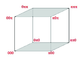
Figure 1: The eight Dirac points in the reciprocal space given by the corners of the cube. The grey faces are fix loci of the reflection $\mathcal{M}_{z}=i\Upsilon_{z}\Gamma_{7}.$

Second, the real space image of Fig 1 is given by the inverse Fourier transforms $\tilde{f}\left(x_{i},\Delta_{i}\right)$ of the functions $f\left(k_{i},\Delta_{i}\right)$; for the example of the x- component, we have

$$\tilde{f}_{x}=i\pi\left[\delta\left(x-a\right)-\delta\left(x+a\right)\right]$$ (36)

with peaks at $x=\pm a$ mod 2a where $a\equiv 1$ is the lattice parameter in x- direction. Similar relations can be also written down for the other directions; and a picture like the Figure 1 can be also drawn in real space.

III.3.2 Mirror symmetries

With the choice (35), the 3D hamiltonian thus obtained belongs to the BDI family of the AZ classification F1 ; F2 ; in addition to the CPT symmetries, the Hamiltonian (26) has also three reflections given by

$$\mathcal{M}_{x}H\left(k_{x},k_{y},k_{z};\mathbf{\Delta}\right)\mathcal{M}_{x}^{-1}$$

(37)

with the $\mathcal{M}_{i}$ mirrors realized as follows

$$\mathcal{M}_{x}=i\Upsilon_{x}\Gamma_{7}\text{\quad},\text{\quad}\mathcal{M}_{y}=i\Upsilon_{y}\Gamma_{7}\text{\quad},\text{\quad}\mathcal{M}_{z}=i\Upsilon_{z}\Gamma_{7}$$ (38)

The fix points of these $\mathcal{M}_{i}$’s are given by faces of the Figure 1; for example the fix points of $\mathcal{M}_{z}$ are given by the surfaces $\left(k_{x},k_{y},0\right)$ and $\left(k_{x},k_{y},\pi\right)$ represented by the grey surfaces of the Figure 1. Eqs(37) teach us that the hamiltonian has other symmetries induced by the composition of its basic symmetries namely $\mathcal{T}$, $\mathcal{C}_{i}$ and $\mathcal{M}_{i}$. For example, the composition of the $\mathcal{M}_{i}$’s amongst themselves like for inversion $\mathcal{I}$ reading as $i\mathcal{M}_{z}\mathcal{M}_{y}\mathcal{M}_{x}$ and realised by the generator $i\Lambda_{2}\Lambda_{4}\Lambda_{6}$. The common denominator of these operators and others is that they are symmetries of the gap energy (32). By substituting $k_{i\ast}=n_{i}\pi$ back into the expression of the gap energy, we get

$$E_{g}=2\sqrt{\left[\Delta_{x}-\cos n_{x}\pi\right]^{2}+\left[\Delta_{y}-\cos n_{y}\pi\right]^{2}+\left[\Delta_{z}-\cos n_{y}\pi\right]^{2}}$$ (39)

which vanishes for $\Delta_{i}=\left(-\right)^{n_{i}}$. At the Dirac point $k_{x\ast}=k_{y\ast}=k_{z\ast}=0$, the lines $\Delta_{x}=\Delta_{y}=\Delta_{z}=1$ in the moduli space $\mathcal{E}_{\Delta}$ define the frontier between the non trivial topological phase $\left|\Delta_{i}\right|<1$ and the trivial one given by $\left|\Delta_{i}\right|>1$.

IV Third order topological phase

In this section, we study the conditions for having higher order topological phases in the chiral model described above and give their solutions. First, we give the continuum limits of the lattice model (26) near the Dirac points and derive the HOT constraints. Then, we turn to construct the gapless corner states.

IV.1 Continuum limit and Dirac hamiltonian

Because of TRS symmetry, the 3D lattice model (35) has eight Dirac limits; the hamiltonians $H_{\mathbf{n}\pi}$ near these points are obtained by expanding (35) near $k_{i}=\kappa_{i\ast}+k_{i}^{\prime}$ (with $\kappa_{i\ast}=n_{i}\pi$), thus leading to the eight Dirac like hamiltonians living on the corners of the Figure 1

$$H_{\mathbf{n}\pi}=e^{in_{1}\pi}\Upsilon^{x}\left(k_{x}^{\prime}-i\phi_{x,n_{1}}\right)+e^{in_{2}\pi}\Upsilon^{y}\left(k_{y}^{\prime}-i\phi_{y,n_{2}}\right)+e^{in_{3}\pi}\Upsilon^{z}\left(k_{z}^{\prime}-i\phi_{z,n_{3}}\right)$$ (40)

In this parametric expression, $\mathbf{n}$ is a vector integer $\left(n_{1},n_{2},n_{3}\right)$ with $n_{i}=0,1$; and the $\phi_{l,n_{l}}$ are matrices given by $g_{l,n_{l}}\mathcal{C}_{l}$ with $\mathcal{C}_{l}$ as in (13) and the $g_{l,n_{l}}$’s are eight mass like parameters given by $g_{l,n_{l}}=1-e^{in_{l}\pi}\Delta_{l}$ and living at the faces of the Figure 1. For example $g_{x,0}=1-\Delta_{x}$ sits on the face $\left(0,k_{y},k_{z}\right)$ and $g_{x,\pi}=1+\Delta_{x}$ sits on $\left(\pi,k_{y},k_{z}\right)$.

IV.1.1 Mass parameters and gap energy

The eight Dirac hamiltonians (40) have the form $\Upsilon^{x}K_{x,\mathbf{n}\pi}+\Upsilon^{y}K_{y,\mathbf{n}\pi}+\Upsilon^{z}K_{z,\mathbf{n}\pi}$; they have quite similar structure; they differ only by the value of the $K_{l,\mathbf{n}\pi}$ coefficients in front of the gamma $\Upsilon_{l}$’s; so their studies are quite similar and we can restrict the analysis to one of them; say the Dirac limit near $\mathbf{k}_{\ast}=\left(0,0,0\right)$ namely

$$H_{\mathbf{0}}=\Upsilon^{x}\left(k_{x}-i\phi_{x}\right)+\Upsilon^{y}\left(k_{y}-i\phi_{y}\right)+\Upsilon^{z}\left(k_{z}-i\phi_{z}\right)$$ (41)

with

$$\phi_{x}=g_{1,0}\mathcal{C}_{x}\quad,\quad\phi_{y}=g_{2,0}\mathcal{C}_{y}\quad,\quad\phi_{z}=g_{3,0}\mathcal{C}_{z}$$ (42)

where $g_{l,0}=1-\Delta_{l}$; and where we have dropped out the prime in $k_{i}^{\prime}$. Here, we want to give three comments regarding the two above relations as they are at the basis in the study of HOT matter.

$\bullet$ Comment 1: three masses $m_{{}_{x}},m_{{}_{y}},m_{{}_{z}}$
If setting $k_{i}=0$ in (41), the eigenvalue equation $H_{\mathbf{0}}\Psi=E\Psi$ reduces to $-i\Upsilon^{l}\phi_{l}\Psi=E\Psi$; and by using (42), one can put it into the form $-i\Upsilon^{l}g_{l,0}\left(\mathcal{C}_{l}\Psi\right)=E\Psi$ with left hand side involving the quantities $\mathcal{C}_{l}\Psi$. By thinking of the wave function as an eigenstate of the fractional chiral charges, we can set $\mathcal{C}_{l}\Psi=\theta_{l}\Psi$, and then bring the energy eigenvalue equation to the form $-i\Upsilon^{l}m_{l}\Psi=E\Psi$ with $m_{l}$ given by

$$m_{x}=\theta_{{}_{x}}g_{x,0}\qquad,\qquad m_{y}=\theta_{{}_{y}}g_{y,0}\qquad,\qquad m_{z}=\theta_{z}g_{z,0}$$ (43)

and the $\theta_{{}_{x}},\theta_{{}_{y}},\theta_{{}_{z}}$ charges as in eq(14). These relations indicate that good mass- like parameters are given by $\left(m_{{}_{x}},m_{{}_{y}},m_{{}_{z}}\right)$ rather than $\left(g_{x,0},g_{y,0},g_{z,0}\right)$. The dependence of the mass terms in $\theta_{{}_{i}}$’s is a premise manifestation of the fractionalisation of the wave function.

$\bullet$ Comment 2: mass cube and partial chiral symmetries
The three $\theta_{i}$ charges of the partial chiral symmetry operators $\mathcal{C}_{i}$ take the values $\pm 1$; by substituting these values back into the triplet $\left(\theta_{{}_{x}},\theta_{{}_{y}},\theta_{{}_{z}}\right)$, one generates 8 possibilities related by $\mathcal{C}_{i}$ transformations; the first one is $\left(+,+,+\right),$ the second reads as $\left(-,-,-\right)$ and 6 more others ones; three of them have 2 $\left(+\right)$ and one $\left(-\right)$ like $\left(+,+,-\right)$, and the three others have 2 $\left(-\right)$ and one $\left(+\right)$ like $\left(-,-,+\right)$. These 8 possibilities can be also splitted into 4+4 sets: 4 triplets with a product $\theta_{{}_{x}}\theta_{{}_{y}}\theta_{{}_{z}}$ equals to +1; and 4 others with $\theta_{{}_{x}}\theta_{{}_{y}}\theta_{{}_{z}}=-1$,

$$\left(m_{x}^{+},m_{y}^{+},m_{z}^{+}\right)$$ , , ,

, , ,

(44)

This classification is helpful when computing Ind(H), the topological index of the hamiltonian. Notice that eq(44) is not sensitive to the signs of $g_{i,0}$; so we assume below $g_{i,0}>0$ and denote the positive $m_{i}$’s like $m_{i}^{+}=g_{i,0}$ and the negative ones as $m_{i}^{-}=-g_{i,0}$; they vanish at the fix points of $\mathcal{C}_{i}$. Notice also that (44) are precisely the corners A_i of the cube depicted by the Figure 2; these points belong to the moduli space $\mathcal{E}_{M}$ with coordinates $\left(\mu_{x},\mu_{y},\mu_{z}\right)$ with $\left|\mu_{i}\right|\leq g_{i,0}$.

Figure 2: The space $\mathcal{E}_{M}$ with variables $\left(\mu_{x},\mu_{y},\mu_{z}\right)$ describing mass cube $\left|\mu_{i}\right|\leq g_{i,0}$.

It is remarkable that despite the requirement $g_{i,0}>0,$ one do have positive masses but also negative ones; they are needed by higher order topology; in the limit $g_{z,0}\rightarrow 0$; the 3D cube given by the Figure 2 shrinks to the 2D olive-colored faces which merge; by taking also the limit $g_{y,0}\rightarrow 0$, the corresponding face shrinks to a 1D edge; and by performing moreover $g_{x,0}\rightarrow 0$, the line shrinks to the central point of the cube where live the AZ gapless state. From this view, the mass cube $\left|\mu_{i}\right|\leq g_{i,0}$ is just an irregular blow up of the $\mathcal{C}$ fix point leading to the fractionalisation of chiral symmetry as $\mathcal{C}_{x}\mathcal{C}_{y}\mathcal{C}_{z}$.

$\bullet$ Comment 3: gap energy
At $k_{i}=n_{i}\pi$,  the gap energy (45) can be expressed in two different, but equivalent, forms; either like $2(g_{x,0}^{2}+g_{y,0}^{2}+g_{z,0}^{2})^{1/2}$ as usually done; or more interestingly as follows

$$E_{g}=2\sqrt{m_{x}^{2}+m_{y}^{2}+m_{z}^{2}}$$ (45)

The two expressions are obviously equal since $m_{i}^{2}=\left(\theta_{i}g_{i,0}\right)^{2}$ is equal to $g_{i,0}^{2}$ due to the fact that $\theta_{i}=\pm 1$; the $E_{g}$ is not sensitive to the change of the sign of the mass parameters; i.e to the replacement $m_{i}\rightarrow-m_{i}$; so it is enough to study the situation at one corner of the Figure 2; say at $\left(m_{x}^{+},m_{y}^{+},m_{z}^{+}\right)$ and use the above $\mathcal{C}_{i}$ symmetries to deduce the picture at the other corners. Recall that for AZ matter, the topological transition takes place at the fix point of $m_{i}\rightarrow-m_{i}$ corresponding to the vanishing of masses; this is the fix point of the chiral symmetry $\Gamma_{7}$ thought of as $\mathcal{C}_{{}_{x}}\mathcal{C}_{{}_{y}}\mathcal{C}_{z}$.

IV.1.2 Higher order topological matter

We begin by recalling that 3D topological AZ matter has: $\left(1\right)$ two periodic boundaries and one open direction (say x- and y- periodic but z- open). $\left(2\right)$ gapped states in the 3D bulk but gapless surface states on the boundary. Regarding the 3D HOT we are studying here, all the three real directions of the 3D material are open and has gapless corners states; see Appendix A. To build the gapless corner states, we start from eqs(41-42), and proceed in two steps as follows:
First, we demand the bulk states of HOT matter to be gapped; that is $E_{g}>0$; this is a necessary condition for higher order topological matter. A direct implication of this constraint follows from eq(45); it indicates that at least one of the three $m_{l}$ masses must be non vanishing in order to have a non zero bulk gap. In terms of the $\Delta_{l}$ coupling constants, at least one of the three  should be different from $1$. For a third order topological phase, the condition of non vanishing gap is fulfilled by the non vanishing of the three masses; i.e $m_{l}\neq 0$; these three conditions can be stated as follows

$$m_{x}m_{y}m_{z}\neq 0$$ (46)

Second, we map (41) to the real space with coordinates $\mathbf{r}=\left(x,y,z\right)$ in order to exhibit explicitly the effect of demanding the constraint (46); with this mapping the delta Dirac distribution $\delta_{3}\left(\mathbf{k}-\mathbf{k}_{\ast}\right)$ turns into a 3D space integral of the plane wave $e^{-i\left(\mathbf{k}-\mathbf{k}_{\ast}\right).\mathbf{r}}$ and the vector $\mathbf{k}$ is represented by the operator $\partial/i\partial\mathbf{r}$; then the hamiltonian involved in the energy eigenvalue equation $H_{\mathbf{0}}\hat{\Psi}\left(\mathbf{r}\right)=E\hat{\Psi}\left(\mathbf{r}\right)$ reads as

$$H_{\mathbf{0}}=\Upsilon^{x}\left(\frac{\partial}{i\partial x}-i\phi_{x}\right)+\Upsilon^{y}\left(\frac{\partial}{i\partial y}-i\phi_{y}\right)+\Upsilon^{z}\left(\frac{\partial}{i\partial z}-i\phi_{z}\right)$$ (47)

Notice that besides its differential nature, $H_{\mathbf{0}}$ is still an 8$\times$8 matrix operator and $\hat{\Psi}\left(\mathbf{r}\right)$ is a complex spinor with eight components. Notice also that the $\phi_{i}$’s are matrix masses that have to be treated carefully when looking for solution of the eigenstates of $H_{\mathbf{0}}$. To engineer gapless states while preserving the constraint (46), we look for exotic (non oscillating) wave functions $\Psi\left(\mathbf{r}\right)$ solving the equation $H_{\mathbf{0}}\Psi\left(\mathbf{r}\right)=0$. Clearly a solution of such zero mode equation exists and has the form of an evanescent wave

$$\Psi\left(\mathbf{r}\right)=\mathcal{N}e^{-\mathbf{m}.\left(\mathbf{r-r}_{0}\right)}\Omega$$ (48)

with vector $\mathbf{m}$ referring to $\left(m_{x},m_{y},m_{z}\right)$ and where $\mathbf{r}_{0}$ is some given space position; it is imagined as a corner. The use of $\mathbf{m}$ instead of the $\phi_{i}$’s is because of their relationship (43) and also because of (44).

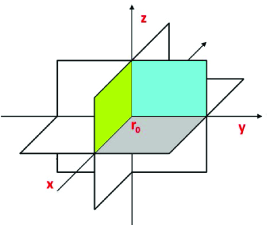
Figure 3: An octant of the 3D space $\mathbb{R}^{3}$ with corner at $\mathbf{r}_{0}$; it is given by $\frac{1}{8}$ of $\mathbb{R}^{3}$. Octants of $\mathbb{R}^{3}$ are defined by the signs of $x-x_{0},$ $y-y_{0}$ and $z-z_{0}.$

The factor $\mathcal{N}$ is a normalisation constant and the factor $\Omega$ is a constant spinor with eight component; it gives the polarisation of $\Psi\left(\mathbf{r}\right)$. Notice also that the existence of the candidate solution (48) can be also motivated from the gap energy formula $E_{g}=2\sqrt{m_{j}^{2}+k_{j}^{2}}$ which never vanishes as far as (46) holds and as long as the $k_{j}$’s are real numbers. However, a vanishing $E_{g}$ is possible for pure imaginary momenta $k_{j}=im_{j}$ indicating that gapless states are given by corner waves.

IV.2 Gapless corner states

Here, we sit in a particular region in the moduli space $\mathcal{E}_{M}$ with coordinates $\left(\mu_{x},\mu_{y},\mu_{z}\right)$; in addition to the constraint (46), we assume moreover

$$m_{x}>0\quad,\quad m_{y}>0\quad,\quad m_{z}>0$$ (49)

This choice corresponds to sitting at the $\left(m_{x}^{+},m_{y}^{+},m_{z}^{+}\right)$ point of the set (44); it is one of eight possibilities corresponding to the eight corners of the Figure 2; the above (49) corresponds to the corner A7. To that purpose, we first derive the solution (48) describing gapless corner states; then we turn to give some of their characteristic properties.

IV.2.1 Deriving Eq(48)

We begin by expressing the gapless state equation $H_{\mathbf{k}}\Psi=0$ as

$$\left(-i\mathbf{\Upsilon}^{x}\mathcal{D}_{x}-i\mathbf{\Upsilon}^{y}\mathcal{D}_{y}-i\mathbf{\Upsilon}^{z}\mathcal{D}_{z}\right)\Psi=0$$ (50)

with

$$\mathcal{D}_{i}=\partial_{i}-\phi_{i}$$ (51)

and $\phi_{i}$ mass matrices as

$$\phi_{x}=g_{x}\mathcal{C}_{x}\quad,\quad\phi_{y}=g_{y}\mathcal{C}_{y}\quad,\quad\phi_{z}=g_{z}\mathcal{C}_{z}$$ (52)

where the $\mathcal{C}_{i}$’s are given by (13). Since these $\mathcal{C}_{i}$’s are hermitian matrices and they commute; i.e: $\mathcal{C}_{i}\mathcal{C}_{j}=\mathcal{C}_{j}\mathcal{C}_{i}$; it results that the $\phi_{i}$’s are hermitian as well and they commute between them. So, the solution of (50) can be factorised as

$$\Psi\left(x,y,z\right)=\mathcal{N}e^{-\phi_{x}\left(x-x_{0}\right)}e^{-\phi_{y}\left(y-y_{0}\right)}e^{-\phi_{z}\left(z-z_{0}\right)}\Omega$$ (53)

with $\Omega$ a constant unit spinor with components $\left(\omega_{1},...,\omega_{8}\right)$. By constant spinor $\Omega$, we mean that it is space coordinate independent like $\partial\Omega/\partial x=0$ and so on; and by unit spinor we refer to the normalisation $\left|\omega_{1}\right|^{2}+...+\left|\omega_{8}\right|^{2}=1.$ These two specific features can be stated as follows:

$$\partial_{i}\Omega=0\quad,\quad tr\left(\Omega^{+}\Omega\right)=1$$ (54)

Using these properties, we can compute the normalisation factor $\mathcal{N}$ by using the relation $\int_{\mathbb{R}^{3}}tr\left(\Psi^{+}\Psi\right)d^{3}\mathbf{r}=1$. But to perform this calculation, we need to know the value of $tr\left(\Psi^{+}\Psi\right)$ which requires the introduction of the charge vector $\boldsymbol{q}$ with components $(q_{{}_{x}},q_{{}_{y}},q_{{}_{z}})$; this need of $\boldsymbol{q}$ is because of the matrix masses $\phi_{i}=g_{i}\mathcal{C}_{i}$ appearing in the exponentials of eq(53). So, normalisable solutions depend on the values of the charge vector $\boldsymbol{q}$ as shown below

$$\Psi_{\boldsymbol{q}}=\mathcal{N}e^{-m_{x}\left(x-x_{0}\right)}e^{-m_{y}\left(y-y_{0}\right)}e^{-m_{z}\left(z-z_{0}\right)}\Omega_{\boldsymbol{q}}$$ (55)

where we have used (43) and the eigenstate equation $\mathcal{C}_{i}\Omega_{\boldsymbol{q}}=\theta_{i}\Omega_{\boldsymbol{q}}$ whose solution were studied in subsection 2.2. Depending on the sign of $(m_{{}_{x}},m_{{}_{y}},m_{{}_{z}})$, the normalisation of $\Psi_{\boldsymbol{q}}$ requires $x-x_{0}$, $y-y_{0}$ and $z-z_{0}$ having respectively the same sign as the sign of $m_{{}_{x}},m_{{}_{y}},m_{{}_{z}}$. In this case, we have

$$\mathcal{N}=\frac{1}{\sqrt{8\left|m_{x}m_{y}m_{z}\right|}}$$ (56)

Notice that in the case where $sgn\left(m_{i}\right)$ are positive, we must have

$$x>x_{0}\qquad,\qquad y>y_{0}\qquad,\qquad z>z_{0}$$ (57)

These three inequalities define an octant of the 3D space $\mathbb{R}^{3}$, the three line sides intersect at the point $\left(x_{0},y_{0},z_{0}\right)$ giving the corner of the octant. The relationship between the signs of $(m_{x},m_{y},m_{z})$ and the corners of the Figure 2 is given by the following table

$${\small m_{x},m_{y},m_{z}}$$

Fig 2 A1 A2 A3 A4 A5 A6 A7 A8

IV.2.2 Chiral wave functions

A gapless chiral wave function $\Psi$ obeys the zero mode equation $H\Psi=0$ and moreover carries a definite charge $q_{{}_{\Gamma_{7}}}$ under the chiral operator $\Gamma_{7}.$ Since $q_{{}_{\Gamma_{7}}}$ can take the values $\pm 1,$ we distinguish two types of chiral wave spinors: right handed $\Psi_{R}$ with $q_{{}_{\Gamma_{7}}}=+1$ and a left handed $\Psi_{L}$ with $q_{{}_{\Gamma_{7}}}=-1$. In other words, gapless right and left handed wave functions are defined as

$$H\Psi_{R}=0$$

(58)

The solutions of the chirality conditions are given by eqs(21) and (22) showing that they are combinations of four terms. Below, we show that the eight possible polarisations of the $\Psi_{R}/\Psi_{L}$ states will be dispatched on the corners of the mass cube according to the valuesof the charges $\theta_{i}$ of the observables $\mathcal{C}_{i}$. For that, notice that the polarisation of the gapless wave function $\Psi$ (53) is carried by the constant spinor $\Omega$; and because of (52), it results that gapless right handed and left handed states are given by

$$\Psi_{\mathbf{q,}R}$$

(59)

with vector $\mathbf{q}$ referring to $(q_{{}_{x}},q_{{}_{y}},q_{{}_{z}})$ and polarisations $\Omega_{\mathbf{q,}R}$ and $\Omega_{\mathbf{q,}L}$ as follows

$$\Gamma_{7}\Omega_{\mathbf{q,}R}=\Omega_{\mathbf{q,}R}\qquad,\qquad\Gamma_{7}\Omega_{\mathbf{q,}L}=-\Omega_{\mathbf{q,}L}$$ (60)

The chiral wave functions $\Psi_{R}$ and $\Psi_{L}$ have been fractionalized into $\Psi_{\mathbf{q,}R}$ and $\Psi_{\mathbf{q,}L}$. Notice also that in the limit $m_{i}\rightarrow 0,$ the fractional waves $\Psi_{\mathbf{q,}R/R}$ tend to $\Omega_{\mathbf{q,}R}\mathbf{\delta}_{3}\left(\mathbf{r}-\mathbf{r}_{0}\right)$ where $\mathbf{\delta}_{3}$ is the usual 3D Dirac delta function. Below, we determine these gapless chiral waves and give their properties.

V Right and left handed states

In this section, we give specific properties of fractional chiral states. First, we focus on the study of gapless states with fractional right and left handed chiralities. Then, we use these fractional chiral states to calculate the topological index of the eight band model.

V.1 Chiral polarisations $\Omega_{\mathbf{q,}R}$ and $\Omega_{\mathbf{q,}L}$

From eqs(59), we learn that the fractional chiral wave functions $\Psi_{\mathbf{q,}R}$ and $\Psi_{\mathbf{q,}L}$ are given by the product of two factors: the extrinsic factor $\mathcal{N}e^{-\mathbf{m}\left(\mathbf{r}-\mathbf{r}_{0}\right)}$ shared by both waves; and intrinsic factors given by $\Omega_{\mathbf{q,}R}$ and $\Omega_{\mathbf{q,}L}$ carrying their polarisations. The explicit expressions of these polarisations are derived below.

V.1.1 Right handed polarisation

To study the properties of the gapless right handed chirality of $\Omega_{\mathbf{q,}R}$, we have to look for the allowed possibilities of the constant spinors $\Omega_{\mathbf{q,}R}$ solving (60). For that, we use the factorized representation (8) to express the wave function polarisation $\Omega_{\mathbf{q}}$ as follows

$$\Omega_{\mathbf{q}}=\mathbf{a}_{q_{{}_{\varrho_{{\small 3}}}}}\mathbf{b}_{q_{{}_{\tau_{{\small 3}}}}}\mathbf{c}_{q_{{}_{\sigma_{{\small 3}}}}}$$ (61)

where $\mathbf{a}_{\pm},\mathbf{b}_{\pm}$ and $\mathbf{c}_{\pm}$ are two- component constant spinors.normalised as

$$\mathbf{e}_{+}=\left(\begin{array}[]{c}1\\ 0\end{array}\right)\qquad,\qquad\mathbf{e}_{-}=\left(\begin{array}[]{c}0\\ 1\end{array}\right)$$ (62)

with $\mathbf{e}_{\pm}$ standing for $\mathbf{a}_{\pm},\mathbf{b}_{\pm}$ and $\mathbf{c}_{\pm}$. Recall that the $\theta$ vector charge $(\theta_{{}_{x}},\theta_{{}_{y}},\theta_{{}_{z}})$ is related to the $\mathbf{q}$ charge vector as $(-q_{{}_{\sigma_{{\small 3}}}},q_{{}_{\tau_{{\small 3}}}}q_{{}_{\sigma_{{\small 3}}}},q_{{}_{\varrho_{{\small 3}}}})$. By help of (8), the chirality of $\Omega_{\mathbf{q}\text{,}R}$ can be deduced from the value of $q_{{}_{\mathbf{\Gamma}_{7}}}=-q_{{}_{\varrho_{3}}}q_{{}_{\tau_{3}}}$ which indicates that right handed wave function must have $q_{{}_{\varrho_{3}}}q_{{}_{\tau_{3}}}=-1$; but $q_{{}_{\sigma_{{\small 3}}}}$ free that is taking both values $\pm 1$. As the condition $q_{{}_{\varrho_{3}}}q_{{}_{\tau_{3}}}=-1$ has two solutions namely $\left(q_{{}_{\varrho_{3}}},q_{{}_{\tau_{3}}}\right)$ equals either to $\left(1,-1\right)$ or to $\left(-1,1\right)$; it follows that there are four solutions classified by the Pauli charge vectors

$$\mathbf{q}=\left(1,-1,\pm 1\right)\qquad,\qquad\left(-1,1,\pm 1\right)$$ (63)

Therefore, we have the four following $\Omega_{\mathbf{q},R}$ configurations

$$\left(q_{{}_{\varrho_{3}}},q_{{}_{\tau_{3}}},q_{{}_{\sigma_{{\small 3}}}}\right)$$

(64)

However, not all these $\Omega_{\mathbf{q},R}$ configurations can be substituted into (59); this is because of the correlation between that the mass vector $\mathbf{m}$ and the position vector $\left(\mathbf{r-r}_{0}\right)$ as the convergence of tr$\left(\Psi_{\mathbf{q,}R}^{+}\Psi_{\mathbf{q,}R}\right)$ requires

$$\theta_{x}\left(x-x_{0}\right)>0\qquad,\qquad\theta_{y}\left(y-y_{0}\right)>0\qquad,\qquad\theta_{z}\left(z-z_{0}\right)>0$$ (65)

Recall that tr$\left(\Psi_{\mathbf{q,}R}^{+}\Psi_{\mathbf{q,}R}\right)$ is equal to $\mathcal{N}e^{-2m_{x}\left(x-x_{0}\right)}e^{-2m_{y}\left(y-y_{0}\right)}e^{-2m_{z}\left(z-z_{0}\right)}$ times tr$\left(\Omega_{\mathbf{q,}R}^{+}\Omega_{\mathbf{q,}R}\right)=1$. In these exponentials, the masses are given by $m_{i}=\theta_{i}g_{i,0}$ as one sees on eq(49), and because of our assumption $g_{i,0}>0,$ it results that convergence of tr$\left(\Psi_{\mathbf{q,}R}^{+}\Psi_{\mathbf{q,}R}\right)$ requires $\theta_{x}$ and $\left(x-x_{0}\right)$ to have the same sign so that $e^{-2m_{x}\left(x-x_{0}\right)}$ vanishes when $m_{x}\left(x-x_{0}\right)\rightarrow+\infty$. For the same reason, it requires also that $\theta_{y}$ and $\left(y-y_{0}\right)$ should have the same sign and similarly for $\theta_{z}$ and $\left(z-z_{0}\right)$. As such, according to the signs of $(\theta_{{}_{x}},\theta_{{}_{y}},\theta_{{}_{z}}),$ normalised gapless states $\Psi_{\mathbf{q,}R}$ are given by

Fig 2 $$sgn({\small m}_{{}_{x}}{\small,m}_{{}_{y}}{\small,m}_{{}_{z}})$$

A1          

A3          

A5          

A7          

(66)

where ${\small\tilde{x}}=x-x_{0}$ and so on. Gapless right handed states occupy four of the eight corners of the Figure 2; so one expects that the other four corners are occupied by gapless left handed states; this feature is shown below.

V.1.2 Left handed polarisation

Gapless left handed wave function $\Psi_{L}$ can be obtained by repeating the above steps of calculations. The constraint $\Gamma_{7}\Omega_{L}=-\Omega_{L}$ requires $q_{{}_{\mathbf{\Gamma}_{7}}}=-1$ and leads to the four following $\Omega_{\mathbf{q},L}$ configurations

$${\small(q}_{{}_{\varrho_{{\small 3}}}}{\small,q}_{{}_{\tau_{{\small 3}}}}{\small,q_{{}_{\sigma_{3}}})}$$

(67)

The locations of these gapless left handed states in the mass space $\mathcal{E}_{M}$ are collected in the following table

Fig 2 sgn$${\small(m}_{{\small x}}{\small,m}_{{}_{y}}{\small,m}_{{}_{z}}{\small)}$$

A2        

A4      

A6      

A8          

(68)

they occupy precisely the remaining corners in table (66).

V.2 Computing the topological index

In this subsection, we calculate the topological index (IndH) of the chiral hamiltonian H_k of the eight bands lattice model. This is an integer number given by the difference $n_{R}-n_{L}$ counting the number of chiral gapless states of the higher order topological model. To determine IndH, we apply the index theorem on open spaces G1 ; G2 ; G3 ; G4 ; G5 to the hamiltonian (26) and use a practical formula obtained recently in nous . To that purpose, we start from (26) with coefficients $f_{i}=f\left(k_{i}\right)$ and $g_{i}=g\left(k_{i},\Delta_{i}\right)$ as in (35) and gap energy relation as in (45); the continuum limit of (26) leads to eight Dirac- like hamiltonians H_nπ sitting at the eight corners of BZ represented by the Figure 1. At each one of these corners, the gap energy $E_{g}$ has the same expression which is given by $2(k_{i}^{2}+m_{i}^{2})^{1/2}$; thanks to mirror $\mathcal{M}_{l}$ and the fractional chiral symmetries $\mathcal{C}_{l}$. So, gapless states are of two kinds: First massless states with $k_{i}=0$, but this is not our case. Second, massive states sitting at the eight corners of the cube of the Figure 2; these gapless states are described by evanescent waves with fractional chiral polarisation; they are given by wave function type $\left|m_{x}m_{y}m_{z}\right|^{-1/2}e^{-\mathbf{m.\tilde{r}}}\Omega_{\mathbf{q}}$ with definite polarisation $\Omega_{\mathbf{q}}$ characterising the HOT matter. By combining the two Figures 1 and 2, one gets a total number of 64 massive corner states in the chiral lattice model (26). Consequently, IndH is equal to 64 times the contribution of a corner state to the topological index which turns out to be given by the unit $\mathop{\displaystyle\prod}\nolimits_{i}\frac{1}{2}\left[sgn(m_{i}^{+})-sgn(m_{i}^{-})\right]$. This result can be also derived by first expressing IndH as the sum $\sum_{\mathbf{n}}$Ind(H_nπ) with integer vector $\mathbf{n}=\left(n_{x},n_{y},n_{z}\right)$ and $n_{i}=0,1$. Then, using the property that the eight Dirac- like hamiltonians $H_{\mathbf{n\pi}}$ have same ground state properties as $H_{\mathbf{0\pi}}$; this leads to IndH equals to 8 times Ind(H_0π). To calculate the explicit value of Ind(H_0π), we use the formula of nous according to which the topological index for cube like geometries is given by sgn functions as follows

Ind(H_0π) $$=$$

(69)

To apply this formula to our situation, we think of the eight triplets $\left(a_{\pm},b_{\pm},c_{\pm}\right)$ appearing in above relations as just the mass triplets $\left(m_{x}^{\pm},m_{y}^{\pm},m_{z}^{\pm}\right)$ defining the coordinates of the eight corner points A₁,…,A₈ of the Figure 2. For the case of corners A1- A3- A5- A7, the associated sgn functions are learnt from the table (66), thus leading to

Fig 2 $$({\small m}_{{}_{x}}{\small,m}_{{}_{y}}{\small,m}_{{}_{z}})$$ Ind(H_0π)

A1        

A3        

A5        

A7        

(70)

Similarly, the sgn functions associated A2- A4- A6- A8 are read from the table (68) leading to,

Fig 2 $${\small sgn(m}_{{\small x}}{\small,m}_{{}_{y}}{\small,m}_{{}_{z}}{\small)}$$ Ind(H_0π)

A2        

A4        

A6        

A8        

(71)

So the total value of Ind(H_0π) is equal to 1 and the total contribution for the chiral lattice model is 8; which is equal to the number of Dirac points; it is also equal 64 times the index contribution of a fractional right (left) handed state.

VI Conclusion and discussions

In this paper, we have studied the anomalous properties of a family of massive fermion models describing higher order topological matter. We have considered chiral eight models and showed that they have 26 degrees of freedom; six of them are basic ones and give the essence on the higher order topological properties of these matter systems. We have computed the explicit expressions of the gapless states for third order topological category and showed that they are given by chiral fractional states occupying the corners of the Figure 2. These fractional states carry, in addition to the charge $q_{{}_{\Gamma_{7}}}$ of $\mathcal{C}$, three other charges $q_{{}_{x}},q_{y},q_{{}_{z}}$ whose product is equal to $q_{{}_{\Gamma_{7}}}$. This charge fractionalization aspect gives a bridge between conventional chiral AZ matter and 3D chiral higher order topological phases. We have also calculated the contribution of these gapless states to the topological index; we found that the total value of IndH is 8; it is obtained by summing over all possible contributions which is given by 64 times the contribution of each corner to the index.

VII Appendix

In this appendix, which is organised in four parts (A, B, C, D), we give some useful details regarding the topological chiral model studied in this paper. First, we describe some known results on 3D HOT matter with focus on the corner states (Appendix-A). Then, we show how the eight band model we have studied in this work is a minimal model (Appendix-B). We take this occasion to draw the main line to build non minimal models in 3D. After that, we describe how to engineer the matter couplings in the real lattice (Appendix-C). We end this appendix by giving a comment on what we called fractional (1/3 and 2/3) symmetries in the main text (Appendix-D).

Appendix $\mathbf{A}.$ 3D HOT matter and corner states
We begin by recalling that some facts about 3D topological AZ matter and 3D HOT matter. Three dimensional topological matter of the AZ table has some unified aspects; in particular: $\left(1\right)$ A real 3D lattice with two periodic boundaries and one open direction. For the example of cubic matter, one can imagine the periodic boundaries as given by the x- and y- directions and the open one by the z- dimension. $\left(2\right)$ Gapped states in the 3D bulk but gapless states on the boundary surface. In other words, 3D topological AZ matter is characterised by gapped bulk states and gapless surface states.
Regarding the 3D HOT we studied in this paper, the D/D-1 correspondence is relaxed to D/D-3. Seen that here D=3, the topological boundary states are then given by 0D states or corners states. This picture corresponds to the situation where all the three real (x,y,z) directions of the 3D material are open. In this case, the boundary surface surrounding the cubic volume is a non- regular surface in the sense it is made of: $\left(i\right)$ 6 types of 2D faces F namely: the upper face F${}_{xy}^{+}$ and the bottom face F${}_{xy}^{-}$; the front F${}_{yz}^{+}$ and the behind F${}_{yz}^{-}$; left F${}_{zx}^{+}$ and the right F${}_{zx}^{-}$. $\left(ii\right)$ 12 line edges given by: 4 segments in x-direction, 4 segments in y-direction and 4 segments in z-direction. $\left(iii\right)$ 8 corners given by the intersections of line edges (or also by intersections of three normal faces). These 8 corners are particularly interesting for us as they host the gapless states of HOT matter we are studying in this paper. Being gapless, these corner states obey massless Dirac-like equation $D\psi_{corner}=0$ where $D$ the Dirac-like operator which in our study is given by eqs(47) and (50). The solutions of this equation is studied in the main text.

Appendix $\mathbf{B}.$ Chiral multi-bands
The chiral eight band model which we have studied in this paper is a minimal 3D model that extends the well known SSH model with open boundary. It describes gapless corner states of 3D HOT matter. To see the minimality feature, it is interesting to recall a known result on Dirac-like matter in diverse space dimensions. Because of the Gamma matrices of the Dirac-like Hamiltonian, the number N of bands is quantized like $n\times 2^{d}$ where $2^{d}$ is the number of components of each Dirac-like field $\mathbf{\psi}$ and n referring to the number of matter fields (the number of spinors). This relation means that for $d=1,$ corresponding to SSH, the number N=2n with n for conduction band and n for valence band. For the d=2 and the d=3 extensions of SSH, the number of bands is respectively given by $n\times 2^{2}=4n$ and $n\times 2^{3}=8n$. So, the eight band 3D model studied in present paper is a minimal model (n=1). However, the generalisation of our modeling to chiral 8n bands goes straightforwardly. The basic idea in the construction consists in replacing one of the 2$\times$2 Pauli matrices by the following generalised $2n\times 2n$ matrices. For example, by replacing $\rho_{x},$ $\rho_{y},$ $\rho_{z}$ by the following $2n\times 2n$ matrices $R_{x},$ $R_{y},$ $R_{z}$.

$$R_{x}=\left(\begin{array}[]{cc}0&I_{n}\\ I_{n}&0\end{array}\right)\quad,\quad R_{y}=\left(\begin{array}[]{cc}0&-iI_{n}\\ iI_{n}&0\end{array}\right)\quad,\quad R_{z}=\left(\begin{array}[]{cc}I_{n}&0\\ 0&-I_{n}\end{array}\right)$$ (B1)

where $I_{n}$ is the $n\times n$ identity matrix.

Appendix $\mathbf{C}$. Couplings in real lattice
The eight band Hamiltonian (35) is expressed in the reciprocal space. This hamiltonian can be also expressed in the real space. The derivation of the real interactions leading to (35) is commented below. First, we consider the Dirac-like matter field $\mathbf{\psi}\left(\mathbf{r}_{i}\right)\equiv\mathbf{\psi}_{\mathbf{r}_{i}}$ at site positions $\mathbf{r}_{i}$ (for short $\mathbf{r}$) of the real 3D cubic lattice. This matter field has eight components $\left(\psi_{1\mathbf{r}},...,\psi_{8\mathbf{r}}\right).$ Then, we denote the nearest neighbours to $\mathbf{r}$ by $\mathbf{r+a}_{j}$ with the three cubic vectors as usual; that is $\mathbf{a}_{x}=ae_{x},$ $\mathbf{a}_{y}=ae_{y},$ $\mathbf{a}_{z}=ae_{z}.$ After that, we use the $\Upsilon^{j}$ and $\Lambda^{j}$ matrices of eq(7) to couple the nearest neighbours $\mathbf{\psi}_{\mathbf{r}}$ and $\mathbf{\psi}_{\mathbf{r+a}_{j}}$ as follows

$$\mathbf{\psi}_{\mathbf{r}}^{\dagger}\Upsilon^{i}\mathbf{\psi}_{\mathbf{r+a}_{j}}$$ , ; ,

(C.1)

In these couplings, the $\Upsilon^{x}$ and $\Lambda^{x}$ are linked with the direction $\mathbf{a}_{x}$; the same thing is done for the other matrices. Next, we engineer: $\left(1\right)$ the terms in $\sin k_{j}$ by using pseudo-real couplings like

$$h_{1}=-i\sum\limits_{\mathbf{r},\mathbf{a}_{j}}t_{j}\left[\mathbf{\psi}_{\mathbf{r}}^{\dagger}\Upsilon^{i}\mathbf{\psi}_{\mathbf{r+a}_{j}}-\mathbf{\psi}_{\mathbf{r+a}_{j}}^{\dagger}\Upsilon^{j}\mathbf{\psi}_{\mathbf{r}}\right]$$ (72)

and $\left(2\right)$ the terms in $\cos k_{j}$ by using real coupling as follows $h_{2}=\sum t_{j}^{\prime}(\mathbf{\psi}_{\mathbf{r}}^{\dagger}\Lambda^{j}\mathbf{\psi}_{\mathbf{r+a}_{j}}+\mathbf{\psi}_{\mathbf{r+a}_{j}}^{\dagger}\Lambda^{j}\mathbf{\psi}_{\mathbf{r}}).$ The terms in $\Delta_{j}$ are given by $h_{3}=\sum\Delta_{j}\mathbf{\psi}_{\mathbf{r+a}_{j}}^{\dagger}\Lambda^{j}\mathbf{\psi}_{\mathbf{r+a}_{j}}.$

Appendix $\mathbf{D}.$ ”Fractional” symmetries
Here we give a group theoretical description of the chiral symmetry $\Gamma_{7}=\mathcal{C}=\mathcal{C}_{x}\mathcal{C}_{y}\mathcal{C}_{z}$ acting on the hamiltonian as in eq(1) and on the functions $f_{x}$ and $g_{x}$ like in (30). The action of the chiral operator $\mathcal{C}_{x}\mathcal{C}_{y}\mathcal{C}_{z}$ on the six components $f_{x},g_{x};f_{y},g_{y};f_{z},g_{z}$ appearing in the Hamiltonian (26) reads as follows

$$\mathcal{C}_{x}$$ :

:

:

(D.1)

By using group theory language, each transformation $\mathcal{C}_{i}$ generates a symmetry group $\mathbb{Z}_{2}$ with elements as $\left\{I_{id},-I_{id}\right\}$. So, the combination of the three transformations (A1) generate the discrete group product $\mathbb{Z}_{2}\times\mathbb{Z}_{2}\times\mathbb{Z}_{2}$. For convenience, we denote this symmetry group like $\mathbb{Z}_{2}^{x}\times\mathbb{Z}_{2}^{y}\times\mathbb{Z}_{2}^{z}$ where we have exhibited the x- , y- and z- directions. The first $\mathbb{Z}_{2}^{x}$ is generated by $\mathcal{C}_{x}$, the second by $\mathcal{C}_{y}$ and the third by $\mathcal{C}_{z}$. Seen that $\mathbb{Z}_{2}\times\mathbb{Z}_{2}\times\mathbb{Z}_{2}$ is the full chiral symmetry, the sub-symmetry $\mathbb{Z}_{2}^{x}$ generated by $\mathcal{C}_{x}$ is then a particular sub-symmetry (1/3 symmetry for short). Similarly, the sub-summetry $\mathbb{Z}_{2}^{x}\times\mathbb{Z}_{2}^{y}$ generated by the composition $\mathcal{C}_{x}\mathcal{C}_{y}$ is 2/3 chiral symmetry of the full $\mathcal{C}$. Notice that similar things can be also said about the other 1/3 symmetries namely $\mathbb{Z}_{2}^{y}$ and $\mathbb{Z}_{2}^{z}$ as well as about the 2/3 symmetries $\mathbb{Z}_{2}^{x}\times\mathbb{Z}_{2}^{z}$ and $\mathbb{Z}_{2}^{y}\times\mathbb{Z}_{2}^{z}$.

   

Acknowledgment 1

Professors Lalla Btissam Drissi and El Hassan Saidi would like to acknowledge ”Académie Hassan II des Sciences et Techniques-Morocco” for financial support. They thank also Felix von Oppen for stimulating discussions. L. B. Drissi acknowledges the Alexander von Humboldt Foundation for financial support via the Georg Forster Research Fellowship for experienced scientists (Ref 3.4 - MAR - 1202992).

References

• (1) Edward Witten, Fermion Path Integrals And Topological Phases, Rev. Mod. Phys. 88, 35001 (2016), arXiv:1508.04715.
• (2) Edward Witten, Three Lectures On Topological Phases Of Matter, La Rivista del Nuovo Cimento, 39 (2016) 313-370.
• (3) Ching-Kai Chiu, Jeffrey C. Y. Teo, Andreas P. Schnyder, and Shinsei Ryu, Classification of topological quantum matter with symmetries - Rev. Mod. Phys. 88, 035005 (2016)
• (4) Shinsei Ryu et al, Topological insulators and superconductors: tenfold way and dimensional hierarchy 2010 New J. Phys. 12 065010.
• (5) C. G. Callan, Jr., and J. A. Harvey, “Anomalies and fermion zero-modes on Strings and domain walls,” Nucl.Phys. B250 (1985) 427.
• (6) X. Chen, Z.-C. Gu, Z.-X. Liu, and X.-G. Wen, “Symmetry protected topological orders and the group cohomology of their symmetry group,” Phys. Rev. B87 (2013) 155114.
• (7) D. S. Freed, “Anomalies and invertible field theories,” arXiv:1404.7224.
• (8) E.H Saidi, Gapped gravitinos, isospin $1/2$ particles and $N=2$ partial breaking, Prog Theor Exp Phys (2019), arXiv:1812.04509.
• (9) A. Borici, Creutz fermions on an orthogonal lattice, Phys. Rev. D 78 (2008) 074504.
• (10) P.F. Bedaque, M.I. Buchoff, B.C. Tiburzi and A. Walker-Loud, Search for Fermion Actions on Hyperdiamond Lattices, Phys. Rev. D 78 (2008) 017502.
• (11) M. Creutz, T. Kimura and T. Misumi, Aoki Phases in the Lattice Gross-Neveu Model with Flavored Mass terms, Phys. Rev. D 83 (2011) 094506.
• (12) L. B. Drissi, H. Mhamdi, E.H. Saidi, Anomalous Quantum Hall Effect of 4D Graphene in Background Fields, Journal High Energy Physics JHEP 10 (2011) 026.
• (13) L. B. Drissi, E. H. Saidi, A signature index for third order topological insulators, J. Phys: Cond. Matt, 32 (36) (2020) 365704.
• (14) B. Ozyilmaz, et al., Phys. Rev. Lett. 99 (2007) 166804.
• (15) R. Jackiw, A.I. Milstein, S.-Y. Pi, I.S. Terekhov, Phys. Rev. B 80 (2009) 033413.
• (16) L. B. Drissi, E.H. Saidi, Dirac Zero Modes in Hyperdiamond Model, Phys. Rev. D 84, 014509, (2011).
• (17) Jia-An Yan, Lede Xian, M.Y. Chou, Phys. Rev. Lett. 103 (2009) 086802.
• (18) K.S. Novoselov, et al., Nature 438 (2005) 197–200.
• (19) L. B. Drissi, E.H. Saidi, M. Bousmina, Electronic properties and hidden symmetries of graphene, Nucl.Phys.B, Volume 829, Issue 3, (2010).
• (20) T. Kimura and T. Misumi, Lattice fermions based on higher-dimensional hyperdiamond lattices, Prog. Theor. Phys. 123 (2010) 63–78 523–533.56.
• (21) L.B. Drissi, E.H. Saidi and M. Bousmina, Four Dimensional Graphene, Phys. Rev. D 84 014504 (2011).
• (22) Yukihiro Fujimoto, Kouhei Hasegawa, Kenji Nishiwaki, Makoto Sakamoto, Kentaro Tatsumi, Supersymmetry in 6d Dirac Action, Prog Theor Exp Phys (2017) 2017 (7): 073B03.
• (23) W. A. Benalcazar, B. A. Bernevig, and T. L. Hughes, Quantized electric multipole insulators, Science 357, 61 (2017).
• (24) W. A. Benalcazar, B. A. Bernevig, and T. L. Hughes, Electric multipole moments, topological multipole moment pumping, and chiral hinge states in crystalline insulators, Physical Review B 96, 245115 (2017).
• (25) C.-K. Chiu, J.C.Y. Teo, A.P. Schnyder, and S. Ryu, Classification of topological quantum matter with symmetries, Rev. Mod. Phys. 88, 035005 (2016).
• (26) E. Khalaf, H. C. Po, A. Vishwanath, and H. Watanabe, Symmetry indicators and anomalous surface states of topological crystalline insulators, Phys. Rev. X 8, 031070 (2018).
• (27) M. Geier, L. Trifunovic, M. Hoskam, and P. W. Brouwer, Second-order topological insulators and superconductors withan order-two crystalline symmetry, Phys. Rev. B97, 205135(2018).
• (28) L. Trifunovic and P. W. Brouwer, Higher-Order Bulk-Boundary Correspondence for Topological Crystalline Phases, Phys. Rev.X9, 11012 (2019).
• (29) Z. Song, Z. Fang, and C. Fang, (d-2)-dimensional edge states of rotation symmetry protected topological states. Phys. Rev. Lett. 119, 246402 (2017).
• (30) W. A. Benalcazar, T. Li, and T. L. Hughes, Quantization of fractional corner charge in Cn-symmetric higher-order topologicalcrystalline insulators, Phys. Rev. B99, 245151 (2019).
• (31) G. Van Miert and C. Ortix, Higher-order topological insula-tors protected by inversion and rotoinversion symmetries, Phys. Rev. B 98, 081110 (2018).
• (32) N. Bultinck, B. A. Bernevig, and M. P. Zaletel, Three-dimensional superconductors with hybrid higher-order topology, Phys. Rev. B99, 125149 (2019).
• (33) J-H. Zheng and W. Hofstetter, Topological invariant for two-dimensional open systems, Phys. Rev. B97, 195434 (2018).
• (34) J. Langbehn, Y. Peng, L. Trifunovic, F. von Oppen, and P. W. Brouwer, Reflection-symmetric second-order topological insulators and superconductors, Phys. Rev. Lett. 119, 246401 (2017).
• (35) Călugăru, D., Juričić, V. & Roy, B. Higher-order topological phases: a general principle of construction. Phys. Rev. B 99, 041301 (2019).
• (36) R. Kobayashi, Y. O. Nakagawa, Y. Fukusumi, and M. Oshikawa, Scaling of the polarization amplitude in quantum many-body systems in one dimension, Phys. Rev. B97, 165133 (2018).
• (37) Byungmin Kang, Ken Shiozaki, Gil Young Cho, Many-Body Order Parameters for Multipoles in Solids, Phys. Rev. B 100, 245134 (2019)
• (38) Y. You, T. Devakul, F. J. Burnell, and T. Neupert, Higher-order symmetry-protected topological states for interacting bosons and fermions, Phys.Rev. B98, 235102 (2018).
• (39) O. Dubinkin and T. L. Hughes, Higher-order bosonic topological phases in spin models, Phys. Rev. B99, 235132(2019).
• (40) S. Fubasami, T. Mizoguchi, and Y. Hatsugai, Sequential quantum phase transitions in J1-J2 Heisenberg chains with integer spins (S$>$1): Quantized Berry phase and valence-bond solids, Phys. Rev. B 100, 014438 (2019).
• (41) N. Okuma, M. Sato, and K. Shiozaki, Topological classification under nonmagnetic and magnetic point group symmetry: Application of real-space Atiyah-Hirzebruch spectral sequence to higher-order topology, Phys. Rev. B 99, 085127 (2019).
• (42) M. Rodriguez-Vega, A. Kumar, and B. Seradjeh, Higher-order Floquet topological phases with corner and bulk bound states,Phys. Rev. B100, 085138 (2019).
• (43) M. Ezawa, Higher-order topological insulators and semimetals on the breathing Kagome and pyrochlore lattices, Phys. Rev. Lett.120, 026801 (2018).
• (44) Hiromu Araki, Tomonari Mizoguchi, Yasuhiro Hatsugai, ZQ Berry Phase for Higher-Order Symmetry-Protected Topological Phases, Phys. Rev. Research 2, 012009 (2020).
• (45) Takahiro Fukui, A Dirac fermion model associated with second order topological insulator, Phys. Rev. B 99, 165129 (2019).
• (46) F. K. Kunst, G. Miert, and E. J. Bergholtz. Lattice models with exactly solvable topological hinge and corner states. Phys. Rev. B 97, 241405(R) (2018).
• (47) L. B. Drissi, E. H. Saidi, Domain Walls in Topological Tri-hinge Matter, accepted in The European Physical Journal Plus (2021).
• (48) R. Jackiw and P. Rossi, Zero modes of the vortex-fermion system, Nucl. Phys. B 190 (1981).
• (49) J. C. Y. Teo and C. L. Kane, Topological defects and gapless modes in insulators and superconductors, Phys. Rev. B 82, 115120 (2010).
• (50) E.H Saidi, O. Fassi-Fehri, M. Bousmina, Topological aspects of fermions on hyperdiamond, Journal of Mathematical Physics 53, 072304 (2012).
• (51) E.H Saidi, Twisted 3D N=4 supersymmetric YM on deformed A3 lattice, Journal of Mathematical Physics 55, 012301 (2014).
• (52) W. P. Su, J. R. Schrieffer, and A. J. Heeger, Solitons in Polyacetylene, Phys. Rev. Lett. 42, 1698 (1979).
• (53) S. Lieu, Topological phases in the non-Hermitian Su-Schrieffer-Heeger model, Phys. Rev. B 97, 045106 (2018).
• (54) C. Callias, Axial anomalies and index theorems on open spaces, Commun. Math Phys. 62, 213 (1978).
• (55) E. J. Weinberg, Index calculations for the fermion-vortex system, Phys. Rev. D 24 (1981).
• (56) A. J. Niemi and G. W. Semenoff, Spectral asymmetry on an open space, Phys. Rev. D 30, 809 (1984).
• (57) A. J. Niemi and G. W. Semenoff, Fermion number fractionization in quantum field theory, Phys. Rep. 135, 99 (1986).
• (58) T. Fukui and T. Fujiwara, Topological Stability of Majorana Zero Modes in Superconductor–Topological Insulator Systems, J. Phys. Soc. Japan 79, 033701 (2010).