Accelerated Projected Gradient Algorithms for Sparsity Constrained Optimization Problems

Abstract

We consider the projected gradient algorithm for the nonconvex best subset selection problem that minimizes a given empirical loss function under an $\ell_{0}$-norm constraint. Through decomposing the feasible set of the given sparsity constraint as a finite union of linear subspaces, we present two acceleration schemes with global convergence guarantees, one by same-space extrapolation and the other by subspace identification. The former fully utilizes the problem structure to greatly accelerate the optimization speed with only negligible additional cost. The latter leads to a two-stage meta-algorithm that first uses classical projected gradient iterations to identify the correct subspace containing an optimal solution, and then switches to a highly-efficient smooth optimization method in the identified subspace to attain superlinear convergence. Experiments demonstrate that the proposed accelerated algorithms are magnitudes faster than their non-accelerated counterparts as well as the state of the art.

1 Introduction

We consider the sparsity-constrained optimization problem in $\Re^{n}$:

$$\min\nolimits_{w\in A_{s}}f(w),$$ (1)

where $f$ is convex with $L$-Lipschitz continuous gradient, $s\in\mathbb{N}$, and $A_{s}$ is the sparsity set given by

$$A_{s}\coloneqq\{w\in\Re^{n}:\|w\|_{0}\leq s\},$$ (2)

where $\|w\|_{0}$ denotes the $\ell_{0}$-norm that indicates the number of nonzero components in $w$. We further assume that $f$ is lower-bounded on $A_{s}$.

A classical problem that fits in the framework of Equation 1 is the best subset selection problem in linear regression [6, 20]. Given a response vector $y\in\Re^{m}$ and a design matrix of explanatory variables $X\in\Re^{m\times n}$, traditional linear regression minimizes a least squares (LS) loss function

$$f(w)=\|y-Xw\|^{2}/2.$$ (3)

However, due to either high dimensionality in terms of the number of features $n$ or having significantly fewer instances $m$ than features $n$ (i.e., $m\ll n$), we often seek a linear model that selects only a subset of the explanatory variables that will best predict the outcome $y$. Towards this goal, we can solve Equation 1 with $f$ given by Equation 3 to fit the training data while simultaneously selecting the best-$s$ features. Indeed, such a sparse linear regression problem is fundamental in many scientific applications, such as high-dimensional statistical learning and signal processing [22]. The loss in Equation 3 can be generalized to the following linear empirical risk to cover various tasks in machine learning beyond regression

$$f(w)=g(Xw),\quad g(z)=\sum\nolimits_{i=1}^{m}g_{i}(z_{i}),$$ (4)

where $g$ is convex. Such a problem structure makes evaluations of the objective and its derivatives highly efficient, and such efficient computation is a key motivation for our algorithms for Equation 1.

Related Works.

The discontinuous cardinality constraint in Equation 1 makes the problem difficult to solve. To make the optimization problem easier, a popular approach is to slightly sacrifice the quality of the solution (either not strictly satisfying the sparsity level constraint or the prediction performance is deteriorated) to use continuous surrogate functions for the $\ell_{0}$-norm, which lead to a continuous nonlinear programming problem, where abundant algorithms are at our disposal. For instance, using a convex penalty surrogate such as the $\ell_{1}$-norm in the case of LASSO [35], the problem Equation 1 can be relaxed into a convex (unconstrained) one that can be efficiently solved by many algorithms. Other algorithms based on continuous nonconvex relaxations such as the use of smoothly clipped absolute deviation [15] and the minimax concave penalty [40] regularizers are also popular in scenarios with a higher level of noise and outliers in the data. However, for applications in which enforcing the constraints or getting the best prediction performance is of utmost importance, solving the original problem Equation 1 is inevitable. (For a detailed review, we refer the interested reader to [11, Section 1].) Unfortunately, methods for Equation 1 are not as well-studied as those for the surrogate problems. Moreover, existing methods are indeed still preliminary and too slow to be useful in large-scale problems often faced in modern machine learning tasks.

In view of the present unsatisfactory status for scenarios that simultaneously involve high-volume data and need to get the best prediction performance, this work proposes efficient algorithms to directly solve Equation 1 with large-scale data. To our knowledge, all the most popular algorithms that directly tackles Equation 1 without the use of surrogates involve using the well-known projected gradient (PG) algorithm, at least as a major component [10, 11, 12, 13, 3]. [10] proved linear convergence of the objective value with the LS loss function Equation 3 for the iterates generated by PG under a scalable restricted isometry property, which also served as their tool to accelerate PG. However, given any problem instance, it is hard, if not computationally impossible, to verify whether the said property holds. On the other hand, [11] established global subsequential convergence to a stationary point for the iterates of PG on Equation 1 without the need for such isometry conditions, and their results are valid for general loss functions $f$ beyond Equation 3. While some theoretical guarantees are known, the practicality of PG for solving Equation 1 remains a big problem in real-world applications as its empirical convergence speed tends to be slow. The PG approach is called iterative hard thresholding (IHT) in studies of compressed sensing [13] that mainly focuses on the LS case. To accelerate IHT, several approaches that alternates between a PG step and a subspace optimization step are also proposed [12, 3], but such methods mainly focus on the LS case and statistical properties, while their convergence speed is less studied from an optimization perspective. Recently, “acceleration” approaches for PG on general nonconvex regularized problems have been studied in [27, 36]. While their proposed algorithms are also applicable to Equation 1, the obtained convergence speed for nonconvex problems is not faster than that of PG.

This work is inspired by our earlier work [1], which considered a much broader class of problems without requiring convexity nor differentiability assumptions for $f$, and hence obtained only much weaker convergence results, with barely any convergence rates, for such general problems.

Contributions.

In this work, we revisit the PG algorithm for solving the general problem Equation 1 and propose two acceleration schemes by leveraging the combinatorial nature of $\ell_{0}$-norm. In particular, we decompose the feasible set $A_{s}$ as the finite union of $s$-dimensional linear subspaces, each representing a subset of the coordinates $\{1,\dotsc,n\}$, as detailed in Equation 7 of Section 2. Such subspaces are utilized in devising techniques to efficiently accelerate PG. Our first acceleration scheme is based on a same-space extrapolation technique such that we conduct extrapolation only when two consecutive iterates $w_{k-1}$ and $w_{k}$ lie in the same subspace, and the step size for this extrapolation is determined by a spectral initialization combined with backtracking to ensure sufficient function decrease. This is motivated by the observation that for Equation 4, objective and derivatives at the extrapolated point can be inferred efficiently through a linear combination of $Xw_{k-1}$ and $Xw_{k}$. The second acceleration technique starts with plain PG, and when consecutive iterates stay in the same subspace, it begins to alternate between a full PG step and a truncated Newton step in the subspace to obtain superlinear convergence with extremely low computational cost. Our main contributions are as follows:

1. We prove that PG for Equation 1 is globally convergent to a local optimum with a local linear rate, improving upon the sublinear results of Bertsimas et al. [11]. We emphasize that our framework, like [11], is applicable to general loss functions $f$ satisfying the convexity and smoothness requirements, and therefore covers not only the classical sparse regression problem but also many other ones encompassed by the empirical risk minimization (ERM) framework.

2. By decomposing $A_{s}$ as the union of linear subspaces, we further show that PG is provably capable of identifying a subspace containing a local optimum of Equation 1. By exploiting this property, we propose two acceleration strategies with practical implementation and convergence guarantees for the general problem class Equation 1. Our acceleration provides both computational and theoretical advantages for convergence, and can in particular obtain superlinear convergence.

3. In comparison with existing acceleration methods for nonconvex problems [27, 36], this work provides new acceleration schemes with faster theoretical speeds (see Theorems 3.2 and 3.3), and beyond being applied to the classical PG algorithm, those schemes can also easily be combined with existing accelerated PG approaches to further make them converge even faster.

4. Numerical experiments exemplify the significant improvement in both iterations and running time brought by our acceleration methods, in particular over the projected gradient algorithm by [11] as well as the accelerated proximal gradient method for nonconvex problems proposed by [27].

This work is organized as follows. We review the projected gradient algorithm and prove its local linear convergence and subspace identification for arbitrary smooth loss functions in Section 2. In Section 3, we propose the acceleration schemes devised through decomposing the constraint set in Equation 1 into subspaces of $\Re^{n}$. Experiments in Section 4 then illustrate the effectiveness of the proposed acceleration techniques, and Section 5 concludes this work. All proofs, details of the experiment settings, and additional experiments are in the appendices.

2 Projected Gradient Algorithm

The projected gradient algorithm for solving Equation 1 is given by the iterations

$$w^{k+1}\in T_{\rm PG}^{\lambda}(w^{k})\coloneqq P_{A_{s}}(w^{k}-\lambda\nabla f(w^{k})),$$ (5)

where $P_{A_{s}}(w)$ denotes the projection of $w$ onto $A_{s}$, which is set-valued because of the nonconvexity of $A_{s}$. When $f$ is given by Equation 3, global linear convergence of this algorithm under a restricted isometry condition is established in [10]. For a general convex $f$ with $L$-Lipschitz continuous gradients, that is,

$$\|\nabla f(w)-\nabla f(w^{\prime})\|\leq L\|w-w^{\prime}\|\quad\forall w,w^{\prime}\in\Re^{n},$$ (6)

the global subsequential convergence of Equation 5 is proved in [11], but neither global nor local rates of convergence is provided. In this section, we present an alternative proof of global convergence and more importantly establish its local linear convergence.

A useful observation that we will utilize in the proofs of our coming convergence results is that the nonconvex set $A_{s}$ given by Equation 2 can be decomposed as a finite union of subspaces in $\Re^{n}$:

$$A_{s}=\bigcup\nolimits_{J\in\mathcal{J}_{s}}A_{J},\quad A_{J}\coloneqq{\rm span}\{e_{j}:j\in J\},\quad\mathcal{J}_{s}\coloneqq\left\{J\subseteq\{1,2,\dots,n\}:|J|=s\right\},$$ (7)

where $e_{j}$ is the $j$th standard unit vector in $\Re^{n}$. Throughout this paper, we assume that $\lambda\in(0,L^{-1})$.

Theorem 2.1.

Let $\{w^{k}\}$ be a sequence generated by Equation 5. Then:

1. (Subsequential convergence) Either $\{f(w^{k})\}$ is strictly decreasing, or there exists $N>0$ such that $w^{k}=w^{N}$ for all $k\geq N$. In addition, any accumulation point $w^{*}$ of $\{w^{k}\}$ satisfies $w^{*}\in P_{A_{s}}(w^{*}-\lambda\nabla f(w^{*}))$, and is hence a stationary point of Equation 1.

2. (Subspace identification and full convergence) There exists $N\in\mathbb{N}$ such that

   $$\{w^{k}\}_{k=N}^{\infty}\subseteq\bigcup\nolimits_{J\in\mathcal{I}_{w^{*}}}A_{J},\quad\quad\mathcal{I}_{w^{*}}\coloneqq\{J\in\mathcal{J}_{s}:w^{*}\in A_{J}\}.$$ (8)

   whenever $w^{k}\to w^{*}$. In particular, if $T_{\rm PG}^{\lambda}(w^{*})$ is a singleton for an accumulation point $w^{*}$ of $\{w^{k}\}$, then $w^{*}$ is a local minimum for Equation 1, $w^{k}\to w^{*}$, and Equation 8 holds.

3. ($Q$-linear convergence) If $T_{\rm PG}^{\lambda}(w^{*})$ is a singleton for an accumulation point $w^{*}$ and $w\mapsto w-\lambda\nabla f(w)$ is a contraction over $A_{J}$ for all $J\in\mathcal{I}_{w^{*}}$, then $\{w^{k}\}$ converges to $w^{*}$ at a $Q$-linear rate. In other words, there is $N_{2}\in\mathbb{N}$ and $\gamma\in[0,1)$ such that

   $${\left\|{w^{k+1}-w^{*}}\right\|}\leq\gamma{\left\|{w^{k}-w^{*}}\right\|},\quad\forall k\geq N_{2}.$$ (9)

It is well-known that an optimal solution of Equation 1 is also a stationary point of it [8, Theorem 2.2], and therefore (a) proves the global subsequential convergence of PG to candidate solutions of Equation 1. Consider $z^{*}\coloneqq w^{*}-\lambda\nabla f(w^{*})$, and let $\tau$ be a permutation of $\{1,\dotsc,n\}$ such that $z^{*}_{\tau(1)}\geq z^{*}_{\tau(2)}\geq\cdots\geq z^{*}_{\tau(n)}$. The requirement of $T_{\rm PG}^{\lambda}(w^{*})$ being a singleton in Theorem 2.1 (b) then simply means the mild condition of $z^{*}_{\tau(s)}>z^{*}_{\tau(s+1)}$, which is almost always true in practice. The requirement for (c) can be fulfilled when $f$ confined to $A_{J}$ is strongly convex, even if $f$ itself is not. This often holds true in practice when $f$ is of the form Equation 4 and we restrict $s$ in Equation 1 to be smaller than the number of data instances $m$, and is thus also mild. The existence of a stationary point can be guaranteed when $\{w^{k}\}$ is a bounded sequence, often guaranteed when $f$ is coercive on $A_{J}$ for each $J\in\mathcal{J}_{s}$.

In comparison to existing results in [11, 2, 14], parts (b) and (c) of Theorem 2.1 are new. In particular, part (b) provides a full convergence result that usually requires stronger regularity assumptions like the Kurdyka-Łojasiewicz (KL) condition [2, 14] (see also Equation 21) that requries the objective value to decrease proportionally with the minimum-norm subgradient in a neighborhood of the accumulation point, but we just need the very mild singleton condition right at the accumulation point only. Part (c) gives a local linear convergence for the PG iterates even if the problem is nonconvex, while the rates in [14] requires a KL condition and the rate is measured in the objective value.

The following result further provides rates of convergence of the objective values even without the conventional KL assumption. The first rate below follows from [24].

Theorem 2.2.

Let $\{w^{k}\}$ be a sequence generated by Equation 5. If $w^{k}\to w^{*}$, such as when $T_{\rm PG}^{\lambda}(w^{*})$ is a singleton at an accumulation point $w^{*}$ of Equation 5, then

$$f(w^{k})-f(w^{*})={o}(k^{-1}).$$ (10)

Moreover, under the hypothesis of Theorem 2.1 (c), the objective converges to $f(w^{*})$ R-linearly, i.e.,

$$f(w^{k})-f(w^{*})=O(\exp(-k)).$$ (11)

By using Theorem 2.1, we can also easily get rates faster than Equation 10 under a version of the KL condition that is easier to understand and verify than those assumed in existing works. In particular, existing analyses require the KL condition to hold in a neighborhood in $\Re^{n}$ of an accumulation point, but we just need it to hold around $w^{*}$ within $A_{J}$ for the restriction $f|_{A_{J}}$ for each $J\in\mathcal{I}_{w^{*}}$. These results are postponed to Theorem 3.2 in the next section as the PG method is a special case of our acceleration framework.

3 Accelerated methods

The main focus of this work is the proposal in this section of new techniques with solid convergence guarantees to accelerate the PG algorithm presented in the preceding section. Our techniques fully exploit the subspace identification property described by the inclusion Equation 8, as well as the problem structure of Equation 4 to devise efficient algorithms.

We emphasize that the two acceleration strategies described below can be combined together, and they are also widely applicable such that they can be employed to other existing algorithms for Equation 1 as long as such algorithms have a property similar to Equation 8.

3.1 Acceleration by extrapolation

Traditional extrapolation techniques are found in the realm of convex optimization to accelerate algorithms [9, 30] with guaranteed convergence improvements, but were often only adopted as heuristics in the nonconvex setting, until some recent works showed that theoretical convergence can also be achieved [27, 36]. However, unlike the convex case, these extrapolation strategies for nonconvex problems do not lead to faster convergence speed nor an intuitive reason for doing so. An extrapolation step proceeds by choosing a positive stepsize along the direction determined by two consecutive iterates. That is, given two iterates $w^{k-1}$ and $w^{k}$, an intermediate point $z^{k}\coloneqq w^{k}+t_{k}(w^{k}-w^{k-1})$ for some stepsize $t_{k}\geq 0$ is first calculated before applying the original algorithmic map ($T_{\rm PG}^{\lambda}$ in our case).

Another popular acceleration scheme for gradient algorithms is the spectral approach pioneered by [5]. They take the differences of the gradients and of the iterates in two consecutive iterations to estimate the curvature at the current point, and use it to decide the step size for updating along the reversed gradient direction. It has been shown in [38] that equipping this step size with a backtracking procedure leads to significantly faster convergence for proximal gradient on regularized optimization problems, which includes our PG for Equation 1 as a special case.

To describe our proposed double acceleration procedure that combines extrapolation and spectral techniques, we first observe that all PG iterates lie on $A_{s}$, and that $A_{s}$ can be finitely decomposed as Equation 7. When two consecutive iterates lie on the same convex subspace $A_{J}$ for some $J\in\mathcal{J}_{s}$, within these two iterations, we are actually conducting convex optimization. In this case, an extrapolation step within $A_{J}$ is reasonable because it will not violate the constraint, and acceleration can be expected from the improved rates of accelerated proximal gradient on convex problems in [9, 31]. Judging from Theorem 2.1 (b), the corresponding $J$ is also a candidate index set that belongs to $\mathcal{I}_{w^{*}}$, so extrapolation within $A_{J}$ makes further sense. We set $t_{k}=0$ to skip the extrapolation step if $d^{k}$ is not a descent direction for $f$ at $w^{k}$. Otherwise, we start from some $\hat{t}_{k}>0$ decided by the curvature information of $f$, and then execute a backtracking linesearch along $d^{k}\coloneqq w^{k}-w^{k-1}$ to set $t_{k}=\eta^{i}\hat{t}_{k}$ for the smallest integer $i\geq 0$ that provides sufficient descent

$$f(w^{k}+t_{k}d^{k})\leq f(w^{k})-\sigma t_{k}^{2}\|d^{k}\|^{2},$$ (12)

given parameters $\eta,\sigma\in(0,1)$. We then apply Equation 5 to $z^{k}=w^{k}+t_{k}d^{k}$ to obtain $w^{k+1}$.

For the spectral initialization $\hat{t}_{k}$ for accelerating the convergence, instead of directly using approaches of [5, 38] that takes the reversed gradient as the update direction, we need to devise a different mechanism as our direction $d^{k}$ is not directly related to the gradient. We observe that for the stepsize

$$\alpha_{k}\coloneqq\left\langle s^{k},s^{k}\right\rangle/\left\langle s^{k},r^{k}\right\rangle,\quad s^{k}\coloneqq w^{k}-w^{k-1},\quad r^{k}\coloneqq\nabla f(w^{k})-\nabla f(w^{k-1})$$ (13)

used in [5], the final update $-\alpha_{k}\nabla f(w^{k})$ is actually the minimizer of the following subproblem

$$\min_{d\in\Re^{n}}\quad\left\langle\nabla f(w^{k}),d\right\rangle+{\left\|{d}\right\|}^{2}/(2\alpha_{k}).$$ (14)

By juxtaposing the above quadratic problem and the upper bound provided by the descent lemma [7, Lemma 5.7], we can view $\alpha_{k}^{-1}$ as an estimate of the local Lipschitz parameter that could be much smaller than $L$ but still guarantee descent of the objective. We thus follow this idea to decide $\hat{t}_{k}$ using such curvature estimate and the descent lemma by

$$\hat{t}_{k}=\operatorname*{arg\,min}_{t\geq 0}\;\left\langle\nabla f(w^{k}),td^{k}\right\rangle+{\left\|{td^{k}}\right\|}^{2}/(2\alpha_{k})\quad\Leftrightarrow\quad\hat{t}_{k}=-\left\langle\alpha_{k}\nabla f(w^{k}),d^{k}\right\rangle/{\left\|{d^{k}}\right\|}^{2}.$$ (15)

Another interpretation of Equation 13 is that $\alpha_{k}^{-1}I$ also serves as an estimate of $\nabla^{2}f(w^{k})$, and the objective in Equation 14 is a low-cost approximation of the second-order Taylor expansion of $f$. However, we notice that for problems in the form of Equation 4 and with $d^{k}\in A_{J}$, the exact second-order Taylor expansion

$$f(w^{k}+td^{k})\approx f(w^{k})+t\left\langle\nabla f(w^{k}),d^{k}\right\rangle+t^{2}\left\langle\nabla^{2}f(w^{k})d^{k},d^{k}\right\rangle/2$$ (16)

can be calculated efficiently. In particular, for Equation 4 and any $d^{k}\in A_{J}$, we get from $Xd^{k}=X_{:,J}d^{k}_{J}$:

$$\nabla f(w^{k})^{\top}d^{k} =\nabla g\left((Xw^{k})\right)^{\top}\left(X_{:,J}d^{k}_{J}\right),$$ (17)

$$\left\langle\nabla^{2}f(w^{k})d^{k},d^{k}\right\rangle =\left\langle(X_{:,J}d^{k}_{J}),\nabla^{2}g\left((Xw^{k})\right)(X_{:,J}d^{k}_{J})\right\rangle,$$

which can be calculated in $O(ms)$ time by computing $X_{:,J}d^{k}_{J}$ first. This $O(ms)$ cost is much cheaper than the $O(mn)$ one for evaluating the full gradient of $f$ needed in the PG step, so our extrapolation plus spectral techniques has only negligible cost. Moreover, for our case of $d^{k}=w^{k}-w^{k-1}$, we can further reduce the cost of calculate $X_{:,J}d^{k}_{J}$ and thus Equation 17 to $O(m)$ by recycling intermediate computational results needed in evaluating $f(w^{k})$ through $X_{:,J}d^{k}_{J}=Xw^{k}-Xw^{k-1}$. With such tricks for efficient computation, we therefore consider the more accurate approximation to let $\hat{t}_{k}$ be the scalar that minimizes the quadratic function on the right-hand side of Equation 16 for problems in the form Equation 4. That is, we use

$$\hat{t}_{k}\coloneqq-\left\langle\nabla f(w^{k}),d^{k}\right\rangle/\left\langle\nabla^{2}f(w^{k})d^{k},d^{k}\right\rangle.$$ (18)

Finally, for both Equation 18 and Equation 15, we safeguard $\hat{t}_{k}$ by

$$\hat{t}_{k}\leftarrow P_{[c_{k}\alpha_{\min},c_{k}\alpha_{\max}]}\left(\hat{t}_{k}\right)$$ (19)

for some fixed $\alpha_{\max}\geq\alpha_{\min}>0$, where

$$c_{k}\coloneqq{\left\|{(\nabla f(w^{k}))_{J}}\right\|}/(\zeta_{k}{\left\|{d^{k}}\right\|}),\quad\zeta_{k}\coloneqq-\left\langle d^{k},\nabla f(w^{k})\right\rangle/({\left\|{d^{k}}\right\|}{\left\|{(\nabla f(w^{k}))_{J}}\right\|})\in(0,1].$$ (20)

We also note that the low cost of evaluating $Xd^{k}$ is also the key to making the backtracking in Equation 12 practical, as each $f(w^{k}+\eta^{i}\hat{t}_{k}d^{k})$ can be calculated in $O(m)$ time through linear combinations of $Xw^{k}$ and $Xd^{k}$. The above procedure is summarized in Algorithm 1 with global convergence guaranteed by Theorem 3.1. In Theorem 3.2, we establish its full convergence as well as its convergence rates under a KL condition at $w^{*}$: there exists neighborhood $U\subset\Re^{n}$ of $w^{*}$, $\theta\in[0,1]$, and $\kappa>0$ such that for every $J\in\mathcal{I}_{w^{*}}$,

$$\left(f(w)-f(w^{*})\right)^{{\theta}}\leq{\kappa}{\left\|{(\nabla f(w))_{J}}\right\|},\quad\forall w\in A_{J}\cap U.$$ (21)

We denote by $n_{k}$ the number of successful extrapolation steps in the first $k$ iterations of Algorithm 1. The part of $\theta\in[0,1/2]$ with $f$ being convex in the last item of Theorem 3.2 is directly from the result of [25].

Theorem 3.1.

Under the hypotheses of Theorem 2.1, any accumulation point of a sequence generated by Algorithm 1 is a stationary point.

Theorem 3.2.

Consider either Equation 5 or Algorithm 1 with $\eta,\sigma,{\epsilon}\in(0,1)$, and $\alpha_{\max}\geq\alpha_{\min}>0$, and suppose that there is an accumulation point $w^{*}$ of the iterates at which the KL condition holds. Then $w^{k}\to w^{*}$. Moreover, the following rates hold:

1. If $\theta\in(1/2,1)$: $f(w^{k})-f(w^{*})=O((k+n_{k})^{-1/{(2\theta-1)}})$.

2. If $\theta\in(0,1/2]$: $f(w^{k})-f(w^{*})=O(\exp(-(k+n_{k})))$.

3. If $\theta=0$, or $\theta\in[0,1/2]$ and $f$ is convex: there is $k_{0}\geq 0$ such that $f(w^{k})=f(w^{*})$ for all $k\geq k_{0}$.

We stress that convexity of $f$ is not required in Theorems 3.1 and 3.2 except the second half of the last item of Theorem 3.2. There are several advantages of the proposed extrapolation strategy over existing ones in [27, 36]. The most obvious one is the faster rates in Theorem 3.2 over PG such that each successful extrapolation step in our method contributes to the convergence speed, while existing methods only provide the same convergence speed as PG. Next, existing strategies only use prespecified step sizes without information from the given problem nor the current progress, and they only restrict such step sizes to be within $[0,1]$. Our method, on the other hand, fully takes advantage of the function curvature and can allow for arbitrarily large step sizes to better decrease the objective. In fact, we often observe $t_{k}\gg 1$ in our numerical experiments. Moreover, our acceleration techniques utilize the nature of Equation 7 and Equation 4 to obtain very efficient implementation for ERM problems such that the per-iteration cost of Algorithm 1 is almost the same as that of PG, while the approach of [27] requires evaluating $f$ and $\nabla f$ at two points per iteration, and thus has twice the per-iteration cost.

1 Given an initial vector $w^{0}\in\Re^{n}$ and parameters ${\epsilon},\eta,\sigma\in(0,1)$, $\alpha_{\max}\geq\alpha_{\min}>0$, $\lambda\in(0,1/L)$.

2for $k=0,1,2,\dotsc$ do

3       if $k>0$; $w^{k-1}$ and $w^{k}$ activate the same $A_{J}$; and ${\zeta_{k}\geq\epsilon}$ then

4             $d^{k}\leftarrow w^{k}-w^{k-1}$, and compute $\hat{t}_{k}$ from Equation 19 with either Equation 15 or Equation 18

5            for $i=0,1,\dotsc$ do

6                   $t_{k}\leftarrow\eta^{i}\hat{t}_{k}$

7                  if Equation 12 is satisfied then $z^{k}\leftarrow w^{k}+t_{k}d^{k}$, and break

8                  

9      else  $z^{k}\leftarrow w^{k}$

10       $w^{k+1}\leftarrow T_{\rm PG}^{\lambda}(z^{k})$

Algorithm 1 Accelerated projected gradient algorithm by extrapolation (APG)

3.2 Subspace Identification

In line with the above discussion, we interpret Equation 8 as a theoretical property guaranteeing that the iterates of the projected gradient algorithm Equation 5 will eventually identify the subspaces $A_{J}$ that contain a candidate solution $w^{*}$ after a finite number of iterations. Consequently, the task of minimizing $f$ over the nonconvex set $A_{s}$ can be reduced to a convex optimization problem of minimizing $f$ over $A_{J}$. Motivated by this, we present a two-stage algorithm described in Algorithm 2 that switches to a high-order method for smooth convex optimization after a candidate piece $A_{J}$ is identified to obtain even faster convergence. Since $\nabla f$ is assumed to be Lipschitz continuous, the generalized Hessian of $f$ exists everywhere [19], so we may employ a semismooth Newton (SSN) method [34] with backtracking linesearch to get a faster convergence speed with low cost (details in Appendix A). In particular, we reduce the computation costs by considering the restriction of $f$ on the subspace $A_{J}$ by treating the coordinates not in $J$ as non-variables so that the problem considered is indeed smooth and convex. As we cannot know a priori whether $I_{w^{*}}$ is indeed identified, we adopt the approach implemented in [26, 28, 23] to consider it identified when $w^{k}$ activates the same $A_{J}$ for long enough consecutive iterations. To further safeguard that we are not optimizing over a wrong subspace, we also incorporate the idea of [37, 4, 28, 23] to periodically alternate to a PG step Equation 5 after switching to the SSN stage. A detailed description of this two-stage algorithm is in Algorithm 2.

In the following theorem, we show that superlinear convergence can be obtained for Algorithm 2 even if we take only one SSN step every time between two steps of Equation 5, using a simplified setting of twice-differentiability. For our next theorem, we need to introduce some additional notations. Given any $w\in A_{J}$, we use $f_{J}(w_{J})\coloneqq f(w)$ to denote the function of considering only the coordinates of $w$ in $J$ as variables and treating the remaining as constant zeros. We assume that the conditions of Theorem 2.1 (b) hold with $w^{*}\in A_{s}$, and that $f$ is twice-differentiable around a neighborhood $U$ of $w^{*}$ with $\nabla^{2}f_{J}$ Lipschitz continuous in $U$ and $\nabla^{2}f_{J}(w^{*})$ positive definite for all $J\in\mathcal{I}_{w^{*}}$.

Theorem 3.3.

Suppose that starting after $k\geq N$ and $P_{A_{s}}(w^{k})\subset U$, we conduct $t$ Newton steps between every two steps of Equation 5 for $t\geq 1$:

$$w^{k,0}\in P_{A_{s}}(w^{k}),\,\begin{cases}J&\in\mathcal{I}_{w^{k,0}},\\ w^{k,j+1}_{i}&=0,\quad\forall i\notin J,\quad j=1,\dotsc,t-1,\\ w^{k,j+1}_{J}&=w^{k,j}_{J}-\nabla^{2}f_{J}(w^{k,j}_{J})^{-1}\nabla f_{J}(w^{k,j}_{J}),\\ \end{cases}\,w^{k+1}\in T_{\rm PG}^{\lambda}(w^{k,t}).$$ (22)

Then $w^{k}\rightarrow w^{*}$ at a $Q$-quadratic rate.

In practice, the linear system for obtaining the SSN step is only solved inexactly via a (preconditioned) conjugate gradient (PCG) method, and with suitable stopping conditions for PCG and proper algorithmic modifications such as those in [39, 29], superlinear convergence can still be obtained easily. Interested readers are referred to Appendix A for a more detailed description of our implementation.

1

2Given an initial vector $w^{0}\in\Re^{n}$ and $S,t\in\mathbb{N}$. Set Unchanged $\leftarrow 0$.

3for $k=0,1,2,\dotsc$ do

4       if $k>0$, and $w^{k-1}$ and $w^{k}$ activate the same component of $A_{s}$ then

5             Let $J\in\mathcal{J}_{s}$ correspond to the activated component

6            Unchanged $\leftarrow$ Unchanged $+1$

7      else  Unchanged $\leftarrow 0$

8      

9      if Unchanged $\geq S$ then

10             $y^{k}\leftarrow P_{A_{J}}(w^{k})$ and use $t$ steps of SSN described in Appendix A, starting from $y^{k}$, to find $z^{k}$ that approximately minimizes $f|_{A_{J}}$

11            if SSN fails then  $z^{k}\leftarrow w^{k}$ and Unchanged $\leftarrow 0$.

12            

13      else  $z^{k}\leftarrow w^{k}$

14       $w^{k+1}\leftarrow T_{\rm PG}^{\lambda}(z^{k})$

Algorithm 2 Accelerated projected gradient algorithm by subspace identification (PG+)

4 Experiments

In this section, we conduct numerical experiments to demonstrate the accelerated techniques presented in Section 3. We employ Algorithm 1 (APG) with Equation 18 to accelerate PG, and further accelerate APG by incorporating subspace identification described in Algorithm 2, which we denote by APG+. For $f$ in Equation 1, we consider both LS Equation 3 and logistic regression (LR)

$$f(w)=\sum\nolimits_{i=1}^{m}\log\left(1+\exp\left(-y_{i}x_{i}^{\top}w\right)\right)+\mu{\left\|{w}\right\|}^{2}/2,$$ (23)

where $(x_{i},y_{i})\in\Re^{n}\times\{-1,1\}$, $i=1,\dotsc,m$, are the training instances, and $\mu>0$ is a small regularization parameter added to make the logistic loss coercive.

The algorithms are implemented in MATLAB and tested with public datasets in Tables 2 and 3 in Appendix B. All algorithms compared start from $w^{0}=0$ and terminate when the first-order optimality condition

$$\text{Residual}(w)\coloneqq{\left\|{w-P_{A_{s}}\left(w-\lambda\nabla f\left(w\right)\right)}\right\|}/(1+{\left\|{w}\right\|}+\lambda{\left\|{\nabla f\left(w\right)}\right\|})<\hat{\epsilon}$$ (24)

is met for some given $\hat{\epsilon}>0$. More setting and parameter details of our experiments are in Appendix B.

Comparisons of algorithms for large datasets.

To fit the practical scenario of using Equation 1, we specifically selected high-dimensional datasets with $n$ larger than $m$. We conduct experiments with various $s$ to widely test the performance under different scenarios. In particular, we consider $s\in\{\lceil 0.01m\rceil,\lceil 0.05m\rceil,\lceil 0.1m\rceil\}$ on all data except for the largest dataset webspam, for which we set $s\in\{\lceil 0.001m\rceil,\lceil 0.005m\rceil,\lceil 0.01m\rceil\}$. The results of the experiment with the smallest $s$ are summarized in Figure 1, and results of the other two settings of $s$ are in Appendix C.

Logistic regression

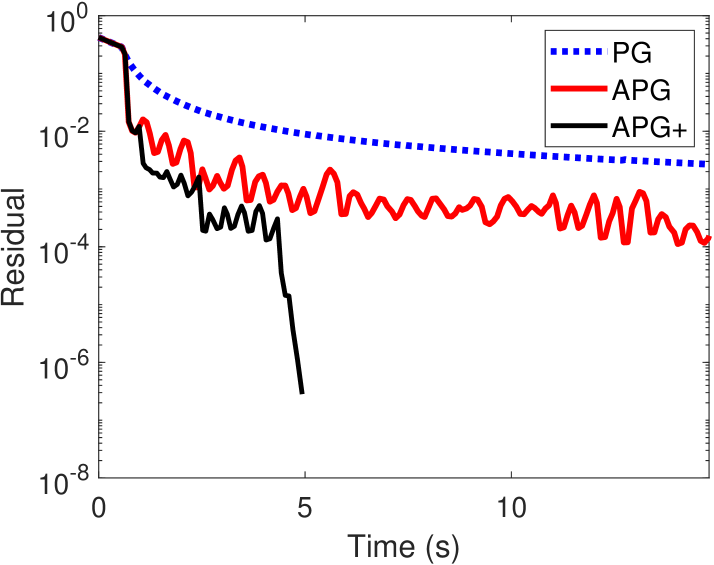
(a) news20, $s=\lceil 0.01m\rceil$

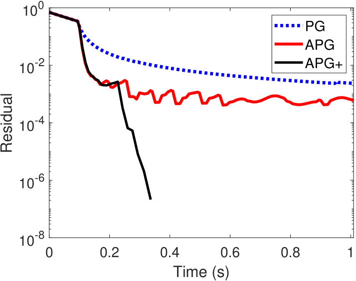
(b) rcv1.binary, $s=\lceil 0.01m\rceil$

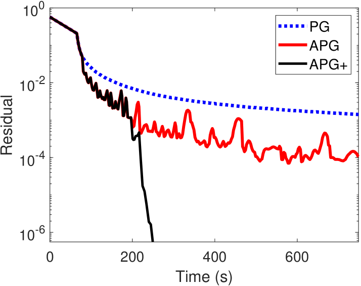
(c) webspam, $s=\lceil 0.001m\rceil$

Least square

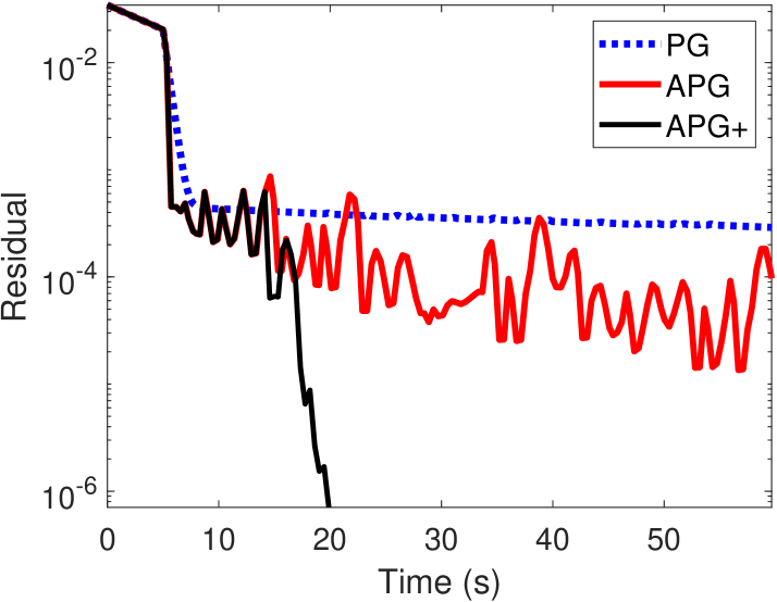
(d) E2006-log1p, $s=\lceil 0.01m\rceil$

(e) E2006-tfidf, $s=\lceil 0.01m\rceil$

Figure 1: Experiment on sparse regularized LR and LS. We present time v.s. residual in Equation 24.

Table 1: Comparison of algorithms for Equation 1 to meet Equation 24 with $\hat{\epsilon}=10^{-6}$, with Equation 23 and Equation 3 and with sparsity levels $s_{1}=\lceil 0.01m\rceil$ and $s_{2}=\lceil 0.05m\rceil$ for all datasets except webspam where $s_{1}=\lceil 0.001m\rceil$ and $s_{2}=\lceil 0.005m\rceil$. CPU: CPU time in seconds. GE: number of gradient evaluations. In one iteration, PG, APG, and APG+ needs one gradient evaluation , while PG-LL and PG-LL+ needs two. CG: number of Hessian-vector products in the PCG procedure for obtaining SSN steps. PA: prediction accuracy (for Equation 23). MSE: mean-squared error (for Equation 3). Time with $*$ indicates that the algorithm is terminated after running $10000$ iterations without satisfying Equation 24.

Dataset	Method	$s_{1}$				$s_{2}$
		CPU	GE	CG	PA	CPU	GE	CG	PA
news20	PG	$*$738.7	10000	0	0.877	$*$728.9	10000	0	0.935
	APG	151.7	1583	0	0.877	758.3	8428	0	0.923
	APG+	5.0	52	63	0.853	16.1	171	67	0.923
	PG-LL	366.7	4682	0	0.873	$*$1494.4	20000	0	0.922
	APG-LL+	6.6	152	88	0.854	29.2	417	89	0.920

rcv1.binary & PG $*$58.4 10000 0 0.937 $*$72.7 10000 0 0.951 APG 12.6 1120 0 0.935 82.4 6372 0 0.934 APG+ 0.3 21 42 0.931 2.4 192 138 0.940 PG-LL 22.2 3638 0 0.935 72.1 8738 0 0.929 APG-LL+ 0.6 99 49 0.930 4.9 626 236 0.939 webspam PG $*$18660.1 10000 0 0.964 $*$30776.2 10000 0 0.978 APG 19683.4 7682 0 0.981 7722.4 2008 0 0.991 APG+ 248.3 75 88 0.969 695.4 164 57 0.991 PG-LL 9001.3 4720 0 0.972 10163.5 3098 0 0.990 APG-LL+ 447.3 264 92 0.965 837.3 294 90 0.992    CPU       GE       CG       MSE       CPU       GE       CG       MSE    E2006-log1p PG $*$2998.6 10000 0 0.167 $*$3644.1 10000 0 0.161 APG 270.6 669 0 0.136 811.8 1757 0 0.133 APG+ 19.5 40 49 0.141 105.6 222 124 0.132 PG-LL $*$6049.8 20000 0 0.132 2696.0 7086 0 0.132 APG-LL+ 41.2 142 38 0.142 107.5 326 100 0.138 E2006-tfidf PG $*$242.7 10000 0 0.152 $*$666.9 10000 0 0.152 APG 1.3 14 0 0.154 3.3 33 0 0.153 APG+ 1.3 8 6 0.141 3.3 31 7 0.139 PG-LL 110.6 4440 0 0.152 304.8 4558 0 0.151 APG-LL+ 1.7 34 6 0.141 3.7 47 7 0.139

Evidently, the extrapolation procedure in APG provides a significant improvement in the running time compared with the base algorithm PG, and further incorporating subspace identification as in APG+ results to a very fast algorithm that outperforms PG and APG by magnitudes. Since the per-iteration cost of PG and APG are almost the same as argued in Section 3, we note that the convergence of APG in terms of iterations is also superior to that of PG.

We next compare APG and APG+ with the extrapolated PG algorithm of Li and Lin [27] that we implement in MATLAB and denote by PG-LL, which is a state-of-the-art approach for nonconvex regularized optimization and thus suitable for Equation 1. We report the required time and number of gradient evaluations (which is the main computation at each iteration) for the algorithms to drive Equation 24 below $\hat{\epsilon}=10^{-6}$. For PG, APG, and APG+, one gradient evaluation is needed per iteration, so the number of gradient evaluations is equivalent to the iteration count. For PG-LL, two gradient evaluations are needed per iteration, so its cost is twice of other methods. We also report the prediction performance on the test data, and we in particular use the test accuracy for Equation 23 and the mean-squared error for Equation 3. Results for the two smaller $s$ are in Section 4 while that for the largest $s$ is in Appendix C. It is clear from the results in Section 4 that APG outperforms PG-LL for most of the test instances considered, while APG+ is magnitudes faster than PG-LL. When we equip PG-LL with our acceleration techniques by replacing $T_{\rm PG}^{\lambda}$ in Algorithms 1 and 2 with the algorithmic map defining PG-LL, we can further speed up PG-LL greatly as shown under the name APG-LL+. We do not observe a method that consistently possesses the best prediction performance, as this is mainly affected by which local optima is found, while no algorithm is able to find the best local optima among all candidates. With no prediction performance degradation, we see that APG+ and APG-LL+ reduce the time needed to solve Equation 1 to a level significantly lower than that of the state of the art.

In Section C.3, we demonstrate the effect on prediction performance when we vary the residual Equation 24 and illustrate that tight residual level is indeed required to obtain better prediction. Comparisons with a greedy method is shown in Section C.4.

Transition Plots.

To demonstrate the behavior of the algorithm for increasing values of $s$, we fit the smaller datasets in Table 3 using logistic loss Equation 23 and least squares loss Equation 3 for varying $s=\lceil km\rceil$, where $k=0.2,0.4,0.6,\dots,3$. The transition plots are presented in Figure 2. We note that the time is in log scale.

We can see clearly that APG+ and APG-LL+ are consistently magnitudes faster than the baseline PG method throughout all sparsity levels. On the other hand, the same-subspace extrapolation scheme of APG is consistently faster than PG and APG-LL and slower than the two Newton acceleration schemes, although the performance is sometimes closer to APG+/APG-LL+ while sometimes closer to PG. APG-LL tends to outperform PG in most situations as well, but in several cases when solving the least square problem, especially when $s$ is small, it can sometimes be slower than PG. Overall speaking, the results in the transition plots show that our proposed acceleration schemes are indeed effective for all sparsity levels tested.

Sparse regularized logistic regression
Sparse least squares regression

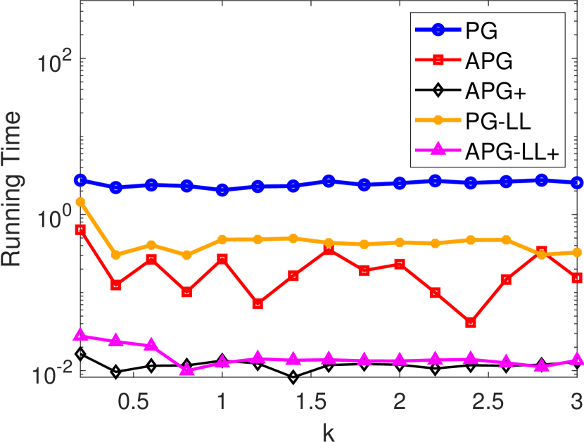
(f) colon-cancer

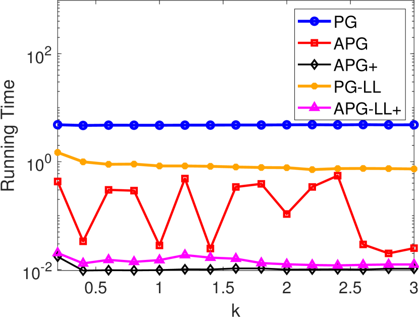
(g) duke

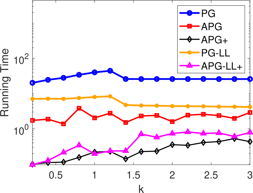
(h) gisette_scale

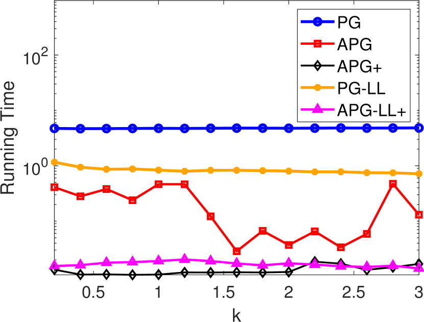
(i) leukemia

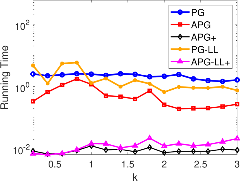
(j) colon-cancer

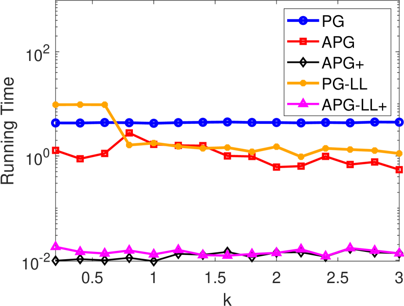
(k) duke

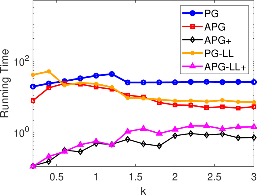
(l) gisette_scale

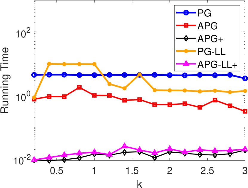
(m) leukemia

Figure 2: Transition plots. We present sparsity levels versus running time (in log scale). Top row: logistic loss. Bottom row: least square loss.

5 Conclusions

In this work, we revisited the projected gradient algorithm for solving $\ell_{0}$-norm constrained optimization problems. Through a natural decomposition of the constraint set into subspaces and the proven ability of the projected gradient method to identify a subspace that contains a solution, we further proposed effective acceleration schemes with provable convergence speed improvements. Experiments showed that our acceleration strategies improve significantly both the convergence speed and the running time of the original projected gradient algorithm, and outperform the state of the art for $\ell_{0}$-norm constrained problems by a huge margin. We plan to extend our analysis and algorithm to the setting of a nonconvex objective in the near future.

Acknowledgments

This work was supported in part by Academia Sinica Grand Challenge Program Seed Grant No. AS-GCS-111-M05 and NSTC of R.O.C. grants 109-2222-E-001-003 and 111-2628-E-001-003.

atoc0

Appendices

Appendix A Implementation Details for Section 3.2

We first discuss our implementation for obtaining inexact SSN steps described in Section 3.2. Given any $w\in A_{J}$, We use the notation $f_{J}(w_{J})\coloneqq f(w)$ to denote the function of considering only the coordinates of $w$ in $J$ as variables and treating the remaining as constants equal to zero. For any $p\in\Re^{s}$, we use $P^{-1}_{A_{J}}$ to denote the vector $\hat{p}\in\Re^{n}$ with $\hat{p}_{J}=p$ and $\hat{p}_{i}=0$ for $i\notin J$. Note that since $f_{J}$ is Lipschitz-continuously differentiable, a generalized Hessian $\nabla^{2}f_{J}$ always exists [19]. When the set of generalized Hessian is not a singleton, we can pick any element in the set.

In large-scale problems often faced in modern machine learning tasks, $s$ can be large even if $s\ll n$, and thus forming the generalized Hessian explicitly and inverting it could still be prohibitively expensive even if we only consider the generalized Hessian in the $s$-dimensional subspace. Therefore, we resort to PCG that, given a preconditioner $M$, iteratively uses the matrix-vector products $\nabla^{2}f_{J}(w_{J})v$ and $M^{-1}u$ for given vectors $u,v\in\Re^{s}$, which can be of much lower cost especially if $M$ has certain structures to facilitate the inverse. Details of PCG can be found in, for instance, Nocedal and Wright [32, Chapter 7]. The PCG approach provides an approximate solution to

$$p\approx\nabla^{2}f_{J}(w_{J})^{-1}\nabla f_{J}(w_{J}),$$

or equivalently,

$$p\approx\operatorname*{arg\,min}_{\bar{p}}\left(Q_{J}(\bar{p};w_{J})\coloneqq\left\langle\nabla f_{J}(w_{J}),\bar{p}\right\rangle+\frac{1}{2}\left\langle\bar{p},\nabla^{2}f_{J}(w_{J})\bar{p}\right\rangle\right).$$ (25)

In our implementation, inspired by the approach of [21], we select the diagonal entries of $\nabla^{2}f_{J}$ as our preconditioner $M$, which provides better performance in our preliminary test over using no preconditioner (or equivalently, taking $M$ as the identity matrix). As this choice of $M$ is a diagonal matrix, its inverse can be computed efficiently in $O(s)$ time.

After obtaining $p$, given parameters $\beta,\sigma_{2}\in(0,1)$, we conduct a backtracking line search procedure to find the largest nonnegative integer $i$ such that

$$f_{J}\left(w_{J}+\beta^{i}p\right)\leq f_{J}\left(w_{J}\right)+\sigma_{2}\beta^{i}\left\langle\nabla f_{J}\left(w_{J}\right),p\right\rangle$$ (26)

and set the step size to $\alpha=\beta^{i}$. Finally, the iterate is updated by

$$w_{J}\leftarrow w_{J}+\alpha p.$$

If $\alpha$ is too small, or this decrease condition cannot be satisfied even when $\beta^{i}$ is already extremely small, we discard this SSN step and declare that this smooth optimization part has failed in Algorithm 2.

For the approximation criterion in Equation 25, let the $i$-th iterate of PCG be $p^{(i)}$ and $Q_{i}\coloneqq Q_{J}(p^{(i)};w_{J})$, we follow [16] to terminate PCG either when it reaches $s$ iterations (at which point theoretically it should have found the exact solution of the right-hand side of Equation 25) or when the $i$-th iterate satisfies $i\geq 1$ and

$$\frac{Q_{i}-Q_{i-1}}{\frac{Q_{i}}{i}}\leq\min\left\{0.5,\sqrt{\left\langle\nabla f_{J}(w_{J}),M^{-1}\nabla f_{J}(w_{J})\right\rangle}\right\},$$ (27)

where $Q_{0}\coloneqq Q(0;w_{J})=0$. It has been shown in [16] that such a stopping condition leads to $Q$-superlinear convergence to an optimum of $f_{J}$ when $\nabla f_{J}$ is semismooth and $f$ is strongly convex. In our case that alternates between such an SSN step and a PG step, we will show that with Equation 27, the overall procedure will enjoy superlinear convergence to $w^{*}$ if $\nabla f$ is semismooth around $x^{*}$; see Theorem F.1 for more details.

One concern is that PCG only works when $\nabla^{2}f_{J}$ is positive definite, but our problem class only guarantees that it is positive semidefinite. To safeguard this issue, one can add a multiple of the identity to $\nabla^{2}f_{J}$ as a damping term to make sure the quadratic term is always positive definite. A particularly useful way is to use $c{\left\|{\nabla f_{J}(w_{J})}\right\|}^{\rho}I$ as the damping term for some $c>0$ and $\rho\in(0,1]$ in Equation 27. When $f_{J}$ satisfies a $q$-metric subregularity condition or an error-bound condition, this damping is known to produce a superlinear convergence rate of order $(1+\rho)$ for a range of $q$ following the analysis in [39, 29]. In Theorem F.1, we do not consider any specific scenarios, but just assume that the smooth optimization subroutine involved itself has a superlinear convergence rate, and show that such a rate is still retained when this subroutine is combined with our algorithm. Therefore, discussions of various schemes including truncated Newton, semismooth Newton, and damping, are all compatible with our general framework to obtain superlinear convergence rates.

Appendix B Experimental settings

All experiments are conducted on a machine with 64GB memory and an Intel Xeon Silver 4208 CPU with 8 cores and 2.1GHz. For all algorithms and all experiments, all cores are utilized. The experiment environment runs Ubuntu 20.04 and MATLAB 2021b. For experiments in Section 4, we use public data listed in Tables 2 and 3. For the datasets that do not come with a test set, we manually do a $80/20$ split to obtain a test set.

Table 2: Data statistics.

Dataset	Loss	#training	#features	#test
		instances ($m$)	($n$)	instances
news20	Equation 23	15,997	1,355,191	3,999
rcv1.binary	Equation 23	20,242	47,236	677,399
webspam	Equation 23	280,000	16,609,143	70,000
E2006-log1p	Equation 3	16,087	4,272,227	3,308
E2006-tfidf	Equation 3	16,087	150,360	3,308

Table 3: Data statistics for small datasets.

Dataset	Loss	#training instances ($m$)	#features ($n$)	#test instances
colon-cancer	Equation 3&Equation 23	50	2,000	12
duke	Equation 3&Equation 23	38	7,129	6
gisette_scale	Equation 3&Equation 23	1,000	5,000	6,000
leukemia	Equation 3&Equation 23	38	7,129	34

The parameters used in our implementation are as follows. We use $\mu=10^{-10}$ in Equation 23. For Algorithm 1, $\sigma=0.05$, $\eta=0.5$, ${\epsilon=10^{-20}}$, $\alpha_{\min}=1$, $\alpha_{\max}=100$, $L$ is estimated using MATLAB’s eigs function to approximate the largest eigenvalue of $AA^{\mathsf{T}}$ with tolerance $10^{-3}$, and $\lambda=0.999/L$. In Algorithm 2, we set $t=1$ and $S=5$, while for the PCG and SSN subroutines, we set $\beta=0.5$ and $\sigma_{2}=0.001$.

Appendix C Additional Experiments

This section provides two sets of additional experiments. We first present results of the datasets in Section 4 with different settings of $s$. The second set of additional experiments are on some smaller datasets that are often considered in existing works for the best subset selection problem like [11].

C.1 Other settings of $s$

We present the other two settings of $s$ described in Section 4 in Figures 3 and 4, and the continuation of Section 4 is presented in Section C.1. Additional experiments with the setting of $s>m$ are presented in Sections C.1 and C.1, which further exemplifies the benefits of our proposed acceleration strategies.

Clearly, for the setting of $s_{3}$ as well as $s>m$, our acceleration techniques continue to greatly improve upon existing methods in almost all cases, with the only excepion being webspam with $s>m$. After a thorough check, we found that the reason is that in this setting, due to the high dimensionality of $n$ and that many pieces of $J\in\mathcal{J}_{s}$ can lead to a very low objective value, the subspaces in which each $w^{k}$ lie change very frequently, so our extrapolation barely take place. This is a potential limit of our method, although in practice we observe that for such easier datasets we probably can avoid this problem by setting $s<m$, which would also make the problem much easier to solve in general (note that with $s<m$, the prediction performance on webspam is not improving at all, suggesting that indeed we do not need to consider the more difficult situation of $s<m$).

We also observe that all for $s\geq m$ on E2006-log1p, all accelerated methods experience significantly larger MSE than the base PG method. After a close examination, we find out that all such acceleration methods provide much lower objective value than PG for the minimization problem, indicating that this is merely due to overfitting of the training data, and indeed PG is alway terminated without reaching the prespecified stopping condition for these cases. This indicates that the accelerated methods are actually performing well from the optimization angle, and this overfitting issue is just a matter of parameter selection.

For E2006-tfidf, we see that for all settings of $s$, identification does not show any additional time improvement in the tables, while the figures clearly show that this is due to that this step kicks in at a very late stage when the residual is already very close to $\hat{\epsilon}$, and if we set $\hat{\epsilon}$ to a smaller value, we can expect observable running time difference between APG and APG+.

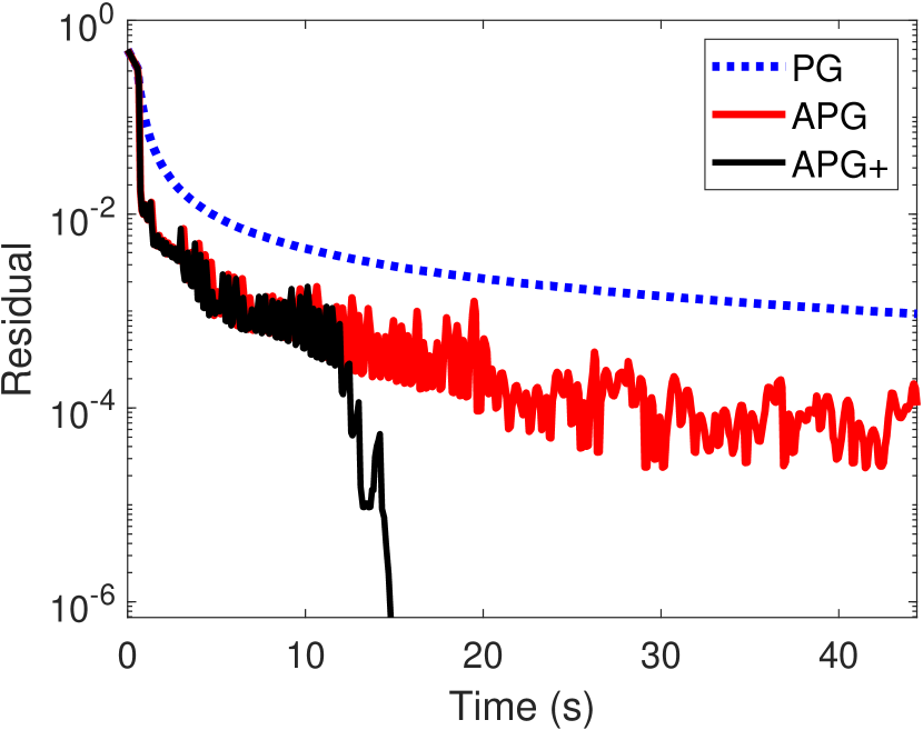
(a) news20, $s=\lceil 0.05m\rceil$

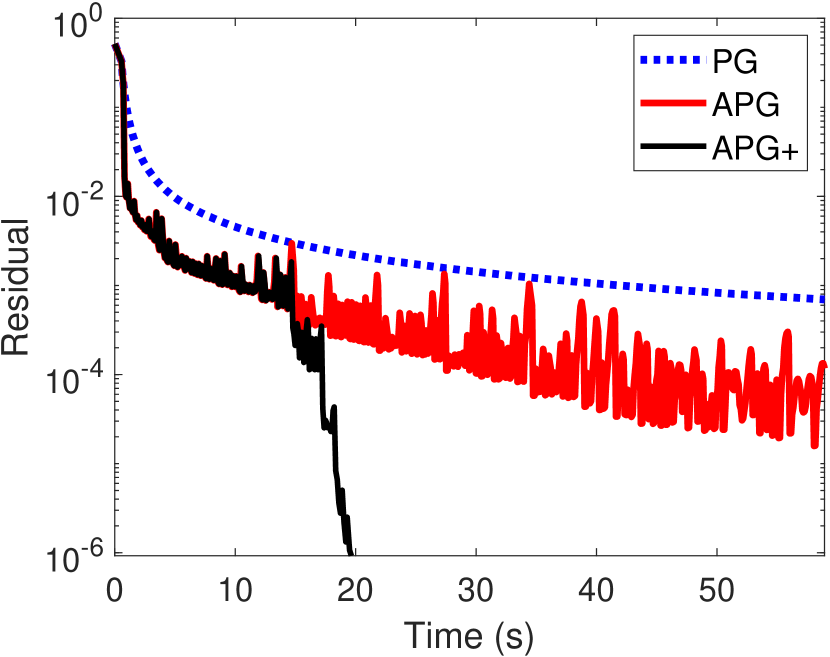
(b) news20, $s=\lceil 0.1m\rceil$

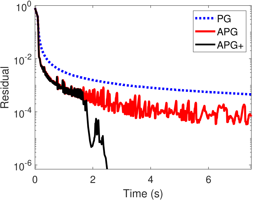
(c) rcv1.binary, $s=\lceil 0.05m\rceil$

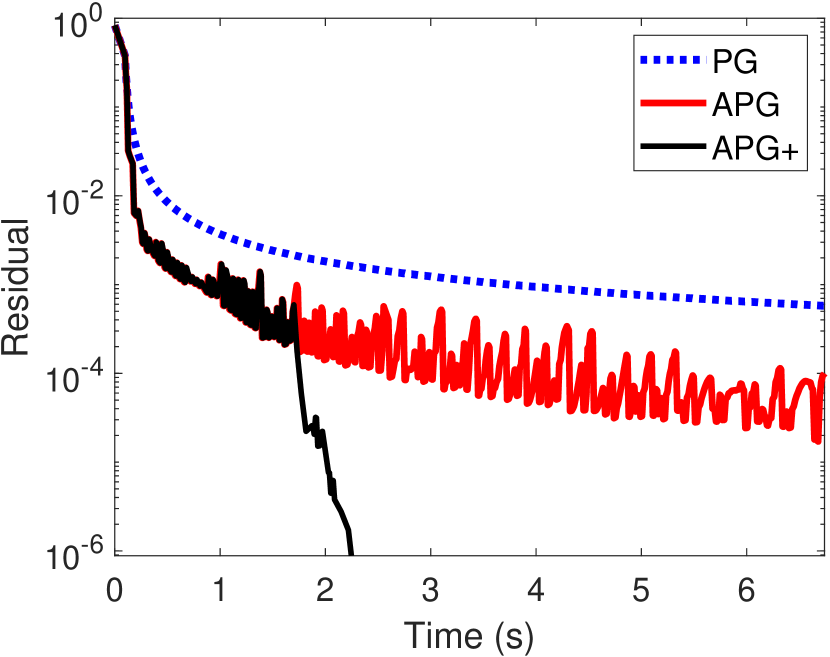
(d) rcv1.binary, $s=\lceil 0.1m\rceil$

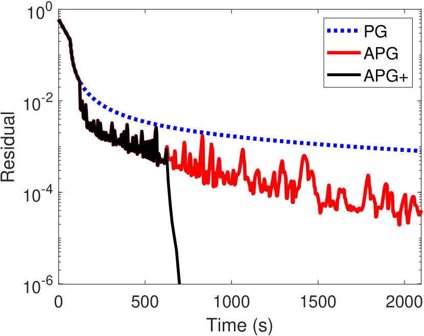
(e) webspam, $s=\lceil 0.005m\rceil$

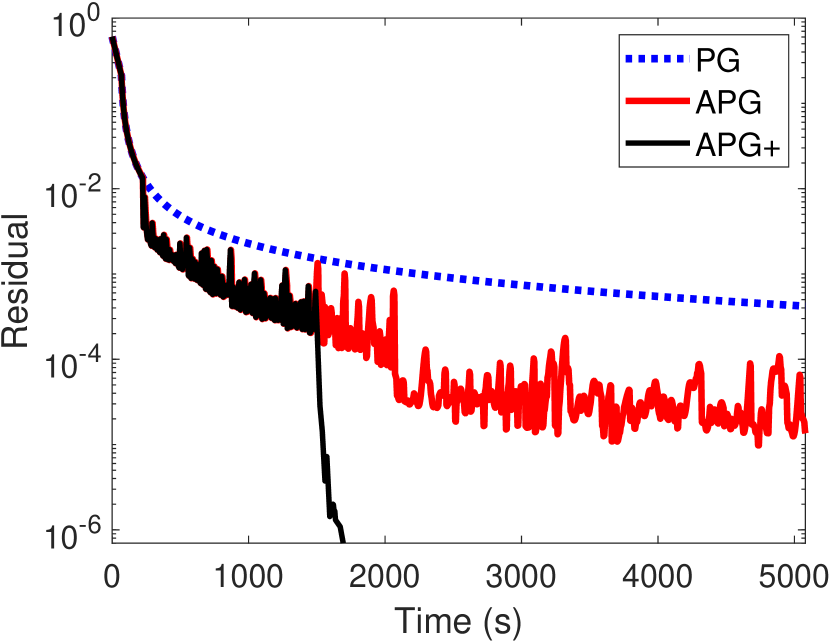
(f) webspam, $s=\lceil 0.01m\rceil$

Figure 3: Sparse regularized logistic loss regression.

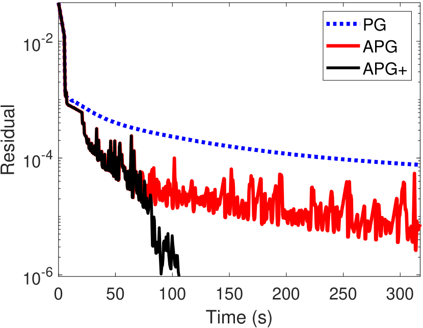
(a) E2006-log1p, $s=\lceil 0.05m\rceil$

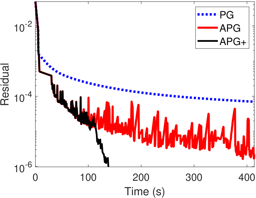
(b) E2006-log1p, $s=\lceil 0.1m\rceil$

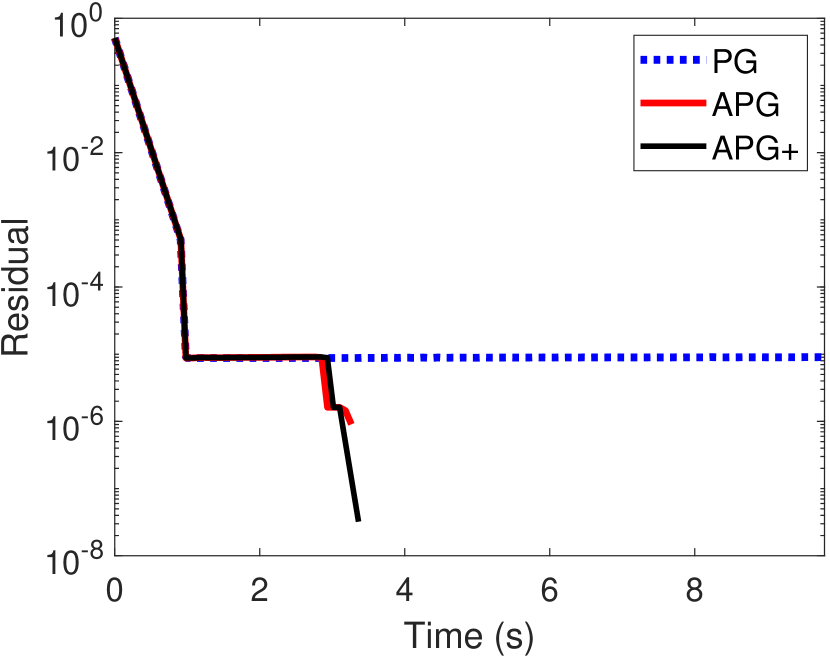
(c) E2006-tfidf, $s=\lceil 0.05m\rceil$

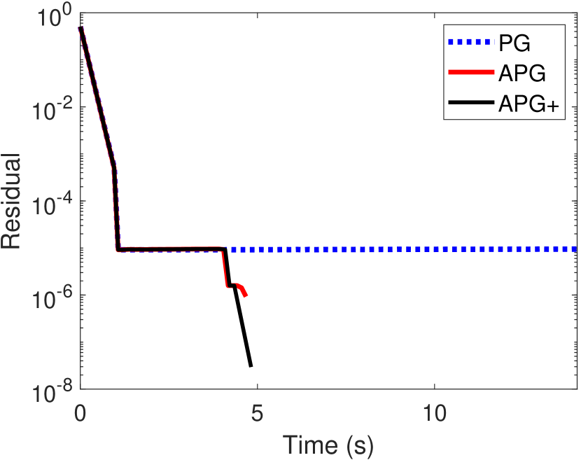
(d) E2006-tfidf, $s=\lceil 0.1m\rceil$

Figure 4: Sparse least squares regression.

Table 4: Comparison of algorithms for Equation 1 to meet Equation 24 with $\hat{\epsilon}<10^{-6}$, with Equation 23 and Equation 3 and with sparsity level $s_{3}=\lceil 0.1m\rceil$ for all datasets except webspam where $s_{3}=\lceil 0.01m\rceil$. CPU: CPU time in seconds. GE: number of gradient evaluations. In one iteration, PG, APG, and APG+ needs one gradient evaluation , while PG-LL and PG-LL+ needs two. CG: number of Hessian-vector products in the PCG procedure for obtaining SSN steps. PA: prediction accuracy (for Equation 23). MSE: mean-squared error (for Equation 3). Time with $*$ indicates that the algorithm is terminated after running $10000$ iterations without satisfying Equation 24.

& PG $*$81.2 10000 0 0.953 APG 33.6 2556 0 0.943 APG+ 2.2 173 93 0.936 PG-LL 21.0 2292 0 0.940 APG-LL+ 4.5 542 106 0.933 webspam PG $*$42487.5 10000 0 0.980 APG 11215.1 2242 0 0.993 APG+ 1664.7 313 83 0.994 PG-LL 14203.9 3176 0 0.992 APG-LL+ 1565.3 367 61 0.994 Dataset Method    $s_{3}$       CPU       GE       CG       MSE    E2006-log1p PG $*$4162.7 10000 0 0.160 APG 559.9 1084 0 0.142 APG+ 138.8 252 122 0.141 PG-LL 1996.5 4532 0 0.141 APG-LL+ 262.5 601 81 0.139 E2006-tfidf PG $*$1086.3 10000 0 0.152 APG 4.7 33 0 0.153 APG+ 4.7 31 7 0.139 PG-LL 512.3 4602 0 0.151 APG-LL+ 8.6 75 7 0.139

Table 5: Comparison of algorithms for Equation 1 to meet Equation 24 with $\hat{\epsilon}=10^{-6}$, with Equation 23 and Equation 3 and with sparsity levels $s\in\{m,\lceil 1.1m\rceil\}$, i.e. $s\geq m$. CPU: CPU time in seconds. GE: number of gradient evaluations. In one iteration, PG, APG, and APG+ needs one gradient evaluation , while PG-LL and PG-LL+ needs two. CG: number of Hessian-vector products in the PCG procedure for obtaining SSN steps. PA: prediction accuracy (for Equation 23). MSE: mean-squared error (for Equation 3). Time with $*$ indicates that the algorithm is terminated after running $10000$ iterations without satisfying Equation 24. Time with $\dagger$ indicates that the algorithm is terminated after exceeding 12 hours of running time without satisfying Equation 24.

& PG $*$81.9 10000 0 0.959 $*$82.6 10000 0 0.959 APG 22.6 1859 0 0.956 18.5 1575 0 0.956 APG+ 5.1 468 47 0.952 5.4 524 47 0.953 PG-LL 15.7 1780 0 0.955 16.0 1784 0 0.955 APG-LL+ 4.9 539 29 0.951 4.6 490 38 0.951 webspam PG $\dagger$43206.6 3902 0 0.977 $\dagger$43203.1 3870 0 0.977 APG $\dagger$43207.8 3866 0 0.985 $\dagger$43202.0 3852 0 0.982 APG+ $\dagger$43207.5 3846 0 0.986 $\dagger$43210.9 3879 0 0.983 PG-LL 35753.0 3190 0 0.995 35776.4 3190 0 0.995 APG-LL+ 36561.7 3190 0 0.995 36494.1 3190 0 0.995    CPU       GE       CG       MSE       CPU       GE       CG       MSE    E2006-log1p PG $*$7039.7 10000 0 0.155 $*$7172.7 10000 0 0.155 APG 4588.4 5819 0 0.207 5011.5 6275 0 0.213 APG+ 1050.0 1362 169 0.344 1320.0 1696 172 0.375 PG-LL 2261.4 3046 0 0.238 2292.0 3040 0 0.238 APG-LL+ 1220.1 1725 171 0.380 1282.3 1751 111 0.340 E2006-tfidf PG $*$1821.0 10000 0 0.152 $*$1819.9 10000 0 0.152 APG 67.4 353 0 0.155 69.0 363 0 0.155 APG+ 67.8 351 8 0.151 69.4 361 8 0.151 PG-LL 906.8 4832 0 0.151 909.6 4836 0 0.151 APG-LL+ 69.3 370 8 0.148 72.8 384 0 0.154

Table 6: Comparison of algorithms for Equation 1 to meet Equation 24 with $\hat{\epsilon}=10^{-6}$, with Equation 23 and Equation 3 and with sparsity levels $s\in\{\lceil 1.5m\rceil,\lceil 2m\rceil\}$, i.e. $s>m$. CPU: CPU time in seconds. GE: number of gradient evaluations. In one iteration, PG, APG, and APG+ needs one gradient evaluation , while PG-LL and PG-LL+ needs two. CG: number of Hessian-vector products in the PCG procedure for obtaining SSN steps. PA: prediction accuracy (for Equation 23). MSE: mean-squared error (for Equation 3). Time with $*$ indicates that the algorithm is terminated after running $10000$ iterations without satisfying Equation 24. Time with $\dagger$ indicates that the algorithm is terminated after exceeding 12 hours of running time without satisfying Equation 24.

& PG $*$84.8 10000 0 0.959 $*$87.8 10000 0 0.959 APG 19.6 1554 0 0.954 15.9 1317 0 0.955 APG+ 4.4 412 42 0.953 4.7 442 59 0.949 PG-LL 16.2 1784 0 0.956 16.6 1786 0 0.956 APG-LL+ 4.7 512 22 0.952 5.5 562 14 0.952 webspam PG $\dagger$43201.3 3809 0 0.977 $\dagger$43207.9 3807 0 0.977 APG $\dagger$43203.8 3815 0 0.978 $\dagger$43201.7 3792 0 0.983 APG+ $\dagger$43202.7 3828 0 0.978 $\dagger$43205.0 3783 0 0.983 PG-LL 36340.5 3190 0 0.995 36325.1 3190 0 0.995 APG-LL+ 36380.0 3190 0 0.995 31177.7 2716 24 0.995    CPU       GE       CG       MSE       CPU       GE       CG       MSE    E2006-log1p PG $*$7617.3 10000 0 0.154 $*$8003.0 10000 0 0.154 APG 5686.2 6781 0 0.209 6375.8 7300 0 0.201 APG+ 1697.5 2104 118 0.279 2098.5 2496 108 0.280 PG-LL 2398.6 3002 0 0.231 2460.1 2946 0 0.225 APG-LL+ 1362.7 1744 94 0.313 1672.1 2057 101 0.299 E2006-tfidf PG $*$1870.2 10000 0 0.152 $*$1894.5 10000 0 0.152 APG 89.0 465 0 0.155 97.0 500 0 0.155 APG+ 89.5 463 8 0.153 97.2 498 8 0.155 PG-LL 927.8 4848 0 0.151 948.6 4856 0 0.151 APG-LL+ 72.8 382 8 0.151 75.0 390 8 0.153

C.2 Experiments with smaller datasets

We now consider some other smaller datasets shown in Table 3, which are also downloaded from the LIBSVM website. Note that for gisette_scale, we interchanged the training and the test sets to make $m<n$. For the setting of $s<m$, we consider $s\in\{\lceil 0.01m\rceil,\lceil 0.05m\rceil,\lceil 0.1m\rceil,\lceil 0.5m\rceil\}$, while for the setting of $s\geq m$, we consider $s\in\{m,\lceil 1.1m\rceil,\lceil 1.5m\rceil,2m\}$. The results of least-square loss in Equation 3 are shown in Sections C.2 and C.2, while the results of the logistic loss in Equation 23 are shown in Sections C.2 and C.2.

We can clearly see from these results that our acceleration schemes are also effective on smaller datasets to reduce the running time to magnitudes shorter. However, there are several cases that the running time is too short such that the digits in the tables are unable to show difference between APG and APG+. We do not try to increase the number of digits in such cases, as the running time is anyway already extremely short, and the difference would not make much difference for problems that can be solved with such high efficiency.

Table 7: Comparison of algorithms for Equation 1 to meet Equation 24 with $\hat{\epsilon}=10^{-6}$, with Equation 3 with sparsity levels $s\in\{\lceil 0.01m\rceil,\lceil 0.05m\rceil,\lceil 0.1m\rceil,\lceil 0.5m\rceil\}$. CPU: CPU time in seconds. GE: number of gradient evaluations. In one iteration, PG, APG, and APG+ needs one gradient evaluation , while PG-LL and PG-LL+ needs two. CG: number of Hessian-vector products in the PCG procedure for obtaining SSN steps. MSE: mean-squared error (for Equation 3). Time with $*$ indicates that the algorithm is terminated after running $10000$ iterations without satisfying Equation 24.

& PG $*$4.07 10000 0 1.568 $*$4.18 10000 0 1.145 APG 0.01 5 0 1.581 0.01 8 0 1.140 APG+ 0.01 5 0 1.581 0.01 8 2 1.140 PG-LL 0.19 382 0 1.579 0.75 1514 0 1.141 APG-LL+ 0.01 10 0 1.581 0.01 16 2 1.140 gisette_scale PG $*$13.35 10000 0 0.465 $*$14.70 10000 0 0.304 APG 4.08 1526 0 0.464 3.63 1286 0 0.303 APG+ 0.07 11 18 0.464 0.08 13 38 0.334 PG-LL 2.45 1758 0 0.466 $*$30.15 20000 0 0.268 APG-LL+ 0.07 32 18 0.464 0.08 37 23 0.337 leukemia PG 3.67 8768 0 0.595 2.80 6726 0 0.566 APG 0.01 5 0 0.595 0.01 8 0 0.566 APG+ 0.01 5 0 0.595 0.01 8 2 0.566 PG-LL 0.14 302 0 0.595 0.77 1632 0 0.566 APG-LL+ 0.01 10 0 0.595 0.01 16 2 0.566 Dataset Method    $s=\lceil 0.1m\rceil$       $s=\lceil 0.5m\rceil$       CPU       GE       CG       MSE       CPU       GE       CG       MSE    colon-cancer PG 1.59 6951 0 0.652 $*$2.51 10000 0 1.855 APG 0.13 320 0 0.599 1.48 3268 0 2.461 APG+ 0.01 10 10 0.599 0.02 18 27 1.345 PG-LL 0.52 2990 0 0.656 $*$6.26 20000 0 1.895 APG-LL+ 0.01 24 10 0.599 0.02 61 31 1.723 duke PG $*$4.28 10000 0 0.860 $*$4.18 10000 0 0.864 APG 0.02 23 0 0.882 1.26 1749 0 0.569 APG+ 0.01 9 5 0.882 0.01 11 14 1.060 PG-LL 0.84 1670 0 0.880 1.05 2284 0 1.089 APG-LL+ 0.02 19 5 0.882 0.01 28 14 1.060 gisette_scale PG $*$15.63 10000 0 0.243 $*$23.63 10000 0 0.220 APG 7.83 2697 0 0.212 14.97 3922 0 0.292 APG+ 0.08 13 41 0.260 0.22 43 108 0.253 PG-LL 5.37 3294 0 0.238 $*$50.85 20000 0 0.364 APG-LL+ 0.09 54 40 0.259 0.48 271 149 0.258 leukemia PG $*$4.35 10000 0 0.523 $*$4.47 10000 0 0.582 APG 0.99 1263 0 0.524 0.63 876 0 1.277 APG+ 0.01 9 5 0.524 0.01 10 16 1.676 PG-LL 0.93 1966 0 0.524 $*$9.79 20000 0 1.226 APG-LL+ 0.01 19 5 0.524 0.01 30 16 1.676

Table 8: Comparison of algorithms for Equation 1 to meet Equation 24 with $\hat{\epsilon}=10^{-6}$, with Equation 3 with sparsity levels $s\in\{m,\lceil 1.1m\rceil,\lceil 1.5m\rceil,2m\}$. CPU: CPU time in seconds. GE: number of gradient evaluations. In one iteration, PG, APG, and APG+ needs one gradient evaluation , while PG-LL and PG-LL+ needs two. CG: number of Hessian-vector products in the PCG procedure for obtaining SSN steps. MSE: mean-squared error (for Equation 3). Time with $*$ indicates that the algorithm is terminated after running $10000$ iterations without satisfying Equation 24.

& PG $*$4.18 10000 0 0.554 $*$4.25 10000 0 0.549 APG 1.42 1945 0 1.531 1.24 1631 0 0.505 APG+ 0.01 13 58 0.209 0.01 11 39 2.061 PG-LL 1.80 3782 0 0.635 1.47 3104 0 0.281 APG-LL+ 0.02 101 87 6.685 0.01 58 44 0.831 gisette_scale PG $*$35.83 10000 0 0.226 $*$40.06 10000 0 0.225 APG 16.50 3326 0 0.298 15.55 3000 0 0.308 APG+ 0.58 78 247 0.499 1.20 200 203 0.347 PG-LL 21.09 5364 0 0.367 18.91 4462 0 0.359 APG-LL+ 0.99 330 144 0.341 1.59 449 203 0.508 leukemia PG $*$4.22 10000 0 0.649 $*$4.30 10000 0 0.703 APG 1.05 1202 0 0.967 1.06 1445 0 0.980 APG+ 0.02 15 104 4.722 0.02 17 98 9.202 PG-LL $*$9.64 20000 0 1.050 1.87 3968 0 1.718 APG-LL+ 0.02 118 104 4.722 0.02 112 98 9.202 Dataset Method    $s=\lceil 1.5m\rceil$       $s=2m$       CPU       GE       CG       MSE       CPU       GE       CG       MSE    colon-cancer PG $*$2.71 10000 0 3.277 2.03 8195 0 3.062 APG 0.27 805 0 2.836 0.22 614 0 3.016 APG+ 0.02 27 79 3.092 0.02 42 44 3.131 PG-LL 3.52 14734 0 3.016 0.66 3024 0 2.964 APG-LL+ 0.03 139 67 3.279 0.03 123 63 3.032 duke PG $*$4.30 10000 0 0.392 $*$4.28 10000 0 0.333 APG 0.84 1162 0 0.271 0.51 687 0 0.301 APG+ 0.01 13 40 0.259 0.01 12 33 0.564 PG-LL 1.79 3740 0 0.373 1.49 2990 0 0.539 APG-LL+ 0.02 48 34 0.308 0.02 47 33 0.564 gisette_scale PG $*$23.09 10000 0 0.230 $*$23.08 10000 0 0.237 APG 7.40 2057 0 0.284 5.03 1443 0 0.282 APG+ 0.52 118 133 0.339 1.32 357 143 0.319 PG-LL 7.88 3242 0 0.347 6.98 2860 0 0.328 APG-LL+ 1.15 500 150 0.387 1.13 488 128 0.336 leukemia PG $*$4.36 10000 0 0.730 $*$4.30 10000 0 0.704 APG 0.69 865 0 0.694 0.47 574 0 0.619 APG+ 0.02 19 53 1.369 0.01 12 42 0.944 PG-LL 1.92 3952 0 1.074 1.38 2862 0 0.714 APG-LL+ 0.03 81 49 1.230 0.01 43 29 0.926

Table 9: Comparison of algorithms for Equation 1 to meet Equation 24 with $\hat{\epsilon}=10^{-6}$, with Equation 23 with sparsity levels $s\in\{\lceil 0.01m\rceil,\lceil 0.05m\rceil,\lceil 0.1m\rceil,\lceil 0.5m\rceil\}$. CPU: CPU time in seconds. GE: number of gradient evaluations. In one iteration, PG, APG, and APG+ needs one gradient evaluation , while PG-LL and PG-LL+ needs two. CG: number of Hessian-vector products in the PCG procedure for obtaining SSN steps. PA: prediction accuracy (for Equation 23). Time with $*$ indicates that the algorithm is terminated after running $10000$ iterations without satisfying Equation 24.

& PG $*$4.52 10000 0 0.000 $*$4.72 10000 0 0.500 APG 0.01 11 0 0.000 0.01 12 0 0.500 APG+ 0.01 8 1 0.000 0.01 8 2 0.500 PG-LL 0.47 958 0 0.000 0.58 1038 0 0.500 APG-LL+ 0.01 15 1 0.000 0.01 16 2 0.500 gisette_scale PG $*$16.11 10000 0 0.839 $*$17.50 10000 0 0.912 APG 11.62 3600 0 0.888 6.81 1980 0 0.916 APG+ 0.07 10 15 0.851 0.08 11 23 0.900 PG-LL $*$34.11 20000 0 0.863 5.34 2780 0 0.916 APG-LL+ 0.08 29 15 0.851 0.09 38 24 0.898 leukemia PG $*$4.60 10000 0 0.824 $*$4.81 10000 0 0.882 APG 0.01 9 0 0.824 0.05 46 0 0.853 APG+ 0.01 9 2 0.824 0.01 10 6 0.853 PG-LL 0.81 1612 0 0.824 1.23 2278 0 0.853 APG-LL+ 0.01 16 2 0.824 0.01 20 6 0.853 Dataset Method    $s=\lceil 0.1m\rceil$       $s=\lceil 0.5m\rceil$       CPU       GE       CG       PA       CPU       GE       CG       PA    colon-cancer PG $*$2.48 10000 0 0.833 $*$2.21 10000 0 0.833 APG 2.51 3651 0 0.833 0.20 255 0 0.833 APG+ 0.02 11 12 0.833 0.02 14 55 0.833 PG-LL $*$5.79 20000 0 0.833 0.29 1376 0 0.833 APG-LL+ 0.02 29 15 0.833 0.02 58 44 0.833 duke PG $*$4.71 10000 0 0.750 $*$4.81 10000 0 0.750 APG 0.03 33 0 0.500 0.43 431 0 0.750 APG+ 0.01 10 8 0.500 0.01 11 11 0.750 PG-LL 1.22 2352 0 0.500 0.99 1800 0 0.750 APG-LL+ 0.01 22 8 0.500 0.02 25 11 0.750 gisette_scale PG $*$18.31 10000 0 0.928 $*$27.24 10000 0 0.951 APG 4.79 1329 0 0.934 2.62 608 0 0.960 APG+ 0.09 12 42 0.923 0.23 48 34 0.956 PG-LL 6.40 3190 0 0.936 7.18 2324 0 0.955 APG-LL+ 0.09 56 42 0.923 0.14 59 45 0.955 leukemia PG $*$4.79 10000 0 0.912 $*$4.81 10000 0 0.912 APG 0.54 522 0 0.824 0.29 304 0 0.882 APG+ 0.01 11 10 0.853 0.01 11 9 0.912 PG-LL 1.50 2726 0 0.912 0.92 1698 0 0.912 APG-LL+ 0.02 21 7 0.853 0.02 24 10 0.912

Table 10: Comparison of algorithms for Equation 1 to meet Equation 24 with $\hat{\epsilon}=10^{-6}$, with Equation 23 with sparsity levels $s\in\{m,\lceil 1.1m\rceil,\lceil 1.5m\rceil,2m\}$. CPU: CPU time in seconds. GE: number of gradient evaluations. In one iteration, PG, APG, and APG+ needs one gradient evaluation , while PG-LL and PG-LL+ needs two. CG: number of Hessian-vector products in the PCG procedure for obtaining SSN steps. PA: prediction accuracy (for Equation 23). Time with $*$ indicates that the algorithm is terminated after running $10000$ iterations without satisfying Equation 24.

& PG $*$4.82 10000 0 0.750 $*$4.81 10000 0 0.750 APG 0.03 31 0 0.750 0.33 351 0 0.500 APG+ 0.01 11 9 0.750 0.01 11 9 0.750 PG-LL 0.81 1558 0 0.750 0.80 1540 0 0.750 APG-LL+ 0.02 23 9 0.750 0.02 23 9 0.750 gisette_scale PG $*$40.08 10000 0 0.956 $*$42.05 10000 0 0.957 APG 1.96 366 0 0.960 3.94 668 0 0.957 APG+ 0.61 102 28 0.962 0.45 69 35 0.962 PG-LL 8.03 1862 0 0.962 8.19 1794 0 0.961 APG-LL+ 0.25 57 33 0.959 0.92 192 28 0.962 leukemia PG $*$4.79 10000 0 0.912 $*$4.75 10000 0 0.912 APG 0.43 439 0 0.971 0.25 265 0 0.912 APG+ 0.01 11 8 0.912 0.02 11 8 0.941 PG-LL 0.83 1538 0 0.912 0.80 1516 0 0.912 APG-LL+ 0.02 22 8 0.912 0.02 22 8 0.941 Dataset Method    $s=\lceil 1.5m\rceil$       $s=2m$       CPU       GE       CG       PA       CPU       GE       CG       PA    colon-cancer PG $*$2.69 10000 0 0.833 $*$2.39 10000 0 0.833 APG 0.09 219 0 0.667 0.23 304 0 0.833 APG+ 0.02 28 25 0.833 0.03 40 20 0.833 PG-LL 0.37 1282 0 0.833 0.30 1298 0 0.833 APG-LL+ 0.02 47 33 0.750 0.02 55 25 0.750 duke PG $*$4.80 10000 0 0.750 $*$4.83 10000 0 0.750 APG 0.04 43 0 0.750 0.11 104 0 0.750 APG+ 0.01 11 9 0.750 0.01 12 11 0.750 PG-LL 0.84 1496 0 0.750 0.81 1416 0 0.750 APG-LL+ 0.02 30 6 0.750 0.02 25 11 0.750 gisette_scale PG $*$26.10 10000 0 0.956 $*$26.29 10000 0 0.956 APG 2.55 583 0 0.958 1.53 365 0 0.944 APG+ 0.48 107 25 0.960 0.69 159 23 0.956 PG-LL 4.66 1658 0 0.958 4.42 1568 0 0.959 APG-LL+ 0.63 193 15 0.960 0.74 242 12 0.958 leukemia PG $*$4.67 10000 0 0.912 $*$4.75 10000 0 0.912 APG 0.44 435 0 0.971 0.03 36 0 0.941 APG+ 0.02 12 11 0.941 0.01 12 11 0.941 PG-LL 0.81 1480 0 0.912 0.78 1406 0 0.941 APG-LL+ 0.02 25 11 0.941 0.02 25 11 0.941

C.3 Prediction accuracy for varying residuals

We present in Figure 5 the effect of varying the tolerance level $\hat{\epsilon}$ for the residual Equation 24. We can clearly see that in all cases, the prediction performance of all methods keeps improving up to $\hat{\epsilon}=10^{-5}$, which indicates that our choice of a rather tight stopping condition is indeed a suitable one for getting better prediction performance. Note that in terms of comparison between different algorithms, the results in Figure 5 are consistent with that in Section 4.

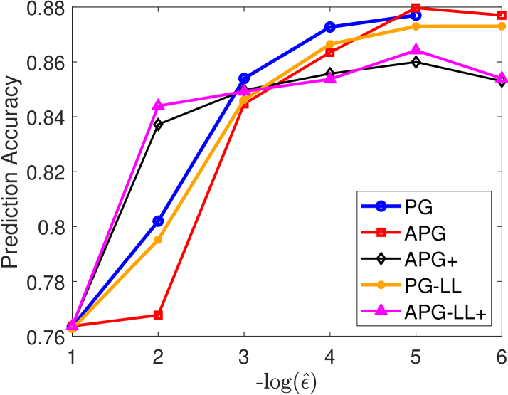
(a) news20

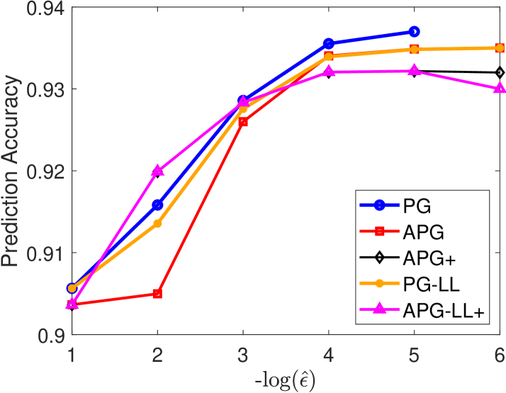
(b) rcv1.binary

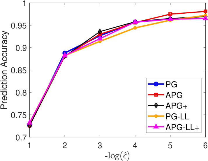
(c) webspam

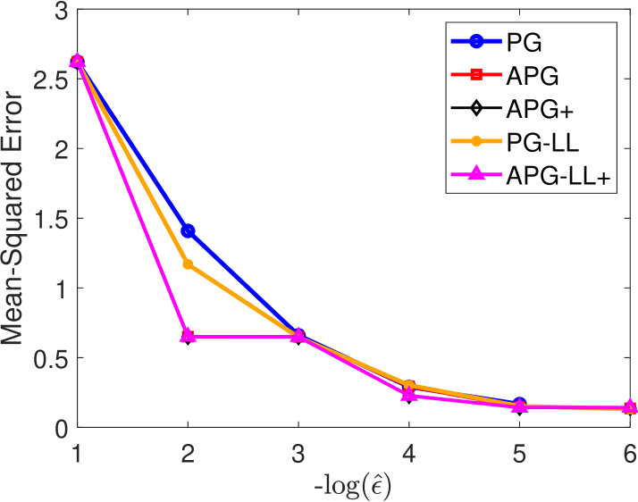
(d) E2006-log1p

Figure 5: Prediction performance of different methods for sparse logistic regression (news20, rcv1.binary, webspam) and least squares regression (E2006-log1p) across varying levels of residuals $\epsilon=10^{-k}$, with $k=1,2,\dots,6$. Generated plots correspond to sparsity level of $s=\lceil 0.01m\rceil$.

C.4 Numerical comparison with a greedy method

We present in Figure 6 results of numerical comparisons of our methods with the GraSP algorithm of Bahmani et al. [3], which is designed to solve our target problem Equation 1 for general loss functions $f$. Each iteration of GraSP involves a restricted minimization problem along a subspace of dimension at most $3s$, which is solved by a quasi-Newton approach. Note that GraSP is not ideal for large-scale datasets for its prohibitive memory consumption. For instance, it failed to fit the webspam dataset even with the smallest sparsity level $s=\lceil 0.001m\rceil$ on our machine with 64GB memory with an out of memory error, whereas our proposed algorithm performs quite well for this instance. For a medium-sized dataset such as news20, we see from Figure 6 that GraSP performs significantly slower than our proposed accelerated algorithm. In particular, its initial convergence is extremely fast, but it then becomes stagnant after reaching a low-to-medium precision.

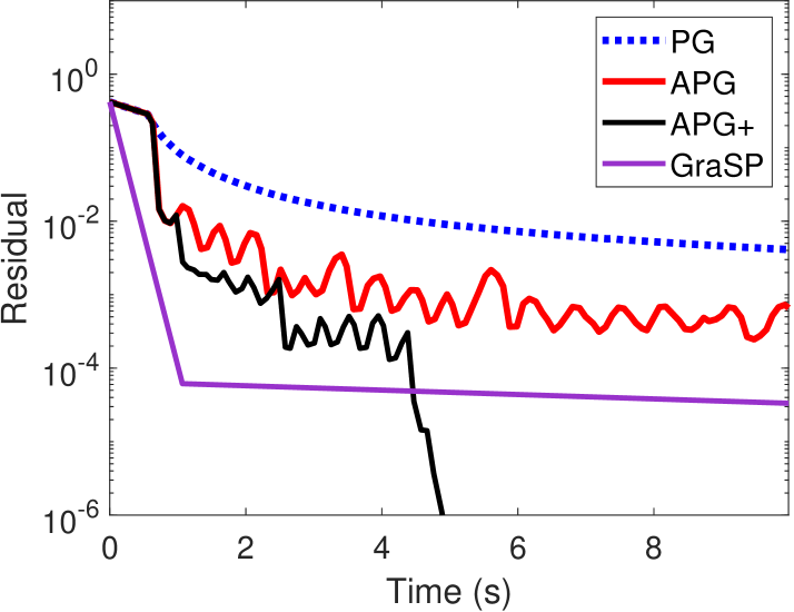
(a) news20, $s=\lceil 0.01m\rceil$

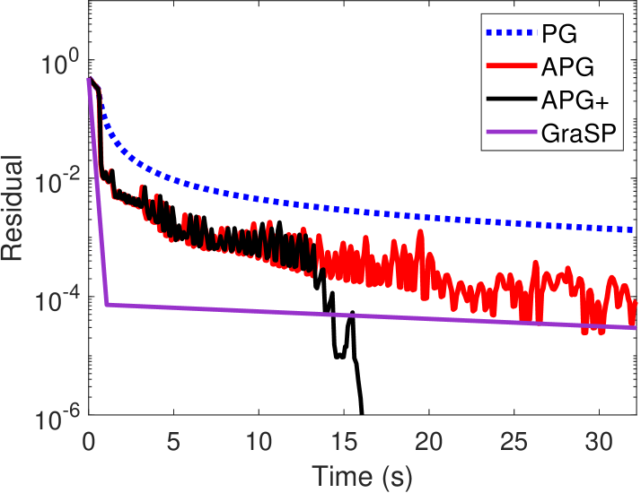
(b) news20, $s=\lceil 0.05m\rceil$

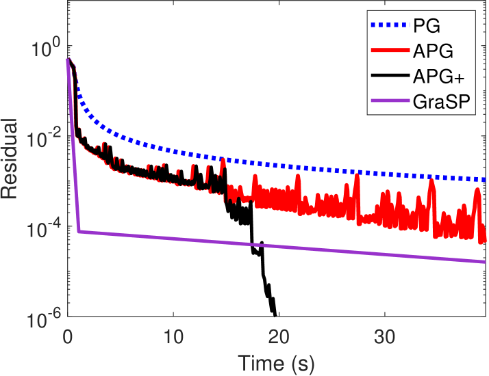
(c) news20, $s=\lceil 0.1m\rceil$

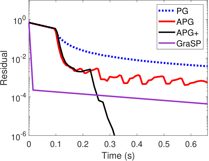
(d) rcv1.binary, $s=\lceil 0.01m\rceil$

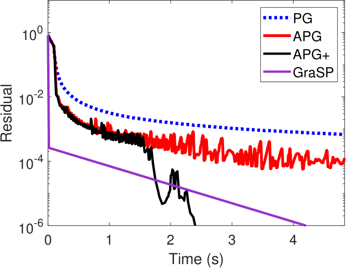
(e) rcv1.binary, $s=\lceil 0.05m\rceil$

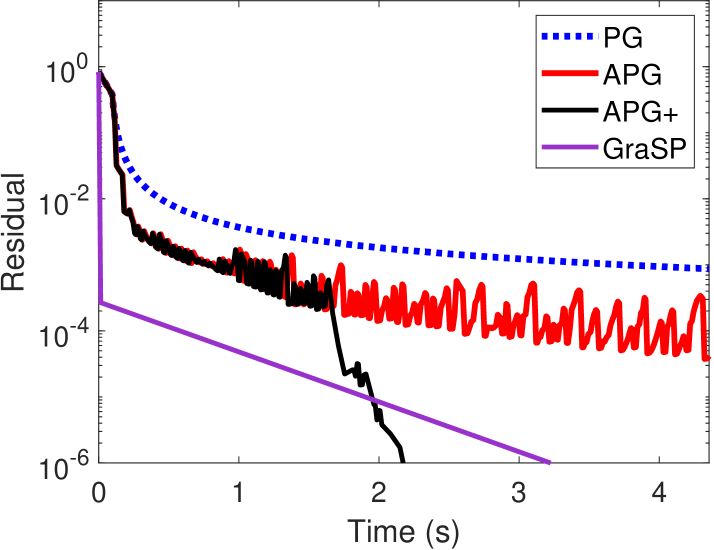
(f) rcv1.binary, $s=\lceil 0.1m\rceil$

Figure 6: Comparison of non-accelerated and accelerated projected gradient methods with GraSP for solving regularized sparse logistic regression.

Appendix D Proofs of Results in Section 2

D.1 Proof of Theorem 2.1

Proof of part (a).

We note that the iterates of Equation 5 are confined to $A_{s}$. Consider any accumulation point $w^{*}$ of $\{w^{k}\}$. For any given convergent subsequence $\{w^{k_{r}}\}$ with $w^{k_{r}}\to w^{*}$, we obtain from the finiteness of $\mathcal{J}_{s}$ that there is $J\in\mathcal{J}_{s}$ such that

$$w^{k_{r}+1}=P_{A_{J}}(w^{k_{r}}-\lambda\nabla f(w^{k_{r}}))$$ (28)

for infinitely many $r$. By taking subsequences if necessary, we assume that Equation 28 holds for all $r$ without loss of generality. Meanwhile, the PG iterates Equation 5 can alternatively be written as

$$w^{k+1}\in\operatorname*{arg\,min}_{y\in A_{s}}~{}\left\langle\nabla f(w^{k}),y-w^{k}\right\rangle+\frac{1}{2\lambda}\|y-w^{k}\|^{2}.$$ (29)

We also use the fact that Equation 6 implies the well-known descent lemma [see for example, 7, Lemma 5.7]

$$f(w)\leq f(w^{\prime})+\left\langle\nabla f(w^{\prime}),w-w^{\prime}\right\rangle+\frac{L}{2}\|w-w^{\prime}\|^{2},\quad\forall w,w^{\prime}\in\Re^{n}.$$ (30)

Noting that $\lambda\in(0,L^{-1})$, we have

$$f(w^{k+1})$$

$$\overset{\lx@cref{creftype~refnum}{eq:descentlemma}}{\leq} f(w^{k})+\left\langle\nabla f(w^{k}),w^{k+1}-w^{k}\right\rangle+\frac{L}{2}\|w^{k+1}-w^{k}\|^{2}$$

$$= f(w^{k})+\left\langle\nabla f(w^{k}),w^{k+1}-w^{k}\right\rangle+\frac{1}{2\lambda}\|w^{k+1}-w^{k}\|^{2}+\left(\frac{\lambda L-1}{2\lambda}\right)\|w^{k+1}-w^{k}\|^{2}$$

$$\overset{\lx@cref{creftype~refnum}{eq:pgm_alternative}}{\leq} f(w^{k})+\left(\frac{\lambda L-1}{2\lambda}\right)\|w^{k+1}-w^{k}\|^{2}.$$

That is,

$$\frac{1-\lambda L}{2\lambda}\|w^{k}-w^{k+1}\|^{2}\leq f(w^{k})-f(w^{k+1}).$$ (31)

If $w^{N}=w^{N+1}$ for some $N$, then it is clear from Equation 31 that $w^{k}=w^{N}$ for all $k\geq N$. Otherwise, $\{f(w^{k})\}$ is strictly decreasing, proving the first claim of part (a). Noting that $\nabla f$ and $P_{A_{J}}$ are continuous as $A_{J}$ is closed and convex, we obtain from Equation 28 that $w^{k_{r}+1}\to P_{A_{J}}(w^{*}-\lambda\nabla f(w^{*}))$ as $r\to\infty$. On the other hand, we see from Equation 31 and the lower boundedness of $f$ that $\|w^{k}-w^{k+1}\|\to 0$, which, by means of the triangle inequality, implies that $w^{k_{r}+1}\to w^{*}$. Hence, we have $w^{*}=P_{A_{J}}(w^{*}-\lambda\nabla f(w^{*}))$. To complete the proof of part (a), we only need to show that $P_{A_{J}}(w^{*}-\lambda\nabla f(w^{*}))\in P_{A_{s}}(w^{*}-\lambda\nabla f(w^{*}))$. But from Equation 28 and Equation 5, we have that for all $r$, $w^{k_{r}}\in D_{J}$, where

$$D_{J}\coloneqq\{z\in\Re^{n}:\operatorname*{dist}(z-\lambda\nabla f(z),A_{J})=\operatorname*{dist}(z-\lambda\nabla f(z),A_{s})\},$$ (32)

where for any point $x$ and any set $A$, $\operatorname*{dist}(x,A)$ is the distance from $x$ to $A$, defined as

$$\operatorname*{dist}(x,A)=\inf_{y\in A}{\left\|{x-y}\right\|}.$$

Since $A_{J}$ is closed, it follows that $D_{J}$ is a closed set as well, and therefore $w^{*}\in D_{J}$. That is, $P_{A_{J}}(w^{*}-\lambda\nabla f(w^{*}))\in P_{A_{s}}(w^{*}-\lambda\nabla f(w^{*}))$, as desired.

Finally, we note that by representing Equation 1 as

$$\min_{w}\quad f(w)+\delta_{A_{s}}(w),$$

where $\delta_{A_{s}}$ is the indicator function of $A_{s}$ that outputs $0$ when $w\in A_{s}$ and infinity otherwise, a point $w^{*}$ is called stationary for Equation 1 if

$$0\in\partial f(w^{*})+\partial\delta_{A_{s}}(w),$$

where $\partial g$ is the limiting subdifferential in the sense of Clarke. On the other hand, the optimality condition of $w^{*}\in P_{A_{s}}(w^{*}-\lambda\nabla f(w^{*}))$ implies that

$$0\in w^{*}-\left(w^{*}-\lambda\nabla f(w^{*})\right)+\partial\delta_{A_{s}}(w^{*})\quad\Leftrightarrow\quad 0\in\lambda\nabla f(w^{*})+\partial\delta_{A_{s}}(w^{*}).$$

Since $\lambda\delta_{A_{s}}=\delta_{A_{s}}$ for any $\lambda$, the result above further implies that

$$\lambda^{-1}0=0\in\nabla f(w^{*})+\partial\delta_{A_{s}}(w^{*}),$$

showing that $w^{*}$ is indeed a stationary point of Equation 1. ∎

Proof of part (b).

Suppose that $w^{k}\to w^{*}$ and define $I_{w^{*}}$ as in Equation 8. The finiteness of $\mathcal{J}_{s}$ implies that there exists $\delta>0$ such that

$$B_{\delta}(w^{*})\cap A_{J}=\emptyset,\quad\forall J\notin I_{w^{*}},$$ (33)

where $B_{\delta}(w^{*})\coloneqq\{w\in\Re^{n}:\|w-w^{*}\|<\delta\}$. Since $w^{k}\to w^{*}$, we can find $N>0$ such that $w^{k}\in B_{\delta}(w^{*})$ for all $k\geq N$. Hence, Equation 8 immediately follows.

Now, suppose that $T_{\rm PG}(w^{*})$ is a singleton for some accumulation point $w^{*}$. Together with Theorem 2.1 (a), we have

$$P_{A_{s}}(w^{*}-\lambda\nabla f(w^{*}))=\{w^{*}\}$$ (34)

It is easy to verify that Equation 34 implies that

$$w^{*}=P_{A_{J}}(w^{*}-\lambda\nabla f(w^{*}))\quad\forall J\in I_{w^{*}}.$$ (35)

That is, $w^{*}$ is a global minimum of $f$ over $A_{J}$ for all $J\in I_{w^{*}}$ due to the convexity of $f$. Now let $\delta>0$ be as defined in the preceding paragraph and $z\in A_{s}\cap B_{\delta}(w^{*})$. It then follows from Equation 33 that $z\in A_{J}$ for some $J\in I_{w^{*}}$ . By the global minimality of $w^{*}$ for $f|_{A_{J}}$, it follows that $f(w^{*})\leq f(z)$ for all $z\in A_{s}\cap B_{\delta}(w^{*})$. That is, $w^{*}$ is a local minimum of $f$ over $A_{s}$.

It remains to show that the full sequence $\{w^{k}\}$ converges to $w^{*}$. To this end, choose $\nu>0$ sufficiently small such that $z\in D_{J}\cap B_{\nu}(w^{*})$ for some $J$ implies $w^{*}\in D_{J}$, where $D_{J}$ is defined as in Equation 32. Note that such a $\nu$ exists as the collection $\{D_{J}:J\in\mathcal{J}_{s}\}$ is finite and consists of closed sets. Let $\{w^{k_{r}}\}_{r=0}^{\infty}$ be a subsequence converging to $w^{*}$. We may assume without loss of generality that $w^{k_{r}}\in B_{\nu}(w^{*})$ for all $r\geq 0$. First, we show that $w^{k_{0}+1}\in B_{\nu}(w^{*})$. Note that the convexity of $f$ and Equation 6 result to nonexpansiveness of the mapping $w\mapsto w-\lambda\nabla f(w)$ because $\lambda\leq L^{-1}$ [7, Theorem 5.8]. From Equation 5, $w^{k_{0}+1}=P_{A_{J}}\left(w^{k_{0}}-\lambda\nabla f(w^{k_{0}})\right)$ for some $J$. By the choice of $\nu$ and the fact that $T_{\rm PG}^{\lambda}(w^{*})$ consists of one element, we see that $w^{*}=P_{A_{J}}(w^{*}-\lambda\nabla f(w^{*}))$. With these, we have

$$\|w^{k_{0}+1}-w^{*}\| =\|P_{A_{J}}\left(w^{k_{0}}-\lambda\nabla f(w^{k_{0}})\right)-P_{A_{J}}(w^{*}-\lambda\nabla f(w^{*}))\|$$

$$\leq\|(w^{k_{0}}-\lambda\nabla f(w^{k_{0}})-(w^{*}-\lambda\nabla f(w^{*}))\|$$ (36)

$$\leq\|w^{k_{0}}-w^{*}\|$$

$$<\nu,$$

where Equation 36 follows from the nonexpansiveness of projection mappings onto closed convex sets, while the second inequality follows from the nonexpansiveness of $w\mapsto w-\lambda\nabla f(w)$. Proceeding inductively, we see that $w^{k}\in B_{\nu}(w^{*})$ for all $k\geq k_{0}$ and $\{\|w^{k}-w^{*}\|\}_{k=k_{0}}^{\infty}$ is a decreasing sequence. As its subsequence $\{\|w^{k_{r}}-w^{*}\|\}$ converges to zero, it follows that $w^{k}\to w^{*}$, as desired. ∎

Proof of part (c).

Note that $w\mapsto w-\lambda\nabla f(w)$ being a contraction implies that there exists $\gamma\in[0,1)$ such that

$$\|(w^{k_{0}}-\lambda\nabla f(w^{k_{0}})-(w^{*}-\lambda\nabla f(w^{*}))\|\leq\gamma\|w^{k_{0}}-w^{*}\|.$$ (37)

We then obtain the desired inequality Equation 9 by combining Equation 37 and Equation 36. ∎

D.2 Proof of Theorem 2.2

Proof.

We first prove Equation 10. We have from Theorem 2.1 (b) that there exists $N>0$ such that Equation 8 holds. Moreover, recall from the proof of Theorem 2.1 that

$$w^{k}\in\operatorname*{arg\,min}_{y\in\Re^{n}}\quad\left\langle\nabla f(w^{k-1}),y-w^{k-1}\right\rangle+\frac{1}{2\lambda}\|y-w^{k-1}\|^{2}+\delta_{A_{s}}(y),$$ (38)

where $\delta_{A_{s}}$ is the indicator function of $A_{s}$. If $J_{k}\in\mathcal{J}_{s}$ satisfies $w^{k}\in A_{J_{k}}$, we can alternatively write Equation 38 as

$$w^{k}\in\operatorname*{arg\,min}_{y\in\Re^{n}}\quad Q_{J_{k}}^{k-1}(y)\coloneqq\left\langle\nabla f(w^{k-1}),y-w^{k-1}\right\rangle+\frac{1}{2\lambda}\|y-w^{k-1}\|^{2}+\delta_{A_{J_{k}}}(y).$$ (39)

Recognizing the right-hand side of Equation 39 as a strongly convex function of $y$, we obtain

$$Q_{J_{k}}^{k-1}(y)-Q_{J_{k}}^{k-1}(w^{k})\geq\frac{1}{2\lambda}\|y-w^{k}\|^{2},\quad\forall y\in A_{J_{k}}.$$ (40)

Consequently, for any $k\geq N$, we have from Equation 8 that ${J_{k}}\in I_{w^{*}}$ and so $w^{*}\in A_{J_{k}}$, which together with Equation 40 implies

$$Q_{J_{k}}^{k-1}(w^{*})-Q_{J_{k}}^{k-1}(w^{k})\geq\frac{1}{2\lambda}\|w^{*}-w^{k}\|^{2}\quad\forall k\geq N.$$ (41)

Meanwhile, by the descent lemma Equation 30 and by noting that $\lambda\in(0,L^{-1})$, we have $f(w^{k-1})+Q_{J_{k}}^{k-1}(w^{k})\geq f(w^{k})$. Thus, for all $k\geq N$,

$$\frac{1}{2\lambda}\|w^{*}-w^{k}\|^{2} \leq Q_{J_{k}}^{k-1}(w^{*})+f(w^{k-1})-f(w^{k})$$

$$\overset{\lx@cref{creftype~refnum}{eq:xi=argmin_AJ}}{=} \left\langle\nabla f(w^{k-1}),w^{*}-w^{k-1}\right\rangle+\frac{1}{2\lambda}\|w^{*}-w^{k-1}\|^{2}+f(w^{k-1})-f(w^{k})$$

$$\leq f(w^{*})-f(w^{k})+\frac{1}{2\lambda}\|w^{*}-w^{k-1}\|^{2}$$

where the last inequality holds by the convexity of $f$. Thus, we have

$$\sum_{j=N+1}^{k}\left(f(w^{j})-f(w^{*})\right)\leq\frac{1}{2\lambda}\left(\|w^{*}-w^{N}\|^{2}-\|w^{*}-w^{k}\|^{2}\right).$$ (42)

Hence, Equation 10 immediately follows by noting that $\{f(w^{k})\}$ is monotonically decreasing, as proved in Theorem 2.1 (a), and applying [24, Lemma 1].

Now we turn to Equation 11. From the convexity of $f$, we have that

$$f(w^{k})-f(w^{*})\leq\left\langle\nabla f(w^{k}),w^{k}-w^{*}\right\rangle.$$ (43)

By Equation 35, we can easily conclude that

$$(\nabla f(w^{*}))_{J}=0\quad\forall J\in I_{w^{*}}.$$ (44)

Meanwhile, through Equation 8, there exists $N$ such that for all $k\geq N$, we can find $J_{k}\in\mathcal{I}_{w^{*}}$ such that $w^{k}\in A_{J_{k}}$. Thus, we see that

$$\left\langle\nabla f(w^{*}),w^{k}-w^{*}\right\rangle=0,\quad\forall k\geq N,$$ (45)

because only entries of $\nabla f(w^{*})$ outside $J_{k}\in I_{w^{*}}$ could be nonzero, but those entries are identically $0$ for both $w^{k}$ and $w^{*}$, that is, $w^{k}_{i}=w_{i}^{*}=0$ for all $i\notin J_{k}$. We therefore proceed on with Equation 43 as follows:

$$f(w^{k})-f(w^{*}) \overset{\lx@cref{creftype~refnum}{eq:inner}}{\leq}\left\langle\nabla f(w^{k})-\nabla f(w^{*}),w^{k}-w^{*}\right\rangle$$

$$\leq{\left\|{\nabla f(w^{k})-\nabla f(w^{*})}\right\|}{\left\|{w^{k}-w^{*}}\right\|}$$

$$\overset{\lx@cref{creftype~refnum}{eq:L-lipschitz}}{\leq}L{\left\|{w^{k}-w^{*}}\right\|}^{2},\quad\forall k\geq N,$$ (46)

where the second inequality is from the Cauchy-Schwarz inequality. Finally, Equation 11 is proven by inserting Equation 9 into Equation 46. ∎

Appendix E Proof of Results in Section 3

E.1 Proof of Theorem 3.1

Proof.

Note that for any $k\geq 0$, we have from Equation 12 that

$$f(z^{k})\leq f(w^{k})-\frac{\sigma}{2}t_{k}^{2}\|d^{k}\|^{2},\quad z^{k}\coloneqq w^{k}+t_{k}d^{k},$$ (47)

where $t_{k}$ is defined to be zero if the condition in Algorithm 1 of Algorithm 1 is not satisfied. Analogous to Equation 31, we have from $w^{k+1}\in T_{\rm PG}^{\lambda}(z^{k})$ that

$$\frac{1-\lambda L}{2\lambda}\|z^{k}-w^{k+1}\|^{2}\leq f(z^{k})-f(w^{k+1}).$$ (48)

Using Equation 48 together with Equation 47, we have

$$\frac{\sigma}{2}t_{k}^{2}\|d^{k}\|^{2}\leq f(w^{k})-f(w^{k+1}).$$ (49)

Then $\{f(w^{k})\}$ is decreasing, and since $f$ is bounded below over $A_{s}$, we have

$$t_{k}^{2}\|d^{k}\|^{2}\to 0.$$ (50)

Now, assume that $\{w^{k_{r}}\}$ is a subsequence of a sequence generated by Algorithm 1 that converges to $w^{*}$, and as in the proof of Theorem 2.1, we assume that there exists $J\in\mathcal{J}_{s}$ such that

$$w^{k_{r}+1}=P_{A_{J}}(z^{k_{r}}-\lambda\nabla f(z^{k_{r}}))$$ (51)

for all $r$. Then from Equation 50, we have that $z^{k_{r}}\to w^{*}$ so that $w^{k_{r}+1}\to P_{A_{J}}(w^{*}-\lambda\nabla f(w^{*}))$. Meanwhile, Equation 48 gives $\|z^{k}-w^{k+1}\|\to 0$, and therefore $w^{k_{r}+1}\to w^{*}$. Hence, $w^{*}=P_{A_{J}}(w^{*}-\lambda\nabla f(w^{*}))$. The rest now follows from exactly the same arguments used in the latter part of the proof of Theorem 2.1 (a). ∎

E.2 Proof of Theorem 3.2

Proof.

We consider the sequence $\{w^{0},z^{0},w^{1},z^{1},w^{2},z^{2},\dotsc,w^{k},z^{k},\dotsc\}$ and remove those $z^{k}$ with $z^{k}=w^{k}$ from the sequence, and call the resulting sequence $\{\bar{w}^{m}\}$. We will show that actually $\bar{w}^{m}\rightarrow w^{*}$, and since $\{w^{k}\}$ is a subsequence of $\{\bar{w}^{m}\}$, its convergence to the same point will ensue. Note that if $n_{k}$ denotes the number of successful extrapolation steps in the first $k$ iterations of Algorithm 1, then $w^{k}=\bar{w}^{k+n_{k}}$. Moreover, it is easy to check that $w^{*}$ is likewise an accumulation point of $\{\bar{w}^{m}\}$.

To prove the desired result, we first show that the following properties are satisfied:

(H1)

There exists $a>0$ such that

$$f(\bar{w}^{m})\leq f(\bar{w}^{m-1})-a{\left\|{\bar{w}^{m}-\bar{w}^{m-1}}\right\|}^{2}\quad\forall m\in\mathbb{N}.$$ (52)

(H2)

There exists $b>0$ such that for all $m\in\mathbb{N}$, there is a vector $v^{m}\in\partial\delta_{A_{s}}(\bar{w}^{m})$ satisfying

$${\left\|{\nabla f(\bar{w}^{m})+v^{m}}\right\|}\leq b{\left\|{\bar{w}^{m}-\bar{w}^{m-1}}\right\|}.$$ (53)

To this end, fix $m\in\mathbb{N}$, and we separately consider two cases: $\bar{w}^{m}=w^{k}$ for some $k$ and $\bar{w}^{m}=z^{k}$ for some $k$.

Case I: $\bar{w}^{m}=w^{k}$. First, suppose that $\bar{w}^{m}=w^{k}$ for some $k$. Then $\bar{w}^{m-1}\in\{w^{k-1},z^{k-1}\}$. In either case, we have from Equation 31 or Equation 48 that

$$f(\bar{w}^{m})\leq f(\bar{w}^{m-1})-\frac{1-\lambda L}{2\lambda}{\left\|{\bar{w}^{m}-\bar{w}^{m-1}}\right\|}^{2},$$ (54)

that is, Equation 52 is satisfied with $a=(1-\lambda L)/(2\lambda)$. On the other hand, since $\bar{w}^{m}\in T_{\rm PG}^{\lambda}(\bar{w}^{m-1})$, similar to Equation 39, we have

$$\bar{w}^{m}=\operatorname*{arg\,min}_{y\in\Re^{n}}\quad\left\langle\nabla f(\bar{w}^{m-1}),y-\bar{w}^{m-1}\right\rangle+\frac{1}{2\lambda}\|y-\bar{w}^{m-1}\|^{2}+\delta_{A_{J_{k}}}(y),$$ (55)

where $J_{k}\in\mathcal{J}_{s}$ satisfies $\bar{w}^{m}=w^{k}\in A_{J_{k}}$. From the optimality condition of Equation 55, we have

$$0\in\nabla f(\bar{w}^{m-1})+\frac{1}{\lambda}\left(\bar{w}^{m}-\bar{w}^{m-1}\right)+\partial\delta_{A_{J_{k}}}(\bar{w}^{m}).$$ (56)

That is,

$$v^{m}\coloneqq-\nabla f(\bar{w}^{m-1})-\frac{1}{\lambda}\left(\bar{w}^{m}-\bar{w}^{m-1}\right)\in\partial\delta_{A_{J_{k}}}(\bar{w}^{m}).$$

From [18, Equation (19)], the above equation implies $v^{m}\in\partial\delta_{A_{s}}(\bar{w}^{m})$. Moreover,

$${\left\|{\nabla f(\bar{w}^{m})+v^{m}}\right\|} = {\left\|{\nabla f(\bar{w}^{m})-\nabla f(\bar{w}^{m-1})-\frac{1}{\lambda}\left(\bar{w}^{m}-\bar{w}^{m-1})\right)}\right\|}$$ (57)

$$\overset{\lx@cref{creftype~refnum}{eq:L-lipschitz}}{\leq} \left(L+\frac{1}{\lambda}\right){\left\|{\bar{w}^{m}-\bar{w}^{m-1}}\right\|},$$

that is, Equation 53 is satisfied with $b=L+\lambda^{-1}$.

Case II: $\bar{w}^{m}=z^{k}$. We now consider the other possibility that $\bar{w}^{m}=z^{k}$, in which case, we necessarily have $\bar{w}^{m-1}=w^{k}$, $d^{k}\neq 0$, and $t_{k}>0$. By Equation 12, Equation 52 is already satisfied with $a=\sigma$. To prove that (H2) holds, we first bound the final step size $t_{k}$ in the line search procedure. Using Equation 30, we see that Equation 12 is satisfied if

$$t_{k}\left\langle\nabla f(w^{k}),d^{k}\right\rangle+\frac{{t}_{k}^{2}L}{2}{\left\|{d^{k}}\right\|}^{2}\leq-\sigma t_{k}^{2}{\left\|{d^{k}}\right\|}^{2}$$

or equivalently, recalling that $t_{k}>0$, we have

$$-\left\langle\nabla f(w^{k}),d^{k}\right\rangle\geq\left(\frac{L}{2}+\sigma)\right)t{\left\|{d^{k}}\right\|}^{2}.$$ (58)

Therefore, Equation 12 is satisfied whenever

$$t_{k} \stackrel{{\scriptstyle\lx@cref{creftype~refnum}{eq:bound2}}}{{\leq}} -\frac{\left\langle\nabla f(w^{k}),d^{k}\right\rangle}{{\left\|{d^{k}}\right\|}^{2}\left(\frac{L}{2}+\sigma\right)}$$

$$\stackrel{{\scriptstyle d^{k}\in A_{J}}}{{=}} -\frac{\left\langle(\nabla f(w^{k}))_{J},(d^{k})_{J}\right\rangle}{{\left\|{d^{k}}\right\|}^{2}\left(\frac{L}{2}+\sigma\right)}$$

$$\stackrel{{\scriptstyle\lx@cref{creftype~refnum}{eq:cosine}}}{{=}} \frac{\zeta_{k}{\left\|{(\nabla f(w^{k}))_{J}}\right\|}}{\left(\frac{L}{2}+\sigma\right){\left\|{d^{k}}\right\|}}.$$ (59)

By applying the condition of $\zeta_{k}\geq\epsilon$ to (59), we get that Equation 12 is satisfied whenever

$$t_{k}\leq\frac{\epsilon{\left\|{(\nabla f(w^{k}))_{J}}\right\|}}{\left(\frac{L}{2}+\sigma\right){\left\|{d^{k}}\right\|}}.$$

Therefore, we see that $t_{k}$ is lower-bounded by

$$t_{k} \geq\min\left\{c_{k}\alpha_{\min},\frac{\eta\epsilon{\left\|{(\nabla f(w^{k}))_{J}}\right\|}}{\left(\frac{L}{2}+\sigma\right){\left\|{d^{k}}\right\|}}\right\}$$

$$\stackrel{{\scriptstyle\lx@cref{creftype~refnum}{eq:cosine}}}{{=}}\min\left\{\frac{{\left\|{(\nabla f(w^{k}))_{J}}\right\|}}{\zeta_{k}{\left\|{d^{k}}\right\|}}\alpha_{\min},\frac{\eta\epsilon{\left\|{(\nabla f(w^{k}))_{J}}\right\|}}{\left(\frac{L}{2}+\sigma\right){\left\|{d^{k}}\right\|}}\right\}$$

$$\geq\frac{{\left\|{(\nabla f(w^{k}))_{J}}\right\|}}{{\left\|{d^{k}}\right\|}}\min\left\{\alpha_{\min},\frac{\eta\epsilon}{\left(\frac{L}{2}+\sigma\right)}\right\},$$

where the factor of $\eta$ is to consider the possibility of overshooting and the last inequality is from that $\zeta_{k}\in(0,1]$ in Equation 20. We thus conclude that for the final update $t_{k}d^{k}$, we have

$${\left\|{t_{k}d^{k}}\right\|}\geq{\left\|{(\nabla f(w^{k}))_{J}}\right\|}\underline{t},\quad\underline{t}\coloneqq\min\left\{\alpha_{\min},\frac{\eta\epsilon}{\left(\frac{L}{2}+\sigma\right)}\right\}.$$ (60)

We then get from Equations 60 and 6 that

$${\left\|{(\nabla f(z^{k}))_{J}}\right\|}\leq{\left\|{(\nabla f(z^{k}))_{J}-(\nabla f(w^{k}))_{J}}\right\|}+{\left\|{(\nabla f(w^{k}))_{J}}\right\|}\leq(L+\underline{t}^{-1}){\left\|{z^{k}-w^{k}}\right\|}.$$ (61)

We now furnish the vector required in (H2). Let $v^{m}\in\partial\delta_{A_{s}}(\bar{w}^{m})$ such that $(v^{m})_{J}=0$ and $(v^{m})_{J^{c}}\coloneqq-(\nabla f(z^{k}))_{J^{c}}$. Then by Equation 61, it is clear that

$${\left\|{\nabla f(\bar{w}^{m})+v^{m}}\right\|}={\left\|{(\nabla f(z^{k}))_{J}}\right\|}\leq(L+\underline{t}^{-1}){\left\|{\bar{w}^{m}-\bar{w}^{m-1}}\right\|}.$$

Setting $a=\min\left\{(1-\lambda L)/(2\lambda),\sigma\right\}$ and $b=\max\left\{L+\lambda^{-1},L+\underline{t}^{-1}\right\}$, we see that (H1) and (H2) are both satisfied for case I and case II.

The rest of the proof for convergence to $w^{*}$ will follow from arguments analogous to those used in [2], with the only deviation that our condition Equation 21 is weaker than the KL condition assumed in [2]. Through a careful inspection of the proof of [2, Lemma 2.6,Corollary 2.8], we see that

$$(f(\bar{w}^{m})-f(w^{*}))^{{\theta}}\leq{b\kappa}{\left\|{\bar{w}^{m}-\bar{w}^{m-1}}\right\|},\quad\forall m\in\mathbb{N}$$ (62)

is a key inequality for the proof. The above inequality clearly holds when the conventional KL condition holds, and here we will show how Equation 62 will still hold under Equation 21 so all remaining arguments in the proof of [2, Lemma 2.6,Corollary 2.8] ensue to be valid. In either case I or case II above, note that the vector $v^{m}$ in (H2) has the property that $(v^{m})_{J}=0$, where $J\in\mathcal{J}_{s}$ is the index set satisfying $\bar{w}^{m}\in A_{J}$. It follows that $(\nabla f(\bar{w}^{m}))_{J}$ is a subvector of $\nabla f(\bar{w}^{m})+v^{m}$, so

$${\left\|{(\nabla f(\bar{w}^{m}))_{J}}\right\|}\leq{\left\|{\nabla f(\bar{w}^{m})+v^{m}}\right\|}.$$ (63)

Using Equations 53, 63 and 21, we immediately obtain Equation 62, as desired. The convergence of the iterates then follows from [2, Theorem 2.9].

As for the rates, we have from Equation 62 and Equation 52 that

$$a(f(\bar{w}^{m})-f(w^{*}))^{{2\theta}}\leq{b^{2}\kappa^{2}}\left(f(\bar{w}^{m-1})-f(\bar{w}^{m})\right).$$

That is,

$$aD_{m}^{{2\theta}}\leq{b^{2}\kappa^{2}}(D_{m-1}-D_{m}),\quad D_{m}\coloneqq f(\bar{w}^{m})-f(w^{*}).$$ (64)

We now separately consider different values of $\theta$. One result that is being used repeatedly in our discussion below is that we have from $\bar{w}^{m}\rightarrow w^{*}$ and the continuity of $f$ that

$$D_{m}\downarrow 0.$$ (65)

Our proof for $\theta\in{(1/2,1)}$ is inspired by the proof of Lemma 6 in [33, Chapter 2.2].

1. When $\theta\in{(1/2,1)}$, Equation 64 implies

   $$D_{m}\left(\frac{a}{{\kappa^{2}}b^{2}}D_{m}^{{2\theta-1}}+1\right)\leq D_{m-1},$$ (66)

   and since ${2\theta-1}\in(0,1)$, Equation 66 leads to

   $$D_{m}^{-({2\theta-1})}\left(1+\frac{a}{{\kappa^{2}}b^{2}}D_{m}^{{2\theta-1}}\right)^{-{(2\theta-1)}}\geq D_{m-1}^{-({2\theta-1})},$$ (67)

   and we have from Equation 65 that $D_{m}^{{2\theta-1}}\downarrow 0$. Therefore, we can find $k_{0}\geq 0$ such that

   $$\frac{a}{{\kappa^{2}}b^{2}}D_{m}^{{2\theta-1}}<1,\quad\forall m\geq k_{0}.$$

   As $-({2\theta-1})\in(-1,0)$, for $m\geq k_{0}$ we get

   $$\left(1+\frac{a}{{\kappa^{2}}b^{2}}D_{m}^{{2\theta-1}}\right)^{-({2\theta-1})}\leq 1+(2^{{-2\theta+1}}-1)\frac{a}{{\kappa^{2}}b^{2}}D_{m}^{{2\theta-1}}.$$ (68)

   By combining Equations 68 and 67, we get that for $m\geq k_{0}$,

   $$D_{m}^{-({2\theta-1})}-(1-2^{{1-2\theta}})\frac{a}{{\kappa^{2}}b^{2}}\geq D_{m-1}^{-{(2\theta-1})}.$$ (69)

   We note that for $\theta\in{(1/2,1)}$, $2^{{-2\theta+1}}\in(1/2,1)$, so

   $$C_{\theta}\coloneqq(1-2^{{-2\theta+1}})\frac{a}{{\kappa^{2}}b^{2}}>0.$$

   Thus, by summing Equation 69 for $m=k_{0}+1,k_{0}+1,\dotsc,k+n_{k}$ and telescoping, we get

   $$D_{k+n_{k}}\leq\left((k+n_{k}-k_{0})C_{\theta}+D_{k_{0}}^{-({2\theta-1})}\right)^{\frac{-1}{{2\theta-1}}}=O\left((k+n_{k})^{\frac{-1}{{2\theta-1}}}\right),$$

   as desired.

2. When $\theta=1/2$, we see that Equation 64 reduces to

   $$\left(a+b^{2}{\kappa^{2}}\right)D_{m}\leq{b^{2}}{\kappa^{2}}D_{m-1}\quad\Leftrightarrow\quad D_{m}\leq\frac{{b^{2}}{\kappa^{2}}}{\left(a+{b^{2}}{\kappa^{2}}\right)}D_{m-1},$$ (70)

   which shows a $Q$-linear convergence rate (as $a>0$) that directly implies the desired exponential bound.

   For $\theta\in{(0,1/2)}$, we get ${2\theta}<1$, and Thus, by the monotonicity of $\{f(\bar{w}^{m})\}$, we can find $k_{0}>0$ such that $D_{m}\leq 1$ for all $m\geq k_{0}$. For such $m$, Equation 64 gets us

   $$aD_{m}\leq aD_{m}^{{2\theta}}\leq{b^{2}}{\kappa^{2}}\left(D_{m-1}-D_{m}\right),\quad\forall m\geq k_{0},$$

   and the same $Q$-linear rate and exponential bound then follow from Equation 70 and the argument that followed it.

3. When $\theta={0}$, Equation 64 becomes

   $$\frac{a}{{\kappa^{2}}b^{2}}\leq\left(D_{m-1}-D_{m}\right).$$

   Hence, noting that $D_{m-1}-D_{m}\to 0$ by Equation 65 and $a/({\kappa^{2}}b^{2})>0$, there must be $k_{0}\geq 0$ such that $D_{m}=0$ for all $m\geq k_{0}$.

   On the other hand, for the case in which $f$ is convex and $\theta\in{(0,1/2)}$, this result follows directly from [25].

∎

E.3 Proof of Theorem 3.3

Proof.

We will first establish the quadratic convergence of $\{w^{k,j}\}_{j}$ to $w^{*}$ when $t$ approaches infinity. The overall quadratic convergence can then be obtained by showing that the iterates will all stay within the same $A_{J}$ and applying Theorem F.1 in Appendix F.

For the part of $\{w^{k,j}\}_{j}$ for a given $k$, we note that since $\nabla^{2}f_{J}(w^{*})$ is positive definite and $w^{k,0}\in U\cap A_{J}$, $w^{*}_{J}$ is an isolated global optimum of $f_{J}$ (as $f_{J}$ is convex). Moreover, the algorithm in Equation 22 clearly treats coordinates not in $J$ as nonvariables, and thus the whole sequence of $\{w^{k,j}\}_{j}$ stays in $A_{J}$. Therefore, $\{w^{k,j}\}$ converges quadratically to $w^{*}$ following standard analysis for Newton methods; see, for example, [32, Chapter 3]. To satisfy the conditions of Theorem F.1, we just need to notice that if we group $t\geq 1$ consecutive Newton iterations as the operation $T_{2}$, the convergence speed is $2t\geq 2$, so the quadratic convergence assumption is still satisfied. It is also clear that since $w^{*}$ is stationary for Equation 1, $\nabla f_{J}(w^{*}_{J})=0$ and thus $w^{*}$ is a fixed point for the Newton steps. For Equation 5, clearly these suffice for our usage of Theorem F.1 to reach the conclusion. ∎

Appendix F Superlinear convergence of Algorithm 2

In this section, we state and prove a general result of a two-step superlinear convergence of Algorithm 2 that is similar in spirit to that in [4] to simply assume that we have a superlinearly convergent subroutine. We consider this abstract form to demonstrate the versatility of our framework and to allow full flexibility to accommodate different problem conditions of $f|_{A_{J}}$, and also to fit various algorithms like inexact damped/regularized (semismooth) Newton or quasi-Newton methods, instead of giving the impression that we are restricted to a certain algorithm.

Theorem F.1.

Assume that we have a mapping $T_{1}(w)$ such that its generated iterates $\{w^{k}\}$ with $w^{k+1}\in T_{1}(w^{k})$ converge to a stationary point $w^{*}$ of Equation 1 and

$${\left\|{\hat{w}-T_{1}(w^{*})}\right\|}\leq{\left\|{w-w^{*}}\right\|},\quad\forall\hat{w}\in T_{1}\left(w\right)$$ (71)

for all $w$ in a neighborhood $U$ of $w^{*}$ and in some $A_{J}$ with $J$ satisfying $J\in\mathcal{I}_{w^{*}}$, and that there is another mapping $T_{2}$ that, when given an initial point $w^{0}\in A_{J}$, generates iterates that are all in $A_{J}$ and superlinearly convergent to $w^{*}$ within $U$ for each $J\in\mathcal{I}_{w^{*}}$ with $T_{2}(w^{*})=w^{*}$, then the iterates generated by

$$w^{k+1}\in T_{2}\left(T_{1}\left(w^{k}\right)\right)$$ (72)

converge to $w^{*}$ at the same superlinear rate as that of $T_{2}$.

Proof.

We assume without loss of generality that

$${\left\|{T_{2}(w)-w^{*}}\right\|}\leq c{\left\|{w-w^{*}}\right\|}^{1+\rho}$$ (73)

for some $c,\rho>0$ for all $w\in A_{J}\cap U$ for all $J\in\mathcal{I}_{w^{*}}$. Then by Equation 71, and by denoting

$$\hat{w}^{k+1}\in T_{1}(w^{k}),$$

as the element in $T_{1}(w^{k})$ leading to $w^{k+1}$, we obtain

$${\left\|{w^{k+1}-w^{*}}\right\|} ={\left\|{T_{2}\left(\hat{w}^{k}\right)-w^{*}}\right\|}$$

$$\leq c{\left\|{\hat{w}^{k}-w^{*}}\right\|}^{1+\rho}$$

$$=c{\left\|{T_{1}(w^{k})-w^{*}}\right\|}^{1+\rho}$$

$$=c{\left\|{w^{k}-w^{*}}\right\|}^{1+\rho},$$

where the the first inequality is from Equation 73. Therefore, the conclusion of the theorem is proven. ∎

References

- Alcantara and Lee [2022] Jan Harold Alcantara and Ching-pei Lee. Global convergence and acceleration of fixed point iterations of union upper semicontinuous operators: proximal algorithms, alternating and averaged nonconvex projections, and linear complementarity problems. Technical report, 2022. arXiv:2202.10052.
- Attouch et al. [2013] Hédy Attouch, Jérôme Bolte, and Benar Fux Svaiter. Convergence of descent methods for semi-algebraic and tame problems: proximal algorithms, forward–backward splitting, and regularized Gauss–Seidel methods. Mathematical Programming, 137(1):91–129, 2013.
- Bahmani et al. [2013] Sohail Bahmani, Bhiksha Raj, and Petros T. Boufounos. Greedy sparsity-constrained optimization. Journal of Machine Learning Research, 14:807–841, 2013.
- [4] Gilles Bareilles, Franck Iutzeler, and Jérôme Malick. Newton acceleration on manifolds identified by proximal-gradient methods. Technical report. arXiv:2012.12936.
- Barzilai and Borwein [1988] Jonathan Barzilai and Jonathan M. Borwein. Two-point step size gradient methods. IMA Journal of Numerical Analysis, 8:141–148, 1988.
- Beale et al. [1967] E. M. L. Beale, M. G. Kendall, and D. W. Mann. The discarding of variables in multivariate analysis. Biometrika, 54(3-4):357–366, 1967.
- Beck [2017] Amir Beck. First-Order Methods in Optimization. SIAM - Society for Industrial and Applied Mathematics, Philadelphia, PA, United States, 2017.
- Beck and Eldar [2013] Amir Beck and Yonina C. Eldar. Sparsity constrained nonlinear optimization: optimality conditions and algorithms. SIAM Journal on Optimization, 23(3):1480–1509, 2013.
- Beck and Teboulle [2009] Amir Beck and Marc Teboulle. A fast iterative shrinkage thresholding algorithm for linear inverse problems. SIAM Journal on Imaging Sciences, 2(1):183–202, 2009.
- Beck and Teboulle [2011] Amir Beck and Marc Teboulle. A linearly convergent algorithm for solving a class of nonconvex/affine feasibility problems. In H. H. Bauschke, R. S. Burachik, P. L. Combettes, V. Elser, D. R. Luke, and H. Wolkowicz, editors, Fixed-Point Algorithms for Inverse Problems in Science and Engineering, volume 49 of Springer Optimization and Its Applications, pages 33–48. Springer, New York, NY, 2011.
- Bertsimas et al. [2016] D. Bertsimas, Angela King, and R. Mazumder. Best subset selection via a modern optimization lens. Annals of Statistics, 44(2):813–852, 2016.
- Blumensath [2012] Thomas Blumensath. Accelerated iterative hard thresholding. Signal Processing, 92:752–756, 2012.
- Blumensath and Davies [2009] Thomas Blumensath and Mike E. Davies. Iterative hard thresholding for compressed sensing. Applied and Computational Harmonic Analysis, 27:265–274, 2009.
- Bolte et al. [2018] Jérôme Bolte, Shoham Sabach, Marc Teboulle, and Yakov Vaisbourd. First order methods beyond convexity and lipschitz gradient continuity with applications to quadratic inverse problems. SIAM Journal on Optimization, 28(3):2131–2151, 2018.
- Fan and Li [2001] Jianqing Fan and Runze Li. Variable selection via nonconcave penalized likelihood and its oracle properties. Journal of the American Statistical Association, 96(456):1348–1360, 2001.
- Galli and Lin [2021] Leonardo Galli and Chih-Jen Lin. A study on truncated newton methods for linear classification. IEEE Transactions on Neural Networks and Learning Systems, 2021.
- Gotoh et al. [2018] Jun-ya Gotoh, Akiko Takeda, and Katsuya Tono. DC formulations and algorithms for sparse optimization problems. Mathematical Programming, 169(1):141–176, 2018.
- Hesse et al. [2014] Robert Hesse, D. Russell Luke, and Patrick Neumann. Alternating projections and Douglas-Rachford for sparse affine feasibility. IEEE Trans. Signal Processing, 62:4868–4881, 2014.
- Hiriart-Urruty et al. [1984] Jean-Baptiste Hiriart-Urruty, Jean-Jacques Strodiot, and V Hien Nguyen. Generalized Hessian matrix and second-order optimality conditions for problems with data. Applied Mathematics & Optimization, 11(1):43–56, 1984.
- Hocking and Leslie [1967] Ronald R. Hocking and R. N. Leslie. Selection of the best subset in regression analysis. Technometrics, 9(4):531–540, 1967.
- Hsia et al. [2018] Chih-Yang Hsia, Wei-Lin Chiang, and Chih-Jen Lin. Preconditioned conjugate gradient methods in truncated newton frameworks for large-scale linear classification. In Asian Conference on Machine Learning, pages 312–326, 2018.
- Jain and Kar [2017] Prateek Jain and Purushottam Kar. Non-convex optimization for machine learning. Foundations and Trends in Machine Learning, 10(3–4):142–363, 2017.
- Lee [2020] Ching-pei Lee. Accelerating inexact successive quadratic approximation for regularized optimization through manifold identification. Technical report, 2020. arXiv:2012.02522.
- Lee and Wright [2019] Ching-pei Lee and Stephen J. Wright. First-order algorithms converge faster than on convex problems. In Proceedings of the International Conference on Machine Learning, 2019.
- Lee and Wright [2022] Ching-pei Lee and Stephen J. Wright. Revisiting superlinear convergence of proximal Newton methods to degenerate solutions. Technical report, 2022.
- Lee and Wright [2012] Sangkyun Lee and Stephen J. Wright. Manifold identification in dual averaging for regularized stochastic online learning. Journal of Machine Learning Research, 13:1705–1744, 2012.
- Li and Lin [2015] Huan Li and Zhouchen Lin. Accelerated proximal gradient methods for nonconvex programming. In Advances in Neural Information Processing Systems, volume 28, 2015.
- Li et al. [2020] Yu-Sheng Li, Wei-Lin Chiang, and Ching-pei Lee. Manifold identification for ultimately communication-efficient distributed optimization. In Proceedings of the 37th International Conference on Machine Learning, 2020.
- Mordukhovich et al. [2022] Boris S. Mordukhovich, Xiaoming Yuan, Shangzhi Zeng, and Jin Zhang. A globally convergent proximal Newton-type method in nonsmooth convex optimization. Mathematical Programming, 2022. Online first.
- Nesterov [1983] Yurii Nesterov. A method for unconstrained convex minimization problem with the rate of convergence . Soviet Mathematics Doklady, 27(2):372–376, 1983.
- Nesterov [2013] Yurii E. Nesterov. Gradient methods for minimizing composite functions. Mathematical Programming, 140(1):125–161, 2013.
- Nocedal and Wright [2006] Jorge Nocedal and Stephen J. Wright. Numerical Optimization. Springer, New York, NY, USA, 2e edition, 2006.
- Polyak [1987] Boris T. Polyak. Introduction to Optimization. Translation Series in Mathematics and Engineering. 1987.
- Qi and Sun [1993] Liqun Qi and Jie Sun. A nonsmooth version of Newton’s method. Mathematical programming, 58(1-3):353–367, 1993.
- Tibshirani [1996] Robert Tibshirani. Regression shrinkage and selection via the lasso. Journal of the Royal Statistical Society Series B, 58(1):267–288, 1996.
- Wen et al. [2018] Bo Wen, Xiaojun Chen, and Ting Kei Pong. A proximal difference-of-convex algorithm with extrapolation. Computational Optimization and Applications, 69:297–324, 2018.
- Wright [2012] Stephen J. Wright. Accelerated block-coordinate relaxation for regularized optimization. SIAM Journal on Optimization, 22(1):159–186, 2012.
- Wright et al. [2009] Stephen J. Wright, Robert D. Nowak, and Mário A. T. Figueiredo. Sparse reconstruction by separable approximation. IEEE Transactions on Signal Processing, 57(7):2479–2493, 2009.
- Yue et al. [2019] Man-Chung Yue, Zirui Zhou, and Anthony Man-Cho So. A family of inexact SQA methods for non-smooth convex minimization with provable convergence guarantees based on the Luo–Tseng error bound property. Mathematical Programming, 174(1-2):327–358, 2019.
- Zhang [2010] Cun-Hui Zhang. Nearly unbiased variable selection under minimax concave penalty. The Annals of Statistics, 38(2):894–942, 2010.
atoc0