Quantum Sensor Network Algorithms for Transmitter Localization

Abstract

A quantum sensor (QS) is able to measure various physical phenomena with extreme sensitivity. QSs have been used in several applications such as atomic interferometers, but few applications of a quantum sensor network (QSN) have been proposed or developed. We look at a natural application of QSN—localization of an event (in particular, of a wireless signal transmitter). In this paper, we develop effective quantum-based techniques for the localization of a transmitter using a QSN. Our approaches pose the localization problem as a well-studied quantum state discrimination (QSD) problem and address the challenges in its application to the localization problem. In particular, a quantum state discrimination solution can suffer from a high probability of error, especially when the number of states (i.e., the number of potential transmitter locations in our case) can be high. We address this challenge by developing a two-level localization approach, which localizes the transmitter at a coarser granularity in the first level, and then, in a finer granularity in the second level. We address the additional challenge of the impracticality of general measurements by developing new schemes that replace the QSD’s measurement operator with a trained parameterized hybrid quantum-classical circuit. Our evaluation results using a custom-built simulator show that our best scheme is able to achieve meter-level (1-5m) localization accuracy; in the case of discrete locations, it achieves near-perfect (99-100%) classification accuracy.

I Introduction

Quantum sensors, being strongly sensitive to external disturbances, are able to measure various physical phenomena with extreme sensitivity. These quantum sensors interact with the environment and have the environment phenomenon or parameters encoded in their state [1]. A group of distributed quantum sensors, if prepared in an appropriate entangled state, can further enhance the estimation of a single continuous parameter, improving the standard deviation of measurement by a factor of $1/\sqrt{m}$ for $m$ sensors (Heisenberg limit) [2].

Recently, many protocols have been developed for the estimation of a single parameter or multiple independent parameters [2, 3] using one or multiple (possibly, entangled) sensors. But, the use of a distributed set of quantum sensors working collaboratively to estimate more complex physical/environmental phenomena, as in many classical sensor network applications [4, 5, 6], has not been explored much. In this paper, we explore a potential quantum sensor network application— localization of events. In particular, we develop effective techniques for radio frequency (RF) transmitter localization and thus demonstrate the promise of QSNs in the accurate localization of events. Our motivation for choosing RF transmitter localization as the event localization application is driven by the significance of transmitter localization in wireless/mobile applications and recent advances in quantum sensor technologies for RF signal detection (see §II).

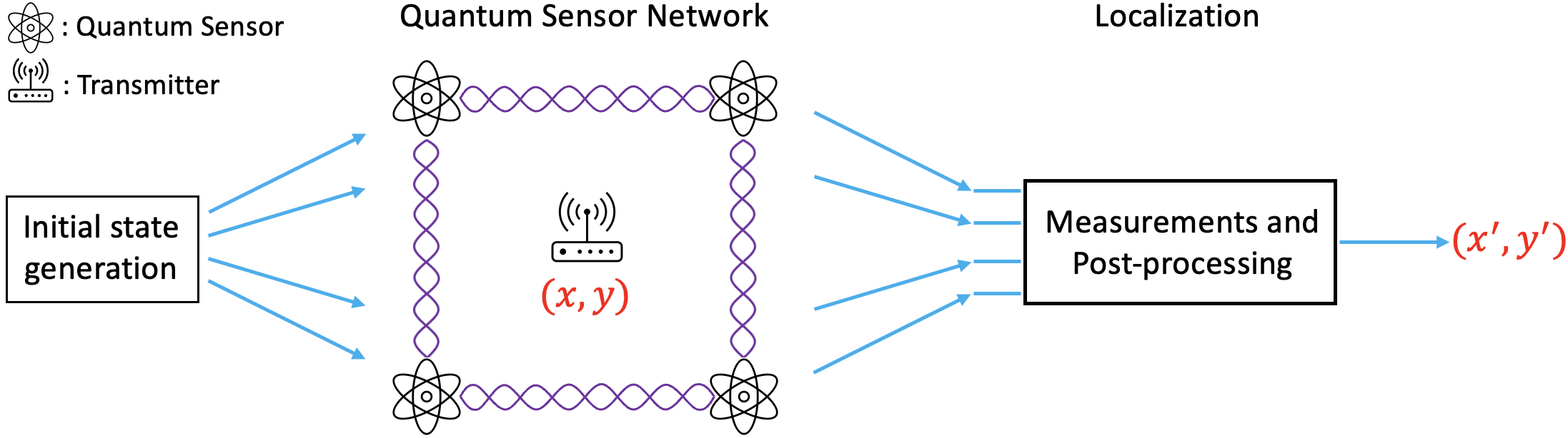
Figure 1: Overall architecture of using a QSN to localize a transmitter.

Transmitter Localization using QSNs. Our approach to transmitter localization using QSNs essentially involves posing the localization problem as a quantum state discrimination (QSD) problem [7] which is to identify the specific state a given quantum state is in (from a given set of states in which the system can be) by performing quantum measurements on the given quantum system. The overall architecture is illustrated in Fig. 1. First, a probe state is generated and distributed to the QSN. Then, once the quantum sensors have been impacted (i.e., the overall quantum state changed) due to the transmission from the transmitter’s signal, an appropriate quantum measurement is made on the quantum state of the network. The outcome of the measurement determines the quantum state, and thus, the location of the transmitter. However, the above process can be erroneous, as solving the QSD problem even optimally can incur a certain probability of (classification/discrimination) error. This paper’s goal is to develop an approach with a minimal localization error. In that context, our developed schemes in this paper are based on two ideas that extend the above basic QSD-based approach:

1. We use a two-level approach that localizes the transmitter in two stages: first, at a coarse level using a set of sensors over the entire area, and then, at a fine level within the “block” determined by the first level.

2. In addition, we circumvent the challenge of implementing a general measurement operation, by instead using a trained parameterized hybrid quantum-classical circuit that essentially implements the measurement operation and predicts the transmitter location from quantum sensor data.

Our evaluation results show that our best scheme (which combines the above two ideas) is able to achieve meter-level (1-5m) localization accuracy; in case of discrete locations, it achieves near-perfect (99-100%) classification accuracy.

Contributions. In the above context, we make the following contributions.

1. We model the transmitter localization problem as a well-studied quantum state discrimination (QSD) problem, which allows us to develop viable transmitter localization schemes using quantum sensors.

2. We design two high-level schemes to localize a transmitter in a given area deployed with a quantum sensor network. The first scheme is based on solving an appropriate quantum state discrimination problem using a global measurement, while the second scheme uses a trained hybrid quantum-classical circuit to process the quantum sensor data. Within the above high-level schemes, we also introduce a two-level localization scheme to improve the performance of the basic one-level schemes.

3. To evaluate our schemes, we model how a quantum sensor’s state evolves due to RF signals from a transmitter at a certain distance. Using this model, we evaluate our localization schemes and demonstrate their effectiveness in our custom-built simulator.

Paper Organization. The paper is organized as follows. In §II, we present our quantum sensor model, formally define the transmitter localization problem and discuss related work. In the following two sections, we describe our two classes of algorithm: quantum-state-discrimination (QSD) based scheme, and parameterized-quantum-circuit (PQC) based scheme. We discuss our evaluation results in §V, and give concluding remarks in §VI.

II Sensor Model, Problem, and Related Work

In this section, we start with motivating our choice of RF transmitter localization as an application for QSN, and then model the impact of an RF received signal on the quantum state of a quantum sensor. We then formulate the quantum localization problem and discuss related work.

Motivation for Transmitter Localization. Accurate detection and localization of a wireless transmitter (typically, using a radio-frequency (RF) wireless signal) is important in a variety of wireless and/or mobile applications, e.g., as an intruder detection in shared spectrum systems [8], localization of devices/users in indoor settings (e.g., supermarkets, museums, virtual/augmented reality applications [9]), etc. In general, transmitter localization is a key technology for location-based services, and an improvement in transmitter localization will be very beneficial to a variety of applications. In particular, in shared spectrum systems [8], there is a need to guard the shared spectrum against unauthorized usage which entails detecting and localizing unauthorized transmitters that may use and/or jam the spectrum illegally. Classical techniques for transmitter localization involve triangulation [10] or fingerprinting techniques [11] (see [12] for a survey).

Advances in quantum technologies have led to the creation of efficient quantum sensors for radio-frequency (RF) signal detection that are much more sensitive than the classical antenna-based RF sensors and are expected to cover the entire RF spectrum [13]. E.g., in [14], researchers use some distributed entangled RF-photonic quantum sensors to estimate the amplitude and phase of a radio signal, and the estimation variance beats the standard quantum limit by over 3 dB. Thus, QSNs may have a great potential in accurate localization of wireless transmitters, which is a problem of great significance in many applications.

Quantum Sensor Model. Impact on a quantum sensor due to a physical phenomenon is typically modeled by an appropriate unitary operator that results in a quantum phase change [1]. Below, we model the change in quantum phase of a sensor’s state due to an RF received signal. Since the RF received signal (and thus the change in quantum phase) depends on the sensor’s distance from the transmitter, we can use the phase change that occurs during the sensing period to localize a RF transmitter.

Sensor’s Hamiltonian. A quantum sensor’s Hamiltonian $\hat{H}(t)$ is a sum of two components [1]:

$$\hat{H}(t)=\hat{H}_{0}+\hat{H}_{V}(t)$$

where $\hat{H}_{0}$ is the internal Hamiltonian of the system and $\hat{H}_{V}(t)$ is the change in the Hamiltonian due to an external signal $V(t)$. The internal Hamiltonian $\hat{H}_{0}$ remains fixed and is equal to $E_{0}\ket{0}\bra{0}+E_{1}\ket{1}\bra{1}$, where $E_{0}$ and $E_{1}$ are energies corresponding to the $\ket{0}$ and $\ket{1}$ states respectively. The signal Hamiltonian $\hat{H}_{V}(t)$ is given by:

$$\hat{H}_{V}(t)=-\frac{1}{2}\gamma V_{\parallel}(t)\hat{\sigma}_{z}$$

where $\sigma_{z}$ is the Pauli-Z matrix, $V_{\parallel}(t)$ is parallel component of the signal $V(t)$, and $\gamma$ is the coupling of the qubit to the parallel component. In essence, the above induces a change in the spin in the $z$ axis direction resulting in a qubit phase shift. Above, ${V_{\parallel}}(t)$ at the sensor is given by:

$$V_{\parallel}(t)=E\sin(2\pi ft+\theta)$$

where $E$ is the signal’s (electric field) maximum amplitude, $f$ is the signal frequency, and $\theta$ is the signal’s phase.

Evolution Unitary Operator. Assume at time $t=0$, the quantum state is $\ket{\phi_{0}}$. Then at time $t=t^{\prime}$, the state $\ket{\phi_{t^{\prime}}}$ is,

$$\ket{\psi_{t^{\prime}}}=\hat{U}(0,t^{\prime})\ket{\psi_{0}}$$

where the time evolution unitary operator $\hat{U}(0,t^{\prime})$ due to the signal is given by:

$$\hat{U}(0,t^{\prime}) = e^{\frac{i}{\hbar}\int_{0}^{t^{\prime}}\hat{H}_{V}(t)dt}$$

$$= e^{\frac{i}{\hbar}\int_{0}^{t^{\prime}}(-\frac{1}{2}\gamma V_{\parallel}(t)\hat{\sigma}_{z})dt}$$

where $\hbar=6.626\times 10^{-34}J\cdot s$ is the plank constant. The unit of coupling $\gamma$ is $J/(V\cdot m^{-1})$, and the unit of $V_{\parallel}(t)$ is $V\cdot m^{-1}$.

Phase Shift over a Sensing Time Window. Let us represent $\hat{U}(0,t^{\prime})$ as [16, 17]

$$\hat{U}(0,t^{\prime})=e^{-\frac{i}{2}\phi\hat{\sigma}_{z}}$$ (1)

where the phase shift $\phi=\int_{0}^{t^{\prime}}\frac{\gamma}{\hbar}V_{\parallel}(t)dt$, accumulated during the sensing time $[0,t^{\prime}]$ due to the signal $V(t)$ is estimated as follows. Note that $V_{\parallel}(t)$ is a sinusoidal function—and hence, the phase shift in one full cycle ($t^{\prime}=\nicefrac{{1}}{{f}}$) is zero. To address this, we invert the qubit whenever the sinusoidal function turns from positive to negative using a $\pi$ pulse [1]. Thus, the accumulated phase in one cycle $\phi=\int_{0}^{\nicefrac{{1}}{{f}}}\frac{\gamma}{\hbar}V_{\parallel}(t)dt=\frac{2}{\pi\hbar}\gamma E\frac{1}{f}$. Since the sensing time $t^{\prime}$ is expected to be much larger than $1/f$, the phase shift accumulated during the sensing time $[0,t^{\prime}]$ can be estimated by:

$$\phi=\frac{2}{\pi\hbar}\gamma Et^{\prime}$$ (2)

Thus, for a fixed sensing time duration, the phase shift in the sensor’s quantum state accumulated due to the signal is proportional to $E$, the signal’s maximum amplitude, which is a function of the distance from the transmitter (see §V).

Impact on Multiple Quantum Sensors. Consider a set of $m$ quantum sensors distributed over an area, with a global $m$-qubit quantum state of $\ket{\psi_{0}}$. Consider a transmitter at a certain specific location in the area. Let $\hat{U}_{i}$ be the impact on the $i^{th}$ sensor due to the transmitter over a sensing time window. Then, the overall impact on the global quantum state is represented by a tensor product of $m$ individual unitary operators, i.e., $\bigotimes_{i=1}^{m}\hat{U}_{i}$, and the evolved global state state is $\bigotimes_{i=1}^{m}\hat{U}_{i}\ket{\psi_{0}}$.

Problem Definition. Consider a network of quantum sensors distributed in a geographic area and a potential transmitter/intruder in the area. Let the initial state of the system of quantum sensors network be $\ket{\psi_{0}}$. As described above, due to the transmission from the intruder, the quantum state evolves to $\ket{\psi_{t^{\prime}}}=\hat{U}\ket{\psi_{0}}$ over a period of time $t^{\prime}$. The transmitter localization problem is to determine the location of the transmitter based on the evolved quantum state $\ket{\psi_{t^{\prime}}}$.

Related Work. Radio transmitter localization using a set of sensors/receivers has been widely studied [18, 12, 19]. Localization methods can be roughly classified into two types: geometry-based and fingerprinting-based. The geometry-based method includes multilateration (by measuring time-of-flight between the transmitter and multiple sensors) or triangulation (by measuring angle-of-arrival (AoA) of the transmitter at multiple sensors) [10]. The fingerprinting-based method [11] has a training stage that records the signal fingerprint for certain locations; Localization is then achieved by matching the real-time signal to the recorded fingerprints. Here, a fingerprint for a transmitter location may be a vector of received signal strengths (RSS) [18] at the sensors. Localization of simultaneously-active multiple transmitters is more challenging, and has been addressed in recent works [20, 21, 22].

Recently, there have been some works that have used quantum technology to investigate intruder/transmitter localization related problems. E.g., [23] develops a scheme to improve the size of the fingerprints used in the above-described fingerprinting approach, by encoding classical sensor data into qubits through quantum amplitude encoding. In addition, [24] derives analytical equations to compute AoA of an incoming RF signal using four entangled distributed quantum sensors, without any evaluations. [25] proposes a quantum sensor network using Mach-Zehnder interferometers to detect (not localize) intruders for surveillance purposes. Finally, [26, 27] investigate the optimization of initial state in discrete-outcome quantum sensor networks and show that an entangled initial state yields higher measurement accuracy in some applications.

Parameter Estimation using Quantum Sensors. Prior works on parameter estimation using quantum sensors include: estimation of single [2] or multiple independent parameters [3], estimation of a single linear function over parameters [28], and estimation of multiple linear functions [29]. Our transmitter localization problem can be looked upon as a novel single parameter (TX location) estimation problem based on sensor measurements that are functions (based on signal propagation model and distance) of the parameter being estimated.

III Quantum State Discrimination Based Algorithms

Quantum State Discrimination (QSD). Given a quantum state $\ket{\phi}$ that is known to be equal to one of the states (known as target states) in the set $\{\ket{\phi_{1}},\ket{\phi_{2}},\ldots,\ket{\phi_{n}}\}$, the quantum state discrimination (QSD) problem is to determine which state $\ket{\phi}$ really is. In general, each target state $\ket{\phi_{i}}$ may be associated with a prior probability $q_{i}$; in this paper, we assume uniform prior. The QSD problem is typically solved using a series of measurements or a single measurement—as defined below. It is known that if the target states $\{\ket{\phi_{i}}\}$ are not mutually orthogonal, then there is no quantum measurement capable of perfectly (without error) distinguishing the states. Thus, a QSD solution may give an erroneous answer—i.e., guess the state to be in $\ket{\phi_{i}}$ when the state is really in $\ket{\phi_{j}}$ for some $i\neq j$. Thus, a QSD solution is associated with an overall probability of error (PoE), and the optimization goal of the QSD problem is to determine the measurement (or a sequence of measurements) that minimizes the PoE. We note that in our developed schemes, we don’t actually solve the QSD problems that arise due to the impracticality of implementing the general POVMs, as discussed later; instead, we just use the standard POVM known as pretty good measurement (PGM).

General Measurements. A general measurement [30] is defined by matrices $M_{1},M_{2},\ldots,M_{n}$ such that $\sum_{i}M_{i}^{\dagger}M_{i}=I$ where $M_{i}^{\dagger}$ is the conjugate transpose of $M_{i}$. If this general measurement is carried out on a pure state, we see the outcome “$i$” with probability $p(i)=\bra{\phi}M_{i}^{\dagger}M_{i}\ket{\phi}$. Thus, if we associate the outcome “$i$” with the given state $\ket{\phi}$ being in the target state $\ket{\phi_{i}}$, the probability of error (PoE) for the given measurement $\{M_{i}\}$ is given by $\sum_{i}\sum_{j\neq i}\bra{\phi_{i}}M_{j}^{\dagger}M_{j}\ket{\phi_{i}}$.

If we are only interested in the probability of outcomes (as in our context), the above general measurement can also be represented by the set of positive semi-definite matrices (PSD) $\{E_{i}=M_{i}^{\dagger}M_{i}\}$ where $\sum_{i}E_{i}=I$. This representation is called positive-operator valued measure (POVM); in this paper, we use this representation of measurement for simplicity.

Core Idea: TX Localization as QSD. Consider a geographic area where a transmitter can be at a set of potential locations $\{l_{1},l_{2},\ldots,l_{n}\}$. For simplicity, let us assume that the transmission power is constant. Let the initial state of the quantum system, composed of say $m$ distributed quantum sensors, be $\ket{\psi_{0}}$. When the transmitter $T$ is at a location $l_{i}$, let the impact of the $T$’s transmission from location $l_{i}$ evolve the overall state of the quantum system to $\ket{\psi_{i}}$ based on the model described in the previous section. Now, consider the set of target states $\{\ket{\psi_{1}},\ket{\psi_{2}},\ldots,\ket{\psi_{n}}\}$ corresponding to the set of potential locations of the transmitter. Then, localizing the transmitters, i.e., determining the location $l_{i}$ from where the transmission occurred, is tantamount to solving the QSD problem with the target states $\{\ket{\psi_{i}}\}$. Thus, determining the state of the quantum system yields the transmitter location.

Selection of Initial State and Measurement. In the above context, our goal is to select an initial state $\ket{\psi_{0}}$ and the POVM measurement (i.e., PSD matrices $\{E_{1},\ldots,E_{n}\}$, one for each potential outcome/location) such that the overall PoE is minimized — for a given setting of transmitter location, quantum sensors, and signal propagation model. The optimization problem of selecting an optimal combination of initial state and POVM in our context is beyond the scope of this work. Here, we use a non-entangled uniform superposition pure initial state $\ket{\psi_{0}}=\sum_{i=0}^{2^{m}-1}\frac{1}{\sqrt{2^{m}}}\ket{i}$. For a given initial state and target states, determining an optimal POVM can be shown to be a convex optimization problem and can be solved using an appropriate semi-definite program (SDP) [31]. However, due to scalability challenges in solving the SDP, whose size is exponential in the number of quantum sensors involved, in this paper, we use a well-known measurement known as pretty-good-measurement (PGM) which is known to perform well in general settings [32]. The PGM POVM is given by:

$$E_{i}=q_{i}{\rho}^{-1/2}\rho_{i}{\rho}^{-1/2}$$ (3)

where $q_{i}$ is the prior probability and $\rho_{i}=\ket{\psi_{i}}\bra{\psi_{i}}$ is the density matrix of the $i^{th}$ target state $\psi_{i}$, and $\rho=\sum_{i}q_{i}\rho_{i}$.

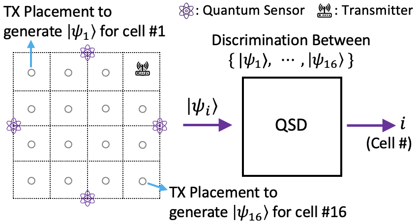
Figure 2: QSD-One Scheme.

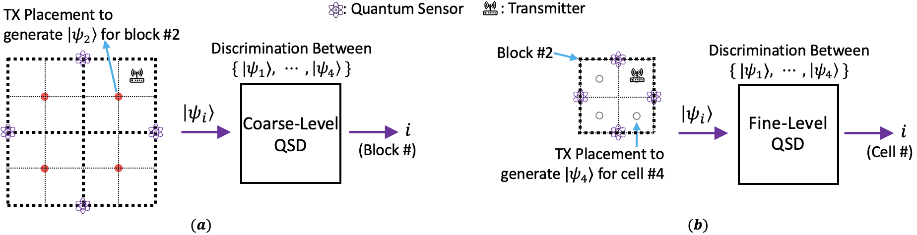
Figure 3: QSD-Two Scheme. (a) Coarse-level localization phase, and (b) Fine-level localization phase.

Basic QSD-One Scheme; Key Challenges. The above-described methodology is essentially our basic QSD-One localization scheme, see Fig. 2. That is, the QSD-One scheme localizes the transmitter by first determining the set of target states $\{\ket{\psi_{1}},\ket{\psi_{2}},\ldots,\ket{\psi_{n}}\}$ corresponding to the centers of the cells (a set of transmitter locations), and then, localizes the transmitter in real-time by performing QSD over the evolved quantum state using PGM measurement. Note that we use only the cells’ centers to generate the target states, and also that the predicted location of the transmitter is always a cell’s center in the QSD-based schemes, since the QSD-based schemes are fundamentally classification of the transmitter location into cells. However, during evaluation, the actual location of the transmitter can be anywhere in the area—presumably, non-center locations of the transmitter may incur higher localization errors.

The key challenges in the QSD-One scheme are twofold: (i) It is likely to incur a high probability of error due to a large number of target states (equal to the number of potential transmitter locations). (ii) A global POVM measurement over a large number of sensors can be difficult to implement in practice [33]; even ignoring the communication cost of teleporting the qubits to a central location, the main challenge arises due to the complexity of the circuit or hardware required to implement a POVM over a large number of qubit states. We address these challenges by designing a two-level localization scheme as described below; in the following section, we further address the above challenges by designing non-QSD based schemes.

QSD-Two Scheme. QSD-Two solves the above-mentioned challenges by localizing the transmitter by using two levels of POVMs, with each POVM requiring a measurement over a much fewer number of sensors and with a much fewer number of possible target states. We discretize the given area into a grid; each unit of the grid is called a cell. A block is a group of neighboring cells that form a rectangle. In Fig. 3 (a), a grid has $4\times 4$ cells and $2\times 2$ blocks. The thick dotted lines depict the blocks while the non-thick dotted lines depict the cells. In general, for a $N\times N$ grid with $N^{2}$ cells, we construct blocks by dividing the entire grid into $\sqrt{N}\times\sqrt{N}$ blocks — yielding $N$ blocks in the whole area, with each block comprised of $\sqrt{N}\times\sqrt{N}=N$ cells. Without loss of generality, we assume $\sqrt{N}$ to be an integer in our discussion. The basic idea of the QSD-Two scheme is to localize the transmitter in two stages: first, localize the transmitter at a block level (Fig. 3 (a)); and then, within that block, localize the transmitter at the cell level (Fig. 3 (b)). The sensors, target states, and POVMs used for localization at these two stages are different. Such a two-stage localization scheme naturally addresses the above-mentioned challenges by reducing both the number of sensors as well as target states required at each stage. We describe the scheme in more detail below.

Coarse-Level Localization. The coarse level concerns localizing the transmitter at the block level, and is done based on coarse-level sensors deployed over the entire given area. The target states for the coarse-level QSD/localization are the states corresponding to the location at the center of each block in the given area. As mentioned above, since the number of blocks is $N$, the number of target states for the Coarse-Level localization is $N$. The POVM measurement for the coarse-level localization is constructed using Eqn. 3 for the PGM measurement over the target states derived from the impact of the transmitter at coarse-level discrete locations (i.e., the center of the blocks) on the coarse-level sensors. Note that in reality, the transmitter is likely not at the center of the blocks—but, we stipulate that a block’s center is a reasonable representative of the actual locations of the transmitter in that block. More formally, let $\{L_{1},L_{2},\ldots,L_{N}\}$ denote the centers of the blocks in the area, and $S$ be the coarse-level sensors. Let $\hat{U}_{i}$ denote the impact on $S$ when the transmitter is at location $L_{i}$. Then, the target states for the coarse-level localization are $\{\hat{U}_{i}\ket{\psi_{0}}\}$ where $\ket{\psi_{0}}$ is the initial state of $S$. These target states are used to determine the POVM measurements as per Eqn. 3, and thus, determine the block.

Fine-Level Localization. Once the transmitter has been localized within a block $B$ via coarse-level localization, the transmitter is then localized at a cell level within $B$. For fine-level localization, each block $B$ has a set of fine-level sensors $S(B)$ deployed within $B$ (which need not be disjoint from the coarse-level sensors). The target states for fine-level localization within $B$ correspond to the potential locations of the transmitter within $B$ which are the centers of the cells within $B$, see Fig. 3 (b), and is derived from the impact of the transmitter’s signal at the fine-level sensors $S(B)$. Note that at the fine-level localization phase, only the sensors $S(B)$ where $B$ is the block selected in the previous coarse-level localization are involved. Note that $S(B_{1})$ and $S(B_{2})$ from two different blocks need not be disjoint. More formally, let $\{l_{1},l_{2},\ldots,l_{N}\}$ denote the centers of the cells in the block $B$ selected by the coarse-level localization phase, and $S(B)$ be the fine-level sensors. Let $\hat{U}_{i}$ denote the impact on $S(B)$ when the transmitter is at location $l_{i}$. Then, the target states for the fine level localization are $\{\hat{U}_{i}\ket{\psi_{0}}\}$ where $\ket{\psi_{0}}$ is the initial state of $S(B)$. These target states are used to determine the POVM measurement as per Eqn. 3, and thus, determine the cell within the block $B$, which is the TX location. As mentioned before in the one-level scheme, we note that, during evaluation, the location of the transmitter can be anywhere in the area, even though we have only use the cells’ centers to generate the target states.

Multi-shot Discrimination. The quantum measurement is intrinsically probabilistic and the single-shot discrimination can incur a high probability of error. One way to reduce this probability of error is to repeat the discrimination process many times and pick the most frequent measurement outcome. Such repeated measurements are commonly done in quantum sensing [1] and computing [34]. In our context, the repetitions are done while the transmitter remains fixed.

IV Parameterized Quantum Circuit Based Localization

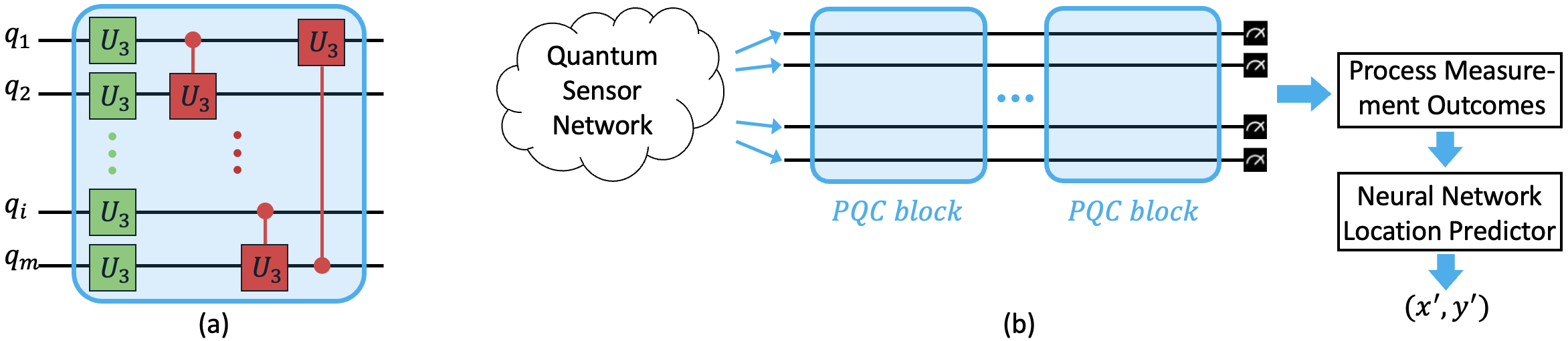
Figure 4: (a) Our parameterized quantum circuit (PQC) block, for the general case of $m$ qubits. It contains $m$ number of $U_{3}$ gates and $m$ number of $CU_{3}$ gates. (b) The hybrid quantum-classical circuit to localize a transmitter. It consists of multiple PQC blocks, followed by classical processing of measurements, and finally, a neural network-based location predictor. We use only four blocks of PQCs in our hybrid circuit.

Motivation. The QSD-based method discussed in the previous section has a solid mathematical foundation, but its practical implementation is non-trivial and even infeasible for a large sensor network and/or a large number of potential transmitter locations. In particular, the POVM measurement operator (derived from the QSD problem or corresponding to the pretty-good measurement) can be infeasible to implement for a large number of outcomes/locations. The issue is somewhat mitigated by using a two-level approach as described above, but the PoE (probability of error) in the first (coarser) level can still be high due to imperfect training (as we assign a single outcome to a set of target locations). A potential approach to address the above challenge is to “translate” a given POVM into an appropriate quantum circuit comprised of quantum gates and simple measurements (e.g., projective and/or computational basis) [33]. E.g., [35] presents a technique to convert POVM operators to such quantum circuits. However, the computational time incurred in translating a POVM operator into a quantum circuit is exponential to the number of qubits and is thus infeasible. In addition, the translated quantum circuits are also sub-optimal in terms of the number of CNOT gates used [35]. Also, note that the POVM computed in our QSD-based method is sub-optimal to begin with.

In this section, we develop a machine learning (ML) technique to actually learn a quantum circuit that represents the processing and measurement protocol needed to localize the transmitter from the evolved quantum state. The learned quantum circuit model maps the global evolved quantum state to the transmitter location. In essence, we avoid computing the POVM (from QSD, or using the pretty-good measurement) altogether (and thus, also avoid the challenge of translating it to a quantum circuit), and instead learn the required quantum circuit representing the measurement protocol. To facilitate learning the quantum circuit, we use an appropriate parameterized quantum circuit (PQC) and learn its parameters—as in [36] wherein a POVM is trained using parameterized quantum circuits. Our PQC-based localization method based on the above insights is described below. We start with a brief introduction to PQCs.

Parameterized Quantum Circuits (PQC). Parameterized quantum circuits have emerged as a powerful tool in quantum computing [37], providing an adaptable framework for tackling diverse computational tasks. Parameterized quantum circuits (PQCs) can be regarded as machine learning models with remarkable expressive power; just like classical ML models, PQC circuits/models are trained to perform data-driven tasks. PQCs offer several advantages over fixed quantum circuits [37, 38, 39], including:

1. Adaptability. The parameters in PQCs can be adjusted to tailor the circuit for a specific problem, allowing a single circuit structure to be repurposed for various tasks.

2. Trainability. PQCs can be trained using classical optimization algorithms to solve optimization problems and machine learning tasks, making them a vital component of hybrid quantum-classical algorithms.

3. Noise Resilience. PQCs can be more robust against noise and errors in near-term quantum devices, as they allow shorter-depth circuits that reduce the impact of errors.

In essence, PQCs are quantum circuits comprised of parameterized gates and measurements. Commonly used parameterized gates in PQCs include rotation gates $R_{x}(\theta),R_{y}(\theta),R_{z}(\theta)$ which represents rotating about the $X,Y,Z$ axis respectively with angle $\theta$. A more versatile gate is the $U_{3}(\theta,\phi,\lambda)$, which can be used to generate any single-qubit operation by setting the appropriate values for the parameters; $U_{3}$ gate can be decomposed into simpler $R_{x},R_{y},R_{z}$ gates. The parameterized $CU_{3}(\theta,\phi,\lambda)$ gate is the controlled version of the $U_{3}$ gate; it applies the $U_{3}$ gate only when the control qubit is in the $\ket{1}$ state. We use a combination of $U_{3}$ and $CU_{3}$ gates in our parameterized quantum circuits.

PQC-based Localization Method. At a high level, in our PQC-based localization scheme, the QSN data is fed into a trained hybrid quantum-classical model, which represents the overall measurement strategy and thus outputs the transmitter location. Our hybrid quantum-classical model (see Fig. 4(b)) consists of the following three components. (i) Parameterized Quantum Circuit (PQC), (ii) Processing the measurement outcomes, (iii) Neural network location predictor, to convert the processed measurement outcomes to the transmitter location. We describe each of the above components below.

1. Parameterized Quantum Circuit (PQC) Design. The parameterized quantum circuit can be designed in many ways. We design our PQC component based on some common PQC-design patterns [40, 41] used in prior works. For example, in [42], a block of PQC contains one layer of $ZZ$ gates and one layer of $R_{y}$ gates. In [43], a block of PQC contains one layer each of $R_{x},R_{y},R_{z},CZ$ gates. In our scheme, the quantum circuit is composed of blocks, and each block is a combination of $U_{3},CU_{3}$ gates; we use these two gates in our design as they form a universal gate set and are widely used in PQC circuits. Circuits consisting $U_{3}$ and $CU_{3}$ gates have a high expressive power as each gate has three trainable parameters. In particular, given $N$ number of input qubits, a block consists of $N$ number of $U_{3}$ and $N$ number of $CU_{3}$ gates. See Fig. 4. In a block, each input qubit is first operated on by the unary $U_{3}$ gate in parallel, forming a layer of $U_{3}$ gates. Then, there is a series of $CU_{3}$ gates following a ring connection pattern, i.e., each $CU_{3}$ is executed over two “consecutive” qubits (with the first being the control qubit) except for the last $CU_{3}$ gate which is over the last and the first qubit. Thus, a single block has a circuit depth of $N+1$. The overall PQC may have a series of above blocks—the expressive power of the model increases monotonically with the increase in the number of blocks. In our evaluations (§V), we used four blocks as we observe that four blocks provide good performance while having a modest circuit depth. After the blocks, the PQC ends with the measurement on the standard computational basis, i.e., the Pauli Z basis.

2. Process Measurement Outcomes. As in the QSD-based schemes, we will use the PQC to make repeated measurements. To use the repeated measurements effectively for location prediction, we characterize the set of repeated measurement results by expectation values, one for each qubit. In particular, we compute the expectation value $\langle Z\rangle$ of the Pauli Z operator (which represents the measurement in the computational basis), and feed as input to a neural network for final location prediction as described below. We note that, for a quantum state $\ket{\psi}=\alpha\ket{0}+\beta\ket{1}$, the expectation value $\langle Z\rangle$ of the Pauli Z operator is given by $\bra{\psi}Z\ket{\psi}=|\alpha|^{2}-|\beta|^{2}$.

3. Neural-Network to Predict Location. We consider two variants of our neural network predictor: (i) Classifier variant. which outputs a class/label corresponding to the cell where the TX is located, and thus, predicts the location to be the cell’s center. (ii) Regression variant, that outputs locations as the $x$ and $y$ coordinates.

Classifier Variant. Our overall circuit with the Classifier component for the location prediction essentially equates to a circuit for quantum state discrimination (QSD), as the QSD problem also outputs a finite number of discrete outcomes. For the Classifier Variant, we use a simple neural network with only an input layer and an output later, having no hidden layers—i.e., a single fully connected layer. The input neurons are the expectation values of the Pauli Z operator from the measurements as described above, and the output neurons represent the cell labels. See Fig.5(a), which shows the fully connected layer for a network of 4 quantum sensors deployed in a $4\times 4$ grid with 16 cells.

Regression Variant. The Classifier Variant outputs locations in a discrete space—which is fundamentally sub-optimal if the transmitter can be anywhere in the 2D space. To output the predicted location in the continuous 2D space, we use a Regression Variant that outputs the location as an $(x,y)$ point. For the setting wherein the transmitter may be located anywhere in the 2D space, the Regression Variant should have a smaller localization error. Fig.5(b) shows the fully connected layer for the Regression Variant; the number of output neurons is always two, i.e., a $X$ coordinate and a $Y$ coordinate.

4. Loss Function. During training, the gradient of the loss function is back-propagated through the neural network and the quantum circuit parts, so that the parameters within these parts can be appropriately updated. The loss functions used for the Classifier Variant and the Regression Variant are different; for the Classifier variant, we use the cross-entropy loss function while for the Regression variant, we use the mean square error loss function.

PQC-One and PQC-Two Schemes. The above-described hybrid quantum-classical model is essentially our PQC-One localization scheme. By using PQC-One as a building block and using the same two-level (coarse, fine) idea described in §III, we design the PQC-Two, corresponding to the two-level QSD-based schemes described in the previous section. At the first coarse level, the output of the “coarse-level PQC-One” will determine the block the transmitter is in. Then at the second fine level, the output of the “fine-level PQC-One” tied to the block determined by the coarse level is the final location output. The PQC-based schemes essentially use the trained circuit in lieu of the POVM used in the QSD-based schemes. The PQC-based schemes can be used with either the Classifier or the Regression variant for the last predictor component.

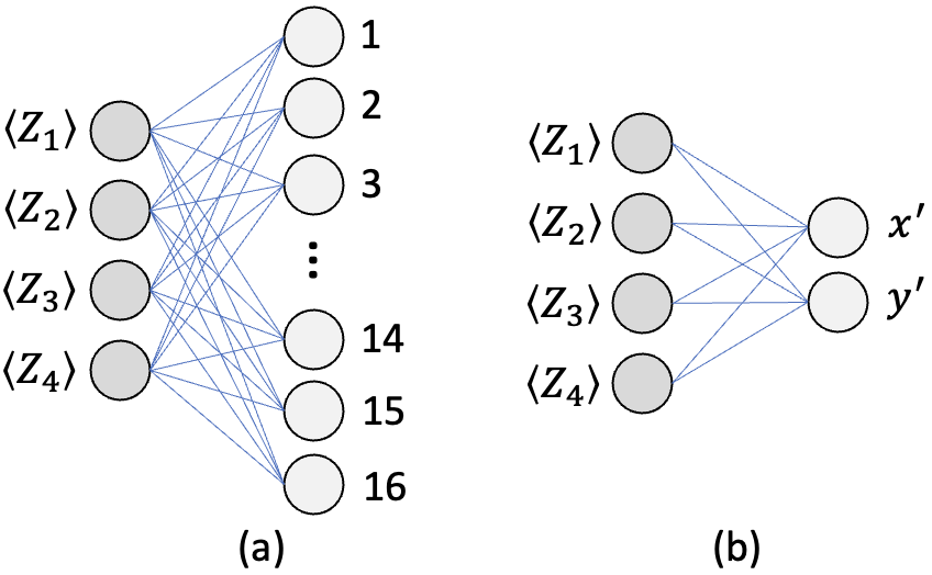
Figure 5: Neural network (a fully connected layer) for 4 quantum sensors to predict the location from processed measurements. (a) Classifier Variant, (b) Regression Variant.

V Evaluation

In this section, we evaluate our developed schemes. We make two observations, which are as expected: (1) Performance of two-level methods is better than one-level methods in general, and (2) Performance of the PQC-based methods is superior to the QSD-based methods. In summary, our schemes are able to achieve meter-level (1-5m) localization accuracy, and near-perfect (99-100%) classification accuracy in the case of discrete locations.

V-A Evaluation Settings

Algorithms Evaluated. We evaluate four algorithms: QSD-One, QSD-Two, PQC-One, PQC-Two. As the name implies, QSD-One and PQC-One are one-level methods, while QSD-Two and PQC-Two are two-level methods. Similarly, QSD-One and QSD-Two are QSD-based methods, while PQC-One and PQC-Two are PQC-based methods. We use the Regression Variant in our PQC-based methods by default, since in our default setting the transmitter can be anywhere in the 2D space. Our code is written in Python and uses Numpy and Scipy libraries to perform matrix-related operations.

QSD-based Method Implementation. To implement the QSD-based methods, we first determine the target states which are then used to construct the pretty-good-measurement POVM via Eqn. 3. To localize a transmitter, we first compute the evolved state and then, use the POVM to determine the target state or the TX location. This is done repeatedly as described in Section III, and in two levels (coarse, fine) depending on the localization scheme. The target states and evolved states are both generated using the sensor model described in Section II, i.e., using Eqns. 1-2, with the electric field strength ($E$) and phase shift range modeled as below.

Generating Sensor Readings. The crux of determining target states, computing the evolved states, and simulating the training datasets is to compute the phase shift picked up by the quantum sensors due to the signal during the sensing process. In Eqn. 2, we modeled the phase shift as a function of the electric field strength and the sensing time. Thus, we need a model for the electric field strength. In free space, the electric field strength produced by a transmitter with an isotropic radiator can be approximated as [44]

$$E=\frac{\sqrt{30\cdot P}}{d}\times(1+noise)$$

where $E$ is the electric field strength in $V\cdot m^{-1}$, $P$ is the transmitter power output in $W$ (watt), and $d$ is the distance from the radiator in $m$. Since in most quantum sensing applications, the signal to be sensed are weak signals, here we assume the power of the transmitter $P=0.1\mu W$. Ideally, the strength of the electric field is inverse to the distance between the transmitter and the sensor. But in reality, the relationship is more complicated. So, we add a random uniform variable $noise\in[-0.05,0.05]$ to incorporate reality in a simple way. The target states and thus the POVMs are computed assuming zero noise during training, while during localization, the signal received is assumed to contain noise. The simulated datasets for PQC-based methods are assumed to contain noise too.

Range of Phase Shift $\phi$. We set the sensing time $t^{\prime}$ to 1 millisecond. As mentioned later, our grid cells are $10m\times 10m$, and we assume 5 meters to be the minimum distance allowed between a transmitter and a quantum sensor. Thus, we choose the coupling constant $\gamma$ to be such that a quantum sensor at 5 meters away from the transmitter accumulates a phase shift of $2\pi$ during the sensing time $t^{\prime}$; this entails that the maximum phase shift is $2\pi$ and the minimum phase shift is as low as $0$ (when the sensor is very far away from the transmitter).

PQC-Based Methods Implementation and Training. Different than the QSD-based methods, the PQC-Based methods involve quantum circuits. We use the publicly available TorchQuantum [38] library to implement and train the parameterized hybrid circuits. TorchQuantum’s classes are inherited from a core class of PyTorch [45], which is used to implement the neural network predictor. Thanks to PyTorch, we are able to train the PQCs fast on a GPU. We use the Adam optimizer and train for 80 epochs for both PQC-One and PQC-Two methods.

The sensor readings are also used as the sensor data to train the PQC-based hybrid circuit models. Essentially, for a fixed initial global state of the sensors (say, $\psi$), each sample consists of the quantum state received from the quantum sensor network (input feature) and the location of the transmitter (ground truth target). More formally, each sample is of the kind: $(\bigotimes_{i=1}^{m}\hat{U}_{i}\ket{\psi},L)$, where $\hat{U}_{i}$ is the evolution unitary operator for the $i^{th}$ quantum sensor (as per §II and above paragraphs), $\ket{\psi}$ is the uniform superposition initial state, and $L$ is the location of the transmitter in the field in all scenarios except for one, i.e., $L$ is the block number for samples used to train a “coarse-level PQC-One” in the PQC-Two Classifier Variant. We use one hundred training examples/samples for each cell, with the transmitter’s location randomly scattered over the cell. For example, consider a $4\times 4$ grid with a block length of 2. The training dataset for PQC-One will have $16\times 100=1600$ samples. And PQC-Two will have $16\times 100=1600$ samples in the first level to train a “coarse-level PQC-One”, and $4\times 400=1600$ samples in the second level to train 4 blocks each requiring $4\times 100=400$ to train a “fine-level PQC-One”. Thus, there are a total of 3600 training samples used to train 5 models in a PQC-Two method.

Quantum Sensor Deployment. We deploy sensors uniformly over the area; for the QSD-Two and PQC-Two schemes, we deploy the fine-level sensors along the block borders so that the sensors can be used by the two neighbor blocks, i.e. fine-level sensors for the blocks are not disjoint. We use a maximum of 8 quantum sensors for any single QSD instance—since the memory and computing requirements for storing and implementing a POVM become prohibitive beyond that. E.g., a POVM for 256 target-states over 12 sensors requires 69 GB of main memory storage. The PQC-based methods have a bottleneck on the number of sensors due to POVM considerations, but we are still limited in practice nevertheless due to training time and GPU memory; thus, we use a maximum of 16 sensors in the first level or in any block of the second level. This limits the training time to at most several hours and GPU memory requirements to 8-16 GB. We discuss more details on number of sensors used at various levels and blocks, below. Finally, each grid cell is of size $10m\times 10m$ in all settings, and the transmitter can be anywhere in the given area except that the minimum distance between any sensor and transmitter is 5m.

Two-Level Schemes: Blocks and Sensors Used. As described in §III, for a grid $N\times N$, if $N$ as a perfect square, the grid is divided into $\sqrt{N}\times\sqrt{N}$ blocks—with the first-level localizing the transmitter into one of the blocks, and the second-level localizing the transmitter into a cell within the block. However, in this section, to get a better insight into the performance trends, in this section, we have also considered $N$ values that are not perfect squares. For such $N$ values, we have determined block sizes as integers close to the $\sqrt{N}$; e.g., for a $12\times 12$ grid, we divided the grid into $4\times 4$ blocks each of $3\times 3$ cells. In terms of the number of sensors at each level—we use up to 16 sensors in the first-level of localization, but in the second-level we always use exactly 4 sensors per block irrespective of the block/grid size.

Performance Metrics. We use the Localization error ($\mathrm{L_{err}}$, in meters) as the main metric to evaluate our localization schemes. $\mathrm{L_{err}}$ is defined as the distance between the actual location of the transmitter and the predicated location. In all plots except the CDF plots, average $\mathrm{L_{err}}$ refers to the average localization error over many TX locations; in the CDF plots, the distribution is over many TX locations.

V-B Evaluation Results

In our evaluation, we evaluate the performance of our proposed four localization algorithms’ performances for varying grid size and number of quantum sensors. Note that, for one-level algorithms, the number of sensors is the total number of sensors used, while for the two-level algorithms, the number of sensors parameter is the number of sensors used in the first/coarse level (recall that, in the second level, we use only 4 sensors for each block).

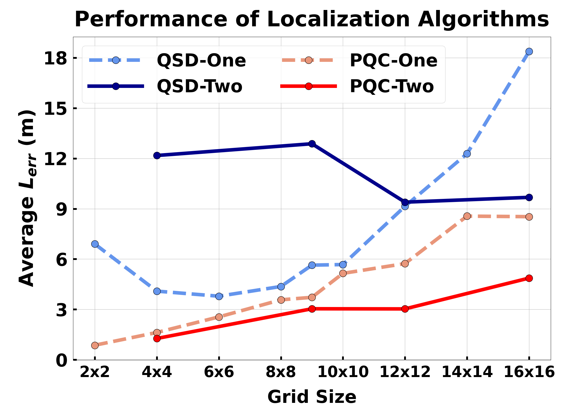
Figure 6: The performance of QSD-One, QSD-Two, PQC-One, PQC-Two for varying grid size and 8 quantum sensors.

Varying Grid Size. Fig. 6 shows the performance of all four algorithms with varying grid sizes when the number of quantum sensors is eight. We observe that the PQC-based methods have lower localization error than the QSD-based methods, and the two-level schemes generally perform better than one-schemes—except that the QSD-Two performs worse than QSD-One for smaller grid sizes. The results show the power of a well-trained parameterized hybrid circuit and the effectiveness of two-level schemes. More specifically, we observe that for a $16\times 16$ grid, the average $\mathrm{L_{err}}$ of PQC-Two is $4.9m$, which is almost half of the average $\mathrm{L_{err}}$ of PQC-One at $8.5m$. Similarly, the $\mathrm{L_{err}}$ of QSD-Two is also almost half of the $\mathrm{L_{err}}$ of QSD-One, i.e., $9.6m$ vs $18.3m$.

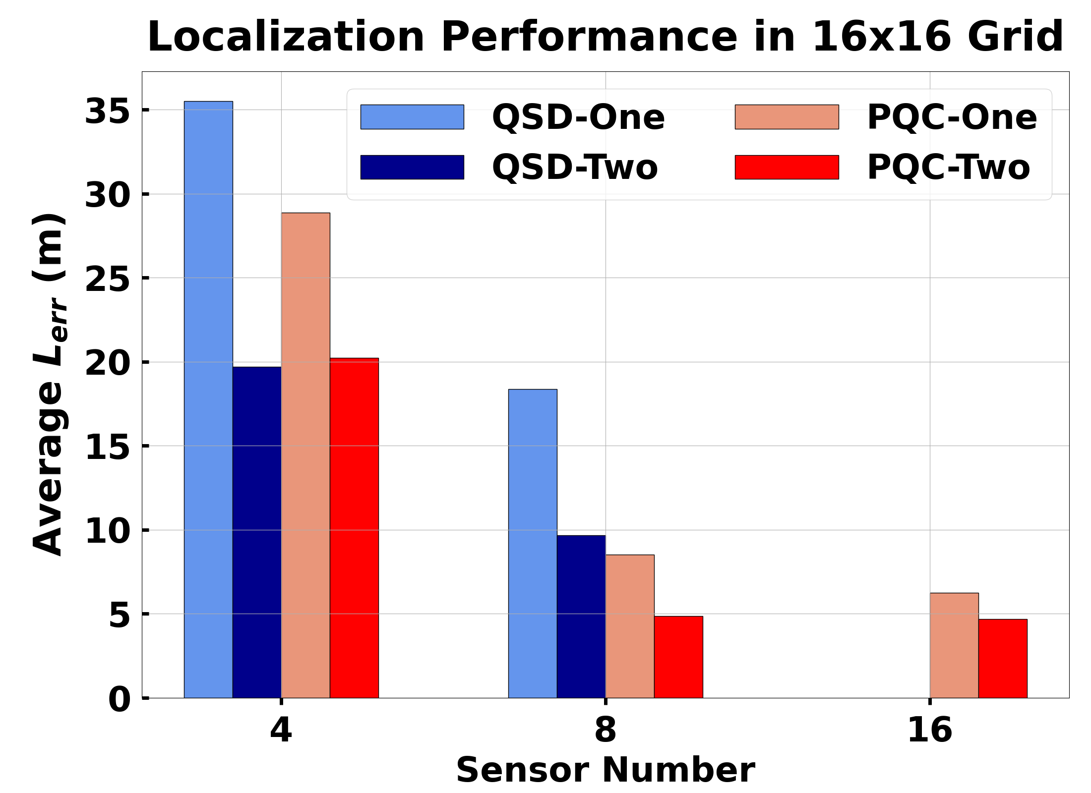
Figure 7: The performance of QSD-One, QSD-Two, PQC-One, PQC-Two for varying sensor number and a $16\times 16$ grid.

Varying Number of Sensors. Fig. 7 shows the average $\mathrm{L_{err}}$ in a $16\times 16$ grid with a varying number of quantum sensors. As expected, we observe that the $\mathrm{L_{err}}$ improves with an increasing number of quantum sensors, for all four schemes. For the PQC-Two scheme, we observe that the $\mathrm{L_{err}}$ improvement from 8 sensors to 16 sensors is minimal, i.e. $4.9m$ vs $4.7m$. This is because having 8 sensors in the first/coarse level seems sufficient to determine the block, and then, in the second level, each block will always have 4 sensors associated with it (performance in the fine level is the same).

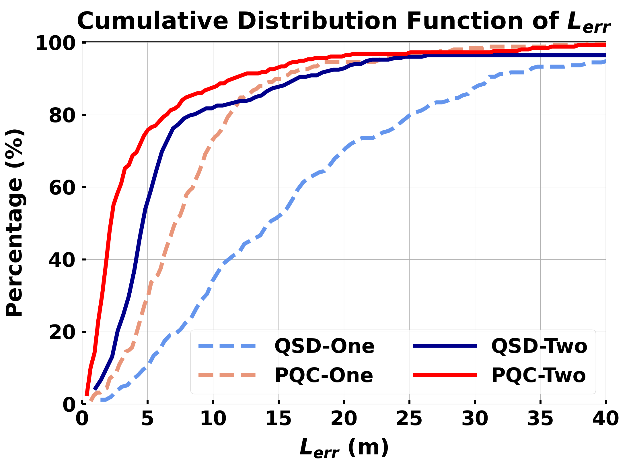
Figure 8: The cumulative probability of $\mathrm{L_{err}}$ of QSD-One, QSD-Two, PQC-One, PQC-Two for a $16\times 16$ grid and 8 quantum sensors.

CDF. Fig. 8 shows the cumulative distribution function of $\mathrm{L_{err}}$ for four methods when the grid size is $16\times 16$ and the number of sensors is 8. This plot gives insight into the distribution of $\mathrm{L_{err}}$ over different TX location, compared with Fig. 7 which shows only average $\mathrm{L_{err}}$ across many TX locations. Here, the distribution is over 256 TX locations—one random TX location per cell for 256 cells in the $16\times 16$ grid. We observe, as expected, that the two-level schemes are better than the one-level schemes, and the PQC-based methods are better than the QSD-based methods, except that QSD-Two has a better CDF plot than PQC-One up to the 83-th percentile. The above exception implies that QSD-Two has higher number of locations with large $\mathrm{L_{err}}$ compared with PQC-One; this is likely due to QSD-Two incurring errors in determining the block at the first/coarse level, which can lead to large localization errors.

Discrete Setting: In the previous evaluation results, we have considered the practical continuous setting wherein the transmitter can be anywhere in the area. To evaluate the true performance of our QSD-based methods, which are fundamentally classification strategies, we now evaluate the discrete setting wherein the transmitter is located only at the center of a cell and the predicted output of a localization method is the cell number of the transmitter. In this discrete setting, we evaluate the performance metric of Classification Accuracy $\mathrm{CC_{acc}}$ which is the percentage of times the method is correct in predicting the cell number. Also, in this discrete setting, the PQC-based methods use the Classification variant in the location predictor component, while the QSD-based methods remain the same.

Fig. 9 shows the performance of the four algorithms with varying grid sizes when the number of quantum sensors is eight. We observe similar trend for each algorithm as well as similar relative trends among the algorithms as in the continuous setting. We make two important observations:

1. First, in the QSD-based methods, the QSD-Two is a significant improvement over QSD-One (from 13% to 77% for grid side $16\times 16$), which shows the effectiveness of our two-level approach.

2. Second, for the largest grid size of $16\times 16$, the $\mathrm{CC_{acc}}$ for QSD-based QSD-Two is reasonable at 77% but is further improved impressively by PQC-Two at 97%; this shows the effectiveness of our PQC-based methods. The 3% error here in PQC-Two is mainly due to the errors in the first level of determining the block.

Also, we see that for lower grid sides, the QSD-Two surprisingly performs worse than QSD-One; the reason for this is similar to the continuous case that determining the blocks at the first level becomes more erroneous when the grid size is small.

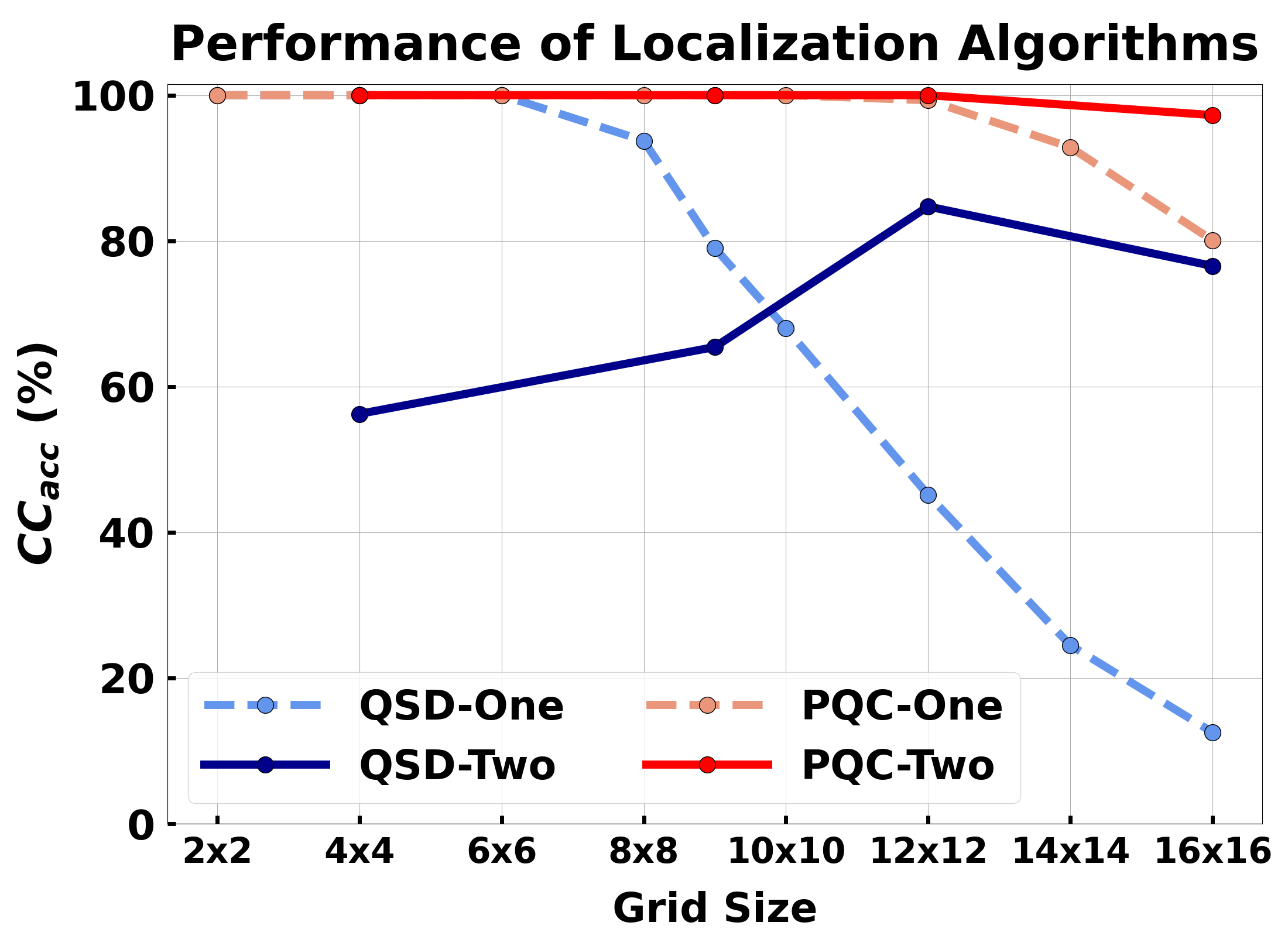
Figure 9: Performance of QSD-One, QSD-Two, PQC-One, PQC-Two for varying grid size and 8 sensors.

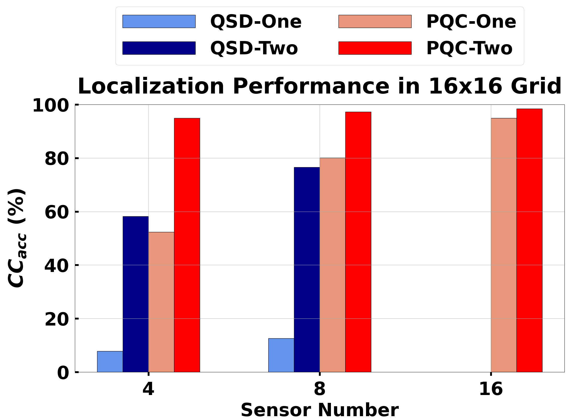
Figure 10: Performance of QSD-One, QSD-Two, PQC-One, PQC-Two for varying sensor number and a $16\times 16$ grid.

Fig.10 shows the $\mathrm{CC_{acc}}$ in a $16\times 16$ grid for varying number of quantum sensors. As expected, we observe that the $\mathrm{CC_{acc}}$ improves with an increasing number of quantum sensors. More importantly, the $\mathrm{CC_{acc}}$ for PQC-Two is near-perfect at $99\%$ with 16 sensors; this shows the effectiveness of the two-level method as well as of the well-trained parameterized hybrid circuits. As in the continuous-domain setting, we don’t show the QSD-methods for 16 sensors, as it was infeasible to implement the QSD-based methods for a large number of sensors.

VI Conclusion and Future Work

In this paper, we have developed effective schemes for an important quantum sensor network application, viz., localization of a wireless transmitter. The work demonstrates how a network of quantum sensors can collaborate to predict a parameter (here, location of an event/transmitter) that is received/sensed differently at different sensor locations (e.g., depending on the distance from the event). In particular, this work shows the promise of quantum sensor networks in localization of events in general—one of the most important applications of classical sensor networks.

Our work has significant opportunities for improvement. In particular, one can optimize the initial state of the sensors to further improve the localization performance (note that, here, we have only used a uniform superposition initial state). In this context, we are also interested in determining whether entangled initial states are helpful; recent works [46, 47, 48] have shown that entangled states can be efficiently distributed over a quantum network. In addition, one can consider general multi-level approaches and restricted forms of measurement, design parameterized quantum circuits with noise [38], and develop techniques to distribute such circuits over a quantum (sensor) network as in [49, 50, 51]. We plan to explore some of these directions in our future work.

References

- [1] C. L. Degen, F. Reinhard, and P. Cappellaro, “Quantum sensing,” Rev. Mod. Phys., vol. 89, p. 035002, 2017.
- [2] V. Giovannetti, S. Lloyd, and L. Maccone, “Advances in quantum metrology,” Nature Photonics, 2011.
- [3] T. J. Proctor, P. A. Knott et al., “Multiparameter estimation in networked quantum sensors,” Physical Review Letters, 2018.
- [4] K. S. Adu-Manu, C. Tapparello, W. Heinzelman et al., “Water quality monitoring using wireless sensor networks: Current trends and future research directions,” ACM Trans. on Sensor Networks, 2017.
- [5] O. Chipara, C. Lu, T. C. Bailey, and G.-C. Roman, “Reliable clinical monitoring using wireless sensor networks: Experiences in a step-down hospital unit,” in SenSys, 2010.
- [6] T. He, C. Huang, B. M. Blum, J. A. Stankovic, and T. Abdelzaher, “Range-free localization schemes for large scale sensor networks,” in MobiCom, 2003.
- [7] J. Bergou, “Quantum state discrimination and selected applications,” Journal of Physics: Conference Series, Oct 2007.
- [8] A. Chakraborty, A. Bhattacharya et al., “Spectrum patrolling with crowdsourced spectrum sensors,” in IEEE INFOCOM, 2018.
- [9] H. Gupta, M. Curran, J. Longtin et al., “Cyclops: An fso-based wireless link for vr headsets,” in SIGCOMM, 2022.
- [10] J. Xiong and K. Jamieson, “ArrayTrack: A Fine-Grained indoor location system,” in NSDI. USENIX Association, 2013.
- [11] P. Bahl and V. N. Padmanabhan, “RADAR: An in-building RF-based user location and tracking system,” in IEEE INFOCOM, 2000.
- [12] L. Cheng, C. Wu, Y. Zhang, C. Maple et al., “A survey of localization in wireless sensor network,” IJDSN, 2012.
- [13] D. H. Meyer, P. D. Kunz, and K. C. Cox, “Waveguide-coupled rydberg spectrum analyzer from 0 to 20 ghz,” Phys. Rev. Applied, 2021. [Online]. Available: https://link.aps.org/doi/10.1103/PhysRevApplied.15.014053
- [14] Y. Xia, W. Li et al., “Demonstration of a reconfigurable entangled radio-frequency photonic sensor network,” Phys. Rev. Lett., 2020.
- [15] C. Egerstrom, “A mathematical introduction to quantum sensing,” 2023, https://cklixx.people.wm.edu/teaching/math300/ChrisE.pdf.
- [16] L. Liu, Y. Zhang, Z. Li et al., “Distributed quantum phase estimation with entangled photons,” Nature Photonics, 2021.
- [17] Z. Zhang and Q. Zhuang, “Distributed quantum sensing,” Quantum Science and Technology, vol. 6, no. 4, p. 043001, 2021.
- [18] T. Yu, A. Haniz, K. Sano et al., “A guide of fingerprint based radio emitter localization using multiple sensors,” IEICE Trans. on Communications, 2018.
- [19] M. Ghaderibaneh, M. Dasari, and H. Gupta, “Multiple transmitter localization under time-skewed observations,” in 2019 IEEE International Symposium on Dynamic Spectrum Access Networks (DySPAN), 2019.
- [20] C. Zhan, M. Ghaderibaneh, P. Sahu, and H. Gupta, “DeepMTL: Deep learning based multiple transmitter localization,” in IEEE WoWMoM, 2021, pp. 41–50.
- [21] C. Zhan, H. Gupta, A. Bhattacharya, and M. Ghaderibaneh, “Efficient localization of multiple intruders for shared spectrum system,” in ACM/IEEE IPSN, 2020.
- [22] C. Zhan, M. Ghaderibaneh, P. Sahu, and H. Gupta, “Deepmtl pro: Deep learning based multiple transmitter localization and power estimation,” Pervasive and Mobile Computing, vol. 82, p. 101582, 2022.
- [23] A. Shokry and M. Youssef, “A quantum algorithm for rf-based fingerprinting localization systems,” in IEEE LCN, 2022.
- [24] X. Sun, W. Li, Y. Tian, F. Li, L. Tian, Y. Wang, and Y. Zheng, “Quantum positioning and ranging via a distributed sensor network,” Photonics Research, Dec 2022.
- [25] M. Nagy and N. Nagy, “Intrusion detection quantum sensor networks,” Sensors, 2022.
- [26] M. Hillery, H. Gupta, and C. Zhan, “Discrete outcome quantum sensor networks,” Physical Review A, 2023.
- [27] C. Zhan, H. Gupta, and M. Hillery, “Optimizing initial state of detector sensors in quantum sensor networks,” 2023, arXiv, 2306.17401.
- [28] S. Altenburg and S. Wölk, “Multi-parameter estimation: global, local and sequential strategies,” Physica Scripta, 2018.
- [29] J. Rubio et al., “Quantum sensing networks for the estimation of linear functions,” Journal of Physics A: Mathematical and Theoretical, 2020.
- [30] M. A. Nielsen and I. L. Chuang, Quantum Computation and Quantum Information, 10th ed. Cambridge University Press, 2011.
- [31] Y. C. Eldar, A. Megretski et al., “Designing optimal quantum detectors via semidefinite programming,” IEEE Trans. Information Theory, 2003.
- [32] P. Hausladen and W. K. Wootters, “A ‘pretty good’ measurement for distinguishing quantum states,” Journal of Modern Optics, 1994.
- [33] Y. Yordanov and C. Barnes, “Implementation of a general single-qubit positive operator-valued measure on a circuit-based quantum computer,” Physical Review A, 2019.
- [34] P. W. Shor, “Polynomial-time algorithms for prime factorization and discrete logarithms on a quantum computer,” SICOMP, 1997.
- [35] R. Iten, O. Reardon-Smith, E. Malvetti, L. Mondada, G. Pauvert, E. Redmond, R. S. Kohli, and R. Colbeck, “Introduction to universalqcompiler,” 2021.
- [36] A. Patterson, H. Chen, L. Wossnig, S. Severini, D. Browne, and I. Rungger, “Quantum state discrimination using noisy quantum neural networks,” Phys. Rev. Res., 2021.
- [37] M. Benedetti, E. Lloyd, S. Sack, and M. Fiorentini, “Parameterized quantum circuits as machine learning models,” Quantum Science and Technology, nov 2019. [Online]. Available: https://dx.doi.org/10.1088/2058-9565/ab4eb5
- [38] H. Wang, Y. Ding, J. Gu, Z. Li, Y. Lin, D. Z. Pan, F. T. Chong, and S. Han, “Quantumnas: Noise-adaptive search for robust quantum circuits,” in HPCA, 2022.
- [39] H. Wang, J. Gu, Y. Ding, Z. Li, F. T. Chong et al., “Quantumnat: Quantum noise-aware training with noise injection, quantization and normalization,” in DAC, 2022.
- [40] Z. Liang, J. Cheng, R. Yang, H. Ren, Z. Song, D. Wu, X. Qian, T. Li, and Y. Shi, “Unleashing the potential of llms for quantum computing: A study in quantum architecture design,” 2023.
- [41] Z. Wang, Z. Liang, S. Zhou, C. Ding, Y. Shi, and W. Jiang, “Exploration of quantum neural architecture by mixing quantum neuron designs,” in IEEE/ACM International Conference On Computer Aided Design (ICCAD), 2021, pp. 1–7.
- [42] S. Lloyd, M. Schuld, A. Ijaz, J. Izaac, and N. Killoran, “Quantum embeddings for machine learning,” 2020.
- [43] J. R. McClean, S. Boixo, V. N. Smelyanskiy, R. Babbush, and H. Neven, “Barren plateaus in quantum neural network training landscapes,” Nature Communications, 2018.
- [44] Wikipedia, “Field strength meter,” 2023, https://en.wikipedia.org/wiki/Field_strength_meter.
- [45] A. Paszke, S. Gross, F. Massa, A. Lerer et al., “Pytorch: An imperative style, high-performance deep learning library,” in Advances in Neural Information Processing Systems 32. Curran Associates, Inc., 2019.
- [46] M. Ghaderibaneh, C. Zhan, H. Gupta, and C. R. Ramakrishnan, “Efficient quantum network communication using optimized entanglement swapping trees,” IEEE Transactions on Quantum Engineering, vol. 3, pp. 1–20, 2022.
- [47] M. Ghaderibaneh, H. Gupta, C. Ramakrishnan et al., “Pre-distribution of entanglements in quantum networks,” in IEEE International Conference on Quantum Computing and Engineering (QCE), 2022.
- [48] M. Ghaderibaneh, H. Gupta, and C. Ramakrishnan, “Generation and distribution of GHZ states in quantum networks,” in IEEE International Conference on Quantum Computing and Engineering (QCE), 2023.
- [49] R. G Sundaram, H. Gupta, and C. Ramakrishnan, “Efficient distribution of quantum circuits,” in 35th International Symposium on Distributed Computing, 2021.
- [50] R. G. Sundaram, H. Gupta, and C. Ramakrishnan, “Distribution of quantum circuits over general quantum networks,” in IEEE International Conference on Quantum Computing and Engineering (QCE), 2022.
- [51] R. G. Sundaram and H. Gupta, “Distribution of quantum circuits using teleportations,” in IEEE International Conference on Quantum Software (QSW), 2023.