STREAMING TARGET SOUND EXTRACTION USING ATTENTION QUERIES

Causal TARGET SOUND Selection USING ATTENTION QUERIES

Transformers for causal label-based source extraction

Real-time TARGET SOUND EXTRACTION USING ATTENTION QUERIES

Causal Target source extraction using a transformer decoder

Real-time label-based sound extraction

Real-time TARGET SOUND EXTRACTION USING Transformers

Streaming TARGET SOUND EXTRACTION using attention

Real-time TARGET SOUND EXTRACTION using attention

Real-time TARGET SOUND EXTRACTION

Waveformer: Transformer for Real-time TARGET SOUND EXTRACTION

Real-time TARGET SOUND EXTRACTION

Real-time TARGET SOUND EXTRACTION

Abstract

We present the first neural network model to achieve real-time and streaming target sound extraction. To accomplish this, we propose Waveformer, an encoder-decoder architecture with a stack of dilated causal convolution layers as the encoder, and a transformer decoder layer as the decoder. This hybrid architecture uses dilated causal convolutions for processing large receptive fields in a computationally efficient manner, while also leveraging the generalization performance of transformer-based architectures. Our evaluations show as much as 2.2–3.3 dB improvement in SI-SNRi compared to the prior models for this task while having a 1.2–4x smaller model size and a 1.5–2x lower runtime. We provide code, dataset, and audio samples: https://waveformer.cs.washington.edu/.

Index Terms—  Sound selection, streaming, attention

1 Introduction

Humans are exceptionally adept at attending their auditory focus to specific sounds even in a noisy environment [1]. Recent works that aim to create a computational equivalent of this human capability formulate this problem as target sound extraction [1, 2, 3]. The goal is to extract sound signals of interest from a mixture of various overlapping sounds, given clues that provide information about the target sound class such as embeddings of a one-hot label [1], audio clips [3, 4], and images [5, 6]. Streaming target sound extraction could enable real-time intelligent acoustic applications for headphones, hearing aids, and telephony by filtering out undesired sounds from the environment (e.g., traffic) and presenting only sounds of interest to the user (e.g., sirens).

Recent works on target sound extraction have shown promising performance even for mixtures containing a large number of sound classes [1]. However, none of these prior works demonstrate real-time streaming capabilities. In particular, the prior works for this task are based on non-streaming models and designed for offline processing, where the neural network has access to a large block ($\geq 1$ s) of audio samples [1]. In contrast, real-time streaming applications impose significant algorithmic and computational constraints, requiring networks to operate on small blocks ($\leq 10$ ms) with a limited number of lookahead samples for each block. All these factors can significantly degrade the performance [7].

In this paper, we present the first deep learning method to perform target sound extraction in a streaming manner. Fig. 1 shows Waveformer, our encoder-decoder architecture where the encoder is a stack of dilated causal convolution (DCC) layers and the decoder is a transformer decoder [8]. Our intuition is that much of the complexity in prior models comes with processing large receptive fields, especially at high sampling rates. For example, recent transformer-based architectures proposed for speech separation [10, 11] implement chunk-based processing, where each chunk independently attends to all the chunks in the receptive field. Thus, to achieve a receptive field of length $R$, for each chunk, these models have an $\mathcal{O}(R)$ computational complexity. Instead, since DCC layers have a complexity of $\mathcal{O}(\log R)$ for achieving the same amount of receptive field (§3.1), we use a stack of DCC layers as the encoder that processes the receptive field. We then use the decoder layer of the transformer architecture [8] as our model’s decoder. The decoder generates a mask that can extract the specified target sound to produce the output signal.

To evaluate our network architecture, we implement a causal version of Conv-TasNet and a streaming version of ReSepformer [10] for the task of streaming target sound extraction. Evaluations show that our hybrid network architecture achieves state-of-the-art performance for this task. Further, the smallest and largest versions of our model have real-time factors (RTFs) of 0.66 and 0.94, respectively, on a consumer-grade CPU, demonstrating the real-time target sound extraction capability, thus outperforming prior models in terms of both efficiency and signal quality.

(a) End-to-end architecture

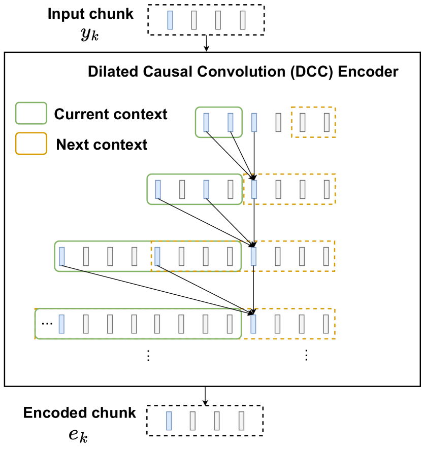
(b) DCC Encoder

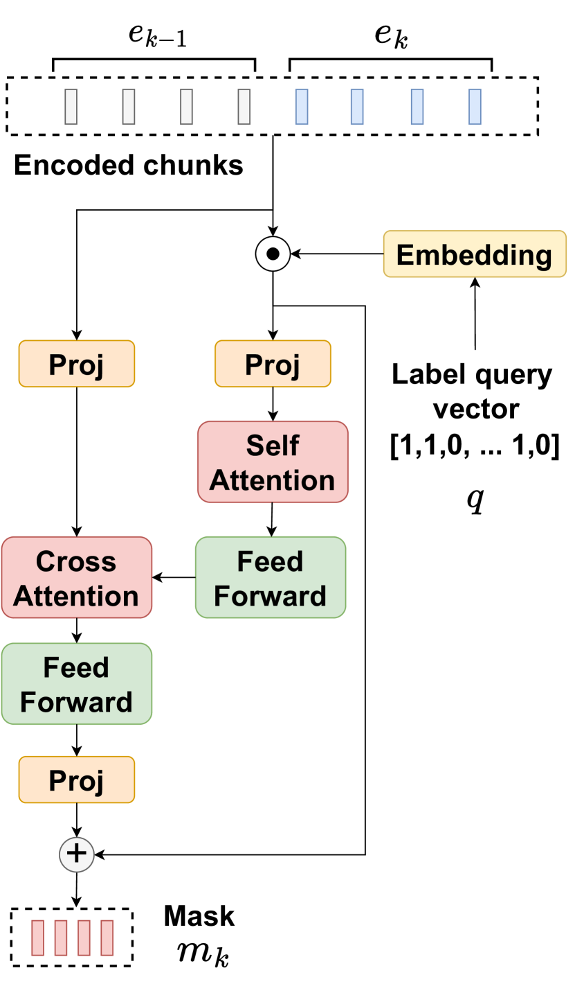
(c) Transformer Decoder

Fig. 1: Waveformer architecture. Streaming inference demonstrated using an example input mixture segment of length $4L$ samples, corresponding to a chunk length $K=4$. The query is a one-hot or a multi-hot label encoding. The Dilated Causal Convolution (DCC) encoder encodes the input chunk $y_{k}$ using the context computed from the receptive field. The transformer decoder computes the target mask by attending to current and previous encoded chunks.

2 Related work

Universal sound separation. The task here is to decompose a mixture of arbitrary sound types into their component sounds, regardless of the number of sounds in the mixture [12]. This becomes increasingly challenging as the number of possible sound types in the mixture increases. Several networks have been proposed for this task including convolutional long short-term memory networks [12], time-dilated convolution networks [12] based on Conv-TasNet [7], and transformer networks [13]. Prior work also proposed the use of embeddings learned by a sound classifier trained on a large sound ontology [14] for conditioning a separation network.

Target sound extraction. This approach can circumvent the challenge of universal sound separation struggling to deal with a mixture of a large number of sounds. The clues may be provided as an embedding of an audio clip [3, 4], an image [5, 6], natural language text [15, 16], onomatopoeic words [17], or a one-hot sound label vector [1]. The prior works [18, 19] have also evaluated the use of a sound event detector to detect the time when the target sound occurs in a mixture. Although these works are often motivated for practical usage [16, 1], none of them use streaming models. In contrast to these prior works, we design the first streaming network for target sound extraction using attention.

Speech-specific networks. Prior work has also focused on speech enhancement [20, 21, 22], speech separation [7, 23, 24, 25, 26, 27, 28] and speech selection using clues provided to the network [29, 30, 31, 32]. For speech enhancement, neural networks have been proposed [21, 33] to realize real-time operation. Recently, efficient transformer-based architectures have been proposed for speech recognition and separation tasks  [34, 11, 35]. These methods either use standard transformer blocks [10] or convolution-augmented transformer blocks [11, 35]. In contrast, we use DCC layers along with the transformer decoder. Recent work on ReSepformer [10] proposed a causal mode for their transformer method, which we use for our baseline comparisons.

3 Waveformer Architecture

We process individual audio chunks of duration $\tau$ seconds. For streaming, we need to operate at the chunk level: an output chunk can depend on the current and past chunks. Thus, streaming models have an intrinsic latency equal to the duration of a single chunk. In real-time practical systems, it is desirable that this latency is on the order of 10 ms [36]. Fig. 1 shows our proposed time-domain model architecture, which employs an encoder-decoder based mask generation network to generate an element-wise multiplicative mask in the latent space. Let $x_{k}\in R^{S}$ denote the current input audio chunk, where $S=\tau F_{s}$ is the number of audio samples included in the current chunk with a sampling rate of $F_{s}$. In the first step, a 1D-convolution layer with stride $L$ and kernel size $3L$ is applied to the input audio chunk $x_{k}$ to obtain the latent space representation, $y_{k}\in R^{E\times K}$, where $E$ is the latent space feature dimensions and $K=\frac{S}{L}$ is the feature sequence length in the latent space. Setting the kernel size to $3L$ and stride to $L$ requires an overlap of $L$ samples with the previous and the future chunk, resulting in a lookahead of $2L$ samples. In our experiments, we set $L=32$ samples at 44.1 kHz. This results in a lookahead of around $1.45$ ms, which is negligible. Given a one-hot or multi-hot query vector $q\in\{0,1\}^{N_{c}}$, where $N_{c}$ is the total number of classes, streaming target sound extraction is achieved by computing feature masks $m_{k}\in R^{E\times K}$. With the mask generation network and element-wise multiplication denoted as $\mathcal{M}$ and $\odot$, respectively, the target sound signal, $\hat{x}_{k}\in R^{S}$, is computed as:

$$y_{k}= \text{Conv1d}(x_{k}),~{}~{}~{}m_{k}=\mathcal{M}(y_{k}\ |\ y_{k-1},..,y_{2},y_{1},q)$$

$$\hat{x}_{k}= \text{ConvTranspose1d}(y_{k}\odot m_{k}).$$

3.1 Dilated causal convolution encoder

Our encoder is a stack of dilated causal convolution (DCC) layers [9], and the decoder is a transformer network [8]. The motivation for such an architecture is that the encoder computes a contextful representation of the input chunk, considering the previous chunks up to a certain receptive field, and the decoder conditions the encoder output with the query vector to estimate the target mask. While recent transformer models for speech separation [34, 10] have demonstrated performance gains over convolution-based methods [7], the latter have generally been more computationally efficient.

We attribute this efficiency gap to the difference in the way existing transformer models process the receptive field compared to convolution-based architectures. To achieve a receptive field of length $R$, given the chunk-based processing in existing transformer architectures, each chunk individually attends to all previous chunks in the receptive field resulting in $\mathcal{O}(R)$ complexity. In contrast, convolution based models [9, 7] using a stack of $M$ DCC layers with kernel size $P$ and exponentially scaling dilation factors $\{2^{0},2^{1},2^{2},...,2^{M-1}\}$ have a receptive field of $(P-1)\cdot(2^{M}-1)$. Its complexity is $\mathcal{O}(PM)$. With a small kernel size $P$, the computational complexity of the stacked DCC layers is $\mathcal{O}(P\cdot\log~{}(1+\frac{R}{P-1}))$ $\sim$ $\mathcal{O}(\log R)$ for it to have a receptive field of length $R$.

We use 10 DCC layers with a kernel size of 3 and dilation factors $\{2^{0},2^{1},2^{2},...,2^{10-1}\}$ in our encoder, resulting in a receptive field of $(3-1)\cdot(2^{10}-1)=2046$ samples in the latent space. With the initial input convolution stride $L$ set to 0.73 ms, our encoder’s receptive field is $\approx 1.5s$. Fig. 1 (b) shows an encoding of an input chunk of length 4. For chunk-based streaming inference, the encoder maintains a context buffer for each DCC layer. This context is initially computed from the $1s$ receptive field and then updated dynamically after encoding each subsequent chunk. For encoding a chunk, each DCC layer is fed with the output chunk of the previous layer, left padded with the context of length twice the layer’s dilation. After encoding a chunk, the context is updated with the rightmost elements of the padded input for it to be used in encoding the next chunk. For each input chunk $y_{k}$, the DCC encoder computes an encoded representation, $e_{k}\in R^{E\times K}$.

3.2 Query-conditioned transformer decoder

To get the mask, the encoded representation computed above must be conditioned with the query, $q$. To this end, we first compute an embedding, $l\in R^{E\times 1}$, corresponding to $q$. This is achieved by using an embedding layer comprising three 512-dimensional feed-forward sub-layers with an $N_{C}$-dimensional input and an $E$-dimensional output. Our transformer decoder conditions the encoded chunk $e_{k}$ with the query embedding $l$ and derives the mask as follows.

Fig. 1 (c) shows our decoder architecture. First, we perform multiplicative query integration [1, 3] to compute the conditioned representation: ${e_{k}}^{\prime}=e_{k}\odot l$. Since transformers are more computationally expensive with higher dimensionality, we first project the encoded representations, ${e_{k}}^{\prime}$ and $e_{k}$, to the decoder dimensions $D\leq E$ with $1\times 1$ convolution. This results in projected encoded representations, ${pe}_{k},{{pe}_{k}}^{\prime}\in R^{D\times K}$. The decoded representations are then computed by passing ${{pe}_{k},{pe}_{k}}^{\prime}$ to the transformer decoder layer’s self-attention and cross-attention blocks, respectively, to obtain target mask ${pm}_{k}\in R^{D\times K}$ in the projected decoder space. It is then projected back to the encoder dimensions with another $1\times 1$ convolution layer to obtain ${m_{k}}^{\prime}\in R^{E\times K}$. Since the bottleneck caused by the projection layers might affect the flow of gradients, as depicted in the diagram, we use a skip connection immediately after the multiplicative query integration to the output of the projection layer to compute the final mask: $m_{k}={m_{k}}^{\prime}+{e_{k}}^{\prime}$.

Within the decoder, we use the chunk-based streaming attention scheme proposed in [37]. As shown in Fig. 1(c), for decoding the current chunk, $e_{k}$, the transformer decoder only attends to the samples in the current chunk, $e_{k}$, and one previous chunk, $e_{k-1}$. This ensures that the input length to the transformer decoder is fixed at $2K$ (current chunk + one previous chunk) and prevents the inference time from growing as the input audio length increases.

Table 1: Performance on the single-target extraction task. In our model, $E$ and $D$ correspond to encoder and decoder dimensionalities, respectively. RTF is the real-time factor for a consumer CPU.

Model	Model size	RTF	SI-SNRi
Conv-TasNet	4.57M	1.34	6.14
ReSepformer	13.24M	1.60	7.26
Ours ($E=256;~{}D=128$)	1.10M	0.66	9.02
Ours ($E=256;~{}D=256$)	1.69M	0.75	9.40
Ours ($E=512;~{}D=128$)	3.29M	0.88	9.26
Ours ($E=512;~{}D=256$)	3.88M	0.94	9.43

Table 2: SI-SNRi comparison in the multi-target extraction task.

	# selected classes
Model	1	2	3	Mean
Conv-TasNet	7.20	3.63	0.19	3.67
ReSepformer	7.42	3.56	0.33	3.77
Ours ($E=256;~{}D=128$)	9.06	4.78	1.51	5.11
Ours ($E=256;~{}D=256$)	9.12	4.76	1.31	5.06
Ours ($E=512;~{}D=128$)	9.39	4.92	1.39	5.23
Ours ($E=512;~{}D=256$)	9.29	4.92	1.35	5.19

4 Experiments and results

Dataset. We use a synthetic sound mixture dataset created from the FSD Kaggle 2018 dataset [38]. FSD Kaggle 2018 is a set of sound event and class label pairs, with 41 different sound classes, which are a subset of the Audioset ontology [14]. Our synthetic dataset consists of 50k training samples, 5k validation samples, and 10k test samples. Sound mixtures are created using the Scaper toolkit [39] with FSD Kaggle 2018 and TAU Urban Acoustic Scenes 2019  [40] as foreground and background sources, respectively. Foreground sound classes are randomly sampled without replacement so that each sample has 3-5 unique classes. We construct the sound mixtures by sampling 3-5s crops from each foreground sound and then pasting them on a 6s background sound. The SNRs of the foreground sounds are randomly chosen between 15 and 25 dB, relative to the background sound. Our training and validation data are sampled from the development splits of FSD Kaggle 2018 and TAU Urban Acoustic Scenes 2019, while our test samples are from the test splits. From each mixture, up to 3 foreground sounds are randomly selected as targets. During training, the choices of the target foreground sounds in the training set are randomized. Since we mainly consider human listening applications for streaming target sound extraction, we run our experiments at a 44.1 kHz sampling rate to cover the full audible range.

(a) Input mixture

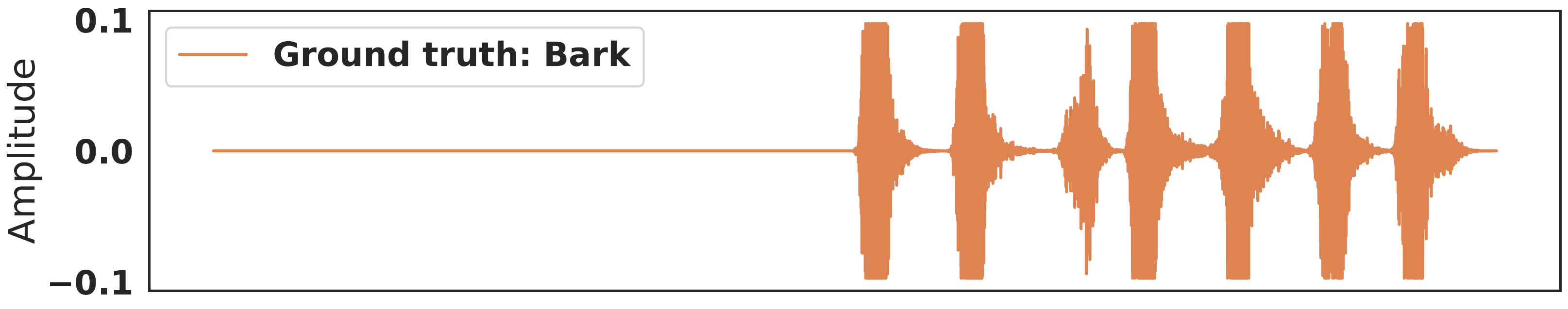
(b) Ground-truth for label ‘Bark’

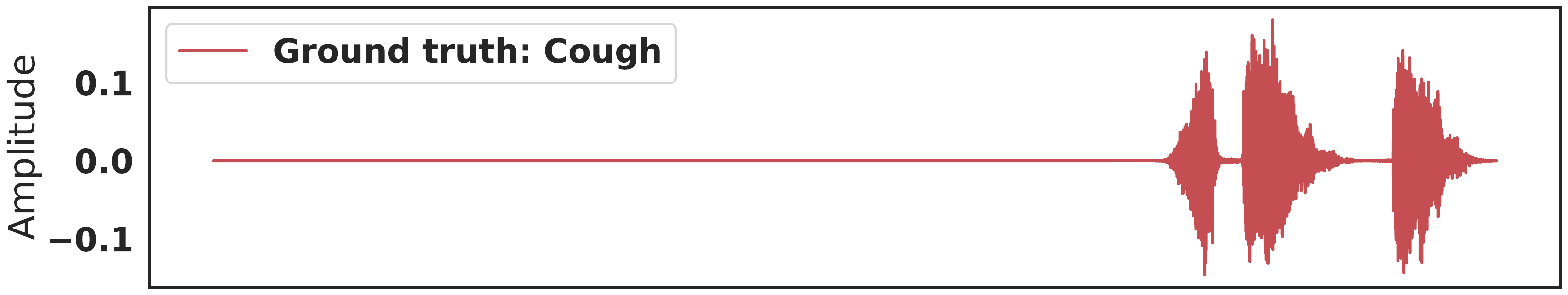
(c) Ground-truth for label ‘Cough’

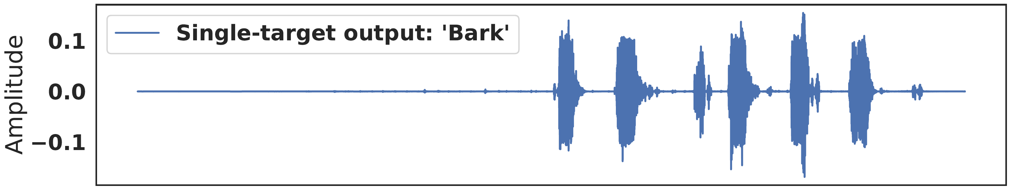
(d) Output of the single-target extraction of ‘Bark’

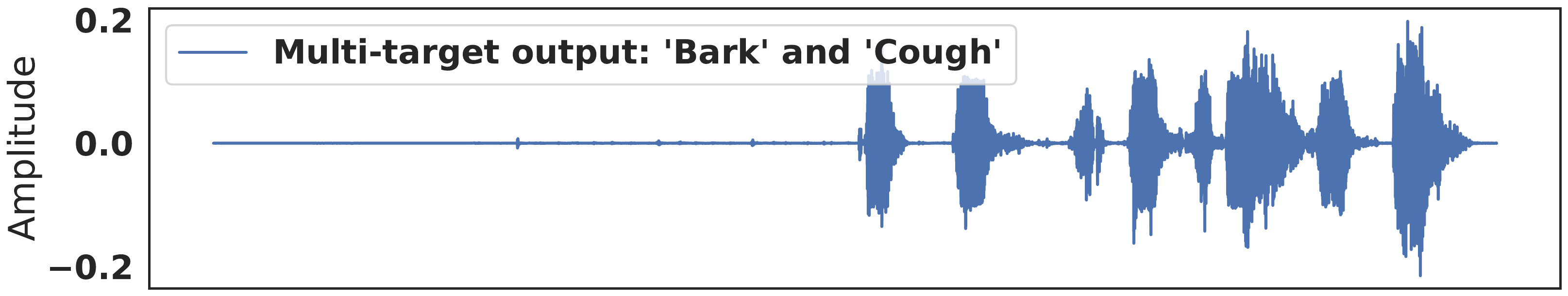
(e) Output of the multi-target extraction of ‘Bark’ and ‘Cough’

Fig. 2: Visualization of time-domain waveforms of single-target and multi-target extraction (x-axis represents time).

Evaluation setup. Prior works [1, 3] show that Conv-TasNet, originally proposed for speech separation, can also be used for target sound extraction. Further, ReSepformer proposes an efficient transformer architecture for speech separation that allows a streaming inference. Here, we compare the performance of our architecture with the causal or streaming implementations of Conv-TasNet and ReSepformer as described in the original papers [7, 10] for the target sound extraction task.

For all the models, we set the stride of the initial convolution, $L$, to 32, which is about $0.73$ ms at 44.1 kHz. We train multiple configurations of our model with different encoder and decoder dimensions. We fix the number of DCC layers to 10, the number of transformer layers to 1, and the chunk length, $K$, to 13. This chunk length corresponds to 416 samples in the time domain or a chunk duration of 9.43 ms. For Conv-TasNet, we follow the configuration used in [1] except for the number of repeats, which we set to 2. This ensures that the runtime of the Conv-TasNet baseline is not too large compared with that of our model’s largest configuration. For the ReSepformer baseline, we set the model dimensionality to 512, the number of blocks to 2, the number of transformer layers to 2, and the chunk size to 13 (9.43 ms). We perform label integration after the first transformer block, as we found it to perform better than integrating it at the beginning.

Loss function and training hyper-parameters. We use a linear combination of 90% signal-to-noise-ratio (SNR) and 10% scale-invariant-signal-to-noise-ratio (SI-SNR) [41] as the loss function for training. We set the initial learning rate to 5e-4 for our models and Conv-TasNet, and to 1.5e-4 for ReSepformer. We train the models for 100 epochs and choose the model after the epoch that resulted in the best validation SI-SNRi.

Results. We separately train the models for single-target and multi-target extraction tasks and evaluate them on our testset. For multi-target evaluation, we train our model as well as baselines to make predictions with multi-hot query vectors, as opposed to one-hot queries used in the single-target evaluation. During the multi-target training, 1-3 foreground sounds are randomly selected as target sounds. This training method using an arbitrary number of target sources helps the model learn multi-target embeddings. The same model configurations are used for both the single-target and multi-target experiments. The Conv-TasNet and ReSepfromer baselines are also trained in the same way for the multi-target extraction task.

We also evaluate the real-time factors (RTFs) of the models on an Intel Core i5 CPU using a single thread. RTF is computed by measuring the runtime consumed by the models to process a 416 sample audio chunk (9.43 ms at 44.1 kHz), and dividing that by the chunk duration, 9.43 ms. For the RTF measurement, we include the padding for dilated convolution layers in our model’s DCC encoder and Conv-TasNet’s Temporal Convolution Network (TCN) blocks, accounting for the entire receptive field. In the case of the ReSepformer, using a single chunk for RTF measurement excludes the overhead caused by causal attention masking in its inter-attention blocks. Consequently, the RTF value reported for ReSepformer is a lower bound of what is practically achievable.

Table 1 compares our models with different configurations with the baselines in terms of both efficiency and performance. We show that our approach results in 2.2-3.3 dB SI-SNRi improvement compared with the baselines while being 1.5-2x more computationally efficient with 1.2-4x fewer parameters. Table 2 compares the performance of our models with the baselines for the multiple target extraction task. It shows that our method outperforms the baselines by 1.2-1.4 dB for the 2-target case and 1-1.2 dB for the 3-target case. As with prior work [1], the SI-SNR improvements are lower in the 3-target selection task since there is greater similarity between the input mixture and the target signal, compared to the single-target case, resulting in a larger input SI-SNR. We obtained $p$-values $<0.05$ for all comparisons except for the comparison between $(E=512;D=256)$ and $(E=256;D=256)$, for which the $p$-value was $0.57$.

In Fig. 2, we qualitatively show an example of single-target extraction and multi-target extraction from a 4-class input mixture, using our multi-target extraction model. Fig. 2(a) shows the input mixture waveform, and Figs. 2(b) and 2(c) show the isolated ground-truth sounds. We provide the input mixture to our multi-target model, with a single-target query followed by a two-target query. Figs. 2(d) and 2(e) are the output waveforms obtained when the single target and the two targets are queried, respectively. The waveforms show that the model successfully recognizes the queried events and extracts the relevant sounds. It can also be observed that our model preserves the original amplitudes of the sounds in the input mixture well.

We also implemented a non-causal version of the proposed Waveformer. The dilated causal convolution (DCC) block was made non-causal by padding on both sides of each DCC layer’s input sequence, while the causal version only padded to the left. The non-causal transformer decoder attends to the previous and next chunks, in addition to the current chunk. Following [1], we trained our non-causal model with both one-hot/multi-hot based extraction and Permutation Invariant Training + Oracle Selection (PIT + OS) objectives. Table 3 compares the performance of the non-causal version of our model with non-causal baselines. The performance of our causal model is only 1.1 dB less than the non-causal version, in contrast, to the 3–5 dB observed in prior source separation works [7, 10]. We achieve this resilience by using layer normalization throughout our architecture (avoiding the gLN to cLN switch in [7, 10]) and a small context length for the transformer decoder.

Table 3: Performance comparison with non-causal baselines.

Model	SI-SNRi
Listen to What You Want [1]	9.91
Ours ($E=512;~{}D=256$; Non-causal)	10.50
Ours ($E=512;~{}D=256$; Non-causal; PIT+OS)	11.31

5 Conclusions

We demonstrate the first deep learning method for real-time and streaming target sound extraction. Future work includes the use of more constrained computing platforms, larger datasets with more classes, and multiple microphones. Our Waveformer architecture may be applicable to other acoustic applications like source separation and directional hearing, which deserves further exploration.

Acknowledgements. The UW researchers are funded by the Moore Inventor Fellow award #10617 and the National Science Foundation.

References

- [1] T. Ochiai, M. Delcroix, Y. Koizumi, H. Ito, K. Kinoshita, and S. Araki, “Listen to What You Want: Neural Network-based Universal Sound Selector,” arXiv e-prints, p. arXiv:2006.05712, 2020.
- [2] M. Delcroix, J. B. Vázquez, T. Ochiai, K. Kinoshita, and S. Araki, “Few-shot learning of new sound classes for target sound extraction,” arXiv preprint arXiv:2106.07144, 2021.
- [3] M. Delcroix, J. B. Vázquez, T. Ochiai, K. Kinoshita, Y. Ohishi, and S. Araki, “Soundbeam: Target sound extraction conditioned on sound-class labels and enrollment clues for increased performance and continuous learning,” arXiv preprint arXiv:2204.03895, 2022.
- [4] B. Gfeller, D. Roblek, and M. Tagliasacchi, “One-shot conditional audio filtering of arbitrary sounds,” in ICASSP. IEEE, 2021.
- [5] R. Gao and K. Grauman, “Co-separating sounds of visual objects,” in Proceedings of the IEEE/CVF International Conference on Computer Vision, 2019.
- [6] X. Xu, B. Dai, and D. Lin, “Recursive visual sound separation using minus-plus net,” in IEEE/CVF ICCV, 2019.
- [7] Y. Luo and N. Mesgarani, “Conv-tasnet: Surpassing ideal time–frequency magnitude masking for speech separation,” IEEE/ACM transactions on audio, speech, and language processing, vol. 27, no. 8, 2019.
- [8] A. Vaswani, N. Shazeer, N. Parmar, J. Uszkoreit, L. Jones, A. N. Gomez, L. Kaiser, and I. Polosukhin, “Attention is all you need,” 2017.
- [9] A. v. d. Oord, S. Dieleman, H. Zen, K. Simonyan, O. Vinyals, A. Graves, N. Kalchbrenner, A. Senior, and K. Kavukcuoglu, “Wavenet: A generative model for raw audio,” 2016.
- [10] C. Subakan, M. Ravanelli, S. Cornell, F. Lepoutre, and F. Grondin, “Resource-efficient separation transformer,” arXiv preprint arXiv:2206.09507, 2022.
- [11] J. Luo, J. Wang, N. Cheng, E. Xiao, X. Zhang, and J. Xiao, “Tiny-sepformer: A tiny time-domain transformer network for speech separation,” arXiv preprint arXiv:2206.13689, 2022.
- [12] I. Kavalerov, S. Wisdom, H. Erdogan, B. Patton, K. Wilson, J. Le Roux, and J. R. Hershey, “Universal sound separation,” in 2019 WASPAA. IEEE, 2019.
- [13] A. Zadeh, T. Ma, S. Poria, and L.-P. Morency, “Wildmix dataset and spectro-temporal transformer model for monoaural audio source separation,” arXiv preprint arXiv:1911.09783, 2019.
- [14] J. F. Gemmeke, D. P. Ellis, D. Freedman, A. Jansen, W. Lawrence, R. C. Moore, M. Plakal, and M. Ritter, “Audio set: An ontology and human-labeled dataset for audio events,” in ICASSP. IEEE, 2017.
- [15] K. Kilgour, B. Gfeller, Q. Huang, A. Jansen, S. Wisdom, and M. Tagliasacchi, “Text-driven separation of arbitrary sounds,” arXiv preprint arXiv:2204.05738, 2022.
- [16] X. Liu, H. Liu, Q. Kong, X. Mei, J. Zhao, Q. Huang, M. D. Plumbley, and W. Wang, “Separate what you describe: Language-queried audio source separation,” arXiv preprint arXiv:2203.15147, 2022.
- [17] Y. Okamoto, S. Horiguchi, M. Yamamoto, K. Imoto, and Y. Kawaguchi, “Environmental sound extraction using onomatopoeic words,” in ICASSP. IEEE, 2022.
- [18] Q. Kong, Y. Wang, X. Song, Y. Cao, W. Wang, and M. D. Plumbley, “Source separation with weakly labelled data: An approach to computational auditory scene analysis,” in ICASSP. IEEE, 2020.
- [19] K. Chen, X. Du, B. Zhu, Z. Ma, T. Berg-Kirkpatrick, and S. Dubnov, “Zero-shot audio source separation through query-based learning from weakly-labeled data,” in AAAI, 2022, vol. 36.
- [20] S. Wisdom, J. R. Hershey, K. Wilson, J. Thorpe, M. Chinen, B. Patton, and R. A. Saurous, “Differentiable consistency constraints for improved deep speech enhancement,” in ICASSP. IEEE, 2019.
- [21] S. E. Eskimez, T. Yoshioka, H. Wang, X. Wang, Z. Chen, and X. Huang, “Personalized speech enhancement: New models and comprehensive evaluation,” in ICASSP. IEEE, 2022.
- [22] I. Chatterjee, M. Kim, V. Jayaram, S. Gollakota, I. Kemelmacher, S. Patel, and S. M. Seitz, “Clearbuds: wireless binaural earbuds for learning-based speech enhancement,” in MobiSys, 2022.
- [23] Y. Luo, Z. Chen, and T. Yoshioka, “Dual-path RNN: efficient long sequence modeling for time-domain single-channel speech separation,” in ICASSP. IEEE, 2020.
- [24] P.-S. Huang, M. Kim, M. Hasegawa-Johnson, and P. Smaragdis, “Deep learning for monaural speech separation,” in ICASSP. IEEE, 2014.
- [25] J. R. Hershey, Z. Chen, J. Le Roux, and S. Watanabe, “Deep clustering: Discriminative embeddings for segmentation and separation,” in ICASSP. IEEE, 2016.
- [26] Y. Isik, J. L. Roux, Z. Chen, S. Watanabe, and J. R. Hershey, “Single-channel multi-speaker separation using deep clustering,” arXiv preprint arXiv:1607.02173, 2016.
- [27] D. Yu, M. Kolbæk, Z.-H. Tan, and J. Jensen, “Permutation invariant training of deep models for speaker-independent multi-talker speech separation,” in ICASSP. IEEE, 2017.
- [28] Q. Wang, H. Muckenhirn, K. Wilson, P. Sridhar, Z. Wu, J. Hershey, R. A. Saurous, R. J. Weiss, Y. Jia, and I. L. Moreno, “Voicefilter: Targeted voice separation by speaker-conditioned spectrogram masking,” arXiv preprint arXiv:1810.04826, 2018.
- [29] E. Tzinis, G. Wichern, A. Subramanian, P. Smaragdis, and J. L. Roux, “Heterogeneous target speech separation,” arXiv preprint arXiv:2204.03594, 2022.
- [30] A. Ephrat, I. Mosseri, O. Lang, T. Dekel, K. Wilson, A. Hassidim, W. T. Freeman, and M. Rubinstein, “Looking to listen at the cocktail party: A speaker-independent audio-visual model for speech separation,” arXiv preprint arXiv:1804.03619, 2018.
- [31] A. Wang, M. Kim, H. Zhang, and S. Gollakota, “Hybrid neural networks for on-device directional hearing,” AAAI, vol. 36, no. 10, 2022.
- [32] Z. Wang, R. Giri, S. Venkataramani, U. Isik, J.-M. Valin, P. Smaragdis, M. Goodwin, and A. Krishnaswamy, “Semi-supervised time domain target speaker extraction with attention,” arXiv preprint arXiv:2206.09072, 2022.
- [33] R. Giri, S. Venkataramani, J.-M. Valin, U. Isik, and A. Krishnaswamy, “Personalized percepnet: Real-time, low-complexity target voice separation and enhancement,” arXiv preprint arXiv:2106.04129, 2021.
- [34] C. Subakan, M. Ravanelli, S. Cornell, M. Bronzi, and J. Zhong, “Attention is all you need in speech separation,” in ICASSP. IEEE, 2021.
- [35] A. Gulati, J. Qin, C.-C. Chiu, N. Parmar, Y. Zhang, J. Yu, W. Han, S. Wang, Z. Zhang, Y. Wu, and R. Pang, “Conformer: Convolution-augmented transformer for speech recognition,” 2020.
- [36] M. Sunohara, C. Haruta, and N. Ono, “Low-latency real-time blind source separation for hearing aids based on time-domain implementation of online independent vector analysis with truncation of non-causal components,” in ICASSP, 2017.
- [37] X. Chen, Y. Wu, Z. Wang, S. Liu, and J. Li, “Developing real-time streaming transformer transducer for speech recognition on large-scale dataset,” in ICASSP 2021 - 2021 IEEE International Conference on Acoustics, Speech and Signal Processing (ICASSP), 2021, pp. 5904–5908.
- [38] E. Fonseca, M. Plakal, F. Font, D. P. W. Ellis, X. Favory, J. Pons, and X. Serra, “General-purpose tagging of freesound audio with audioset labels: Task description, dataset, and baseline,” in DCASE2018, November 2018.
- [39] J. Salamon, D. MacConnell, M. Cartwright, P. Li, and J. P. Bello, “Scaper: A library for soundscape synthesis and augmentation,” in WASPAA, 2017.
- [40] A. Mesaros, T. Heittola, and T. Virtanen, “A multi-device dataset for urban acoustic scene classification,” in DCASE2018, November 2018.
- [41] J. L. Roux, S. Wisdom, H. Erdogan, and J. R. Hershey, “SDR - half-baked or well done?,” 2018.