Divergent stiffness of one-dimensional growing interfaces

Abstract

When a spatially localized stress is applied to a growing one-dimensional interface, the interface deforms. This deformation is described by the effective surface tension representing the stiffness of the interface. We present that the stiffness exhibits divergent behavior in the large system size limit for a growing interface with thermal noise, which has never been observed for equilibrium interfaces. Furthermore, by connecting the effective surface tension with a space-time correlation function, we elucidate the mechanism that anomalous dynamical fluctuations lead to divergent stiffness.

Introduction.— The statistical behavior of many-interacting elements out of equilibrium has attracted attention for a wide range of systems [3, 1, 2]. A remarkable feature of such systems is that the standard relations in equilibrium systems no longer hold. For example, phase order in two dimensions is not observed for equilibrium systems at finite temperatures [5, 4], while it emerges for active matters [6] or sheared systems [7]. The particular nature of out-of-equilibrium systems is not limited to phase transition problems. The phenomenon we study in this Letter is the singular response against a perturbation.

In studying response properties of equilibrium systems, the fluctuation response relation is useful. That is, the static response against a perturbation is connected to static fluctuation properties in the system without perturbation. As a result of this relation, the response is found to be finite except for phase transition points because static fluctuations are normal in general. In contrast, the static response against a perturbation imposed to a non-equilibrium steady state is not determined by static fluctuation properties. Although several expressions of the static response for out-of-equilibrium systems have been proposed [8, 9, 10, 11, 12, 13] and experimentally studied [14, 15, 16] for the last two decades, the most primitive method is to consider the time evolution of the perturbation [17, 18, 19]. This means that the dynamic properties of fluctuations influence the static response if there is no special property such as a detailed balance condition. Therefore, a singular response behavior can be observed without tuning system conditions.

To demonstrate the singular response of many interacting elements out of equilibrium, we specifically study a one-dimensional interface, whose height is defined in $0\leq x\leq L$. The interface deforms when a localized stress is applied. For equilibrium interfaces [20], which do not grow but fluctuate in an equilibrium environment, their mean profile in the linear response regime is expressed by a quadratic function of $x$, where its curvature is determined by the surface tension $\kappa$. Now, let us consider growing interfaces [21]. We can numerically confirm that the deformation against the weak localized stress is still described by a quadratic function of $x$. In this case, the curvature of the interface is characterized by the effective surface tension $\kappa_{\rm eff}$. We then find that $\kappa_{\rm eff}$ diverges as $L\to\infty$. In other words, growing interfaces exhibit divergent stiffness.

We attempt to explore the mechanism of the divergent stiffness by formulating a fluctuation-response relation. This problem is reminiscent of the standard linear response theory around an equilibrium state. For example, when considering heat conduction for a Hamiltonian system in contact with two heat baths with temperatures $T_{1}$ and $T_{2}$, $T_{2}-T_{1}$ is treated as a perturbation [22]. In this case, the linear response formula is the Green-Kubo formula, which expresses the conductivity in terms of the time integration of the current correlation function at equilibrium [19]. Similarly to heat conduction, we expect that the effective surface tension $\kappa_{\rm eff}$ can be expressed as the time integration of a certain time correlation function. In this Letter, we derive such a formula using a generalized fluctuation theorem associated with the excess entropy production.

Based on the response formula, we study the divergent stiffness. As is known, some low-dimensional systems exhibit an anomaly in the large-distance and long-time properties of the time correlation function [22]. In such systems, the decay rate of a time correlation function is so small that its time integration is not bounded in the large system size limit [23, 22, 24]. By combining this property with the response formula, the mechanism of the divergent stiffness is understood. We emphasize that the method we propose in this Letter can be applied to other spatially extended systems out-of-equilibrium.

Setup.— The one-dimensional interface defined in $0\leq x\leq L$ is investigated. The height of the interface at time $t$ is expressed by $h(x,t)$, which is collectively denoted by $\hat{h}=(h(x))_{x=0}^{L}$. For simplicity, the periodic boundary condition $h(0,t)=h(L,t)$ is assumed. An external stress $\epsilon p_{{\rm ex}}(x)$ is imposed on the interface, where the total force $\epsilon\int p_{{\rm ex}}(x)dx$ is set to zero to avoid the additional drift of the interface. We first study an equilibrium interface. The free energy of the interface is assumed to be

$$F^{\epsilon}(\hat{h})\equiv\int_{0}^{L}dx\left[\frac{\kappa}{2}(\partial_{x}h)^{2}-\epsilon p_{{\rm ex}}(x)h(x)\right],$$ (1)

where $\kappa$ represents the surface tension. The fluctuation properties are described by the following stochastic model [20]:

$$\partial_{t}h=-\frac{1}{\gamma}\frac{\delta F^{\epsilon}(\hat{h})}{\delta h}+\sqrt{\frac{2T}{\gamma}}\xi,$$ (2)

where $\gamma$ is the dissipation constant; $T$ is the temperature of the bath with the Boltzmann constant set to unity; $\xi$ is the Gaussian white noise satisfying

$$\left\langle\xi(x,t)\xi(x^{\prime},t^{\prime})\right\rangle=\delta(x-x^{\prime})\delta(t-t^{\prime}).$$ (3)

Thus, it is immediately confirmed that the expectation of the interface shape under the external stress is given by

$$\kappa\partial_{x}^{2}\left\langle h(x)\right\rangle_{{\rm eq}}^{\epsilon}+\epsilon p_{{\rm ex}}(x)=0,$$ (4)

where $\left\langle\cdot\right\rangle_{{\rm eq}}^{\epsilon}$ denotes the expectation in the equilibrium state of the system with the external stress $\epsilon p_{\rm ex}(x)$. For simplicity, focus is placed on the case where $p_{\rm ex}(x)=\delta(x)-1/L$. By solving (4) [25], we obtain

$$\left\langle h(x)-h(0)\right\rangle_{{\rm eq}}^{\epsilon}=\frac{\epsilon}{2L\kappa}\left[\left(x-\frac{L}{2}\right)^{2}-\frac{L^{2}}{4}\right].$$ (5)

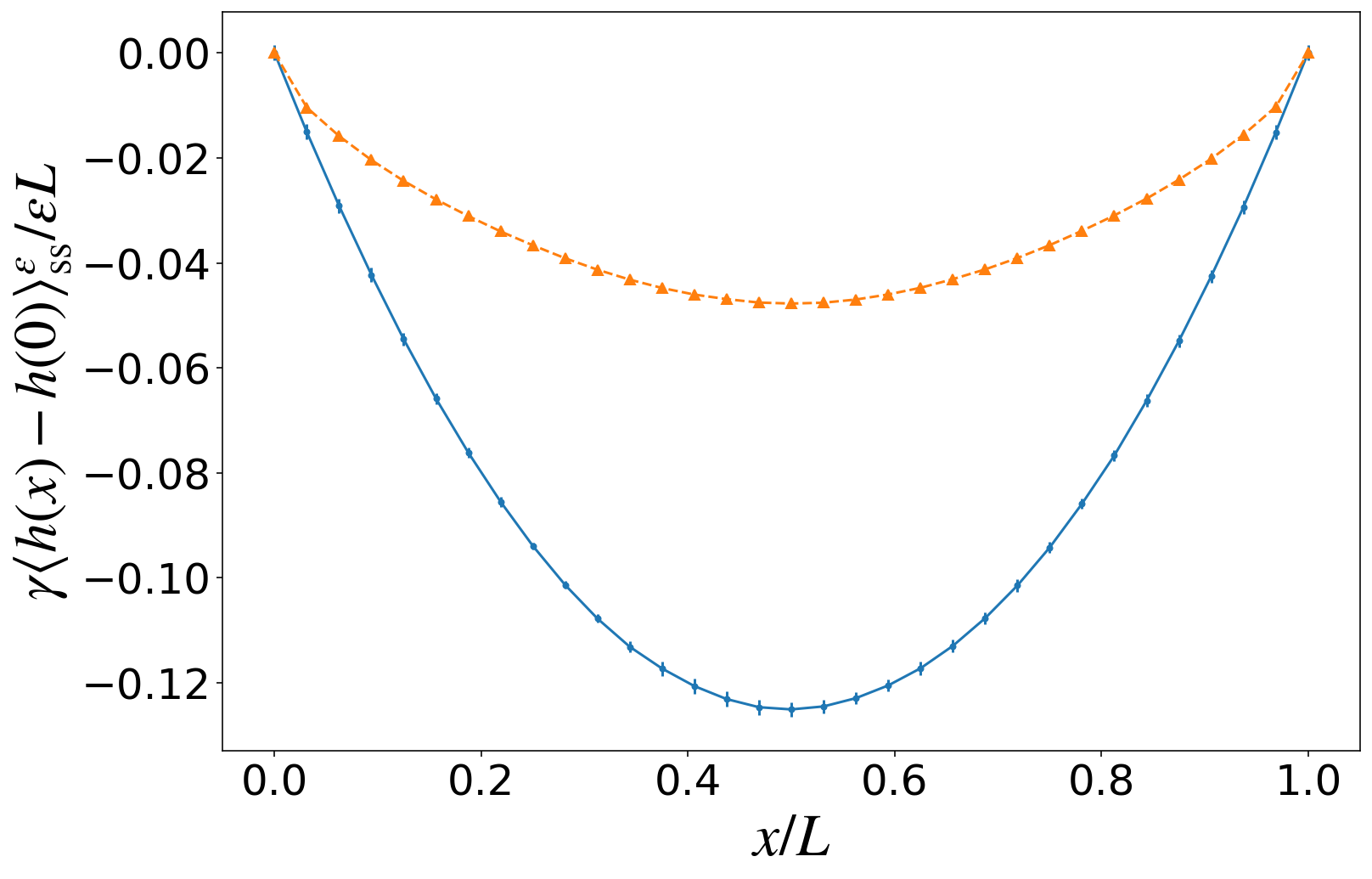
Figure 1: Time-averaged patterns in steady state under the external stress with $\epsilon/\gamma=0.01$. The system size is $L=16$. The curvature of the growing interface ($v_{0}=5$, triangular-orange symbol) is smaller than that of the equilibrium interface ($v_{0}=0$, round-blue symbol). The symbols are joined by lines for visual aid.

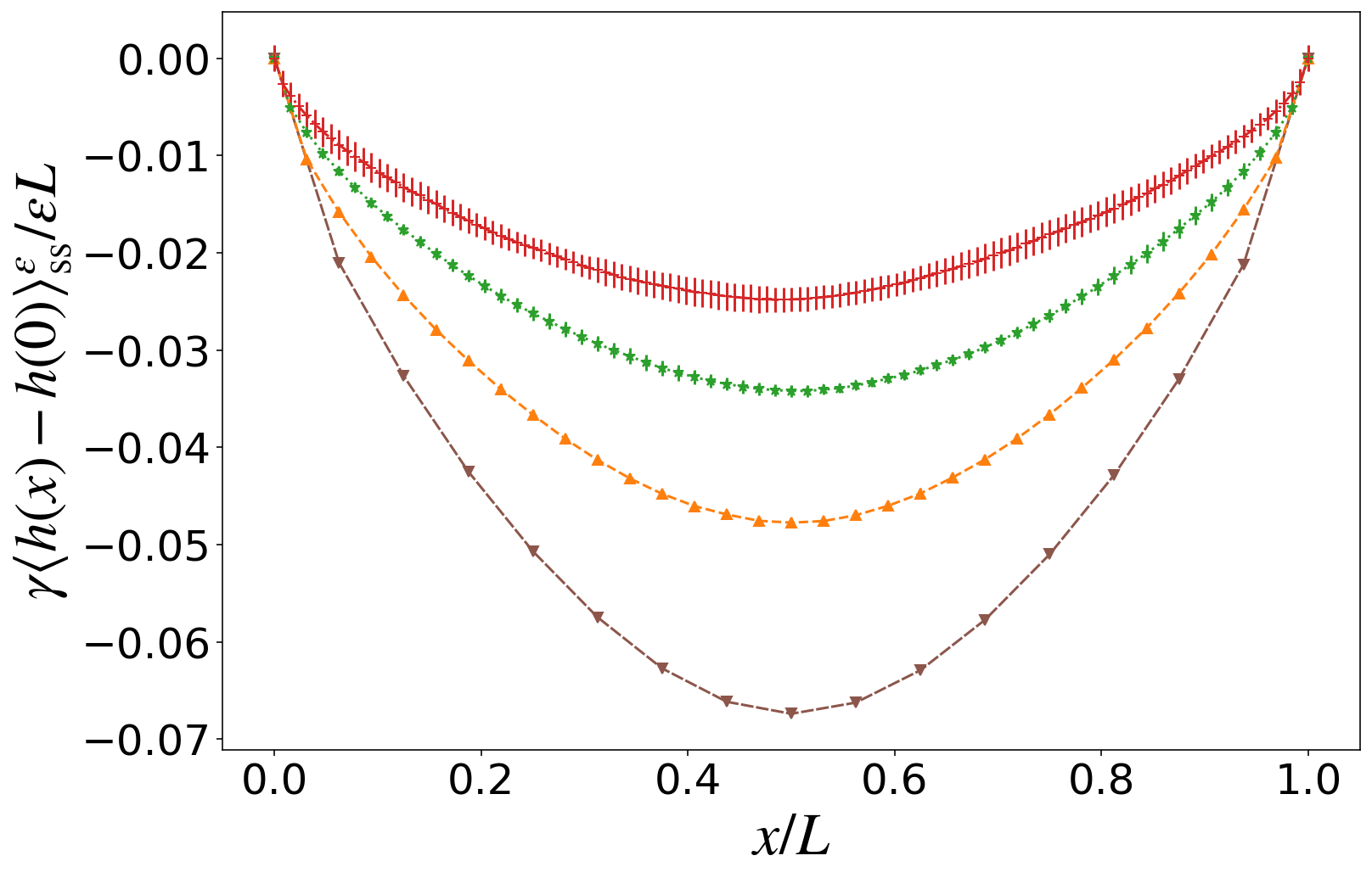
Figure 2: System size dependence of the curve for $v_{0}=5$ in Fig.1. The patterns of $L=8,16,32$, and $64$ are shown from bottom to top. The symbols are joined by lines for visual aid. Although the equilibrium ($v_{0}=0$) interface does not depend on $L$, the growing interface becomes stiffer for larger $L$.

Now, let us consider a growing interface described by

$$\partial_{t}h=v_{0}+\frac{v_{0}}{2}(\partial_{x}h)^{2}-\frac{1}{\gamma}\frac{\delta F^{\epsilon}(\hat{h})}{\delta h}+\sqrt{\frac{2T}{\gamma}}\xi,$$ (6)

as a generalization of (2), where $v_{0}\geq 0$ is the propagation velocity of the flat interface. When $\epsilon=0$, (6) is equivalent to the Kardar-Parisi-Zhang (KPZ) equation [21], which qualitatively reproduces the dynamics of growing interfaces, such as interfaces in liquid-crystal turbulence [26], slow-combustion fronts in paper [27], and fronts of growing bacterial colony [28]. Because interfaces appear at almost all scales of interest in science [2, 29], the KPZ equation has been extensively investigated through numerical [30, 31, 1, 33, 34, 35, 36], theoretical [37, 38, 39, 40, 2, 42, 43], and even mathematical [44, 45, 46, 47, 48, 49, 50, 51] approaches. The system given by (6) is interpreted as a perturbed KPZ equation.

Numerical observation.— Let $\left\langle h(x)-h(0)\right\rangle_{{\rm ss}}^{\epsilon}$ be the expectation of $h(x)-h(0)$ with respect to the steady state of (6). As an illustration, first, we numerically investigate $\left\langle h(x)-h(0)\right\rangle_{{\rm ss}}^{\epsilon}$ for the specific parameter values $\kappa=T=\gamma=1$ and $v_{0}=5$. Throughout this study, the numerical simulations were conducted using a spatially discretized model with a space interval $\Delta x=0.5$ [25, 1]. More precisely, we define a discrete model and check system size dependence to judge whether it gives a systematic approximation of the KPZ equation. The shapes of the growing interfaces shown in Fig. 2 are fitted to the following form:

$$\left\langle h(x)-h(0)\right\rangle_{{\rm ss}}^{\epsilon}=\frac{\epsilon}{2L\kappa_{{\rm eff}}}\left[\left(x-\frac{L}{2}\right)^{2}-\frac{L^{2}}{4}\right],$$ (7)

which is the generalization of (5) with the replacement of $\kappa$ by $\kappa_{{\rm eff}}$, where $\epsilon$ is assumed to be sufficiently small. The fitting parameter $\kappa_{{\rm eff}}$ is interpreted as the effective surface tension characterizing the stiffness of the growing interface. We conjecture that (7) is valid in the limit $\epsilon\to 0$ because the linear response for the noiseless case is expressed as a quadratic function [25]. Fig. 1 shows that $\kappa_{\rm eff}$ is greater than $\kappa$. Furthermore, as shown in Fig. 2, $\kappa_{\rm eff}$ increases for a larger system size $L$.

Now, two issues naturally arise. The first issue is quantifying the $L$ dependence of $\kappa_{\rm eff}$. From the viewpoint of numerical calculation, however, it becomes harder to accurately observe a slight shift of $\left<h(x)-h(0)\right>_{\rm ss}^{\epsilon}$ caused by the external stress for larger systems. The second issue is to investigate the mechanism of the $L$ dependence. Both issues can be resolved by formulating a fluctuation-response relation for the system under investigation, where $\kappa_{\rm eff}$ is expressed by dynamical properties of fluctuations in a system without the external stress.

Response formula.— Let $[\hat{h}]$ be a trajectory $(\hat{h}(t))_{t=0}^{\tau}$. We consider any quantity $A([\hat{h}])$ satisfying $A([\hat{h}+\hat{c}])=A([\hat{h}])$, where $\hat{c}$ is a constant function in $x$. For such $A([\hat{h}])$, we define $A^{*}$ as $A^{*}([\hat{h}])\equiv A([\hat{h}]^{*})$ with $[\hat{h}]^{*}\equiv(\hat{h}(\tau-t))_{t=0}^{\tau}$, which represents the time-reversal of $[\hat{h}]$. For equilibrium cases $v_{0}=0$, the detailed balance condition $\left\langle A\right\rangle_{\rm eq}^{\epsilon}=\left\langle A^{*}\right\rangle_{\rm eq}^{\epsilon}$ holds for any $\epsilon$, and the stationary distribution is given by

$$P^{\epsilon}_{\rm eq}(h)=\frac{1}{Z}\exp(-\beta F^{\epsilon}(h))$$ (8)

with $\beta=T^{-1}$. This also leads to (4).

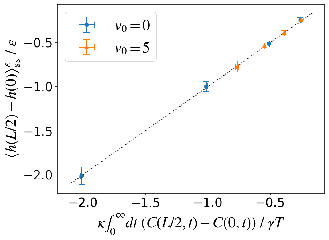
Figure 3: Comparison of the left-hand side and the right-hand side of (13). The former is estimated by the direct calculation of the response for $\epsilon>0$, while the latter is calculated in the system with $\epsilon=0$. The round-blue and triangular-orange symbols represent the data for $v_{0}=0$ ($L=2,4,8,16$) and $v_{0}=5$ ($L=2,4,8,16$), respectively. These symbols should be on the dotted line if the left and right-hand sides of (13) are equal.

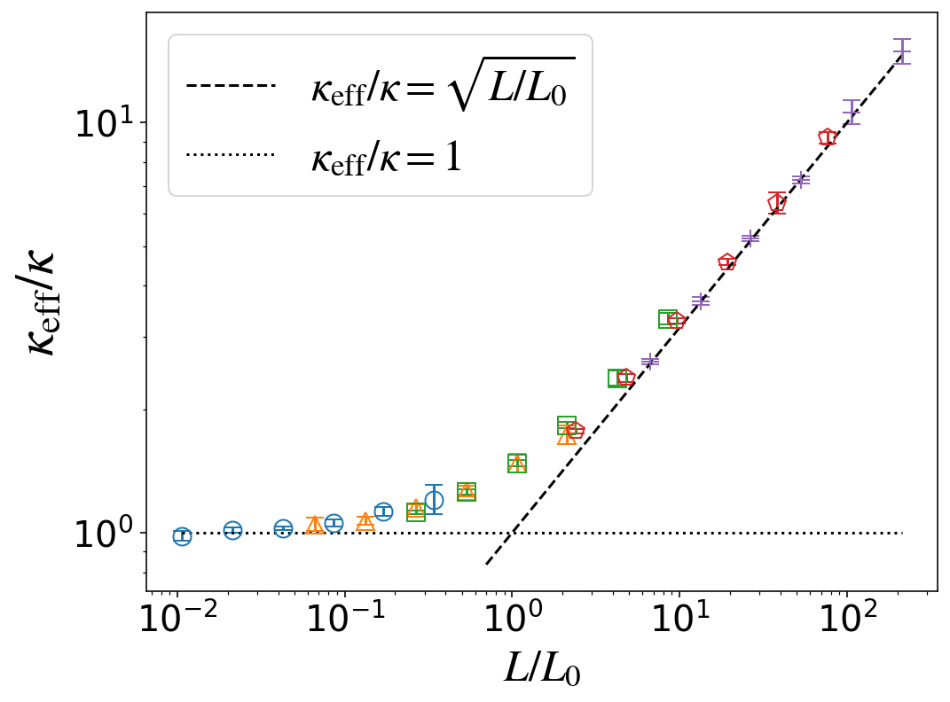
Figure 4: System size dependence of $\kappa_{\rm eff}$. The symbols are the numerical results for $L=16,32,64,128,256$, and $512$ for $v_{0}=0.2,0.5,1,3$, and $5$ from left to right (difference in symbols represents the difference in $v_{0}$). $\kappa_{\rm eff}$ maintains the same value as $\kappa$ for $L\ll L_{0}$ and diverges as $(L/L_{0})^{1/2}$ for $L\gg L_{0}$.

For growing interfaces with $v_{0}>0$, the detailed balance condition does not hold. The extent of the violation is expressed by the entropy production

$$\sigma=\frac{\gamma}{T}\int_{0}^{\tau}dt\int_{0}^{L}dx\ (\partial_{t}h)\left(v_{0}+\frac{v_{0}}{2}(\partial_{x}h)^{2}\right),$$ (9)

which is the work done by the non-conservative force divided by the temperature. Using this thermodynamic entropy production, we arrive at the standard fluctuation theorem [25]

$$\left\langle A\right\rangle_{\rm tr}^{I}=\left\langle A^{*}e^{-\sigma}\right\rangle_{\rm tr}^{I},$$ (10)

where $\left\langle\cdot\right\rangle_{\rm tr}^{I}$ denotes the ensemble average over noise realizations and the initial conditions sampled from the stationary distribution with $v_{0}=0$. This relation holds for a wide range of driven systems in contact with a heat bath [52, 53, 54, 55]. However, (S.46) is not useful to obtain the linear response property around the state with $v_{0}\not=0$ and $\epsilon=0$.

Here, we notice another time-reversal transformation $[\hat{h}]\to\$$[\hat{h}]^{\dagger}\equiv(-\hat{h}(\tau-t))_{t=0}^{\tau}$ such that $\left\langle A\right\rangle_{\rm ss}^{0}=\left\langle A^{\dagger}\right\rangle_{\rm ss}^{0}$ holds for $A^{\dagger}([\hat{h}])\equiv A([\hat{h}]^{\dagger})$ [23, 25]. However, this time-reversal symmetry is violated for interfaces under the external stress $\epsilon>0$. Then, following the standard procedure for the fluctuation theorem [55], we calculate the ratio of path probabilities of $[\hat{h}]$ and $[\hat{h}]^{\dagger}$ and take the logarithm of the result to obtain

$$\tilde{\sigma}\equiv-\frac{\epsilon\kappa}{\gamma T}\int_{0}^{\tau}dt\int_{0}^{L}dx\ p_{\rm ex}(x)\frac{\partial^{2}h(x,t)}{\partial^{2}x},$$ (11)

which characterizes the violation of the symmetry associated with the time-reversal transformation $[\hat{h}]\to[\hat{h}]^{\dagger}$. Indeed, we can show a generalized fluctuation theorem

$$\left\langle A\right\rangle_{\rm tr}^{II}=\left\langle A^{\dagger}e^{-\tilde{\sigma}}\right\rangle_{\rm tr}^{II},$$ (12)

where $\left\langle\cdot\right\rangle_{\rm tr}^{II}$ denotes the ensemble average over the noise realizations and initial conditions sampled from the stationary distribution without the external stress. Note that $\tilde{\sigma}$ is not the thermodynamic entropy production, but interpreted as an excess entropy production that appears only when the external stress is imposed [56].

Here, we set $A=h(x,\tau)-h(0,\tau)$, substitute it into (S.50), take the limit $\tau\to\infty$, and expand the right-hand side of (S.50) in $\epsilon$. Noting that $\left<A\right>^{II}_{\rm tr}$ goes to $\left<h(x)-h(0)\right>_{\rm ss}^{\epsilon}$, we obtain [25]

$$\lim_{\epsilon\to 0}\frac{\left<h(x)-h(0)\right>_{\rm ss}^{\epsilon}}{\epsilon}=\frac{\kappa}{\gamma T}\int_{0}^{\infty}dt\ \left(C(x,t)-C(0,t)\right)$$ (13)

with

$$C(x,t)\equiv\left\langle\partial_{x}h(x,0)\partial_{x}h(0,t)\right\rangle_{\rm ss}^{0}.$$ (14)

This relation is interpreted as the fluctuation-response relation of the system under investigation. (13) is understood from the fluctuation-dissipation theorem for classical stochastic processes [57, 58, 59]. However, to our best knowledge, an explicit formula connecting the response to an external perturbation has never been proposed to date. We numerically check the validity of (13) for small systems with $L=2,4,8$, and $16$. In Fig. 3, the left-hand side of (13) is plotted against the right-hand side of (13) at $x=L/2$ for both cases of $v_{0}=0$ and $v_{0}=5$. The result confirms that (13) holds.

Divergent stiffness.— As explained above, the numerical calculation of $\kappa_{{\rm eff}}$ defined by (7) is not easy to carry out for large systems. Thus, using the response formula (13), we study the stiffness of the growing interface. Specifically, from (7) and (13), we obtain

$$\kappa_{\rm eff}=-\frac{\gamma TL}{8\kappa}\left\{\int_{0}^{\infty}dt\ \left[C\left(\frac{L}{2},t\right)-C(0,t)\right]\right\}^{-1}.$$ (15)

By dimensional analysis, we find that $\kappa_{{\rm eff}}/\kappa$ is expressed as a function of $L/L_{0}$ with

$$L_{0}=\frac{\ell\kappa^{3}}{T\gamma^{2}v_{0}^{2}},$$ (16)

where $\ell$ is a numerical constant corresponding to the dimensionless length characterizing the cross-over [25]. In other words, the following equation is obtained using a scaling function $f$ whose form has not been determined yet:

$$\kappa_{\rm eff}=\kappa f\left(\frac{L}{L_{0}}\right).$$ (17)

First, we notice that $\kappa_{\rm eff}\to\kappa$ as $L_{0}\to\infty$, because $v_{0}\to 0$ refers to the equilibrium limit. To find the functional form of $f$, the right-hand side of (15) is numerically calculated for several values of $L$ and $v_{0}$ for fixed $\kappa=T=\gamma=1$. The numerical results are plotted in Fig. 4, such that the following equation holds for $L\gg L_{0}$:

$$\kappa_{\rm eff}=\kappa\left(\frac{L}{L_{0}}\right)^{1/2},$$ (18)

as indicated by the dotted line in Fig. 4. Here, the value of $\ell$ is numerically estimated as $\ell=60$. It is found that the data points for $L\geq 16$ are on one curve, which determines the form of the scaling function $f$. Note that those for $L\leq 8$, which are not shown in Fig. 4, deviate from the curve [25]. This means that the discretized equation used for the numerical calculation is no longer a good approximation of the KPZ equation when $L\leq 8$. From Fig. 4, it is concluded that $L_{0}$ with $\ell\simeq 60$ provides the cross-over length from the normal response to the singular response, where the stiffness $\kappa_{\rm eff}$ shows the divergence as a function of $L/L_{0}$, which is the main result of this Letter.

The divergent stiffness comes from a dynamical singularity of the correlation function $C(x,t)$, as suggested in the formula expressed by (15). The relation is explained in detail. Let $\tilde{C}(k,t)$ be the Fourier transform of $C(x,t)$. By dimensional analysis, we have

$$\int_{0}^{\infty}dt\ \tilde{C}(k,t)=\frac{\gamma T}{\kappa^{2}k^{2}}\Phi\left(\frac{k\kappa^{3}}{T\gamma^{2}v_{0}^{2}}\right),$$ (19)

where the prefactor is the equilibrium form and the non-equilibrium correction is expressed in terms of a dimensionless scaling function $\Phi$. Now, let us consider the case $L\to\infty$ with fixed $v_{0}\not=0$. As is known, $\tilde{C}(k,t)$ has the scaling form $g(k^{z}t)$ in the limit $L\to\infty$, where the dynamical exponent $z$ is given by $z=3/2$ [23, 21]. Assuming that the scaling part of $\tilde{C}(k,t)$ is dominant for the evaluation of $\kappa_{\rm eff}$, we substitute the scaling form into the left-hand side of (19). We then obtain [25]

$$\Phi\left(\frac{k\kappa^{3}}{T\gamma^{2}v_{0}^{2}}\right)=c\left(\frac{|k|\kappa^{3}}{T\gamma^{2}v_{0}^{2}}\right)^{1/2},$$ (20)

where the numerical constant $c$ is calculated as $c=2.43$ by the analysis of an exactly solvable stochastic model [2]. For finite but large $L$ cases, it is assumed that (20) holds with the replacement of $k$ by $k_{n}=2\pi n/L$, where $n$ is an integer satisfying $-n_{\rm c}\leq n\leq n_{\rm c}$. The cutoff integer $n_{\rm c}$ is given by $n_{\rm c}=L/(2\Delta x)$. We then calculate [25]

$$\int_{0}^{\infty}dt\ [C(L/2,t)-C(0,t)]$$

$$=-\sqrt{L}\left(\frac{16c^{2}}{8\pi^{3}}\right)^{1/2}\left(\frac{T}{\kappa v_{0}^{2}}\right)^{1/2}\sum_{n=1}^{n_{\rm c}/2}\frac{1}{(2n-1)^{3/2}}.$$ (21)

By substituting (21) into (15), $\kappa_{\rm eff}=\kappa(L/L_{0}^{\rm est})^{1/2}$ holds with $L_{0}^{\rm est}=\ell^{\rm est}\kappa^{3}/(T\gamma^{2}v_{0}^{2})$, where the numerical constant $\ell^{\rm est}$ is given as

$$\ell^{\rm est}=\frac{(32c)^{2}}{(2\pi)^{3}}\left(\sum_{n=1}^{n_{\rm c}/2}\frac{1}{(2n-1)^{3/2}}\right)^{2}.$$ (22)

Therefore, the divergent stiffness arises from the singularity expressed by (20). The $\sqrt{L}$ dependence of $\kappa_{\rm eff}$ corresponds to the $k^{3/2}$ dependence of $\int_{0}^{\infty}dt\ \tilde{C}(k,t)$. The cross-over length $L_{0}$ observed in the numerical simulations is predictable by considering the asymptotic form of $\int_{0}^{\infty}dt\ \tilde{C}(k,t)$. Indeed, the value $\ell\simeq 60$ obtained by the numerical simulations is consistent with (22). For example, $\ell^{\rm est}=62.5$ for $n_{\rm c}=128$. When investigating infinitely large systems, the limit $n_{c}\to\infty$ should be taken. In this case, $\ell^{\rm est}$ approaches $69.52$ [25].

Concluding remarks.— In this Letter, the response formula (15) expressing the effective surface tension is formulated in terms of the time correlation function $C(x,t)$ of $\partial_{x}h(x,t)$. Then, it is shown that the divergent stiffness comes from the dynamical singularity expressed by (20).

The stochastic dynamics of the interface can be observed in a much wider context [60]. Keeping the universality in mind, we study the KPZ equation

$$\partial_{t}h=\frac{\lambda}{2}(\partial_{x}h)^{2}+\nu\partial_{x}^{2}h+\sqrt{2D}\xi$$ (23)

defined in $0\leq x\leq L$, where the standard parameters $\nu$, $D$, and $\lambda$ are introduced . By adding a localized force, $\nu_{{\rm eff}}$ instead of $\kappa_{{\rm eff}}$ can be operationally defined through (7). Our formula (16) with replacements $\kappa/\gamma\to\nu$, $v_{0}\to\lambda$, and $T/\gamma\to D$ can be used to estimate $\nu$, $D$, and $\lambda$ when there exists a phenomenon that may be effectively described by the KPZ equation. Specifically, one can estimate $\nu^{3}/(D\lambda^{2})$ by observing cross-over length of $\nu_{\rm eff}$. From the fluctuation spectrum of $\partial_{x}h$, $D/\nu$ is determined. The parameter $\lambda$ is determined from the average propagation velocity. These three data lead to $\nu$, $D$, and $\lambda$. For example, putting oil on boundaries of an interface in combustion of paper [27], we can study a response property. Since the system is described by the model in this Letter, the parameter values of the KPZ equation will be determined by using the method above.

We thank K. Takeuchi for fruitful discussions. This study was supported by JSPS KAKENHI (Grant Numbers JP19H05795, JP20K20425, and JP22H01144).

Supplemental Material:

Divergent stiffness of a growing interface

Mutsumi Minoguchi and Shin-ichi Sasa

Throughout the supplemental material, we set $\nu=\kappa/\gamma$, $D=T/\gamma$, $\lambda=v_{0}$, and $\tilde{\epsilon}=\epsilon/\gamma$. The equation we study is then expressed as

$$\partial_{t}h=\nu\partial_{x}^{2}h+\frac{\lambda}{2}(\partial_{x}h)^{2}+\sqrt{2D}\xi+\tilde{\epsilon}\ p_{\rm ex}(x),$$ (S.1)

which is a forced KPZ equation with the most standard notation. The noise $\xi=\xi(x,t)$ satisfies

$$\left<\xi(x,t)\right> =0,$$ (S.2)

$$\left<\xi(x,t)\xi(y,s)\right> =\delta(x-y)\delta(t-s).$$ (S.3)

We particularly focus on the case

$$p_{\rm ex}(x)=\delta(x)-\frac{1}{L},$$ (S.4)

and the periodic boundary condition is assumed for $0\leq x\leq L$.

The organization of the supplemental material is as follows. First, we summarize the basic issues of the equation we study. Then, in Sec. II, we derive the formulas presented in the main text. In Sec. III, we show some numerical results supporting arguments in the main text.

I Basic issues

I.1 Dimensional analysis

A solution of (S.1) with a parameter set $(\nu,D,\lambda,L,\tilde{\epsilon})$ is connected to another solution of (S.1) with a different parameter set $(\nu^{\prime},D^{\prime},\lambda^{\prime},L^{\prime},\tilde{\epsilon}^{\prime})$ by some scaling transformations. We explicitly confirm this fact, which is useful to derive a general expression of the effective surface tension.

First, we introduce coordinate transformations

$$x =\alpha_{x}x^{\prime},$$ (S.5a)

$$t =\alpha_{t}t^{\prime},$$ (S.5b)

where $\alpha_{x}>0$ and $\alpha_{t}>0$ are scaling factors. Accordingly, $0\leq x^{\prime}\leq L^{\prime}$ with $L^{\prime}=L/\alpha_{x}$. We also define $h^{\prime}(x^{\prime},t^{\prime})$ by

$$h(x,t) =\alpha_{h}h^{\prime}(x^{\prime},t^{\prime})$$ (S.6)

with a new scaling factor $\alpha_{h}>0$. Finally, we introduce $\xi^{\prime}(x^{\prime},t^{\prime})$ that satisfies

$$\left<\xi^{\prime}(x^{\prime},t^{\prime})\right> =0,$$ (S.7)

$$\left<\xi^{\prime}(x^{\prime},t^{\prime})\xi^{\prime}(y^{\prime},s^{\prime})\right> =\delta(x^{\prime}-y^{\prime})\delta(t^{\prime}-s^{\prime}).$$ (S.8)

This is explicitly written as

$$\xi(x,t) =\alpha_{x}^{1/2}\alpha_{t}^{1/2}\xi^{\prime}(x^{\prime},t^{\prime}).$$ (S.9)

By substituting these relations into (S.1) with (S.4), we obtain

$$\partial_{t^{\prime}}h^{\prime}=\alpha_{t}\alpha_{x}^{-2}\nu\partial_{x^{\prime}}^{2}h^{\prime}+\alpha_{t}\alpha_{x}^{-2}\alpha_{h}\frac{\lambda}{2}(\partial_{x^{\prime}}h^{\prime})^{2}+\alpha_{x}^{-1/2}\alpha_{t}^{1/2}\alpha_{h}^{-1}\sqrt{2D}\xi^{\prime}+\alpha_{t}\alpha_{x}^{-1}\alpha_{h}^{-1}\tilde{\epsilon}\ \left(\delta(x^{\prime})-\frac{1}{L^{\prime}}\right).$$ (S.10)

From this expression, we define a new set of parameters $(\nu^{\prime},D^{\prime},\lambda^{\prime},\tilde{\epsilon}^{\prime})$ by

$$\alpha_{t}\alpha_{x}^{-2}\nu =\nu^{\prime},$$ (S.11a)

$$\alpha_{t}\alpha_{x}^{-2}\alpha_{h}\frac{\lambda}{2} =\frac{\lambda^{\prime}}{2},$$ (S.11b)

$$\alpha_{x}^{-1/2}\alpha_{t}^{1/2}\alpha_{h}^{-1}\sqrt{2D} =\sqrt{2D^{\prime}},$$ (S.11c)

$$\alpha_{t}\alpha_{x}^{-1}\alpha_{h}^{-1}\tilde{\epsilon} =\tilde{\epsilon}^{\prime},$$ (S.11d)

so that (S.10) becomes

$$\partial_{t^{\prime}}h^{\prime}=\nu^{\prime}\partial_{x^{\prime}}^{2}h^{\prime}+\frac{\lambda^{\prime}}{2}(\partial_{x^{\prime}}h^{\prime})^{2}+\sqrt{2D^{\prime}}\xi^{\prime}+\tilde{\epsilon}^{\prime}\ \left(\delta(x^{\prime})-\frac{1}{L^{\prime}}\right).$$ (S.12)

By solving (S.11), we find

$$\alpha_{x} =\frac{r_{\nu}^{3}}{r_{D}r_{\lambda}^{2}},$$ (S.13a)

$$\alpha_{t} =\frac{r_{\nu}^{5}}{r_{D}^{2}r_{\lambda}^{4}},$$ (S.13b)

$$\alpha_{h} =\frac{r_{\nu}}{r_{\lambda}},$$ (S.13c)

$$r_{\tilde{\epsilon}} =\frac{r_{\lambda}r_{D}}{r_{\nu}},$$ (S.13d)

where $r_{\nu}=\nu/\nu^{\prime}$, $r_{\lambda}=\lambda/\lambda^{\prime}$, $r_{D}=D/D^{\prime}$, and $r_{\tilde{\epsilon}}=\tilde{\epsilon}/\tilde{\epsilon}^{\prime}$. That is, by appropriately choosing $\alpha_{x}$, $\alpha_{t}$, and $\alpha_{h}$ for (S.1), we obtain a different model with $\nu^{\prime}$, $D^{\prime}$, and $\lambda^{\prime}$ whose values are specified.

I.2 Discrete model

In numerical simulations of (S.1), we define a discrete field $h_{i}(t)\equiv h(i\Delta x,t)$ with $0\leq i\leq N$, where $\Delta x$ is a numerical parameter, $N\Delta x=L$, and $h_{0}=h_{N}$. Throughout this study, we fix $\Delta x=0.5$.

For later convenience, we also define

$$u_{i}(t)\equiv\frac{h_{i+1}(t)-h_{i}(t)}{\Delta x},$$ (S.14)

which represents a discrete field corresponding to $u(x,t)=\partial_{x}h(x,t)$. The rule of discretization is that $h_{i}$ is defined on $i$-site and $u_{i}$ is defined on the bond connecting $i+1$-site and $i$-site. This clearly represents the conservation law and the symmetry which is described below in this and the next sections. We then study the following discrete model of (S.1) [1]:

$$\frac{dh_{i}}{dt}=\nu\frac{u_{i}-u_{i-1}}{\Delta x}+\frac{\lambda}{6}\left(u_{i}^{2}+u_{i}u_{i-1}+u_{i-1}^{2}\right)+\tilde{\epsilon}\ p_{{\rm ex}}{}_{i}+\sqrt{\frac{2D}{\Delta x}}\xi_{i},$$ (S.15)

where $\xi_{i}(t)$ is Gaussian white noise that satisfies $\left<\xi_{i}(t)\right>=0$ and $\left<\xi_{i}(t)\xi_{j}(t^{\prime})\right>=\delta_{ij}\delta(t-t^{\prime})$. $\tilde{\epsilon}\ p_{{\rm ex}}{}_{i}$ is a discrete form of the external stress $\epsilon p_{\rm ex}(x)$. Note that $\nu$, $\lambda$, and $D$ are the parameters introduced at the beginning of Supplemental Material. It can be seen that (S.15) leads to (S.1) in the limit $\Delta x\to 0$.

We express $(u_{0},\cdots,u_{N-1})$ as ${\bm{u}}$ collectively. The stationary distribution of ${\bm{u}}$ for $\epsilon=0$ is then calculated as

$$P^{\rm ss}_{0}({\bm{u}})=\left(\frac{\nu(\Delta x)}{2D\pi}\right)^{N/2}\exp\left[-\frac{\nu}{2D}\sum_{i}(\Delta x)u_{i}^{2}\right].$$ (S.16)

More precisely, the non-linear term in (S.15) is chosen so that (S.16) holds [1]. See (S.28) for the argument. We used the Heun method to solve (S.15) numerically, and we confirmed that the numerical estimation of $\left\langle u_{i}^{2}\right\rangle$ is equal to the theoretical value within 1% error for $\Delta t=0.01$.

Here, we note that (S.15) is rewritten as the continuity equation

$$\frac{du_{i}}{dt}+\frac{j_{i+1}-j_{i}}{\Delta x}=0,$$ (S.17)

where the current field is given as

$$j_{i}\equiv-\frac{\lambda}{6}\left(u_{i}^{2}+u_{i}u_{i-1}+u_{i-1}^{2}\right)-\nu\frac{u_{i}-u_{i-1}}{\Delta x}-\tilde{\epsilon}\ p_{{\rm ex}}{}_{i}-\sqrt{\frac{2D}{\Delta x}}\xi_{i}.$$ (S.18)

The trajectory $({\bm{u}}(t))_{t=0}^{\tau}$ is collectively denoted by $[{\bm{u}}]$. Let ${\cal P}([{\bm{u}}]|{\bm{u}}(0))$ be the probability density of trajectory $[{\bm{u}}]$ provided that ${\bm{u}}(0)$ is given. From the Gaussian nature of $\xi_{i}$, we first have

$${\cal P}([{\bm{u}}]|{\bm{u}}(0))={\cal N}\exp\left[-\frac{\Delta x}{4D}\int_{0}^{\tau}dt\ \sum_{i=1}^{N}\left(\frac{\lambda}{6}\left(u_{i}^{2}+u_{i}u_{i-1}+u_{i-1}^{2}\right)+\nu\frac{u_{i}-u_{i-1}}{\Delta x}+\tilde{\epsilon}\ p_{{\rm ex}}{}_{i}+j_{i}\right)^{2}\right],$$ (S.19)

where the periodic boundary conditions have been used in the derivation. The time integration is evaluated as the mid-point discretization and ${\cal N}$ is the normalization constant which depends on the time interval $\Delta t$ in the time integration.

I.3 Time-reversal symmetry

We define the following two types of time-reversal transformation for any trajectory $[{\bm{u}}]$: $[{\bm{u}}]^{*}\equiv({\bm{u}}(\tau-t))_{t=0}^{\tau}$ and $[{\bm{u}}]^{\dagger}\equiv(-{\bm{u}}(\tau-t))_{t=0}^{\tau}$. Associated with them, we have the two relations respectively. The first relation is

$$\frac{{\cal P}([{\bm{u}}]^{*}|{\bm{u}}(\tau))}{{\cal P}([{\bm{u}}]||{\bm{u}}(0))}=\exp(-\sigma([{\bm{u}}]))\exp(\beta F^{\epsilon}({\bm{h}}(\tau))-\beta F^{\epsilon}({\bm{h}}(0)))$$ (S.20)

with

$$\sigma([{\bm{u}}])\equiv\frac{1}{D}\int_{0}^{\tau}dt\ \sum_{i}(\Delta x)\frac{dh_{i}}{dt}\frac{\lambda}{6}\left(u_{i}^{2}+u_{i}u_{i-1}+u_{i-1}^{2}\right)$$ (S.21)

and

$$F^{\epsilon}({\bm{h}})=\gamma\sum_{i}(\Delta x)\left[\frac{\nu}{2}u_{i}^{2}-\tilde{\epsilon}p_{\rm ex}{}_{i}h_{i}\right].$$ (S.22)

Here, in the calculation of (S.20), we have used

$$\frac{dF^{\epsilon}({\bm{h}}(t))}{dt}=\sum_{i}\frac{dh_{i}}{dt}\frac{\partial F^{\epsilon}({\bm{h}})}{\partial h_{i}}.$$ (S.23)

When $\lambda=0$, (S.20) implies the detailed balance condition with respect to the equilibrium distribution proportional to $\exp[-\beta F^{\epsilon}({\bm{h}})]$.

The second relation is

$$\frac{{\cal P}([{\bm{u}}]^{\dagger}|-{\bm{u}}(\tau))}{{\cal P}([{\bm{u}}]||{\bm{u}}(0))}=\exp(-\tilde{\sigma}([{\bm{u}}]))\exp\left(\frac{\nu}{2D}\sum_{i}u_{i}^{2}(\tau)\Delta x-\frac{\nu}{2D}\sum_{i}u_{i}^{2}(0)\Delta x\right)$$ (S.24)

with

$$\tilde{\sigma}([{\bm{u}}])\equiv-\frac{\nu}{D}\int_{0}^{\tau}dt\ \sum_{i}\tilde{\epsilon}p_{{\rm ex}}{}_{i}(u_{i}-u_{i-1}).$$ (S.25)

We have derived (S.24) by substituting $[{\bm{u}}]^{\dagger}$ into $[{\bm{u}}]$ in (S.19) and calculating the left-hand side of (S.24). In this calculation, we have used

$$\sum_{i}\partial_{t}(u_{i}^{2}) =-\frac{2}{\Delta x}\sum_{i}(u_{i}j_{i+1}-u_{i}j_{i})$$ (S.26)

$$=\frac{2}{\Delta x}\sum_{i}(u_{i}-u_{i-1})j_{i},$$ (S.27)

and

$$\sum_{i}\left(u_{i}^{2}+u_{i}u_{i-1}+u_{i-1}^{2}\right)(u_{i}-u_{i-1})=0.$$ (S.28)

When $\epsilon=0$, (S.24) implies the detailed balance condition with respect to the distribution proportional to $\exp[-\nu/(2D)\sum_{i}u_{i}^{2}\Delta x]$. This provides the proof of (S.16). Note that $\nu/(2D)\sum_{i}u_{i}^{2}\Delta x$ is equal to $\beta F^{0}({\bm{h}})$.

II Derivation of formulas

II.1 Derivation of (5)

For equilibrium cases (S.1) with $\lambda=0$, the expectation of $h(x)$ under the external stress is determined by

$$\nu\frac{\partial^{2}}{\partial x^{2}}\left<h\right>_{{\rm eq}}^{\epsilon}+\tilde{\epsilon}\left(\delta(x)-\frac{1}{L}\right)=\frac{\partial}{\partial t}\left<h\right>_{{\rm eq}}^{\epsilon}=0.$$ (S.29)

Since $\partial_{x}^{2}\left\langle h(x)\right\rangle_{\rm eq}^{\epsilon}=\tilde{\epsilon}/(L\nu)$ for $x\not=0$ and $\left\langle h(x)\right\rangle_{\rm eq}^{\epsilon}=\left\langle h(L-x)\right\rangle_{\rm eq}^{\epsilon}$, we have

$$\left<h(x)\right>_{{\rm eq}}^{\epsilon}=\frac{\tilde{\epsilon}}{2L\nu}\left[\left(x-\frac{L}{2}\right)^{2}-\frac{L^{2}}{4}\right]+\left<h(0)\right>_{{\rm eq}}^{\epsilon}.$$ (S.30)

Thus,

$$\left<h(x)-h(0)\right>_{\rm eq}^{\epsilon}=\frac{\tilde{\epsilon}}{2L\nu}\left[\left(x-\frac{L}{2}\right)^{2}-\frac{L^{2}}{4}\right].$$ (S.31)

By setting $x=L/2$, we also have

$$\left<h(L/2)-h(0)\right>_{\rm eq}^{\epsilon}=-\frac{L\tilde{\epsilon}}{8\nu}.$$ (S.32)

II.2 Non-linear response

In the main text, we conjecture the linear response form (7) for small $\epsilon$. We here discuss this form from the nonlinear response form for the noiseless case.

The steady-state profile of $u(x)=\partial_{x}h(x)$ under the external stress is determined by

$$0=\frac{\partial}{\partial x}\left[\nu\frac{\partial u}{\partial x}+\frac{\lambda}{2}u^{2}+\tilde{\epsilon}\left(\delta(x)-\frac{1}{L}\right)\right],$$ (S.33)

which is obtained from (S.1) with $\partial_{t}u=0$. Equation (S.33) yields

$$\frac{B}{L}=\nu\frac{\partial u}{\partial x}+\frac{\lambda}{2}u^{2}+\tilde{\epsilon}\left(\delta(x)-\frac{1}{L}\right)$$ (S.34)

with a constant $B$. Solving this equation for $x\not=0$, we have

$$u(x)=u_{0}\tanh\left(\frac{\lambda u_{0}}{2\nu}\left(x-\frac{L}{2}\right)\right)$$ (S.35)

with

$$u_{0}^{2}=\frac{2(B+\tilde{\epsilon})}{\lambda L}.$$ (S.36)

Next, integrating (S.34) in the region $[0,\delta]$ and $[L-\delta,L]$, and taking the limit $\delta\to 0$, we obtain

$$\nu(u(0+)-u(L-))+\tilde{\epsilon}=0.$$ (S.37)

Combining it with (S.35), we have

$$2{\nu}u_{0}\tanh\left(\frac{\lambda u_{0}}{2\nu}\left(-\frac{L}{2}\right)\right)+\tilde{\epsilon}=0,$$ (S.38)

which determines $u_{0}$ and $B$ from (S.36). The integration of (S.35) in $x$ gives

$${\color[rgb]{0,0,0}h(x,t)=\frac{2\nu}{\lambda}\log\left[\cosh\left(\frac{\lambda u_{0}}{2\nu}\left(x-\frac{L}{2}\right)\right)\right]+h\left(\frac{L}{2},t\right)}$$ (S.39)

This is the non-linear response form for the noiseless case.

Now, we discuss the relation between (S.39) and (7) in the main text. In the linear response regime of the limit $\tilde{\epsilon}\to 0$, from (S.38), we find

$$u_{0}^{2}=\frac{2\tilde{\epsilon}}{\lambda L}+{\mathcal{O}(\epsilon^{2})}.$$ (S.40)

Recalling (S.36), we also have $B=O(\tilde{\epsilon}^{2})$. Therefore, the profile in the linear response regime is given by

$$u(x)=\frac{\tilde{\epsilon}}{L\nu}\left(x-\frac{L}{2}\right)+{\mathcal{O}(\epsilon^{2})},$$ (S.41)

which leads to

$$h(x)-h(0)=\frac{\tilde{\epsilon}}{2L\nu}\left[\left(x-\frac{L}{2}\right)^{2}-\frac{L^{2}}{4}\right]{+\mathcal{O}(\epsilon^{2})}.$$ (S.42)

This is equivalent to (5) in the main text. That is, even for growing interfaces, the linear response form is expressed as the right-hand side of (5) if noise effects are ignored. Since it is reasonably expected that the parameter $\nu$ is renormalized as $\nu_{\rm eff}$ by noise effects, we conjecture (7) for growing interfaces.

II.3 Derivation of (10) and (11)

In this section, we study the discrete model defined in Sec. I.2. We first note that ${\bm{h}}$ is not uniquely determined from ${\bm{u}}$, because an additive constant of ${\bm{h}}$ is arbitrary for given ${\bm{u}}$. Nevertheless, if a quantity $A({\bm{h}})$ satisfies $A({\bm{h}}+c{\bm{1}})=A({\bm{h}})$ for any $c$, where ${\bm{1}}=(1,1,\cdots,1)$, we can uniquely express $A$ in terms of ${\bm{u}}$. We thus write $A([{\bm{u}}])$, which we study in this section.

We first define

$$\left\langle A\right\rangle_{I}^{\rm tr}\equiv\int{\cal D}[{\bm{u}}]A([{\bm{u}}]){\cal P}({\bm{u}}|{\bm{u}}(0))P^{\epsilon}_{\rm eq}({\bm{u}}(0)),$$ (S.43)

which represents the ensemble average of $A$ over noise realizations and initial conditions sampled from the equilibrium distribution with $\lambda=0$. Using (S.20), we obtain

$$\left\langle A\right\rangle_{I}^{\rm tr} =\int\mathcal{D}[{\bm{u}}]A([{\bm{u}}]^{*})\frac{{\cal P}([{\bm{u}}]^{*}|{\bm{u}}(\tau))}{{\cal P}([{\bm{u}}]|{\bm{u}}(0))}{\cal P}([{\bm{u}}]|{\bm{u}}(0))P^{\epsilon}_{\rm eq}({\bm{u}}(t=\tau))$$ (S.44)

$$=\int\mathcal{D}[{\bm{u}}]A([{\bm{u}}]^{*})\exp(-\sigma([{\bm{u}}])){\cal P}([{\bm{u}}]|{\bm{u}}(0))P^{\epsilon}_{\rm eq}({\bm{u}}(t=0))$$ (S.45)

$$=\left\langle A^{*}e^{-\sigma}\right\rangle^{\rm tr}_{I},$$ (S.46)

where $A^{*}([{\bm{u}}])\equiv A([{\bm{u}}]^{*})$. This is the standard form of the fluctuation theorem, and $\sigma$ corresponds to the thermodynamic entropy production in the system we study.

Since we have the second relation (S.24) associated with time-reversal transformation, we further define

$$\left\langle A\right\rangle_{II}^{\rm tr}\equiv\int{\cal D}[{\bm{u}}]A([{\bm{u}}]){\cal P}({\bm{u}}|{\bm{u}}(0))P^{0}_{\rm ss}({\bm{u}}(0)),$$ (S.47)

which represents the ensemble average of $A$ over noise realizations and initial conditions sampled from the stationary distribution with $\epsilon=0$. Using (S.24), we obtain

$$\left\langle A\right\rangle_{II}^{\rm tr} =\int\mathcal{D}[{\bm{u}}]A([{\bm{u}}]^{\dagger})\frac{{\cal P}([{\bm{u}}]^{\dagger}|-{\bm{u}}(\tau))}{{\cal P}([{\bm{u}}]|{\bm{u}}(0))}{\cal P}([{\bm{u}}]|{\bm{u}}(0))P^{0}_{\rm ss}({\bm{u}}(t=\tau))$$ (S.48)

$$=\int\mathcal{D}[{\bm{u}}]A([{\bm{u}}]^{\dagger})\exp(-\tilde{\sigma}([{\bm{u}}])){\cal P}([{\bm{u}}]|{\bm{u}}(0))P^{0}_{\rm ss}({\bm{u}}(t=0))$$ (S.49)

$$=\left\langle A^{\dagger}e^{-\tilde{\sigma}}\right\rangle^{\rm tr}_{II},$$ (S.50)

where $A^{\dagger}([{\bm{u}}])\equiv A([{\bm{u}}]^{\dagger})$. This fluctuation theorem is not standard, since $\tilde{\sigma}$ does not correspond to the thermodynamic entropy. Instead, $\tilde{\sigma}$ is interpreted as the excess entropy production that characterizes the extent of the violation of time-reversal symmetry in the KPZ equation.

II.4 Derivation of (13)

Setting $A=u_{i}(\tau)$ and substituting $p_{\rm ex}{}_{i}=\delta_{i0}/\Delta x-1/L$ into (S.50), we have

$$\left\langle u_{i}(\tau)\right\rangle_{II}^{\rm tr}=\left\langle-u_{i}(0)\ e^{\frac{\nu\tilde{\epsilon}}{D\Delta x}\int_{0}^{\tau}dt\ (u_{0,t}-u_{N-1,t})}\right\rangle_{II}^{\rm tr}.$$ (S.51)

Then we expand it in $\tilde{\epsilon}$ and take the limit $\tau\to\infty$. Noting that

$$\lim_{\tau\to\infty}\left\langle u_{i}(\tau)\right\rangle_{II}^{\rm tr}=\left\langle u_{i}\right\rangle_{{\rm ss}}^{\epsilon},$$ (S.52)

we obtain

$$\left\langle u_{i}\right\rangle_{{\rm ss}}^{\epsilon} =-\frac{\nu\tilde{\epsilon}}{D\Delta x}\int_{0}^{\infty}dt\ \left\langle u_{i}(0)(u_{0}(t)-u_{N-1}(t))\right\rangle_{{\rm ss}}^{0}+\mathcal{O}(\epsilon^{2})$$ (S.53)

$$=\frac{\nu\tilde{\epsilon}}{D\Delta x}\int_{0}^{\infty}dt\ \left(\left<u_{i+1}(0)u_{0}(t)\right>_{{\rm ss}}^{0}-\left<u_{i}(0)u_{0}(t)\right>_{{\rm ss}}^{0}\right)+\mathcal{O}(\epsilon^{2}).$$ (S.54)

Therefore, the response formula is derived as

$$\left<h_{i}-h_{0}\right>_{{\rm ss}}^{\epsilon} =\sum_{j=0}^{i-1}\Delta x\left<u_{j}\right>_{\rm ss}^{\epsilon}$$ (S.55)

$$=\sum_{j=0}^{i-1}\frac{\nu\tilde{\epsilon}}{D}\int_{0}^{\infty}dt\ \left(\left<u_{j+1}(0)u_{0}(t)\right>_{\rm ss}^{0}-\left<u_{j}(0)u_{0}(t)\right>_{\rm ss}^{0}\right)+\mathcal{O}(\epsilon^{2})$$ (S.56)

$$=\frac{\nu\tilde{\epsilon}}{D}\int_{0}^{\infty}dt\ \left(\left<u_{i}(0)u_{0}(t)\right>_{\rm ss}^{0}-\left<u_{0}(0)u_{0}(t)\right>_{\rm ss}^{0}\right)+\mathcal{O}(\epsilon^{2})$$ (S.57)

$$=\frac{\nu\tilde{\epsilon}}{D}\int_{0}^{\infty}dt\ \left(C_{i}(t)-C_{0}(t)\right)+\mathcal{O}(\epsilon^{2}),$$ (S.58)

where $C_{i}(t)\equiv\left<u_{i}(0)u_{0}(t)\right>_{\rm ss}^{0}$. Taking the limit $\Delta x\to 0$, we have

$$\left<h(x)-h(0)\right>_{{\rm ss}}^{\epsilon}=\frac{\nu\tilde{\epsilon}}{D}\int_{0}^{\infty}dt\ \left(C(x,t)-C(0,t)\right)+\mathcal{O}(\epsilon^{2})$$ (S.59)

with $C(x,t)\equiv\left<u(x,0)u(0,t)\right>_{\rm ss}^{0}$.

II.5 Derivation of (17)

We consider $\nu_{\rm eff}/\nu$ for the model (S.1). We choose $\alpha_{x}$, $\alpha_{t}$, and $\alpha_{h}$ such that $\nu^{\prime}=D^{\prime}=\lambda^{\prime}=1$. We then have $\nu_{\rm eff}^{\prime}$ is given as a function of $L^{\prime}$, which is simply written as

$$\nu_{\rm eff}^{\prime}=f\left(\frac{L^{\prime}}{\ell}\right),$$ (S.60)

where $\ell$ is a numerical constant characterizing the dimensionless crossover length. Since $\nu_{\rm eff}/\nu=\nu_{\rm eff}^{\prime}$, we obtain

$$\frac{\nu_{\rm eff}}{\nu}=f\left(\frac{L}{\ell\alpha_{x}}\right)=f\left(\frac{D\lambda^{2}L}{\ell\nu^{3}}\right).$$ (S.61)

Thus, setting

$$L_{0}=\ell\frac{\nu^{3}}{D\lambda^{2}},$$ (S.62)

we obtain the formula (17) in the main text.

II.6 Estimation of $c$ in (20)

We define the space-time Fourier transform of $C(x,t)$ as

$$\check{C}(k,\omega)\equiv\int_{-\infty}^{\infty}dx\int_{-\infty}^{\infty}dt\ e^{i(kx+\omega t)}C(x,t).$$ (S.63)

We then have

$$\int_{0}^{\infty}dt\ \tilde{C}(k,t)=\frac{1}{2}\check{C}(k,0),$$ (S.64)

because $\tilde{C}(k,t)=\tilde{C}(k,-t)$. Here, Prähofer and Spohn showed that

$$\check{C}(k,0)=9.72216k^{-3/2}$$ (S.65)

for an exactly solvable stochastic model that corresponds to the KPZ equation with $D/\nu=1$ and $\lambda=1/2$ [3]. From (19) and (20) in the main text, we write

$$\int_{0}^{\infty}dt\ \tilde{C}(k,t)=c\left(\frac{D}{\nu\lambda^{2}}\right)^{1/2}k^{-3/2},$$ (S.66)

which becomes

$$\int_{0}^{\infty}dt\ \tilde{C}(k,t)=2ck^{-3/2}$$ (S.67)

for the system with $D/\nu=1$ and $\lambda=1/2$. Comparing this expression and (S.64) with (S.65), we obtain $c=2.43054$.

II.7 Derivation of (21)

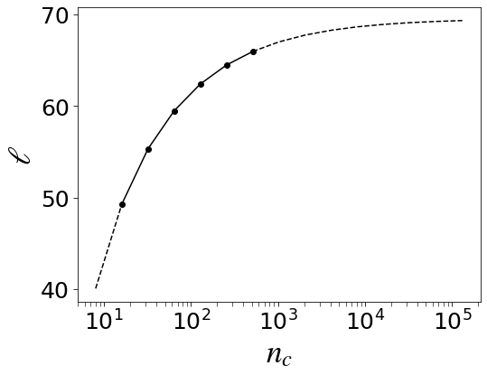
Figure S.1: $n_{\rm c}$ dependence of $\ell$ expressed by (S.73). The solid line shows the range of values we used in our numerical calculations.

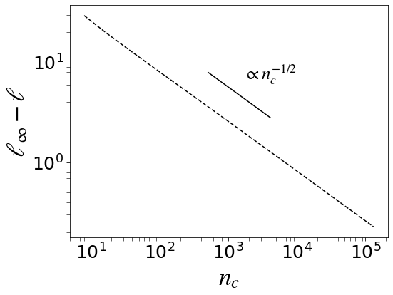
Figure S.2: Asymptotic behavior of $\ell$ converging to $\ell_{\infty}$ given in (S.74). The relation $\ell_{\infty}-\ell=80n_{c}^{-1/2}$ holds for large $n_{c}$.

We first consider the Fourier expansion

$$\int_{0}^{\infty}dt\ C(x,t)=\frac{1}{L}\sum_{n=-n_{\rm c}}^{n_{\rm c}}C_{n}e^{-ik_{n}x}$$ (S.68)

with $k_{n}=2\pi n/L$, where the cut-off number $n_{\rm c}$ is given by $L/(2\Delta x)$. From (S.66), we may set

$$C_{n}=c\left(\frac{D}{\nu\lambda^{2}}\right)^{1/2}k_{n}^{-3/2}$$ (S.69)

for sufficiently large $L$. We then find

$$\int_{0}^{\infty}dt\ \left[C\left(\frac{L}{2},t\right)-C(0,t)\right]$$

$$= \frac{c}{L}\left(\frac{D}{\nu\lambda^{2}}\right)^{1/2}\sum_{n=-n_{\rm c}}^{n_{\rm c}}((-1)^{n}-1)\frac{1}{k_{n}^{3/2}}$$

$$= -\frac{4c}{L}\left(\frac{L}{2\pi}\right)^{3/2}\left(\frac{D}{\nu\lambda^{2}}\right)^{1/2}\sum_{n=1}^{n_{\rm c}/2}\frac{1}{(2n-1)^{3/2}}.$$ (S.70)

Substituting this result into the formula (15) in the main text, we obtain the form

$$\kappa_{\rm eff}=\kappa\left(\frac{L}{L_{0}}\right)^{1/2},$$ (S.71)

where $L_{0}$ is calculated as

$$L_{0}=\ell\frac{\nu^{3}}{D\lambda^{2}}$$ (S.72)

with

$$\ell=\frac{(32c)^{2}}{(2\pi)^{3}}\left(\sum_{n=1}^{n_{\rm c}/2}\frac{1}{(2n-1)^{3/2}}\right)^{2}.$$ (S.73)

This gives the estimation of the dimensionless cross-over length $\ell$ defined by (16) and (18) in the main text.

In Fig. S.2, we plot $\ell$ for $n_{\rm c}$. In the range we studied in numerical simulations, the theoretical estimation of $\ell$ is consistent with the numerically obtained value $\ell\simeq 60$. If we study the case that $L\to\infty$, $\ell$ should be evaluated in the limit $n_{\rm c}\to\infty$. This value, which is denoted by $\ell_{\infty}$, is calculated as

$$\begin{split}\ell_{\infty}&=\frac{(32c)^{2}}{(2\pi)^{3}}\left(\sum_{n=1}^{\infty}\frac{1}{n^{\frac{3}{2}}}-\sum_{n=1}^{\infty}\frac{1}{(2n)^{\frac{3}{2}}}\right)^{2}\\ &=\frac{(32c)^{2}}{(2\pi)^{3}}\left(1-\frac{1}{2^{\frac{3}{2}}}\right)^{2}\zeta\left(\frac{3}{2}\right)^{2}\\ &\simeq 69.52.\end{split}$$ (S.74)

Note that the convergence is slow and Fig. S.2 shows that

$$\ell_{\infty}-\ell(n_{\rm c})=\frac{A}{\sqrt{n_{\rm c}}}$$ (S.75)

for large $n_{\rm c}$, where $A=80$.

III Supplemental data

III.1 Measurement of the response

Figure S.3: Amplitude of the averaged height function against the strength of the external stress for system sizes $L=2,4,8,16,32$, and $64$, from bottom to top. $v_{0}=5$. The symbols show the numerical results and they are fitted to a quadratic function $f_{2}=c_{1}\tilde{\epsilon}+c_{2}\tilde{\epsilon}^{2}$ (solid lines).

Figure S.4: $\kappa_{\rm eff}$ calculated by (S.76) are displayed as a function of $L$. $v_{0}=5$. This shows the divergent behavior $\kappa_{\rm eff}=0.665\sqrt{L}.$

In Fig. 3 of the main text, we display the numerical data of $\left<h(L/2)-h(0)\right>_{\rm ss}^{\epsilon}/\tilde{\epsilon}$. Here, we explain the method for numerically evaluating it. In Fig. S.4, we show $\left<h(0)-h(L/2)\right>_{{\rm ss}}^{\epsilon}$ for several values of $\tilde{\epsilon}$ ranged from $0.002$ to $0.01$ for systems with sizes $L=2,4,8,16,32$, and $64$. For each $L$, we fit the data points by a quadratic function $f_{2}(\tilde{\epsilon})=c_{1}\tilde{\epsilon}+c_{2}\tilde{\epsilon}^{2}$ by the least-square method. This linear coefficient $c_{1}$ is given as $\left\langle h(L/2)-h(0)\right\rangle^{\epsilon}_{\rm ss}/\tilde{\epsilon}$ in Fig. 3 of the main text.

Using the coefficient $c_{1}$ and (7) in the main text, we have

$$\kappa_{{\rm eff}}=\frac{L}{8c_{1}}.$$ (S.76)

Then, we display $\kappa_{{\rm eff}}$ as a function of $L$ in Fig. S.4. This graph already shows the $\sqrt{L}$ behavior of $\kappa_{{\rm eff}}$. However, it is hard to study larger systems than $L=64$ by this method.

III.2 Dynamical-scaling exponent

It has been known that the dynamical exponent $z$ is equal to $3/2$ for the KPZ equation. We directly confirm this fact by numerical simulations. Concretely, we study the height width

$$W(L,t)\equiv\sqrt{\left<(h-\left<h\right>)^{2}\right>}$$ (S.77)

for the initial condition $h(x,0)=0$. In Fig. S.6, we plot $W/L^{1/2}$ against $t/L^{3/2}$ for system sizes $L=64,256,1024,$ and $4096$ with $\nu=D=1$ and $\lambda=5$ fixed. It is found that all the data are on the same universal curve. The scaling function observed in the simulation is consistent with known results.

We note that the same procedure does not yield a clear curve for the numerical simulations of the system with $\lambda=1$, as shown in Fig. S.6. This is interpreted as a finite time effect. Concretely, in the early stage $t\ll t_{0}$, the growth of $W$ is described by the linear (equilibrium) dynamics with $\lambda=0$, while the non-linear growth effect becomes dominant for the late stage $t\gg t_{0}$. The cross-over time $t_{0}$ was numerically obtained [6, 5, 4] as

$$t_{0}\simeq 252\nu^{5}D^{-2}\lambda^{-4}.$$ (S.78)

We conjecture that the cross-over time $t_{0}$ is related to the cross-over length $L_{0}$ in our study.

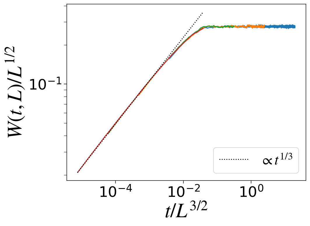
Figure S.5: Dynamical scaling of the width $W$ for the KPZ interface with $\lambda=5$. The system sizes are $L=64,256,1024$, and $4096$ from right to left. The dotted line is a guide to the eye.

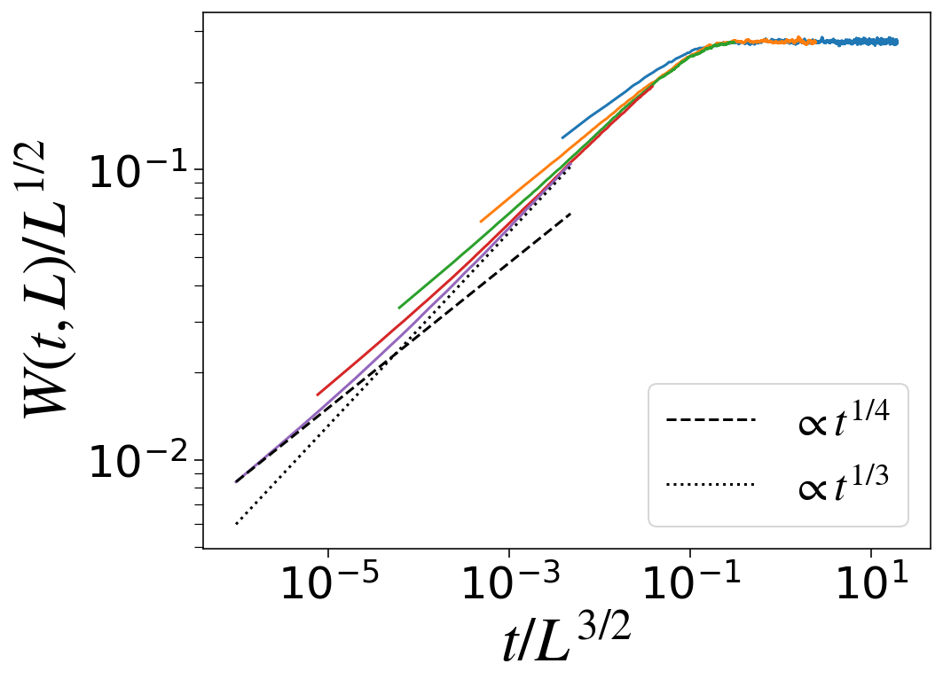
Figure S.6: The same as Fig. S.6, but for $\lambda=1$. The system sizes are $L=64,256,1024,4096$, and $16384$ from right to left. In this case, the width grows as $t^{1/4}$ (dashed line), not $t^{1/3}$ (dotted line), until non-linearity grows enough.

III.3 Finite mesh effect for $\kappa_{\rm eff}(L)$

Since we fix $\Delta x=0.5$ in the discrete model, the model with small $L$ may not provide a good approximation of the KPZ equation. In order to study this aspect more quantitatively, in Fig. S.8, we plot $\kappa_{\rm eff}$ against $L\geq 2$ with $v_{0}=5$ fixed. It shows that $\kappa_{\rm eff}$ is almost proportional to $\sqrt{L}$ for $L\geq 4$. However, when we plot $\kappa_{\rm eff}$ for several values of $v_{0}$ in Fig. S.8, we find that the data for $L=2,4,$ and $8$ are not on the one universal curve. This means that the discrete model with $\Delta x=0.5$ is not a good approximation of the KPZ equation with $L=2,4,$ and $8$. More quantitatively, we notice that the cut-off number $n_{c}=L/(2\Delta x)$ characterizes the cross-over length as shown in (S.73) and Fig. S.2. This means that the system with smaller $n_{c}$ shows a shorter cross-over length, which makes the data points shift to the right side. Therefore, the data for the systems with small $L$ are obviously contaminated by discretization effects and thus deviate from the universal curve determined in the larger systems. For this reason, we employ the data for $L\geq 16$ in the main text.

Figure S.7: $\kappa_{\rm eff}$ for $L=2,4,8,16,32,64,128,256$, and $512$ from left to right. $v_{0}=5$. The symbols $L\geq 4$ are on the straight line corresponding to $\kappa_{\rm eff}=0.646\sqrt{L}$.

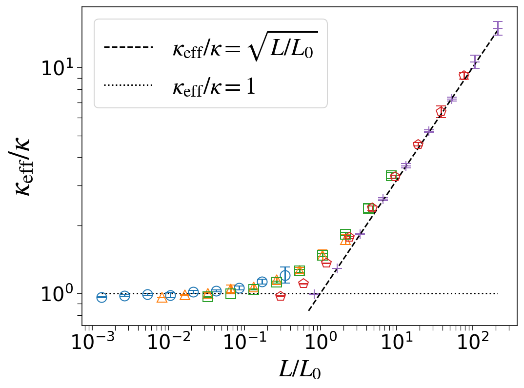
Figure S.8: $\kappa_{\rm eff}$ for the same system sizes as Fig. S.8 and with $v_{0}=0.2,0.5,1,3$, and $5$ (difference in symbols represents the difference in $v_{0}$). $L_{0}$ is given by (S.72) with $\ell\simeq 60$ in this figure. The symbols for the small system sizes $L=2,4$, and $8$ are not in the universal curve.

References

[1]
F. Jülicher, S. W. Grill, and G. Salbreux, Hydrodynamic theory of active matter, Rep. Prog. Phys. 81, 076601 (2018).
[2]
K. A. Takeuchi, An appetizer to modern developments on the Kardar–Parisi–Zhang universality class, Physica A 504, 77 (2018).
[3]
J. Eisert, M. Friesdorf, and C. Gogolin, Quantum many-body systems out of equilibrium, Nature Physics 11, 124 (2015).
[4]
P. C. Hohenberg, Existence of long-range order in one and two dimensions, Phys. Rev. 158, 383 (1967).
[5]
N. D. Mermin and H. Wagner, Absence of ferromagnetism or antiferromagnetism in one- or two-dimensional isotropic Heisenberg models, Phys. Rev. Lett. 17, 1133 (1966).
[6]
J. Toner and Y. Tu, Long-range order in a two-dimensional dynamical XY model: How birds fly together, Phys. Rev. Lett. 75, 4326 (1995).
[7]
H. Nakano, Y. Minami, and S.-i. Sasa, Long-range phase order in two dimensions under shear flow, Phys. Rev. Lett. 126, 160604 (2021).
[8]
T. Harada and S.-i. Sasa, Equality Connecting Energy
Dissipation with a Violation of the Fluctuation-Response
Relation, Phys. Rev. Lett. 95, 130602 (2005).
[9]
T. Speck and U. Seifert,
Restoring a FluctuationDissipation Theorem in a Nonequilibrium Steady State,
Europhys. Lett. 74, 391 (2006).
[10]
R. Chetrite, G. Falkovich, and K. Gawedzki, Fluctuation relations in simple examples of nonequilibrium steady states, J. Stat. Mech. 2008, P08005 (2008).
[11]
M. Baiesi, C. Maes and B. Wynants, Fluctuations and response of nonequilibrium states, Phys. Rev. Lett 103, 010602 (2009).
[12]
J. Prost, J.-F. Joanny and J. M. R. Parrondo, Generalized fluctuation-dissipation theorem for steady-state systems, Phys. Rev. Lett. 103, 090601 (2009).
[13]
M. Baiesi and C. Maes,
An update on the nonequilibrium linear response,
New J. Phys. 15, 013004 (2013).
[14]
V. Blickle, T. Speck, C. Lutz, U. Seifert, and C. Bechinger, Einstein Relation Generalized to Nonequilibrium, Phys. Rev. Lett. 98, 210601 (2007).
[15]
J. R. Gomez-Solano, A. Petrosyan, S. Ciliberto, R. Chetrite, and K. Gawedski,
Experimental Verification of a Modified Fluctuation-Dissipation Relation
for a Micron Sized Particle in a Nonequilibrium Steady State,
Phys. Rev. Lett. 103, 040601 (2009).
[16]
S. Toyabe, T. Okamoto, T. W. Nakayama, H. Taketani, S. Kudo, and E. Muneyuki,
Nonequilibrium Energetics of a Single F1-ATPase Molecule,
Phys. Rev. Lett. 104, 198103 (2010).
[17]
J. A. Mclennan, Statistical mechanics of transport in fluids, Phys. Fluids 3, 493 (1960).
[18]
D. N. Zubarev, Nonequilibrium Statistical Thermodynamics, (Consultants Bureau, New York, 1974)
[19]
R. Kubo, M. Toda, and N. Hashitsume, Statistical Physics II: Nonequilibrium Statistical Mechanics, (Springer-Verlag, Berlin, Germany, 1991)
[20]
S. F. Edwards and D. R. Wilkinson, The surface statistics of a granular aggregate, Proc. R. Soc. Lond. A 381, 17 (1982).
[21]
M. Kardar, G. Parisi, and Y. Zhang, Dynamic scaling of growing interfaces, Phys. Rev. Lett. 56, 889 (1986).
[22]
A. Dhar, Heat transport in low-dimensional systems, advances in physics 57, 457 (2008).
[23]
D. Forster, D. R. Nelson, and M. J. Stephen, Large-distance and long-time properties of a randomly stirred fluid, Phys. Rev. A 16, 732 (1977).
[24]
S. Lepri (Ed.), Thermal Transport in Low Dimensions. From Statistical Physics to Nanoscale Heat Transfer, (Springer International Publishing, Cham, Switzerland, 2016)
[25]
See Supplemental Material at [URL will be inserted by publisher] for derivations and detailed explanations.
[26]
K. A. Takeuchi, M. Sano, Evidence for geometry-dependent universal fluctuations of the Kardar-Parisi-Zhang interfaces in liquid-crystal turbulence, J. Stat. Phys. 147, 853 (2012).
[27]
J. Maunuksela, M. Myllys, O.-P. Kähkönen, J. Timonen, N. Provatas, M. J. Alava, and T. Ala-Nissila, Kinetic Roughening in Slow Combustion of Paper, Phys. Rev. Lett. 79, 1515 (1997)
[28]
J.-i. Wakita, H. Itoh, T. Matsuyama, M. Matsushita, Self-affinity for the growing interface of bacterial colonies, J. Phys. Soc. Jpn. 66, 67 (1997).
[29]
T. Halpin-Healy and K. A. Takeuchi, A KPZ Cocktail- shaken, not stirred: toasting 30 years of kinetically roughened surfaces, J. Stat. Phys. 160, 794 (2015).
[30]
P. Meakin, The growth of rough surfaces and interfaces, Physics Reports 235, 189 (1993).
[31]
T. J. Newman and A. J. Bray, Strong-coupling behaviour in discrete Kardar - Parisi - Zhang equations, J. Phys. A: Math. Gen. 29, 7917 (1996).
[32]
C. Lam and F. G. Shin, Improved discretization of the Kardar-Parisi-Zhang equation, Phys. Rev. E 58, 5592 (1998).
[33]
V. G. Miranda and F. D. A. A. Reis, Numerical study of the Kardar-Parisi-Zhang equation, Phys. Rev. E 77, 031134 (2008)
[34]
H. S. Wio, J. A. Revelli, R. R. Deza, C. Escudero, and M. S. de La Lama, Discretization-related issues in the Kardar-Parisi-Zhang equation: Consistency, Galilean-invariance violation, and fluctuation-dissipation relation, Phys. Rev. E 81, 066706 (2010)
[35]
M. Dentz, I. Neuweiler, Y. Méheust, and D. M. Tartakovsky, Noise-driven interfaces and their macroscopic representation, Phys. Rev. E 94, 052802 (2016).
[36]
Priyanka, U. C. Täuber, and M. Pleimling, Feedback control of surface roughness in a one-dimensional Kardar-Parisi-Zhang growth process, Phys. Rev. E 101, 022101 (2020).
[37]
H. van Beijeren, R. Kutner, and H. Spohn, Excess noise for driven diffusive systems, Phys. Rev. Lett. 54, 2026 (1985).
[38]
E. Medina, T. Hwa, M. Kardar, and Y. Zhang, Burgers equation with correlated noise: Renormalization-group analysis and applications to directed polymers and interface growth, Phys. Rev. A 39, 3053 (1989).
[39]
E. Frey and U. C. Täuber, Two-loop renormalization-group analysis of the Burgers–Kardar-Parisi-Zhang equation, Phys. Rev. E 50, 1024 (1994).
[40]
F. Colaiori and M. A. Moore, Numerical solution of the mode-coupling equations for the Kardar-Parisi-Zhang equation in one dimension, Phys. Rev. E 65, 017105 (2001).
[41]
M. Prähofer and H. Spohn, Exact scaling functions for one-dimensional stationary KPZ growth, J. Stat. Phys. 115, 255 (2004).
[42]
L. Canet, H. Chaté, B. Delamotte, and N. Wschebor, Nonperturbative renormalization group for the Kardar-Parisi-Zhang equation: General framework and first applications, Phys. Rev. E 84, 061128 (2011).
[43]
O. Niggemann and U. Seifert, The two scaling regimes of the thermodynamic uncertainty relation for the KPZ-equation, J. Stat. Phys. 186, 1 (2022).
[44]
T. Sasamoto and H. Spohn, One-dimensional Kardar-Parisi-Zhang equation: An exact solution and its universality, Phys. Rev. Lett. 104, 230602 (2010).
[45]
V. Dotsenko, Bethe ansatz derivation of the Tracy-Widom distribution for one-dimensional directed polymers, Europhys. Lett. 90, 20003 (2010).
[46]
P. Calabrese, P. L. Doussal, and A. Rosso, Free-energy distribution of the directed polymer at high temperature, Europhys. Lett. 90, 20002 (2010).
[47]
G. Amir, I. Corwin, and J. Quastel, Probability distribution of the free energy of the continuum directed random polymer in 1 + 1 dimensions, Communications on Pure and Applied Mathematics 64, 466 (2011).
[48]
T. Kloss, L. Canet, and N. Wschebor, Nonperturbative renormalization group for the stationary Kardar-Parisi-Zhang equation: Scaling functions and amplitude ratios in 1+1, 2+1, and 3+1 dimensions, Phys. Rev. E 86, 051124 (2012).
[49]
T. Imamura and T. Sasamoto, Stationary correlations for the 1D KPZ equation, J. Stat. Phys. 150, 908 (2013).
[50]
M. Hairer, Solving the KPZ equation, Annals of Mathematics 178, 559 (2013).
[51]
K. Johansson, The two-time distribution in geometric last-passage percolation, Probab. Theory Relat. Fields 175, 849 (2019).
[52]
D. J. Evans, E. G. D. Cohen, and G. P. Morriss, Probability of second law violations in shearing steady states, Phys. Rev. Lett. 71, 2401 (1993).
[53]
G. Gallavotti and E. G. D. Cohen, Dynamical ensembles in nonequilibrium statistical mechanics, Phys. Rev. Lett. 74, 2694 (1995).
[54]
J. Kurchan, Fluctuation theorem for stochastic dynamics,
J. Phys. A: Math. Gen.
31, 3719 (1998).
[55] U. Seifert,
Stochastic thermodynamics, fluctuation theorems
and molecular machines, Rep. Prog. Phys. 75, 126001 (2012).
[56]
S.-i. Sasa, A fluctuation theorem for phase turbulence of chemical oscillatory waves, arXiv:nlin/0010026 (2000).
[57]
P. C. Martin, E. D. Siggia, and H. A. Rose, Statistical dynamics of classical systems, Phys. Rev. A 8, 423 (1973).
[58]
U. Deker and F. Haake, Fluctuation-dissipation theorems for classical processes, Phys. Rev. A 11, 2043 (1975).
[59]
H. Janssen, On a Lagrangean for classical field dynamics and renormalization group calculations of dynamical critical properties, Z. Phys. B 23, 377 (1976).
[60]
K. A. Takeuchi, Experimental approaches to universal out-of-equilibrium scaling laws: turbulent liquid crystal and other developments, J. Stat. Mech. 2014, P01006 (2014).