Asymptotical Cooperative Cruise Fault Tolerant Control for Multiple High-speed Trains with State Constraints

Abstract

This paper investigates the asymptotical cooperative cruise fault tolerant control problem for multiple high-speed trains consisting of multiple carriages in the presence of actuator faults. A distributed state-fault observer utilizing the structural information of faults is designed to achieve asymptotical estimation of states and faults of each carriage. The observer does not rely on choice of control input, and thus it is separated from controller design. Based on the estimated values of states and faults, a distributed fault tolerance controller is designed to realize asymptotical cooperative cruise control of trains under the dual constraints of ensuring both position difference and velocity difference of adjacent trains in specified ranges throughout the whole process.

1 Introduction

High-speed trains (HSTs) have become an increasingly popular mode of travel worldwide due to their efficiency, reliability, and comfort; Di Meo et al. (2019), Li et al. (2020), Cascetta et al. (2020). Shortening train tracking interval to improve the existing railway utilization efficiency is an efficient and economic method to relieve the pressure of passenger transport. It was reported in Dong et al. (2016); Schumann (2017); Song and Schnieder (2018); Felez et al. (2019); Cao et al. (2021) that cooperative cruise control can realize synchronous operation of a large number of trains in a very short tracking distance, which is of great significance for improving railway utilization efficiency.

The train-to-train (T2T) wireless communication technology was developed for HSTs in such as Jikang et al. (2017); Unterhuber et al. (2018); Song and Schnieder (2019); Wang et al. (2019); Zhu et al. (2022), as shown in Fig. 1. The global system for mobile communication-railway (GSM-R) network is responsible for bidirectional real-time information transmission between on-board equipment and the radio block center (RBC). This technology offers direct communication between adjacent trains and facilitates cooperative cruise control of trains.

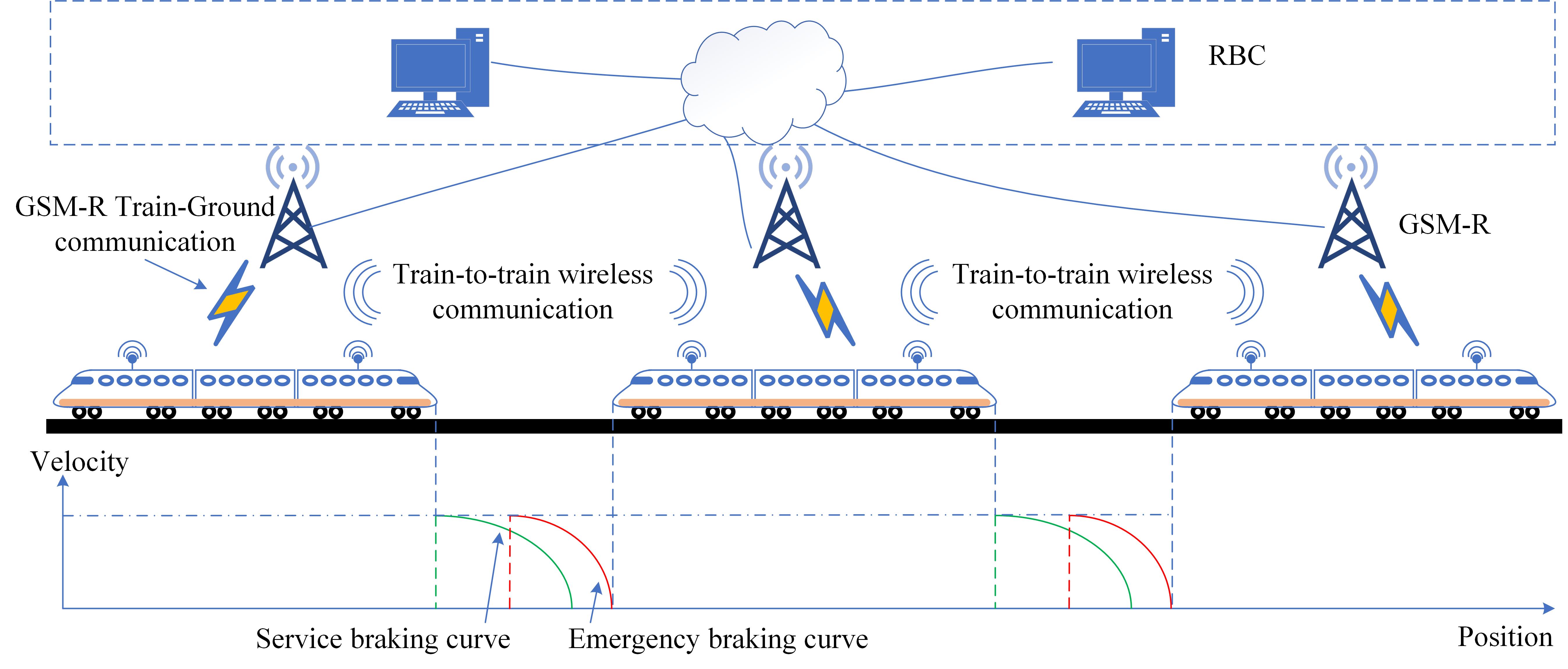
Figure 1: Schematic diagram of cooperative operation of trains based on T2T wireless communication

A cooperative cruise control scheme has two tasks. On one hand, cruise control of a train aims to adjust the real-time velocity to track a reference velocity profile that is specified based on different performance indexes such as energy consumption, comfort, and time consumption; see Wang et al. (2013); Goverde et al. (2016). On the other hand, cooperative control of trains means that each train designs its controller based on the real-time information transmitted by neighboring trains, and eventually achieves the same velocity on the premise of ensuring safe operation of all trains; see Dong et al. (2016); Wang et al. (2019); Li and Duan (2017).

Cooperative cruise control of trains has attracted wide attention in recent years. The state-of-the-art research in this area is discussed from different perspectives below. For instance, a single-particle train model was studied in Li et al. (2015); Gao et al. (2018); Bai et al. (2020); Dong et al. (2016); Bai et al. (2021a, b), where the train is regarded as a rigid body and the torques between adjacent carriages are ignored. A more accurate multiple-particle model treats every carriage as a mass point and considers the torque between carriages, which makes the design of the controller more flexible and realistic.

In most references such as Li et al. (2015); Gao et al. (2018); Wang et al. (2019); Bai et al. (2020); Dong et al. (2016); Zhao et al. (2017), the train model is a second-order position-velocity model, which ignores the dynamic response from the designed input voltage of a motor to the real output torque, under an ideal assumption that the motor servo system is zero order. In practice, design of an ideal motor servo system is costly. Therefore, it is of interest to study a more realistic model composed of a second-order position-velocity model and a dynamics motor servo system (treated as a first-order model), which results in a third-order position-velocity-acceleration model. Some relevant work can be found in Bai et al. (2021a, b).

It is a critical safety requirement to constrain the position spacing of trains in dynamic operation, as studied in literature such as Li et al. (2015); Bai et al. (2020); Wang et al. (2019); Zhao et al. (2017). While these works only consider position constraint, trains can be constrained at both the position and velocity levels to further improve the safety of operation.

Lastly, fault tolerance is critical for the cooperative cruise control scheme as potential actuator faults may threaten stable operation of trains and even cause serious accidents. There has been a lot of research on fault tolerance control of individual HSTs. For example, in Mao et al. (2017), an adaptive law was designed to update the parameters of the adaptive controller, so as to realize fault compensation of HSTs under the condition that the system piecewise constant parameters and the actuator failure parameters are unknown. In Yao et al. (2018), two Markov chains model were used to describe the failure process and the failure detection and identification process of HSTs respectively, and an active fault tolerant composite hierarchical anti-disturbance control strategy based on a disturbance observer was proposed.

In Zhu et al. (2022), a distributed fault-tolerant control strategy was proposed to deal with the cooperative control problem of HSTs with actuator faults. However, the control strategy is aimed at the second-order single-particle train model, and does not consider the safety constraint of the distance between trains when multiple trains operate cooperatively, which brings safety hazards to short-distance tracking operation. Furthermore, there are few researches on cooperative control of the third-order train model with actuator faults. To the best of our knowledge, the research on fault tolerance control of the third-order train model was limited to the problem of a single train in Song et al. (2013).

Most studies on fault-tolerant control assume that the fault model is unknown but additional bounded constraints or other conditions need to be added. These methods always lead to bounded error of fault estimation and thus bounded error of fault tolerance control; see Ge et al. (2019); Mao et al. (2019); Lin et al. (2018); Yao et al. (2018); Zhu et al. (2022). However, actual train actuator faults are mainly constant faults and periodic faults as seen in Mao et al. (2019); Liu et al. (2019). By utilizing such structural information, a fault estimation observer was proposed in Zhang and Chen (2022) for a class of second-order systems, and a fault tolerance controller was designed based on the observed states to achieve asymptotic tracking. The approach is further developed in this paper for a third-order system and applied to HSTs to realize cooperative cruise fault-tolerant control.

The main contributions are summarized as follows.

• A class of third-order multi-particle model of multiple HSTs with actuator faults is established. The fault is described based on a new representation, which contains the structural information and is of great significance for the asymptotical estimation.

• A distributed state-fault observer is designed for every carriage of every train, which can realize asymptotical estimation of states and faults. The observer does not rely on the control input, which separates designs of observer and controller and provides great convenience in theoretical analysis.

• A distributed cooperative cruise fault-tolerant controller is designed for all carriages of all trains. All carriages of each train can asymptotically track the velocity profile of the head carriage, and the position difference between every adjacent carriages of a same train converges to the nominal value. Also, the position difference and velocity difference of adjacent trains are constrained within the specified range throughout the whole process, the velocity of every train aymptotically tracks the reference velocity, and the distance between adjacent trains eventually converges to the prescribed distance.

The rest of this paper is organized as follows. The dynamic model and the control objective are given in Section 2. Section 3 presents the design of a state-fault observer. In Section 4, a cooperative cruise fault tolerance controller is explicitly developed. The numerical simulation results are presented in Section 5. Finally, Section 6 concludes this paper.

2 Problem Formulation and Preliminaries

2.1 Modeling

Consider a railway network system of $N\geq 1$ trains, labelled as $i=1,\cdots,N$, each of which is composed of $M_{i}\geq 1$ carriages, labelled as $j=1,\cdots,M_{i}$. Denote the sets of trains and carriages as

$${\mathbb{T}}= \{i\;|\;i=1,\cdots,N\},$$

$${\mathbb{C}}= \{(i,j)\;|\;j=1,\cdots,M_{i},\;i\in{\mathbb{T}}\},$$

respectively. Also, denote the sets of head carriages and other (non-head) carriages as

$${\mathbb{C}}_{h}= \{(i,j)\ |\ j=1,\;i\in{\mathbb{T}}\},$$

$${\mathbb{C}}_{o}= \{(i,j)\ |\ j=2,\cdots,M_{i},\;i\in{\mathbb{T}}\},$$

respectively. One has ${\mathbb{C}}={\mathbb{C}}_{h}\cup{\mathbb{C}}_{o}$.

The dynamics of each carriage are described as follows:

$$\dot{x}_{ij}= v_{ij}$$

$$\dot{v}_{ij}= \frac{1}{m_{ij}}(\tau_{ij}-B_{ij}(x_{i},v_{i})-m_{ij}R(v_{ij})),\;(i,j)\in{\mathbb{C}},$$ (1)

where $x_{ij}$, $v_{ij}$, and $\tau_{ij}$ are the position, the velocity, and the input representing the traction/braking force, respectively. The mass of carriage is $m_{ij}$, the function $R(v_{ij})$ characterizes the aerodynamic drag and rolling mechanical resistance, and the term $B_{ij}(x_{i},v_{i})$, with the lumped vectors $x_{i}=[x_{i1},\cdots,x_{i,M_{i}}]^{T}$ and $v_{i}=[v_{i1},\cdots,v_{i,M_{i}}]^{T}$, represents the coupling force caused by the adjacent carriage(s). Specifically,

$$R(v_{ij})=c_{0}+c_{1}v_{ij}+c_{2}v_{ij}^{2},$$

where $c_{0}$, $c_{1}$ and $c_{2}$ are the Davis formula coefficients; and

$$B_{ij}(x_{i},v_{i})=\begin{cases}&a(x_{i1}-x_{i2}-d_{p})+b(v_{i1}-v_{i2}),\ j=1\vspace{2mm}\\ &a(2x_{ij}-x_{i(j-1)}-x_{i(j+1)})+b(2v_{ij}\\ &-v_{i(j-1)}-v_{i(j+1)}),\ j=2,\cdots,M_{i}-1\vspace{2mm}\\ &a(x_{iM_{i}}-x_{i(M_{i}-1)}+d_{p})+b(v_{iM_{i}}\\ &-v_{i(M_{i}-1)}),\ j=M_{i}\end{cases},$$

where $d_{p}$, $a$ and $b$ are the nominal length (including the length of a carriage), the stiffness coefficient and the damping constant of carriage couplers, respectively.

Assume the dynamic response of the actuator for generating $\tau_{ij}$ is characterized by the following first-order differential equation

$$\dot{\tau}_{ij}=-r_{ij}\tau_{ij}+\varpi_{ij}+E_{ij}f_{ij},\;(i,j)\in{\mathbb{C}}$$ (2)

where $\varpi_{ij}$ is the desired force to be designed, $r_{ij}$ is the time constant, and $E_{ij}f_{ij}$ represents the fault that may occur in the actuator. The servomechanism for generating such closed-loop regulation performance is out of the scope of this paper.

Assume the fault $f_{ij}$ has the model

$$\dot{f}_{ij}= S_{ij}f_{ij},\;(i,j)\in{\mathbb{C}}$$ (3)

for a constant matrix $S_{ij}$. Train actuator faults are typically constant faults and periodic faults as studied in Mao et al. (2019); Liu et al. (2019). They can be well accommodated by the model (3). It is worth mentioning that most of the existing works neglect the fault model, which leads to residual fault estimation errors and thus affects accuracy of fault tolerance control. In this paper, a reasonable model is established for the common constant fault and periodic fault, and the fault model information is effectively exploited, which is beneficial to asymptotical estimation of the faults and improvement of control accuracy.

Example 2.1

Consider the fault $f_{ij}$ of the model (3) with

$$f_{ij}=\begin{bmatrix}f_{ij1}\\ f_{ij2}\\ f_{ij3}\end{bmatrix},\;S_{ij}=\begin{bmatrix}0&0&0\\ 0&0&\omega_{ij}\\ 0&-\omega_{ij}&0\end{bmatrix}.$$

Then, the fault $f_{ij}$ contains a constant mode and a sinusoidal model of frequency $\omega_{ij}$. In particular, if we select $E_{ij}=\begin{bmatrix}\upsilon_{ij}&0&\nu_{ij}\omega_{ij}\end{bmatrix}$, the fault in (2) is

$$E_{ij}f_{ij}=\upsilon_{ij}f_{ij1}+\nu_{ij}\omega_{ij}f_{ij3}.$$

Assume the faults occur in certain periods, one has

$$f_{ij1}(t)= \left\{\begin{array}[]{ll}{F_{cij}},&t\in[t^{s}_{ij1},t^{e}_{ij1}]\\ 0,&\text{otherwise}\end{array}\right.$$

$$f_{ij3}(t)= \left\{\begin{array}[]{ll}{F_{pij}}\cos(\omega_{ij}t+{F_{\phi ij}}),&t\in[t^{s}_{ij3},t^{e}_{ij3}]\\ 0,&\text{otherwise}\end{array}\right.$$

for some unknown parameters ${F_{cij}}$, ${F_{pij}}$, ${F_{\phi ij}}$.

2.2 Preliminary Manipulation

Let $w_{ij}:=\dot{v}_{ij}$ be the acceleration of the carriage $(i,j)$, which is not measurable in the present setting due to practical restriction. Taking $w_{ij}$ as a new state, we can calculate $\dot{w}_{ij}=\ddot{v}_{ij}$ as follows,

$$\dot{w}_{ij}= -\frac{r_{ij}}{m_{ij}}\tau_{ij}+\frac{\varpi_{ij}}{m_{ij}}+\frac{E_{ij}}{m_{ij}}f_{ij}$$

$$-\frac{1}{m_{ij}}\frac{dB_{ij}(x_{i},v_{i})}{dt}-\frac{\partial R(v_{ij})}{\partial v_{ij}}\dot{v}_{ij}$$

$$= -r_{ij}w_{ij}-\frac{r_{ij}}{m_{ij}}B_{ij}(x_{i},v_{i})-r_{ij}R(v_{ij})+\frac{\varpi_{ij}}{m_{ij}}$$

$$+C_{ij}f_{ij}-\frac{1}{m_{ij}}\frac{dB_{ij}(x_{i},v_{i})}{dt}-\frac{\partial R(v_{ij})}{\partial v_{ij}}w_{ij}$$

$$= -\frac{r_{ij}}{m_{ij}}B_{ij}(x_{i},v_{i})-r_{ij}R(v_{ij})+\frac{\varpi_{ij}}{m_{ij}}+C_{ij}f_{ij}$$

$$+B^{1}_{ij}(v_{ij})w_{ij}+B^{2}_{ij}w_{i(j-1)}+B^{3}_{ij}w_{i(j+1)}+B^{4}_{ij}(v_{i})$$ (4)

where $\tau_{ij}=m_{ij}w_{ij}+B_{ij}(x_{i},v_{i})+m_{ij}R(v_{ij})$, by (1), is used, and the quantities are defined as follows,

$$C_{ij}=E_{ij}/m_{ij}$$

$$B^{1}_{ij}(v_{ij})=\left\{\begin{array}[]{l}-\frac{b}{m_{ij}}-(c_{1}+2c_{2}v_{ij})-r_{ij},\ j=1,M_{i}\\ -\frac{2b}{m_{ij}}-(c_{1}+2c_{2}v_{ij})-r_{ij},\ j=2,\cdots,M_{i}-1\end{array}\right.$$

$$B^{2}_{ij}=\left\{\begin{array}[]{l}0,\ j=1\\ \frac{b}{m_{ij}},\ j=2,\cdots,M_{i}\end{array}\right.$$

$$B^{3}_{ij}=\left\{\begin{array}[]{l}\frac{b}{m_{ij}},\ j=1,\cdots,M_{i}-1\\ 0,\ j=M_{i}\end{array}\right.$$

$$B^{4}_{ij}(v_{i})=\left\{\begin{array}[]{l}-\frac{a(v_{i1}-v_{i2})}{m_{ij}},\ j=1\\ -\frac{a(2v_{ij}-v_{i(j-1)}-v_{i(j+1)})}{m_{ij}},\ j=2,\cdots,M_{i}-1\\ -\frac{a(v_{iM_{i}}-v_{i(M_{i}-1)})}{m_{ij}},\ j=M_{i}\end{array}\right..$$

The preliminary controller $\varpi_{ij}$ in (2) is constructed as follows,

$$\varpi_{ij}= m_{ij}u_{ij}+r_{ij}B_{ij}(x_{i},v_{i})+m_{ij}r_{ij}R(v_{ij})$$

$$-m_{ij}B^{4}_{ij}(v_{i}),\;(i,j)\in{\mathbb{C}},$$ (5)

where $u_{ij}$ is the new input to be designed.

From the above manipulation, the system composed of (1), (2), (3), (4), and (5) is equivalent to the following composite model

$$\dot{x}_{ij}= v_{ij}$$

$$\dot{v}_{ij}= w_{ij}$$

$$\dot{w}_{ij}= B^{1}_{ij}(v_{ij})w_{ij}+B^{2}_{ij}w_{i(j-1)}+B^{3}_{ij}w_{i(j+1)}$$

$$+C_{ij}f_{ij}+u_{ij}$$

$$\dot{f}_{ij}= S_{ij}f_{ij},\;(i,j)\in{\mathbb{C}},$$ (6)

which will be studied in the remaining sections of this paper. For the convenience of presentation, the full state of (6) is denoted as $\chi_{ij}=\operatorname{col}(x_{ij},v_{ij},w_{ij},f_{ij})$.

2.3 Objectives

Accurate regulation of trains to a velocity-position profile is of great significance to ensure safe running distance and punctual running time. Let the desired position, velocity, acceleration, and control input be $x_{0}$, $v_{0}$, $w_{0}$, and $u_{0}$ respectively, and they satisfy

$$\dot{x}_{0}=v_{0},\ \dot{v}_{0}=w_{0},\ \dot{w}_{0}=u_{0}.$$ (7)

For the system (6), the objective of this paper is to design $u_{ij}$ such that the closed-loop system satisfies the requirements ${\bf R1}$, ${\bf R2}$, and ${\bf R3}$ defined below.

(i) For each train, the position difference between every adjacent carriages converges to the nominal value $d_{p}$, and the velocity difference converges to zero. Therefore, the first control requirement is

$${\bf R1:}\lim_{t\rightarrow\infty}[x_{i(j-1)}(t)-x_{ij}(t)]= d_{p}$$

$$\lim_{t\rightarrow\infty}[v_{i(j-1)}(t)-v_{ij}(t)]= 0,\;(i,j)\in{\mathbb{C}}_{o}.$$ (8)

(ii) To ensure reliable train-to-train communication, the distance between two adjacent trains must be less than the maximum communication radius $\gamma_{1}>0$. In addition, in order to avoid the risk of collision, the distance must be larger than the emergency braking distance $\gamma_{2}>0$. In order to improve utilization of tracks, it is also a requirement to ensure that the distance is asymptotically maintained at the service braking distance $d_{s}$ satisfying $\gamma_{2}<d_{s}<\gamma_{1}$. Denote $\rho_{1}=\gamma_{1}-d_{s}$ and $\rho_{2}=d_{s}-\gamma_{2}$. Let

$$\tilde{x}_{i}(t)=\epsilon_{i}(t)-d_{s},\;\epsilon_{i}= x_{(i-1)M_{i-1}}-x_{i1},\;i\in{\mathbb{T}}$$ (9)

where $\epsilon_{i}$ is the distance between the $i$-th and $(i-1)$-th trains. Then, the second control requirement is

$${\bf R2:} -\rho_{2}<\tilde{x}_{i}(t)<\rho_{1},\ \forall t\geq 0$$

$$\lim_{t\rightarrow\infty}\tilde{x}_{i}(t)=0,\;i\in{\mathbb{T}}.$$ (10)

It is noted that, ${\bf R2}$ is equivalent to

$$\gamma_{2}<\epsilon_{i}(t)<\gamma_{1},\ \forall t\geq 0$$

$$\lim_{t\rightarrow\infty}\epsilon_{i}(t)=d_{s},\;i\in{\mathbb{T}}.$$

(iii) In order to achieve stable communication between trains and reduce the risk of train collision, it is of great significance to restrict the velocity difference between adjacent trains within the prescribed range $(-\sigma_{2},\sigma_{1})$ and eventually converge to zero, with $\sigma_{1}>0$ and $\sigma_{2}>0$. Define $\tilde{v}_{i}(t)=v_{(i-1)M_{i-1}}-v_{i1}$, then

$${\bf R3:} -\sigma_{2}<\tilde{v}_{i}(t)<\sigma_{1},\ \forall t\geq 0$$

$$\lim_{t\rightarrow\infty}\tilde{v}_{i}(t)=0,\;i\in{\mathbb{T}}.$$ (11)

Remark 2.1

For complement of notation, it is assumed the the $0$-th train is a virtual train whose model is (7) and $x_{(i-1)M_{i-1}}=x_{0}$ and $v_{(i-1)M_{i-1}}=v_{0}$ for $i=1$. Select any $0<\ell_{i1}<\min\{\sigma_{2}/\rho_{1},\sigma_{1}/\rho_{2}\}$. Let $\varrho_{1}=-\ell_{i1}\rho_{2}+\sigma_{1}>0$ and $\varrho_{2}=-\ell_{i1}\rho_{1}+\sigma_{2}>0$. Define a new error combination term $\tilde{q}_{i}(t)=\tilde{v}_{i}(t)+\ell_{i1}\tilde{x}_{i}(t)$ and the associated requirement

$${\bf R3^{\prime}:} -\varrho_{2}<\tilde{q}_{i}(t)<\varrho_{1},\ \forall t\geq 0$$

$$\lim_{t\rightarrow\infty}\tilde{q}_{i}(t)=0,\;i\in{\mathbb{T}}.$$ (12)

When the requirements (10) and (12) are satisfied, so is the requirement (11). Therefore, ${\bf R3}$ can be replaced by ${\bf R3^{\prime}}$.

Remark 2.2

The reference singles $x_{0}$, $v_{0}$, $w_{0}$, and $u_{0}$ in (7) are known for the head carriage of the first train. The state variables $x_{ij}$ and $v_{ij}$ are measurable by means of a speedometer and a milemeter equipped on a train (or other modern advanced technology such as Global Positioning System, Doppler radar, microwave radar, etc.).

3 Observer Design

To address the challenge caused by the existence of unknown faults $f_{ij}$ and unmeasurable states $w_{ij}$, we first design an observer in this section to achieve accurate estimation of $f_{ij}$ and $w_{ij}$, and then design a controller based on the estimated values in the next section to achieve the three control requirements. The observer is designed as follows, with the state $\hat{\chi}_{ij}=\operatorname{col}(\hat{x}_{ij},\hat{v}_{ij},\hat{w}_{ij},\hat{f}_{ij})$,

$$\dot{\hat{x}}_{ij}= \hat{v}_{ij}+\mu_{{ij}1}$$

$$\dot{\hat{v}}_{ij}= \hat{w}_{ij}+\mu_{{ij}2}$$

$$\dot{\hat{w}}_{ij}= B^{1}_{ij}(v_{ij})\hat{w}_{ij}+B^{2}_{ij}\hat{w}_{i(j-1)}$$

$$+B^{3}_{ij}\hat{w}_{i(j+1)}+C_{ij}\hat{f}_{ij}+u_{ij}+\mu_{{ij}3}$$

$$\dot{\hat{f}}_{ij}= S_{ij}\hat{f}_{ij}+\mu_{{ij}4},(i,j)\in{\mathbb{C}}$$ (13)

where $\hat{x}_{ij}$, $\hat{v}_{ij}$, $\hat{w}_{ij}$, and $\hat{f}_{ij}$ are the estimation of $x_{ij}$, $v_{ij}$, $w_{ij}$, and $f_{ij}$, respectively. The auxiliary inputs $\mu_{{ij}1}$, $\mu_{{ij}2}$, $\mu_{{ij}3}$ and $\mu_{{ij}4}$ can be designed as follows.

$$\mu_{{ij}1}= -k_{{ij}1}(\hat{x}_{ij}-x_{ij})+(v_{ij}-\hat{v}_{ij})$$

$$\mu_{ij2}= D^{1}_{ij}(v_{ij})-D^{1}_{ij}(\hat{v}_{ij})+k_{ij2}(\hat{v}_{ij}-v_{ij})$$

$$+D^{2}_{ij}(v_{i(j-1)})-D^{2}_{ij}(\hat{v}_{i(j-1)})$$

$$+D^{3}_{ij}(v_{i(j+1)})-D^{3}_{ij}(\hat{v}_{i(j+1)})$$

$$\mu_{ij3}= B^{1}_{ij}(v_{ij})\mu_{ij2}+k_{ij3}(\hat{v}_{ij}-v_{ij})$$

$$+(B^{1}_{ij}(\hat{v}_{ij})-B^{1}_{ij}(v_{ij}))(\hat{w}_{ij}+\mu_{ij2})$$

$$+B^{2}_{ij}\mu_{i(j-1)2}+B^{3}_{ij}\mu_{i(j+1)2}$$

$$\mu_{ij4}= k_{ij4}(\hat{v}_{ij}-v_{ij})$$ (14)

where

$$D^{1}_{ij}(v_{ij})=\left\{\begin{array}[]{l}-\frac{b}{m_{ij}}v_{ij}-(c_{1}v_{ij}+c_{2}v_{ij}^{2}),\ j=1,M_{i}\\ -\frac{2b}{m_{ij}}v_{ij}-(c_{1}v_{ij}+c_{2}v_{ij}^{2}),\ j=2,\cdots,M_{i}-1\end{array}\right.$$ (17)

$$D^{2}_{ij}(v_{i(j-1)})=\left\{\begin{array}[]{l}0,\ j=1\\ \frac{b}{m_{ij}}v_{i(j-1)},\ j=2,\cdots,M_{i}\end{array}\right.$$ (20)

$$D^{3}_{ij}(v_{i(j+1)})=\left\{\begin{array}[]{l}\frac{b}{m_{ij}}v_{i(j+1)},\ j=1,\cdots,M_{i}-1\\ 0,\ j=M_{i}\end{array}\right..$$ (23)

The main result is stated in the following theorem.

Theorem 1

Consider the system composed of (6) and the observer (13) with the auxiliary inputs designed in (14). The parameters $k_{ij1}>0$ and $K_{ij}=[k_{{ij}2},k_{{ij}3},k_{{ij}4}^{T}]^{T}$ are selected such that the matrix $(A_{ij}+K_{ij}C_{ij})$ is Hurwitz. Then, estimation is asymptotically achieved in the sense of

$$\lim_{t\rightarrow\infty}[\chi_{ij}(t)-\hat{\chi}_{ij}(t)]=0,\;(i,j)\in{\mathbb{C}}.$$ (24)

Let $e_{p{ij}}=\hat{p}_{{ij}}-p_{ij}$, $p\in\{x,v,w,f\}$. The error dynamics can be obtained as follows,

$$\dot{e}_{x{ij}}= e_{v{ij}}+\mu_{{ij}1}$$

$$\dot{e}_{v{ij}}= e_{w{ij}}+\mu_{{ij}2}$$

$$\dot{e}_{w{ij}}= B^{1}_{ij}(v_{ij})e_{w{ij}}+B^{2}_{ij}e_{w{i(j-1)}}$$

$$+B^{3}_{ij}e_{w{i(j+1)}}+C_{ij}e_{f{ij}}+\mu_{{ij}3}$$

$$\dot{e}_{f{ij}}= S_{ij}e_{f{ij}}+\mu_{{ij}4}$$

Let $\zeta_{ij}=e_{w{ij}}+\mu_{{ij}2}-k_{{ij}2}e_{v{ij}}$. It is calculated that

$$\frac{d\mu_{{ij}2}(t)}{dt}= B^{1}_{ij}(v_{ij})\dot{v}_{{ij}}-B^{1}_{ij}(\hat{v}_{ij})\dot{\hat{v}}_{{ij}}$$

$$+B^{2}_{ij}\dot{v}_{{i(j-1)}}-B^{2}_{ij}\dot{\hat{v}}_{{i(j-1)}}$$

$$+B^{3}_{ij}\dot{v}_{{i(j+1)}}-B^{3}_{ij}\dot{\hat{v}}_{{i(j+1)}}$$

$$+k_{{ij}2}(\dot{\hat{v}}_{{ij}}-\dot{v}_{{ij}}).$$

Then,

$$\dot{\zeta}_{ij}= B^{1}_{ij2}(v_{ij})e_{w{ij}}+B^{2}_{ij}e_{w{i(j-1)}}$$

$$+B^{3}_{ij}e_{w{i(j+1)}}+C_{ij}e_{f{ij}}+\mu_{{ij}3}$$

$$+B^{1}_{ij2}(v_{ij})\dot{y}_{{ij}}-B^{1}_{ij2}(\hat{v}_{ij})\dot{\hat{y}}_{{ij}}$$

$$+B^{2}_{ij}\dot{v}_{{i(j-1)}}-B^{2}_{ij}\dot{\hat{v}}_{{i(j-1)}}$$

$$+B^{3}_{ij}\dot{v}_{{i(j+1)}}-B^{3}_{ij}\dot{\hat{v}}_{{i(j+1)}}$$

$$+k_{{ij}2}(\dot{\hat{v}}_{{ij}}-\dot{v}_{{ij}})-k_{{ij}2}(e_{w{ij}}+\mu_{{ij}2}).$$ (25)

Substituting the third equation of (14) into (25) gives

$$\dot{\zeta}_{ij}=k_{ij3}e_{v{ij}}+C_{ij}e_{f{ij}}$$

and

$$\dot{e}_{v{ij}}= e_{w{ij}}+\mu_{{ij}2}$$

$$= \zeta_{ij}-\mu_{{ij}2}+k_{{ij}2}e_{v{ij}}+\mu_{{ij}2}$$

$$= k_{{ij}2}e_{v{ij}}+\zeta_{ij}.$$

From above, one has

$$\dot{e}_{v{ij}}= k_{{ij}2}e_{v{ij}}+\zeta_{ij}$$

$$\dot{\zeta}_{ij}= k_{{ij}3}e_{v{ij}}+C_{ij}e_{f{ij}}$$

$$\dot{e}_{f{ij}}= k_{{ij}4}e_{v{ij}}+S_{ij}e_{f{ij}}.$$

Define $\xi_{ij}=[e_{v{ij}},\zeta_{ij},e_{f{ij}}]^{T}$ that is governed by

$$\dot{\xi}_{ij}=\begin{bmatrix}k_{{ij}2}&1&\textbf{0}\\ k_{{ij}3}&0&C_{ij}\\ k_{{ij}4}&\textbf{0}&S_{ij}\end{bmatrix}\xi_{ij}=(A_{ij}+K_{ij}C_{ij})\xi_{ij}$$ (26)

with

$$A_{ij}=\begin{bmatrix}0&1&\textbf{0}\\ 0&0&C_{ij}\\ \textbf{0}&\textbf{0}&S_{ij}\end{bmatrix},\ C_{ij}=\begin{bmatrix}1&0&\textbf{0}\end{bmatrix},\ K_{ij}=\begin{bmatrix}k_{{ij}2}\\ k_{{ij}3}\\ k_{{ij}4}\end{bmatrix},$$ (27)

where 0 is the zero matrix of appropriate dimension. It can be directly verified that the pair $(A_{ij},C_{ij})$ is observable, therefore $(A_{ij}+K_{ij}C_{ij})$ can be configured as a Hurwitz matrix. Together with

$$\dot{e}_{x{ij}}= e_{v{ij}}+\mu_{{ij}1}=-k_{{ij}1}e_{x{ij}},$$

(26) becomes

$$\begin{bmatrix}\dot{e}_{x{ij}}\\ \dot{\xi}_{ij}\end{bmatrix}=D_{ij}\begin{bmatrix}e_{x{ij}}\\ \xi_{ij}\end{bmatrix},\;D_{ij}=\begin{bmatrix}-k_{{ij}1}&\textbf{0}\\ \textbf{0}&(A_{ij}+K_{ij}C_{ij})\end{bmatrix}.$$ (28)

As the matrix $D_{ij}$ is Hurwitz, the system (28) is stable and $\lim_{t\rightarrow\infty}e_{x{ij}}(t)=0$ and $\lim_{t\rightarrow\infty}\xi_{ij}(t)=0$. The latter implies $\lim_{t\rightarrow\infty}e_{v{ij}}(t)=0$, $\lim_{t\rightarrow\infty}e_{f{ij}}(t)=0$, and $\lim_{t\rightarrow\infty}\zeta_{{ij}}(t)=0$. From the definition of $\zeta$ and $\mu_{{ij}2}$, one has $\lim_{t\rightarrow\infty}\mu_{{ij}2}(t)=0$ and $\lim_{t\rightarrow\infty}e_{w{ij}}(t)=0$. The proof is thus completed.

Remark 3.1

Due to the ingenious observer (13), the estimation errors $e_{p{ij}}$, $p\in\{x,v,w,f\}$ asymptotically converge to zero regardless of the input $u_{ij}$. Therefore, the terms $\mu_{ijl},l=1,2,3,4$ in (13) satisfy $\lim_{t\rightarrow\infty}\mu_{ijl}(t)=0$ for any input $u_{ij}$.

4 Controller Design

Based on the estimated states obtained by the observers in Section 3, we aim to design a controller for every carriage to achieve the requirements ${\bf R1}$, ${\bf R2}$, and ${\bf R3}$ in this section. We first give the explicit construction of the controller and then the rigorous analysis in the proof of the main theorem. Two different types of controllers for the carriages in ${\mathbb{C}}_{o}$ and ${\mathbb{C}}_{h}$ are given below, separately.

For $(i,j)\in{\mathbb{C}}_{o}$, we first define the following three functions

$$\alpha_{ij1}(\hat{x}_{ij},\hat{x}_{i(j-1)},\hat{v}_{i(j-1)})$$

$$\alpha_{ij2}(\hat{x}_{ij},\hat{x}_{i(j-1)},\hat{v}_{ij},\hat{v}_{i(j-1)},\hat{w}_{i(j-1)})$$

$$\alpha_{ij3}(\hat{x}_{ij},\hat{x}_{i(j-1)},\hat{v}_{ij},\hat{v}_{i(j-1)},\hat{w}_{ij},\hat{w}_{i(j-1)},$$

$$\;\;\;\;\;\;\;\;\;\;x_{ij},v_{ij},x_{i(j-1)},v_{i(j-1)},u_{i(j-1)}).$$

To keep the notation neat, we simply use $(\cdot)$ to represent the arguments when the functions appear below. Specifically, the functions can be recursively defined as

$$\alpha_{ij1}(\cdot)= \hat{v}_{i(j-1)}-(l_{ij1}+1)z_{ij1}$$ (29)

$$\alpha_{ij2}(\cdot)= -l_{ij2}z_{ij2}-z_{ij1}-\frac{1}{2}z_{ij2}$$

$$+\frac{\partial\alpha_{ij1}(\cdot)}{\partial\hat{x}_{ij}}\hat{v}_{ij}-\frac{1}{2}(\frac{\partial\alpha_{ij1}(\cdot)}{\partial\hat{x}_{ij}})^{2}z_{ij2}$$

$$+\frac{\partial\alpha_{ij1}(\cdot)}{\partial\hat{x}_{i(j-1)}}\hat{v}_{i(j-1)}-\frac{1}{2}(\frac{\partial\alpha_{ij1}(\cdot)}{\partial\hat{x}_{i(j-1)}})^{2}z_{ij2}$$

$$+\frac{\partial\alpha_{ij1}(\cdot)}{\partial\hat{v}_{i(j-1)}}\hat{w}_{i(j-1)}-\frac{1}{2}(\frac{\partial\alpha_{ij1}(\cdot)}{\partial\hat{v}_{i(j-1)}})^{2}z_{ij2}$$ (30)

$$\alpha_{ij3}(\cdot)= -l_{ij3}z_{ij3}-z_{ij2}+\frac{\partial\alpha_{ij2}(\cdot)}{\partial\hat{x}_{ij}}\dot{\hat{x}}_{ij}$$

$$+\frac{\partial\alpha_{ij2}(\cdot)}{\partial\hat{x}_{i(j-1)}}\dot{\hat{x}}_{i(j-1)}+\frac{\partial\alpha_{ij2}(\cdot)}{\partial\hat{v}_{ij}}\dot{\hat{v}}_{ij}$$

$$+\frac{\partial\alpha_{ij2}(\cdot)}{\partial\hat{v}_{i(j-1)}}\dot{\hat{v}}_{i(j-1)}+\frac{\partial\alpha_{ij2}(\cdot)}{\partial\hat{w}_{i(j-1)}}\dot{\hat{w}}_{i(j-1)},$$ (31)

together with

$$z_{ij1}= \hat{x}_{ij}-\hat{x}_{i(j-1)}+d_{p}$$

$$z_{ij2}= \hat{v}_{ij}-\alpha_{ij1}(\cdot)$$

$$z_{ij3}= \hat{w}_{ij}-\alpha_{ij2}(\cdot).$$ (32)

It is noted that the time derivatives in (31) can be replaced by those in (13). Now, the controller is designed as

$$u_{ij}= -[B^{1}_{ij}(v_{ij})\hat{w}_{ij}+B^{2}_{ij}\hat{w}_{i(j-1)}+B^{3}_{ij}\hat{w}_{i(j+1)}$$

$$+C_{ij}\hat{f}_{ij}+\mu_{{ij}3}]+\alpha_{ij3}(\cdot),\;(i,j)\in{\mathbb{C}}_{o}.$$ (33)

For $(i,j)\in{\mathbb{C}}_{h}$, we define the following error transformation functions

$$\phi_{i}(\tilde{x}_{i})= {\rm ln}\left(\frac{\rho_{1}\rho_{2}+\rho_{1}\tilde{x}_{i}}{\rho_{1}\rho_{2}-\rho_{2}\tilde{x}_{i}}\right)$$

$$\psi_{i}(\tilde{q}_{i})= {\rm ln}\left(\frac{\varrho_{1}\varrho_{2}+\varrho_{1}\tilde{q}_{i}}{\varrho_{1}\varrho_{2}-\varrho_{2}\tilde{q}_{i}}\right),$$ (34)

and hence

$$\Phi_{i}(\tilde{x}_{i})=\frac{\partial\phi_{i}(\tilde{x}_{i})}{\partial\tilde{x}_{i}},\;\Psi_{i}(\tilde{q}_{i})=\frac{\partial\psi_{i}(\tilde{q}_{i})}{\partial\tilde{q}_{i}}.$$ (35)

Also, we define the functions

$$\beta_{i1}(\tilde{x}_{i},\tilde{v}_{i})= -\phi_{i}(\tilde{x}_{i})\Phi_{i}(\tilde{x}_{i})-\ell_{i2}\tilde{q}_{i}-\ell_{i3}\psi_{i}(\tilde{q}_{i})\Psi_{i}(\tilde{q}_{i})$$

$$\beta_{i2}(\tilde{x}_{i},\tilde{v}_{i},\tilde{\hat{w}}_{i})= \tilde{\hat{w}}_{i}+\ell_{i1}\tilde{v}_{i}-\beta_{i1}(\tilde{x}_{i},\tilde{v}_{i})$$ (36)

where $\tilde{\hat{w}}_{i}=\hat{w}_{(i-1)M_{i-1}}-\hat{w}_{i1}$ and, for $i=1$, $\hat{w}_{(i-1)M_{i-1}}=w_{0}$. Also, we simply use $(\cdot)$ to represent the arguments in these two functions when they appear below. Now, the controller is designed as

$$u_{i1}= G_{i-1}-[B^{1}_{i1}(v_{i1})\hat{w}_{i1}+B^{3}_{i1}\hat{w}_{i2}+C_{i1}\hat{f}_{i1}+\mu_{{i1}3}]$$

$$+\ell_{i1}\tilde{\hat{w}}_{i}+\ell_{i1}^{2}\beta_{i2}(\cdot)-\frac{\partial\beta_{i1}(\cdot)}{\partial\tilde{x}_{i}}\tilde{v}_{i}-\frac{\partial\beta_{i1}(\cdot)}{\partial\tilde{v}_{i}}\tilde{\hat{w}}_{i}$$

$$+\left[\frac{\partial\beta_{i1}(\cdot)}{\partial\tilde{v}_{i}}\right]^{2}\beta_{i2}(\cdot)+\tilde{q}_{i}-\ell_{i4}\beta_{i2}(\cdot),\;i\in{\mathbb{T}}$$ (37)

where

$$G_{i-1}=\left\{\begin{array}[]{ll}u_{0},&i=1\\ g_{i-1},&i=2,\cdots,N\end{array}\right.,$$

and

$$g_{i-1}= B^{1}_{(i-1)M_{i-1}}(v_{(i-1)M_{i-1}})\hat{w}_{(i-1)M_{i-1}}$$

$$+B^{2}_{(i-1)M_{i-1}}\hat{w}_{(i-1)(M_{i-1}-1)}+C_{(i-1)M_{i-1}}\hat{f}_{(i-1)M_{i-1}}$$

$$+u_{(i-1)M_{i-1}}+\mu_{{(i-1)M_{i-1}}3}.$$

The main result is stated in the following theorem.

Theorem 2

Consider the system (6), the observer (13) given in Theorem 1, and the controllers (33) and (37). Suppose the control parameters satisfy

$$l_{ij1}>0,\;l_{ij2}>0,\;l_{ij3}>0$$

$$0<\ell_{i1}<\min\{\sigma_{2}/\rho_{1},\sigma_{1}/\rho_{2}\}$$

$$\ell_{i2}>2,\;\ell_{i3}>2+\ell_{i2}^{2}/2,\;\ell_{i4}>1/2$$ (38)

and the initial conditions satisfy

$$-\rho_{2}<\tilde{x}_{i}(0)<\rho_{1},\;-\varrho_{2}<\tilde{q}_{i}(0)<\varrho_{1},\;i\in{\mathbb{T}}.$$ (39)

Then, the closed-loop system achieves the requirements ${\bf R1}$, ${\bf R2}$, and ${\bf R3}$.

We first consider the carriages $(i,j)\in{\mathbb{C}}_{o}$. Define a positive definite function as follows:

$$V_{c1}=\frac{1}{2}\sum_{i=1}^{N}\sum_{j=2}^{M_{i}}z_{ij1}^{2}$$ (40)

then

$$\dot{V}_{c1}= \sum_{i=1}^{N}\sum_{j=2}^{M_{i}}z_{ij1}(\hat{v}_{ij}-\hat{v}_{i(j-1)}+\mu_{ij1}-\mu_{i(j-1)1})$$

$$\leq \sum_{i=1}^{N}\sum_{j=2}^{M_{i}}z_{ij1}(\hat{v}_{ij}-\hat{v}_{i(j-1)}+z_{ij1})$$

$$+\frac{1}{2}\sum_{i=1}^{N}\sum_{j=2}^{M_{i}}(\mu_{ij1}^{2}+\mu_{i(j-1)1}^{2}).$$ (41)

Define another positive definite function as follows:

$$V_{c2}=V_{c1}+\frac{1}{2}\sum_{i=1}^{N}\sum_{j=2}^{M_{i}}z_{ij2}^{2}$$ (42)

then

$$\dot{V}_{c2}\leq \sum_{i=1}^{N}\sum_{j=2}^{M_{i}}-l_{ij1}z_{ij1}^{2}+\frac{1}{2}\sum_{i=1}^{N}\sum_{j=2}^{M_{i}}(\mu_{ij1}^{2}+\mu_{i(j-1)1}^{2})$$

$$+\sum_{i=1}^{N}\sum_{j=2}^{M_{i}}z_{ij2}[z_{ij1}+\hat{w}_{ij}+\mu_{ij2}-\frac{\partial\alpha_{ij1}(\cdot)}{\partial\hat{x}_{ij}}(\hat{v}_{ij}+\mu_{ij1})$$

$$-\frac{\partial\alpha_{ij1}(\cdot)}{\partial\hat{x}_{i(j-1)}}(\hat{v}_{i(j-1)}+\mu_{i(j-1)1})$$

$$-\frac{\partial\alpha_{ij1}(\cdot)}{\partial\hat{v}_{i(j-1)}}(\hat{w}_{i(j-1)}+\mu_{i(j-1)2})]$$

$$\leq \sum_{i=1}^{N}\sum_{j=2}^{M_{i}}-l_{ij1}z_{ij1}^{2}+\frac{1}{2}\sum_{i=1}^{N}\sum_{j=2}^{M_{i}}(\mu_{ij1}^{2}+\mu_{i(j-1)1}^{2})$$

$$+\sum_{i=1}^{N}\sum_{j=2}^{M_{i}}z_{ij2}[\hat{w}_{ij}+z_{ij1}+\frac{1}{2}z_{ij2}$$

$$-\frac{\partial\alpha_{ij1}(\cdot)}{\partial\hat{x}_{ij}}\hat{v}_{ij}+\frac{1}{2}(\frac{\partial\alpha_{ij1}(\cdot)}{\partial\hat{x}_{ij}})^{2}z_{ij2}$$

$$-\frac{\partial\alpha_{ij1}(\cdot)}{\partial\hat{x}_{i(j-1)}}\hat{v}_{i(j-1)}+\frac{1}{2}(\frac{\partial\alpha_{ij1}(\cdot)}{\partial\hat{x}_{i(j-1)}})^{2}z_{ij2}$$

$$-\frac{\partial\alpha_{ij1}(\cdot)}{\partial\hat{v}_{i(j-1)}}\hat{w}_{i(j-1)}+\frac{1}{2}(\frac{\partial\alpha_{ij1}(\cdot)}{\partial\hat{v}_{i(j-1)}})^{2}z_{ij2}]$$

$$+\frac{1}{2}\sum_{i=1}^{N}\sum_{j=2}^{M_{i}}[\mu_{ij2}^{2}+\mu_{ij1}^{2}+\mu_{i(j-1)1}^{2}+\mu_{i(j-1)2}^{2}].$$ (43)

Define the Lyapunov candidate function as follows:

$$V_{c3}=V_{c2}+\frac{1}{2}\sum_{i=1}^{N}\sum_{j=2}^{M_{i}}z_{ij3}^{2}$$ (44)

then

$$\dot{V}_{c3}\leq \sum_{i=1}^{N}\sum_{j=2}^{M_{i}}[-l_{ij1}z_{ij1}^{2}-l_{ij2}z_{ij2}^{2}]$$

$$+\sum_{i=1}^{N}\sum_{j=2}^{M_{i}}z_{ij3}[z_{ij2}+\dot{\hat{w}}_{ij}-\dot{\alpha}_{ij2}(\cdot)]$$

$$+\frac{1}{2}\sum_{i=1}^{N}\sum_{j=2}^{M_{i}}[\mu_{ij2}^{2}+2\mu_{ij1}^{2}+2\mu_{i(j-1)1}^{2}+\mu_{i(j-1)2}^{2}].$$ (45)

Substituting (31) and (33) into (45) gives

$$\dot{V}_{c3}\leq \sum_{i=1}^{N}\sum_{j=2}^{M_{i}}[-l_{ij1}z_{ij1}^{2}-l_{ij2}z_{ij2}^{2}-l_{ij3}z_{ij3}^{2}]$$

$$+\frac{1}{2}\sum_{i=1}^{N}\sum_{j=2}^{M_{i}}[\mu_{ij2}^{2}+2\mu_{ij1}^{2}+2\mu_{i(j-1)1}^{2}+\mu_{i(j-1)2}^{2}]$$

$$\leq -2p_{c}V_{c3}+\Omega_{c}$$ (46)

for

$$p_{c}= \min_{(i,j)\in{\mathbb{C}}_{o}}\left\{l_{ij1},l_{ij2},l_{ij3}\right\}$$

$$\Omega_{c}= \frac{1}{2}\sum_{i=1}^{N}\sum_{j=2}^{M_{i}}[\mu_{ij2}^{2}+2\mu_{ij1}^{2}+2\mu_{i(j-1)1}^{2}+\mu_{i(j-1)2}^{2}].$$ (47)

As $\lim_{t\rightarrow\infty}\mu_{ijl}(t)=0,\;l=1,2,3,4$ holds by Remark 3.1, so does $\lim_{t\rightarrow\infty}\Omega_{c}(t)=0$. For any constant $\varsigma>0$, there exists a finite time $T_{1}>0$ such that $\Omega_{c}(t)\leq\varsigma p_{c}$, $\forall t\geq T_{1}$. It implies that, for $t\geq T_{1}$,

$$\dot{V}_{c3}\leq-2p_{c}V_{c3}+\varsigma p_{c}$$ (48)

By the comparison principle, for $t\geq T_{1}$,

$$V_{c3}(t)\leq V_{c3}(T_{1})e^{-2p_{c}(t-T_{1})}+\frac{\varsigma}{2}\left(1-e^{-2p_{c}(t-T_{1})}\right)$$ (49)

Therefore, there exists a finite time $T_{2}>T_{1}$ such that $V_{c3}(t)<\varsigma$, $\forall t\geq T_{2}$. It concludes $\lim_{t\rightarrow\infty}V_{c3}(t)=0$ and hence $\lim_{t\rightarrow\infty}z_{ij1}(t)=0$, $\lim_{t\rightarrow\infty}z_{ij2}(t)=0$ and $\lim_{t\rightarrow\infty}z_{ij3}(t)=0$. Thus, $\lim_{t\rightarrow\infty}[\hat{x}_{i(j-1)}(t)-\hat{x}_{ij}(t)]=d_{p}$ by (32), $\lim_{t\rightarrow\infty}[\alpha_{ij1}(\cdot(t))-\hat{v}_{i(j-1)}(t)]=0$ by (29), and $\lim_{t\rightarrow\infty}[\alpha_{ij1}(\cdot(t))-\hat{v}_{ij}(t)]=0$ by (32). The last two equations also give $\lim_{t\rightarrow\infty}[\hat{v}_{i(j-1)}(t)-\hat{v}_{ij}(t)]=0$. By Theorem 1, one has $\lim_{t\rightarrow\infty}[x_{ij}(t)-\hat{x}_{ij}(t)]=0$ and $\lim_{t\rightarrow\infty}[v_{ij}(t)-\hat{v}_{ij}(t)]=0$. As a result, $\lim_{t\rightarrow\infty}[x_{i(j-1)}(t)-x_{ij}(t)]=d_{p}$ and $\lim_{t\rightarrow\infty}[v_{i(j-1)}(t)-v_{ij}(t)]=0$, $(i,j)\in{\mathbb{C}}_{o}$, that is, R1 is proved.

Next, we consider the carriages $(i,j)\in{\mathbb{C}}_{h}$. The error transformation function (34) has the following properties.

• If $-\rho_{2}<\tilde{x}_{i}(0)<\rho_{1}$ and $\phi_{i}(\tilde{x}_{i}(t))$ is bounded for $t>0$, then $-\rho_{2}<\tilde{x}_{i}(t)<\rho_{1}$ holds for $t>0$. The same property holds for $\psi_{i}(\tilde{q}_{i}(t))$ and $\tilde{q}_{i}(t)$.

• (Refer to Cao and Song (2020)) there exist positive constants $\theta_{i}$, $\vartheta_{i}$ such that the following inequalities hold

  $$\tilde{x}_{i}\phi_{i}(\tilde{x}_{i})\Phi_{i}(\tilde{x}_{i}) \geq\theta_{i}\phi_{i}^{2}(\tilde{x}_{i})$$

  $$\tilde{q}_{i}\psi_{i}(\tilde{q}_{i})\Psi_{i}(\tilde{q}_{i}) \geq\vartheta_{i}\psi_{i}^{2}(\tilde{q}_{i}).$$ (50)

• $\Phi_{i}(\tilde{x}_{i})>0$ for $-\rho_{2}<\tilde{x}_{i}<\rho_{1}$; and $\lim_{t\rightarrow 0}\phi_{i}(\tilde{x}_{i}(t))=0$ implies $\lim_{t\rightarrow 0}\tilde{x}_{i}(t)=0$. The same properties hold for $\Psi_{i}(\tilde{q}_{i})$, $\psi_{i}(\tilde{q}_{i})$, and $\tilde{q}_{i}$.

The remaining proof is divided into two parts. In part (a), we will prove $\tilde{x}_{i}(t)\in(-\rho_{2},\rho_{1})$, $\forall t>0$, $\lim_{t\rightarrow\infty}\tilde{x}_{i}(t)=0$, and $\lim_{t\rightarrow\infty}\tilde{v}_{i}(t)=0$; and in part (b), we will prove that $\tilde{v}_{i}(t)$ is within the prescribed range $(-\sigma_{2},\sigma_{1})$, $\forall t>0$.

(a) Consider a Lyapunov candidate function

$$V_{e1}= \frac{1}{2}\sum_{i=2}^{N}\tilde{q}_{i}^{2}+\frac{1}{2}\sum_{i=2}^{N}\phi_{i}^{2}(\tilde{x}_{i})+\frac{1}{2}\sum_{i=2}^{N}\beta^{2}_{i2}(\cdot),$$ (51)

whose time derivative satisfies

$$\dot{V}_{e1}= \sum_{i=2}^{N}\tilde{q}_{i}\dot{\tilde{q}}_{i}+\sum_{i=2}^{N}\phi_{i}(\tilde{x}_{i})\dot{\phi}_{i}(\tilde{x}_{i})+\sum_{i=2}^{N}\beta_{i2}(\cdot)\dot{\beta}_{i2}(\cdot)$$

$$= \sum_{i=2}^{N}\tilde{q}_{i}\left[\tilde{w}_{i}+\ell_{i1}\tilde{v}_{i}\right]+\sum_{i=2}^{N}\phi_{i}(\tilde{x}_{i})\Phi_{i}(\tilde{x}_{i})\tilde{v}_{i}$$

$$+\sum_{i=2}^{N}\beta_{i2}(\cdot)[\dot{\tilde{\hat{w}}}_{i}+\ell_{i1}\dot{\tilde{v}}_{i}-\dot{\beta}_{i1}(\cdot)]$$

$$= \sum_{i=2}^{N}\tilde{q}_{i}\left[\beta_{i2}(\cdot)+\beta_{i1}(\cdot)-e_{w(i-1)M_{i-1}}+e_{wi1}\right]$$

$$+\sum_{i=2}^{N}\phi_{i}(\tilde{x}_{i})\Phi_{i}(\tilde{x}_{i})\left[\tilde{q}_{i}-\ell_{i1}\tilde{x}_{i}\right]$$

$$+\sum_{i=2}^{N}\beta_{i2}(\cdot)[\dot{\hat{w}}_{(i-1)M_{i-1}}-\dot{\hat{w}}_{i1}+\ell_{i1}\dot{\tilde{v}}_{i}-\dot{\beta}_{i1}(\cdot)]$$

$$\leq \sum_{i=2}^{N}\tilde{q}_{i}\left[\beta_{i1}(\cdot)+\phi_{i}(\tilde{x}_{i})\Phi_{i}(\tilde{x}_{i})+\tilde{q}_{i}\right]$$

$$+\sum_{i=2}^{N}\left[-\ell_{i1}\tilde{x}_{i}\phi_{i}(\tilde{x}_{i})\Phi_{i}(\tilde{x}_{i})\right]$$

$$+\frac{1}{2}\sum_{i=2}^{N}\left[e_{w(i-1)M_{i-1}}^{2}+e_{wi1}^{2}\right]$$

$$+\sum_{i=2}^{N}\beta_{i2}(\cdot)[\dot{\hat{w}}_{(i-1)M_{i-1}}-\dot{\hat{w}}_{i1}+\ell_{i1}\tilde{\hat{w}}_{i}$$

$$+\ell_{i1}(-e_{w(i-1)M_{i-1}}+e_{wi1})-\frac{\partial\beta_{i1}(\cdot)}{\partial\tilde{x}_{i}}\tilde{v}_{i}-\frac{\partial\beta_{i1}(\cdot)}{\partial\tilde{v}_{i}}\tilde{\hat{w}}_{i}$$

$$-\frac{\partial\beta_{i1}(\cdot)}{\partial\tilde{v}_{i}}(-e_{w(i-1)M_{i-1}}+e_{wi1})+\tilde{q}_{i}]$$ (52)

According to (13), one has

$$\dot{\hat{w}}_{(i-1)M_{i-1}}-\dot{\hat{w}}_{i1}=G_{i-1}-[B^{1}_{i1}(v_{i1})\hat{w}_{i1}$$

$$+B^{3}_{i1}\hat{w}_{i2}+C_{i1}\hat{f}_{i1}+u_{i1}+\mu_{{i1}3}].$$ (53)

Using (53) and the following facts

$$\sum_{i=2}^{N}\beta_{i2}(\cdot)\ell_{i1}(-e_{w(i-1)M_{i-1}}+e_{wi1})$$

$$\leq \sum_{i=2}^{N}\beta_{i2}^{2}(\cdot)\ell_{i1}^{2}+\frac{1}{2}\sum_{i=2}^{N}(e_{w(i-1)M_{i-1}}^{2}+e_{wi1}^{2})$$

$$\sum_{i=2}^{N}-\beta_{i2}(\cdot)\frac{\partial\beta_{i1}(\cdot)}{\partial\tilde{v}_{i}}(-e_{w(i-1)M_{i-1}}+e_{wi1})$$

$$\leq \sum_{i=2}^{N}\beta_{i2}^{2}(\cdot)\left[\frac{\partial\beta_{i1}(\cdot)}{\partial\tilde{v}_{i}}\right]^{2}+\frac{1}{2}\sum_{i=2}^{N}(e_{w(i-1)M_{i-1}}^{2}+e_{wi1}^{2}),$$

together with the definitions of $\beta_{i1}(\cdot)$ and $u_{i1}$ in (36) and (37), and the property (P2), one has

$$\dot{V}_{e1}\leq \sum_{i=2}^{N}\left[-(\ell_{i2}-1)\tilde{q}_{i}^{2}-\ell_{i3}\vartheta_{i}\psi_{i}^{2}(\tilde{q}_{i})\right]+\sum_{i=2}^{N}\left[-\ell_{i1}\theta_{i}\phi_{i}^{2}(\tilde{x}_{i})\right]$$

$$+\frac{3}{2}\sum_{i=2}^{N}\left[e_{w(i-1)M_{i-1}}^{2}+e_{wi1}^{2}\right]-\ell_{i4}\beta^{2}_{i2}(\cdot)$$

$$\leq -2p_{e1}V_{e1}+\Omega_{e1}$$ (54)

for, noting (38),

$$p_{e1}= \min_{i\in{\mathbb{T}}}\{(\ell_{i2}-1),\ell_{i1}\theta_{i},\ell_{i4}\}>0$$

$$\Omega_{e1}= \frac{3}{2}\sum_{i=2}^{N}\left[e_{w(i-1)M_{i-1}}^{2}+e_{wi1}^{2}\right].$$

Integrating (54) over $[0,t]$ yields

$$0\leq V_{e1}(t)\leq\frac{\Omega_{e1}}{2p_{e1}}+V_{e1}(0)e^{-2p_{e1}t}.$$ (55)

It is known that $V_{e1}(0)$ is bounded for the initial values satisfying (39). It follows from (55) that $\phi_{i}(\tilde{x}_{i}(t))$ is bounded and hence $\tilde{x}_{i}(t)\in(-\rho_{2},\rho_{1})$, for $t>0$, due to the property (P1).

By Theorem 1, one has $\lim_{t\rightarrow\infty}e_{w(i-1)M_{i-1}}(t)=0$ and $\lim_{t\rightarrow\infty}e_{wi1}(t)=0$, thus $\lim_{t\rightarrow\infty}\Omega_{e1}(t)=0$. Therefore, the analysis on (54) can be similar to that on (46), from which it is concluded that $\lim_{t\rightarrow\infty}V_{e1}(t)=0$. Furthermore, for the property (P3) with $\lim_{t\rightarrow\infty}\phi_{i}(\tilde{x}_{i}(t))=0$ and $\lim_{t\rightarrow\infty}\psi_{i}(\tilde{q}_{i}(t))=0$, one has $\lim_{t\rightarrow\infty}\tilde{x}_{i}(t)=0$, $\lim_{t\rightarrow\infty}\tilde{q}_{i}(t)=0$, and hence $\lim_{t\rightarrow\infty}\tilde{v}_{i}(t)=0$.

(b) Consider a Lyapunov candidate function

$$V_{e2}= \frac{1}{2}\sum_{i=2}^{N}\tilde{q}_{i}^{2}+\frac{1}{2}\sum_{i=2}^{N}\psi_{i}^{2}(\tilde{q}_{i})+\frac{1}{2}\sum_{i=2}^{N}\beta_{i2}^{2}(\cdot)$$ (56)

whose time derivative satisfies

$$\dot{V}_{e2}= \sum_{i=2}^{N}\tilde{q}_{i}\dot{\tilde{q}}_{i}+\sum_{i=2}^{N}\psi_{i}(\tilde{q}_{i})\dot{\psi}_{i}(\tilde{q}_{i})+\sum_{i=2}^{N}\beta_{i2}(\cdot)\dot{\beta}_{i2}(\cdot)$$

$$= \sum_{i=2}^{N}[\tilde{q}_{i}+\psi_{i}(\tilde{q}_{i})\Psi_{i}(\tilde{q}_{i})]$$

$$\times\left[\beta_{i2}(\cdot)+\beta_{i1}(\cdot)-e_{w(i-1)M_{i-1}}+e_{wi1}\right]$$

$$+\sum_{i=2}^{N}\beta_{i2}(\cdot)(\dot{\hat{w}}_{(i-1)M_{i-1}}-\dot{\hat{w}}_{i1}+\ell_{i1}\dot{\tilde{v}}_{i}-\dot{\beta}_{i1}(\cdot))$$

$$\leq \sum_{i=2}^{N}\tilde{q}_{i}\left[\beta_{i1}(\cdot)+\tilde{q}_{i}\right]+\frac{1}{2}\sum_{i=2}^{N}[e_{w(i-1)M_{i-1}}^{2}+e_{wi1}^{2}]$$

$$+\sum_{i=2}^{N}\psi_{i}(\tilde{q}_{i})\Psi_{i}(\tilde{q}_{i})\left[\beta_{i1}(\cdot)+\frac{3}{2}\psi_{i}(\tilde{q}_{i})\Psi_{i}(\tilde{q}_{i})\right]$$

$$+\frac{3}{2}\sum_{i=2}^{N}[e_{w(i-1)M_{i-1}}^{2}+e_{wi1}^{2}]$$

$$+\sum_{i=2}^{N}\beta_{i2}(\cdot)\Big{[}\dot{\hat{w}}_{(i-1)M_{i-1}}-\dot{\hat{w}}_{i1}+\ell_{i1}\tilde{\hat{w}}_{i}$$

$$+\ell_{i1}^{2}\beta_{i2}(\cdot)-\frac{\partial\beta_{i1}(\cdot)}{\partial\tilde{x}_{i}}\tilde{v}_{i}-\frac{\partial\beta_{i1}(\cdot)}{\partial\tilde{v}_{i}}\tilde{\hat{w}}_{i}$$

$$+\left[\frac{\partial\beta_{i1}(\cdot)}{\partial\tilde{v}_{i}}\right]^{2}\beta_{i2}(\cdot)+\tilde{q}_{i}+\frac{1}{2}\beta_{i2}(\cdot)\Big{]}.$$ (57)

Using (53) and the definitions of $\beta_{i1}(\cdot)$ and $u_{i1}$ in (36) and (37) gives

$$\dot{V}_{e2}\leq \sum_{i=2}^{N}\left[-(\ell_{i2}-2)\tilde{q}_{i}^{2}-(\ell_{i3}-2-\frac{\ell_{i2}^{2}}{2})\left(\psi_{i}(\tilde{q}_{i})\Psi_{i}(\tilde{q}_{i})\right)^{2}\right]$$

$$+\sum_{i=2}^{N}\left[-\ell_{i3}\vartheta_{i}\psi_{i}^{2}(\tilde{q}_{i})-(\ell_{i4}-\frac{1}{2})\beta_{i2}^{2}(\cdot)\right]$$

$$+\sum_{i=2}^{N}\left[2e_{w(i-1)M_{i-1}}^{2}+2e_{wi1}^{2}+\left(\phi_{i}(\tilde{x}_{i})\Phi_{i}(\tilde{x}_{i})\right)^{2}\right]$$

$$\leq -2p_{e2}V_{e2}+\Omega_{e2}$$ (58)

for, noting (38),

$$p_{e2}= \min_{i\in{\mathbb{T}}}\left\{(\ell_{i2}-2),\ell_{i3}\vartheta_{i},(\ell_{i4}-\frac{1}{2})\right\}>0$$

$$\Omega_{e2}= 2\sum_{i=2}^{N}\left[e_{w(i-1)}^{2}+e_{wi}^{2}+\left(\phi_{i}(\tilde{x}_{i})\Phi_{i}(\tilde{x}_{i})\right)^{2}\right].$$

Since $\lim_{t\rightarrow\infty}\tilde{x}_{i}(t)=0$ and $\tilde{x}_{i}\in(-\rho_{2},\rho_{1})$ from part (a), and $\phi_{i}(\tilde{x}_{i})\Phi_{i}(\tilde{x}_{i})$ is continues in $\tilde{x}_{i}\in(-\rho_{2},\rho_{1})$, one has $\lim_{t\rightarrow\infty}\left(\phi_{i}(\tilde{x}_{i}(t))\Phi_{i}(\tilde{x}_{i}(t))\right)^{2}=0$ and $\left(\phi_{i}(\tilde{x}_{i})\Phi_{i}(\tilde{x}_{i})\right)^{2}$ is bounded. It, together with $\lim_{t\rightarrow\infty}(e_{w(i-1)}^{2}(t)+e_{wi}^{2}(t))=0$, implies $\lim_{t\rightarrow\infty}\Omega_{e2}(t)=0$. Therefore, the analysis on (58) can be similar to that on (46), from which it is concluded that $\lim_{t\rightarrow\infty}V_{e2}(t)=0$. Then $\psi_{i}(\tilde{q}_{i})$ is bounded and hence $\tilde{q}_{i}\in(-\varrho_{2},\varrho_{1})$, $\forall t>0$ for the property (P1) of $\psi_{i}(\tilde{q}_{i})$. According to Remark 2.1, $\tilde{q}_{i}\in(-\varrho_{2},\varrho_{1})$, together with $\tilde{x}_{i}(t)\in(-\rho_{2},\rho_{1})$ in part (a), gives $\tilde{v}_{i}(t)\in(-\sigma_{2},\sigma_{1})$, $\forall t>0$ is obtained.

In part (a), one has proved $\lim_{t\rightarrow\infty}\tilde{x}_{i}(t)=0$, $\lim_{t\rightarrow\infty}\tilde{v}_{i}(t)=0$ and $\tilde{x}_{i}(t)\in(-\rho_{2},\rho_{1})$, $\forall t>0$; in part (b), $\tilde{v}_{i}(t)\in(-\sigma_{2},\sigma_{1})$, $\forall t>0$. The proof of the control requirements R2 and R3 is thus completed.

Remark 4.1

In the railway network system studied in this paper, we consider two types of information exchange to facilitate implementation of the proposed design. In order to improve the flexibility of carriage assembly, it is assumed that carriages of a same train can only obtain the information of neighboring carriages through a train bus. For carriages of different trains, only adjacent trains can transmit information via wireless communication. That is, for two adjacent trains, the head carriage of the rear train can obtain the information from the tail carriage of the front train. In Remark 2.2, $x_{ij}$ and $v_{ij}$ are measurable and available for implementation of (5). All the carriages can obtain the information of adjacent carriages, so the information $\hat{x}_{i(j-1)},\hat{v}_{i(j-1)},\hat{w}_{i(j-1)},x_{i(j-1)},v_{i(j-1)},u_{i(j-1)}$ of the $(j-1)$-th carriage can be obtained by the $j$-th carriage in $i$-th train for implementation of the observer (13) and the controllers (33) and (37).

5 Numerical Simulation

Table 1: Values of the train parameters

Parameter	Value	Unit
$m_{ij}$	$80\times 10^{3}$	kg
$c_{0}$	$0.01176$	N/kg
$c_{1}$	$0.00077616$	Ns/mkg
$c_{2}$	$1.6\times 10^{-5}$	${\rm Ns^{2}/m^{2}kg}$
$a$	$1.6\times 10^{5}$	N/m
$b$	$600$	Ns/m
$\upsilon_{ij}$	$2\times 10^{5}$	/
$\omega_{ij}$	$1$	rad/s
$\nu_{ij}$	$2\times 10^{5}$	s/rad
$F_{cij}$	$1$	${\rm N/s}$
$F_{pij}$	$1$	${\rm N/s}$
$F_{\phi ij}$	$6(i-1)+2j$	rad
$r_{ij}$	$50$	${\rm s^{-1}}$

Table 2: Initial values of the system states

$(i,j)$	$(1,1)$	$(1,2)$	$(1,3)$	$(2,1)$	$(2,2)$	$(2,3)$	$(3,1)$	$(3,2)$	$(3,3)$
$x_{ij}(0)({\rm m})$	$13062$	$13036$	$13010$	$5157$	$5131$	$5105$	$52$	$26$	$0$
$v_{ij}(0)({\rm m/s})$	$20.5$	$20.2$	$20.3$	$19.8$	$19.9$	$20.5$	$19.7$	$20.5$	$20.2$
$w_{ij}(0)({\rm m/s^{2}})$	$0$	$0$	$0$	$0$	$0$	$0$	$0$	$0$	$0$

Table 3: Occurrence intervals of actuator faults

	$(i,j)$	$(1,1)$	$(1,2)$	$(1,3)$	$(2,1)$	$(2,2)$	$(2,3)$	$(3,1)$	$(3,2)$	$(3,3)$
$f_{ij1}$	$[t^{s}_{ij1},t^{e}_{ij1}]({\rm\times 10^{2}\ s})$	$[4,14]$	$[6,15]$	$[8,16]$	$[10,17]$	$[12,18]$	$[14,19]$	$[16,20]$	$[18,21]$	$[20,22]$
$f_{ij3}$	$[t^{s}_{ij3},t^{e}_{ij3}]({\rm\times 10^{2}\ s})$	$[5,23]$	$[7,23]$	$[9,23]$	$[11,23]$	$[13,23]$	$[15,23]$	$[17,23]$	$[19,23]$	$[21,23]$

The railway network system in this section consists of three trains each of which has three carriages, namely, $N=3$ and $M_{i}=3$ for $i=1,2,3$. The parameter values of the train model are recorded in Table 1. The initial values of the trains are set according to Table 2, which satisfy the initial conditions in Theorem 2.

The desired velocity-position profile in (7) includes acceleration, deceleration and uniform velocity in multiple periods, which is shown in Figs. 7 and 7. Since the maximum expected velocity is $92{\rm m/s}$, the emergency braking distance is $\gamma_{2}=4702{\rm m}$ (with the acceleration $-0.9{\rm m/s^{2}}$), the service braking distance is $d_{s}=7053{\rm m}$ (with the acceleration $-0.6{\rm m/s^{2}}$), and the maximum communication distance between vehicles is $\gamma_{1}=9000{\rm m}$. Thus, $\rho_{2}=2351{\rm m}$ and $\rho_{1}=1947{\rm m}$ in (9). The velocity difference between adjacent trains is constrained as $\sigma_{2}=\sigma_{1}=50{\rm m/s}$, then $\varrho_{2}=26.5{\rm m/s}$ and $\varrho_{1}=30.55{\rm m/s}$ with $\ell_{i1}=0.01{\rm s^{-1}}$. The nominal value of the position difference is set to $d_{p}=26{\rm m}$.

It is assumed that the actuator of each carriage is invaded by faults, but the action time is not the same. The faults suffered by different actuators are recorded in Table 3, where $t^{s}_{ij1}$, $t^{s}_{ij3}$ and $t^{e}_{ij1}$, $t^{e}_{ij3}$ are the start time and end time of faults, respectively, and the initial values of faults are set according to Example 2.1. Constant faults and periodic faults occur randomly and overlap in time periods. In order to highlight the robustness of the proposed scheme, an external disturbance signal is added, which is a Gaussian random number sequence with mean $0$ and variance $0.5$.

The observers are designed as (13), and all the eigenvalues of $D_{ij}$, $i=1,2,3$, $j=1,2,3$, in (28), are placed at $-3$ by a proper selection of $k_{ij1}$ and $K_{ij}$. The controllers are designed as (33) and (37), in which the parameters are set to $l_{ij1}=l_{ij2}=l_{ij3}=0.1$, $i=1,2,3$, $j=2,3$, and $\ell_{i1}=0.01$, $\ell_{i2}=2.1$, $\ell_{i3}=4.3$, $\ell_{i4}=1$, $i=1,2,3$.

The results of the numerical experiments are discussed below. Denote $f^{\prime}_{ij}=C_{ij}f_{ij}$ and $\hat{f}^{\prime}_{ij}=C_{ij}\hat{f}_{ij}$. Estimation of the fault and the acceleration in the carriage $(1,1)$ is shown in Figs. 3 and 3, respectively. It is observed that the estimation errors converge to zero quickly, with residual errors due to the deliberately added Gaussian noise for robustness evaluation. The transient fluctuations appear at the moments corresponding to the start time and the end time of the constant and periodic faults. These results demonstrate the superiority of the proposed observer in Theorem 1.

The effectiveness of the controller in Theorem 2 is demonstrated in Figs. 5 and 5. The position difference and velocity difference of adjacent trains are within the safety constraint range during the whole operation, and the distance difference eventually converges to the service brake distance $d_{s}$, and the velocity difference converges to $0$; on the other hand, the position difference between adjacent carriages of every train converges to the nominal value $d_{p}$, and the velocity difference converges to $0$. The overall tracking performance of all the carriages to the reference trajectory in terms of position and velocity is shown in Figs. 7 and 7. The required traction/braking forces are plotted in Fig. 8. The transient deviation is observed at the beginning of the simulation due to the initialization of the observers and also at the start time and the end time of the faults.

Finally, as a comparison experiment, the observer proposed in Zhu et al. (2015) is used to estimate faults, based on which the same HST model and controller scheme are tested. The experimental results are shown in Fig. 9. Since the observer does not ensure asymptotical estimation, some residual errors appear. In particular, the position and velocity differences of adjacent carriages have more obvious fluctuations caused by the periodic faults, compared with the results in Figs. 5 and 5. This comparison exhibits the superiority of the proposed observer/controller scheme.

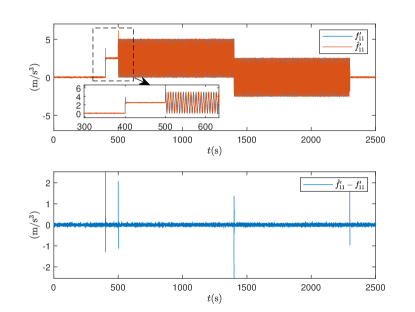
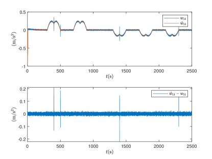
Figure 2: Top: profile of the fault and its estimation of the carriage $(1,1)$; bottom: profile of the estimation error.

Figure 3: Top: profile of the acceleration and its estimation of the carriage $(1,1)$; bottom: profile of the estimation error.

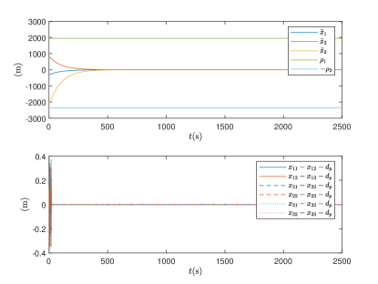
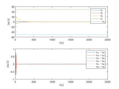
Figure 4: Top: profile of position difference of adjacent trains; bottom: profile of position difference of adjacent carriages.

Figure 5: Top: profile of velocity difference of adjacent trains; bottom: profile of velocity difference of adjacent carriages.

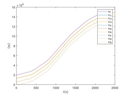
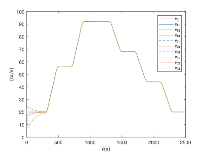
Figure 6: Profile of the desired position $x_{0}$ and the positions $x_{ij}$, $i=1,2,3$, $j=1,2,3$, of all the carriages.

Figure 7: Profile of the desired velocity $v_{0}$ and the velocities $v_{ij}$, $i=1,2,3$, $j=1,2,3$, of all the carriages.

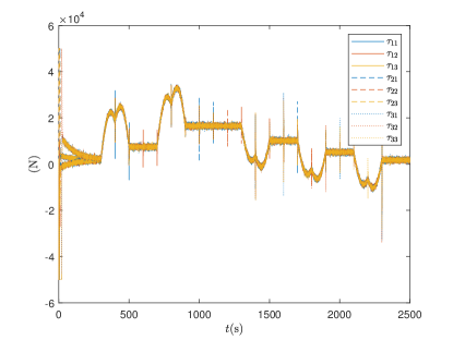
Figure 8: Profile of the traction/braking forces $\tau_{ij}$, $i=1,2,3$, $j=1,2,3$, of all the carriages.

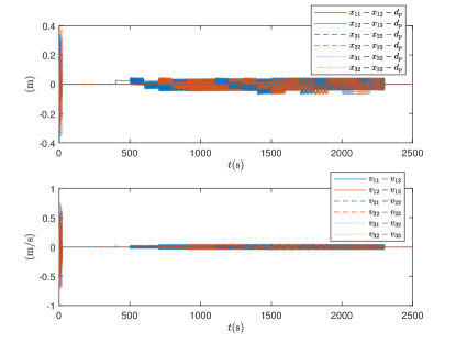
Figure 9: Profile of position and velocity differences of adjacent carriages using the observer in Zhu et al. (2015).

6 Conclusion

In this paper, a third-order HST multi-particle model with actuator faults has been established considering the motor dynamics of a real train. The structural information of the faults is also described by the model. Based on this model, an observer for asymptotical estimation of system states and a distributed fault-tolerant controller have been designed to realize cooperative cruise control under the dual constraints of ensuring the position and velocity differences of adjacent trains in specified ranges during the whole operation.

References

• Bai et al. (2021a) Bai, W., Dong, H., Lü, J., and Li, Y. (2021a). Event-triggering communication based distributed coordinated control of multiple high-speed trains. IEEE Transactions on Vehicular Technology, 70(9), 8556–8566.
• Bai et al. (2021b) Bai, W., Dong, H., Zhang, Z., and Li, Y. (2021b). Coordinated time-varying low gain feedback control of high-speed trains under a delayed communication network. IEEE Transactions on Intelligent Transportation Systems, 23(5), 4331–4341.
• Bai et al. (2020) Bai, W., Lin, Z., and Dong, H. (2020). Coordinated control in the presence of actuator saturation for multiple high-speed trains in the moving block signaling system mode. IEEE transactions on vehicular technology, 69(8), 8054–8064.
• Cao and Song (2020) Cao, Y. and Song, Y. (2020). Performance guaranteed consensus tracking control of nonlinear multiagent systems: A finite-time function-based approach. IEEE Transactions on Neural Networks and Learning Systems, 32(4), 1536–1546.
• Cao et al. (2021) Cao, Y., Wen, J., and Ma, L. (2021). Tracking and collision avoidance of virtual coupling train control system. Future Generation Computer Systems, 120, 76–90.
• Cascetta et al. (2020) Cascetta, E., Cartenì, A., Henke, I., and Pagliara, F. (2020). Economic growth, transport accessibility and regional equity impacts of high-speed railways in italy: Ten years ex post evaluation and future perspectives. Transportation Research Part A: Policy and Practice, 139, 412–428.
• Di Meo et al. (2019) Di Meo, C., Di Vaio, M., Flammini, F., Nardone, R., Santini, S., and Vittorini, V. (2019). Ertms/etcs virtual coupling: proof of concept and numerical analysis. IEEE transactions on intelligent transportation systems, 21(6), 2545–2556.
• Dong et al. (2016) Dong, H., Gao, S., and Ning, B. (2016). Cooperative control synthesis and stability analysis of multiple trains under moving signaling systems. IEEE Transactions on Intelligent Transportation Systems, 17(10), 2730–2738.
• Felez et al. (2019) Felez, J., Kim, Y., and Borrelli, F. (2019). A model predictive control approach for virtual coupling in railways. IEEE Transactions on Intelligent Transportation Systems, 20(7), 2728–2739.
• Gao et al. (2018) Gao, S., Dong, H., Ning, B., and Zhang, Q. (2018). Cooperative prescribed performance tracking control for multiple high-speed trains in moving block signaling system. IEEE Transactions on Intelligent Transportation Systems, 20(7), 2740–2749.
• Ge et al. (2019) Ge, M., Song, Q., Hu, X., and Zhang, H. (2019). Rbfnn-based fractional-order control of high-speed train with uncertain model and actuator failures. IEEE Transactions on Intelligent Transportation Systems, 21(9), 3883–3892.
• Goverde et al. (2016) Goverde, R.M., Bešinović, N., Binder, A., Cacchiani, V., Quaglietta, E., Roberti, R., and Toth, P. (2016). A three-level framework for performance-based railway timetabling. Transportation Research Part C: Emerging Technologies, 67, 62–83.
• Jikang et al. (2017) Jikang, X., Sen, J., and Yan, X. (2017). Switch control function of new cbts system developed based on train-train communication. Railway Signalling Commun. Eng., 3, 16.
• Li et al. (2015) Li, S., Yang, L., and Gao, Z. (2015). Coordinated cruise control for high-speed train movements based on a multi-agent model. Transportation Research Part C: Emerging Technologies, 56, 281–292.
• Li et al. (2020) Li, Y., Chen, Z., and Wang, P. (2020). Impact of high-speed rail on urban economic efficiency in china. Transport Policy, 97, 220–231.
• Li and Duan (2017) Li, Z. and Duan, Z. (2017). Cooperative control of multi-agent systems: a consensus region approach. CRC press.
• Lin et al. (2018) Lin, X., Dong, H., Yao, X., and Cai, B. (2018). Adaptive active fault-tolerant controller design for high-speed trains subject to unknown actuator faults. Vehicle system dynamics, 56(11), 1717–1733.
• Liu et al. (2019) Liu, S., Jiang, B., Mao, Z., and Ding, S.X. (2019). Adaptive backstepping based fault-tolerant control for high-speed trains with actuator faults. International Journal of Control, Automation and Systems, 17(6), 1408–1420.
• Mao et al. (2017) Mao, Z., Tao, G., Jiang, B., and Yan, X.G. (2017). Adaptive compensation of traction system actuator failures for high-speed trains. IEEE Transactions on intelligent transportation systems, 18(11), 2950–2963.
• Mao et al. (2019) Mao, Z., Yan, X.G., Jiang, B., and Chen, M. (2019). Adaptive fault-tolerant sliding-mode control for high-speed trains with actuator faults and uncertainties. IEEE Transactions on Intelligent Transportation Systems, 21(6), 2449–2460.
• Schumann (2017) Schumann, T. (2017). Increase of capacity on the shinkansen high-speed line using virtual coupling. International Journal of Transport Development and Integration, 1(4), 666–676.
• Song and Schnieder (2018) Song, H. and Schnieder, E. (2018). Development and evaluation procedure of the train-centric communication-based system. IEEE Transactions on Vehicular Technology, 68(3), 2035–2043.
• Song and Schnieder (2019) Song, H. and Schnieder, E. (2019). Availability and performance analysis of train-to-train data communication system. IEEE Transactions on Intelligent Transportation Systems, 20(7), 2786–2795.
• Song et al. (2013) Song, Y.D., Song, Q., and Cai, W.C. (2013). Fault-tolerant adaptive control of high-speed trains under traction/braking failures: A virtual parameter-based approach. IEEE Transactions on Intelligent Transportation Systems, 15(2), 737–748.
• Unterhuber et al. (2018) Unterhuber, P., Sand, S., Fiebig, U.C., and Siebler, B. (2018). Path loss models for train-to-train communications in typical high speed railway environments. IET Microwaves, Antennas & Propagation, 12(4), 492–500.
• Wang et al. (2019) Wang, X., Zhu, L., Wang, H., Tang, T., and Li, K. (2019). Robust distributed cruise control of multiple high-speed trains based on disturbance observer. IEEE Transactions on Intelligent Transportation Systems, 22(1), 267–279.
• Wang et al. (2013) Wang, Y., De Schutter, B., van den Boom, T.J., and Ning, B. (2013). Optimal trajectory planning for trains–a pseudospectral method and a mixed integer linear programming approach. Transportation Research Part C: Emerging Technologies, 29, 97–114.
• Yao et al. (2018) Yao, X., Wu, L., and Guo, L. (2018). Disturbance-observer-based fault tolerant control of high-speed trains: A markovian jump system model approach. IEEE Transactions on Systems, Man, and Cybernetics: Systems, 50(4), 1476–1485.
• Zhang and Chen (2022) Zhang, Z. and Chen, Z. (2022). Fault estimation and tolerant control of a class of nonlinear systems and its application in high-speed trains. IEEE Transactions on Control Systems Technology, under review.
• Zhao et al. (2017) Zhao, Y., Wang, T., and Karimi, H.R. (2017). Distributed cruise control of high-speed trains. Journal of the Franklin Institute, 354(14), 6044–6061.
• Zhu et al. (2015) Zhu, J.W., Yang, G.H., Wang, H., and Wang, F. (2015). Fault estimation for a class of nonlinear systems based on intermediate estimator. IEEE Transactions on Automatic Control, 61(9), 2518–2524.
• Zhu et al. (2022) Zhu, L., Li, X., Huang, D., Dong, H., and Cai, L. (2022). Distributed cooperative fault-tolerant control of high-speed trains with input saturation and actuator faults. IEEE Transactions on Intelligent Vehicles.