Automated Vehicle Highway Merging: Motion Planning via Adaptive Interactive Mixed-Integer MPC

Abstract

A new motion planning framework for automated highway merging is presented in this paper. To plan the merge and predict the motion of the neighboring vehicle, the ego automated vehicle solves a joint optimization of both vehicle costs over a receding horizon. The non-convex nature of feasible regions and lane discipline is handled by introducing integer decision variables resulting in a mixed integer quadratic programming (MIQP) formulation of the model predictive control (MPC) problem. Furthermore, the ego uses an inverse optimal control approach to impute the weights of neighboring vehicle cost by observing the neighbor’s recent motion and adapts its solution accordingly. We call this adaptive interactive mixed integer MPC (aiMPC). Simulation results show the effectiveness of the proposed framework.

I INTRODUCTION

One of the major challenges in autonomous driving is anticipation of neighboring vehicles’ (NV) behavior. The actions of the ego vehicle affect and are affected by the actions of neighboring vehicles [1]. This mutual influence of driving behavior is called interaction.

The motion planning problem in vehicle merging is particularly a problem where the coupling is significant as there is a strong mutual influence between the ego vehicle and its neighbor(s). Unilateral ‘pipeline’ based approaches do not consider the ability of the ego to influence the trajectory of the NV. Common unilateral approaches [2] include assumption of constant speed, constant acceleration, speed-dependent acceleration or intention sharing by NV through V2V connectivity [3]. The deviations from reality may be handled through probabilistic models [4, 5]. However, these approaches tend to be conservative since the motion plans are computed based on models of NV as if it acts in isolation. On the other hand, intention sharing through V2V communication involves practical challenges. The NV may not follow its shared intentions and it may be impractical in highway scenarios where intention sharing may not be possible due to the lack of network availability. Authors in some of the previous research work have recognized this limitation of traditional motion planning approaches. [6] presented a joint collision avoidance approach for robots. [7] presents an interactive merge management system with a relatively coarse decision space. It considers only the longitudinal control of the ego vehicle and does not incorporate system constraints explicitly.

Inspired by recent research [8, 9], in this paper we present an optimal control and inverse optimal control based method for interactive motion planning in automated driving highway merging. Our method not only incorporates the interactions, but also adapts the joint optimization cost function based on observation of the actual trajectory of the NV, online. Our hypothesis is that the nature of the NV is defined by weight it places on various terms in its cost function. These weights need to be estimated online through trajectory observations. To facilitate this, we harness the inverse optimization theory presented in [10].

Figure 1 visually represents our method when there is a single NV. The ego (blue) vehicle observes the immediate NV (red) for a few time instants and using the observed trajectory, imputes a cost function. It then utilizes this imputed cost function in a joint mixed integer MPC resulting in an interactive predictive control strategy. Our proposed framework requires only the current states of the NV which may be obtained either via V2V connectivity or on-board sensors. This makes the approach applicable to scenarios involving unconnected vehicles and out of network-coverage areas.

The paper is organized as follows: Section II presents the interactive joint MPC problem formulation. The simulation model of the NV is also presented. Next, in section III we briefly discuss the inverse optimization theory for online estimation of NV’s cost function and its implementation in the paper. Finally, in section IV we present simulation results that show the effectiveness of our proposed framework in online estimation of NV’s behavior, interactive motion planning and executing safe merging.

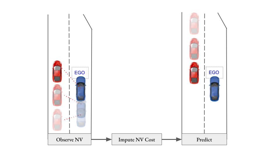
Figure 1: Schematic diagram of the proposed framework

II INTERACTION MODELING

In order to capture the interaction, we formulate the motion planning problem as a joint mixed-integer quadratic program (MIQP), solved in a receding horizon fashion via MPC. The cost terms associated with the NV are adapted online and therefore, we call this adaptive interactive mixed-integer MPC (aiMPC).

$$\begin{split}\min_{\tiny{u_{ego},u_{NV},\sigma_{logic}}}\sum_{i=k}^{k+N-1}J_{ego}(x_{ego}(i),u_{ego}(i))\\ +\;J_{NV}(\alpha,x_{NV}(i),u_{NV}(i))+J^{Terminal}\end{split}$$ (1a)

$$s.t.\;\;\;\;\;x_{ego}(i+1)=A_{d}x_{ego}(i)+B_{d}u_{ego}(i)$$ (1b)

$$\;\;\;\;\;x_{NV}(i+1)=A_{d,NV}x_{NV}(i)+B_{d,NV}u_{NV}(i)$$ (1c)

$$x_{vehicle}(i)\in\mathrm{X}_{free}$$ (1d)

$$u_{vehicle}(i)\in\mathrm{U}$$ (1e)

$$\sigma_{logic}(i)\in\{0,1\}$$ (1f)

where, $J_{vehicle},\;x_{vehicle},\;u_{vehicle}$ and $\sigma_{logic}$ are the quadratic cost, states, controls and logical variables respectively with $vehicle\in\{ego,NV\}$. $\alpha$ is the vector of weights estimated online, $X_{free}$ is the safe region to avoid collision and $U$ is the set of admissible controls.

The aiMPC formulation is based on [3]. However, unlike [3], in this paper we do not assume that the intention of the NV is shared with the ego. Instead, the joint cost, dynamics and collision avoidance constraints predict the trajectory of the ego and NV - capturing the mutual influence over the MPC horizon. The states of the NV are re-initialized according to the actual observation at every time step. This acts as feedback to the controller.

II-A The Cost Function

The cost function of the aiMPC includes the cost function of the ego as well as the NV. In this work, we limit our analysis to one NV, but the framework can be extended to multiple immediate NVs. The cost function used here assumes that the vehicles have already been assigned a driving schedule which translates to reference velocity and position. This is consistent with the literature [11] and involves minimizing the difference between the actual and reference state.

$$\begin{split}J_{ego}=q_{s,ego}(s_{ego}-s_{ref})^{2}+q_{v,ego}(v_{ego}-v_{ref})^{2}+\\ q_{a,ego}a_{ego}^{2}+q_{l,ego}(l_{ego}-l_{ref})^{2}+q_{a,ego}u_{a,ego}^{2}\end{split}$$ (2a)

$$J_{NV}=\alpha_{s}(s_{NV}-s_{ref,NV})^{2}+\alpha_{v}(v_{NV}-v_{ref,NV})^{2}+\alpha_{a}a_{NV}^{2}$$ (2b)

II-B Vehicle Model

Since this is a high level motion planner, consistent with the state of the art, we use a moderate fidelity kinematic model.

II-B1 Ego

The model we use for the ego vehicle was developed by Dollar et al [3] and decouples the lateral and longitudinal dynamics.

$$\small{\frac{d}{dt}\begin{bmatrix}s\\ v\\ a\\ l\\ r_{l}\end{bmatrix}=\begin{bmatrix}0&1&0&0&0\\ 0&0&1&0&0\\ 0&0&-\frac{1}{\tau}&0&0\\ 0&0&0&0&1\\ 0&0&0&-\omega_{n}^{2}&-2\zeta\omega_{n}\end{bmatrix}\begin{bmatrix}s\\ v\\ a\\ l\\ r_{l}\end{bmatrix}+\begin{bmatrix}0&0\\ 0&0\\ \frac{1}{\tau}&0\\ 0&0\\ 0&K\omega_{n}^{2}\end{bmatrix}\begin{bmatrix}u_{a}\\ u_{l}\end{bmatrix}}$$ (3)

The vehicle’s longitudinal motion is considered as a double integrator with the states being position, velocity and acceleration, $[s,v,a]$, and time constant $\tau$, while the lateral motion is cast as a second-order critically damped system with $[l,r_{l}]$ being the lateral lane position and rate of change of lane respectively. $\zeta$ is the damping ratio, $K$ is the gain and $\omega_{n}$ is the natural frequency. The control inputs are longitudinal acceleration $u_{a}$ and lane command $u_{l}$. It may be specified that $u_{l}$ is an integer equal to the commanded lane number. We discretize these dynamics when implementing in the controller as $x_{ego}(k+1)=A_{d}x_{ego}(k)+B_{d}u_{ego}(k)$ where $x_{ego}=[s\;v\;a\;l\;r_{l}]^{T}$ and $u_{ego}=[u_{a}\;u_{l}]^{T}$.

II-B2 NV

The dynamics of the NV (used in joint optimization by ego) are modeled as,

$$\frac{d}{dt}\begin{bmatrix}s_{NV}\\ v_{NV}\\ a_{NV}\end{bmatrix}=\begin{bmatrix}0&1&0\\ 0&0&1\\ 0&0&-\frac{1}{\tau}\end{bmatrix}\begin{bmatrix}s_{NV}\\ v_{NV}\\ a_{NV}\end{bmatrix}+\begin{bmatrix}0\\ 0\\ \frac{1}{\tau}\end{bmatrix}u_{NV}$$ (4)

These continuous time dynamics are discretized as $x_{NV}(k+1)=A_{d,NV}x_{NV}(k)+B_{d,NV}u_{NV}(k)$ where $x_{NV}=[s\;v\;a]^{T}$ and $u_{NV}$ is the longitudinal acceleration control. In this work we assume that the NV drives in its own lane.

TABLE I: Model parameters

Parameter	Value
$\tau$	0.275 s
$\omega_{n}$	1.091 rad/s
$\zeta$	1
$K$	1

II-C Joint Collision Avoidance Constraints

The drive-able region $X_{free}$ is non-convex. If in the same lane as NV, the ego vehicle either needs to be ahead of the front of NV or behind the rear of NV. We utilize the Big M method [12] to convert this OR constraint to AND, making it suitable for mixed integer programming.

$$s_{ego}-s_{NV}-M\beta_{l}^{NV}-M\mu_{l}\geq(L+gap)-2M$$ (5a)

$$s_{NV}-s_{ego}+M\beta_{l}^{NV}-M\mu_{l}\geq(L+gap)-M$$ (5b)

In equation (5), we introduce the logical decision variables $\beta_{l}^{NV}$ and $\mu_{l}$. $\beta_{l}^{NV}$ is the front-rear indicator. The choice of $1$ places ego ahead of the NV in lane $l$ and $0$ places it behind. $\mu_{l}$ is the lane indicator. If set to $1$, ego resides in the lane $l$ and if set to $0$ it does not. In effect, the equation (5a) ensures that ego maintains a distance equal to the vehicle length $L$ plus a desired $gap$ ahead of the NV when it is placed in the same lane and ahead of NV. When this is the case, (5b) gets inactive. On the other hand, when ego resides behind NV, (5b) ensures that it maintains $L+gap$ behind it while (5a) gets inactive.

II-D Control Admissibility

The acceleration control admissibility constraints combine velocity with the acceleration command to prevent operation in mechanically infeasible regions [13].

$$u_{a}\geq u_{a,min}$$ (6a)

$$u_{a}\leq m_{1}v+b_{1}$$ (6b)

$$u_{a}\leq m_{2}v+b_{2}$$ (6c)

Here, the maximal acceleration is velocity dependent and (6) is a convex approximation to the feasible region.

II-E Simulating the Neighbor

For this work, we simulate the NV as controlled by an MPC which solves the following quadratically constrained quadratic program (QCQP)

$$\min_{u_{NV}^{actual}}\sum_{i=k}^{k+T-1}J_{NV}(q,x_{NV}(i),x_{ego}(i),u_{NV}^{actual}(i))$$ (7a)

$$s.t.\;\;\;\;\;x_{NV}(k+1)=A_{d,NV}x_{NV}(k)+B_{d,NV}u_{NV}^{actual}(k)$$ (7b)

$$\;\;\;\;\;x_{ego}(i+1)=g_{projection}(x_{ego}(i))$$ (7c)

$$x_{NV}(i)\in\mathcal{X}_{free}$$ (7d)

$$u_{NV}^{actual}(i)\in\mathcal{U}$$ (7e)

$$\mathcal{X}_{free}\doteq\dfrac{(s_{NV}(i)-s_{ego}(i))^{2}}{a^{2}}+\dfrac{(l_{NV}(i)-l_{ego}(i))^{2}}{b^{2}}\geq 1$$ (7f)

Physically, this translates to the NV projecting the ego vehicle into the future to predict its trajectory over the horizon via the $g_{projection}()$ function. This function determines the future longitudinal and lateral position of the ego from the current observed states. In this work, we assume that the NV projects the ego by holding the current longitudinal ($v$) and lateral ($r_{l}$) velocity constant over the horizon. The NV controller also maintains a safety distance from the ego by ensuring that it lies outside an ellipse encapsulating the ego with semi-major axis $a$, semi-minor axis $b$ and centered on the ego. Other expressions have the same meaning as before while it may be noted that $u_{NV}^{actual}$ is the actual control applied by NV which is not available to the ego.

III ESTIMATING NEIGHBOR BEHAVIOR

Inspired by previous research [8], we aim to estimate the behavior of the neighboring vehicle (NV) online by observing its trajectory. In the present problem, we define behavior based on weights associated with various terms in the cost function of the NV. Our approach imputes [10] these cost parameters (weights) based on the observed trajectory (data).

III-A Background

In order to keep the paper reasonably self contained, we give a brief background on imputing a convex objective function from data. The detailed theory can be found in [10].

The aim is to fit a convex forward optimization problem (8) to the observed trajectory data,

$$\min_{x}f(x)$$ (8a)

$$s.t.\;h(x,u)=0$$ (8b)

$$g_{j}(x,u)\leq 0\;forj=1,...,p$$ (8c)

where $x\in\mathbb{R}^{n}$ are the state data, $u\in\mathbb{R}^{m}$ are the controls, $f(x)$ is a convex function, $h(x,u)$ is linear in $x$ and $u$ and $g_{j}$ are convex. Assuming that the observed trajectory is approximately optimal with respect to problem (8), we define residuals based on the Karush–Kuhn–Tucker (KKT) conditions. These residuals are deviations from the first order necessary conditions of optimality.

$$r_{eq}=h(x,u)$$ (9a)

$$r_{ineq}=(g_{j}(x,u))_{+}$$ (9b)

$$r_{stat}(\alpha,\lambda,\nu)=\nabla f(x)+\Sigma_{j=1}^{p}\lambda_{j}\nabla g_{j}(x,u)+\nu h(x,u)$$ (9c)

$$r_{comp}(\lambda)=\lambda_{j}g_{j}(x,u),\;\;\;j=1,...,p$$ (9d)

Here, $r_{eq}$ and $r_{ineq}$ are the primal feasibility conditions which are independent of the dual variables. We assume they are close to zero. Now, for the observed trajectory to be approximately optimal, the residuals $r_{stat}$ and $r_{comp}$ are minimized. The dual variables $\lambda,\nu$ and the imputation parameter $\alpha$ are the decision variables and

$$f=\sum_{j}\alpha_{j}f_{j},\;\;\;\alpha=[\alpha_{1},...,\alpha_{j}]$$ (10a)

where $f_{j}$ are the basis functions of the cost function. Our goal is to find $\alpha$ for which $f$ is (approximately) consistent with the observed trajectory data.

III-B Formulation

We fit the following optimization problem to the observed trajectory.

$$\min_{x_{NV}^{(i+1)}}\sum_{i=k-r}^{k-1}J_{NV}(\alpha,x_{NV}^{(i+1)})$$ (11a)

$$s.t.\;\;\;h(x_{NV}^{(i+1)},x_{NV}^{(i)},u_{NV}^{(i)})=0$$ (11b)

$$g_{j}(x_{NV}^{(i+1)},x_{Ego}^{(i+1)},u_{NV}^{(i)})\leq 0,\;\;\;j=1,...,p$$ (11c)

where, $k$ is the current time step and the ego vehicle has observed the trajectory of the NV for previous $r$ time steps. $h$ captures the NV vehicle dynamics and $g_{j}$ are the convex inequality constraints in the NV’s optimization problem. Other expressions have the same meaning as before and we denote trajectory data time step in the superscript.

With this, the residuals to be minimized are

$$r_{stat}(\alpha,\lambda,\nu)=\Sigma_{i=k-r}^{k}[\nabla J_{NV}+\Sigma_{j}\lambda_{j}\nabla g_{j}+\Sigma_{j}\nu_{j}\nabla h_{j}]$$ (12a)

$$r_{comp}(\lambda)=\Sigma_{i=k-r}^{k}\lambda_{j}g_{j},\;\;\;j=1,...,p$$ (12b)

Note that in our formulation, we fit a problem (11) such that only the state trajectory data of NV is required. Specifically, problem (11) is carefully chosen such that equation (12) results in the residuals containing only the state trajectory terms. This is vital for practical implementation since the control data of NV may not be easily available.

Finally, the following convex optimization problem is solved to impute the cost function based on the trajectory data.

$$\min_{\alpha}\|r_{stat}\|_{2}^{2}+\|r_{comp}\|_{2}^{2}$$ (13a)

$$s.t.\;\;\;\alpha_{s},\alpha_{v},\alpha_{a}\geq 0$$ (13b)

$$\lambda_{j}\geq 0$$ (13c)

$$\alpha_{s}+\alpha_{v}+\alpha_{a}=1$$ (13d)

IV SIMULATION RESULTS

We test our method in simulation. A 2-lane highway with on-ramp is considered where the ego vehicle (blue) needs to negotiate a merge with the NV (red). The aiMPC is invoked at a configuration where which vehicle should yield is ambiguous. As discussed in literature, in the cases where the two cars are close in longitudinal direction and have similar speed, successfully executing the merging maneuver is a very challenging task [14]. This challenge stems from the unknown future trajectory of the NV and its unknown nature. We test various cases with NV’s nature defined by the position, velocity and acceleration weights: $q_{s},q_{v}$ and $q_{a}$, respectively, in its cost function. Qualitatively, for instance, when $q_{v}=1$ the NV is aggressive while when $q_{a}=1$ the NV is conservative in its driving.

The MPC and imputation problems are solved using GUROBI^™ on a PC with Intel^® Core^™ i7-10750H CPU @ 2.60GHz and 8 GB RAM.

TABLE II: Simulation parameters

Simulation Parameter	Value
Simulation time	$8\;s$
Sampling time	$400\;ms$
$N$ (Ego Horizon)	$15\;(6s)$
$T$ (NV Horizon)	$3\;(1.2s)$
$r$ (Trajectory Observation)	$3\;(1.2s)$

Figure 2: The simulation process flow of information

IV-A Comparison with constant velocity and constant acceleration models

We compare our method to constant velocity and constant acceleration models of NV. These are the baseline cases where the ego vehicle assumes that the NV remains at the current observed velocity and acceleration respectively, over the MPC horizon, at each time instant. The results of an edge case scenario (Table III) are shown.

TABLE III: Simulation A conditions

NV Nature	$(q_{s},q_{v},q_{a})$	$v_{0,ego}[m/s]$	$v_{0,NV}[m/s]$	Method	Result
Aggressive	(0, 1, 0)	10	12	Constant velocity non-interactive	Ego unable to merge
Aggressive	(0, 1, 0)	10	12	Constant acceleration non-interactive	Ego unable to merge
Aggressive	(0, 1, 0)	10	12	aiMPC	Ego merges behind $46.6\%$ less hindraance

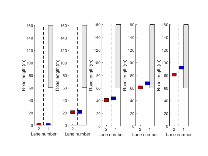
Figure 3: Constant velocity model for NV (Red): Ego (Blue) unable to merge

Figure 4: Constant acceleration model for NV (Red): Ego (Blue) unable to merge

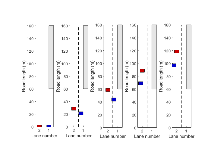
Figure 5: aiMPC: Ego (Blue) merges behind NV (Red) and reduces hindrance to NV

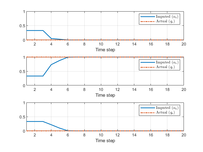
Figure 6: aiMPC imputation results: initialized with equi-weighted cost and adapted online based on trajectory observations

We observe that the ego vehicle is unable to merge in the baseline cases and also causes hindrance for the NV (Fig. 3, Fig. 4). On the other hand, motion planning via aiMPC results in successful merging and reduced hindrance (Fig. 5). The hindrance to NV is reduced by $46.6\%$ (travel distance increased), which reflects socially compliant driving. This highlights the utility of interactive motion planning. Fig. 6 shows the online imputation results of NV’s cost by the ego which are utilized in the interactive planning.

IV-B Comparison with Non-adaptive MPC

Next, we test the significance of estimating the nature of NV via the imputation method presented in the paper. We perform two simulations: one with equi-weighted cost of NV which remains constant throughout, and the other with (adaptive) online imputation of the cost.

TABLE IV: Simulation B conditions

NV Nature	$(q_{s},q_{v},q_{a})$	$v_{0,ego}[m/s]$	$v_{0,NV}[m/s]$	Method	Result
Conservative	(0, 0, 1)	11	10	Non-adaptive	Ego merges ahead but jerky
Conservative	(0, 0, 1)	11	10	aiMPC	Ego merges ahead smoother

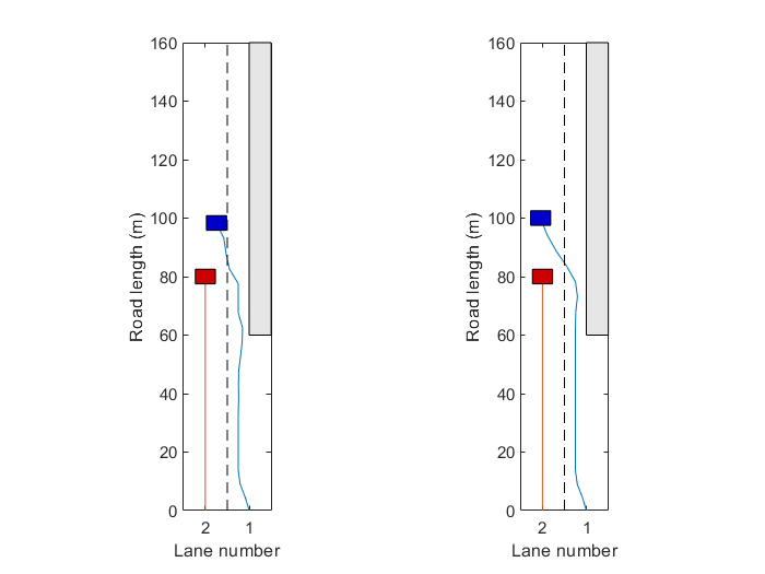
Figure 7: Non-adaptive cost (left) results in tentative motion while aiMPC (right) results in smoother motion

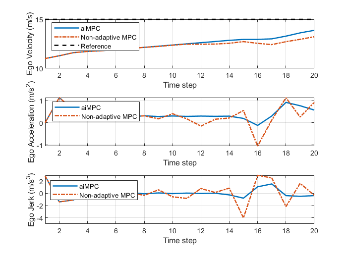
Figure 8: Ego is able to reach nearer to reference velocity and with lower jerk when the cost is adapted via online imputation

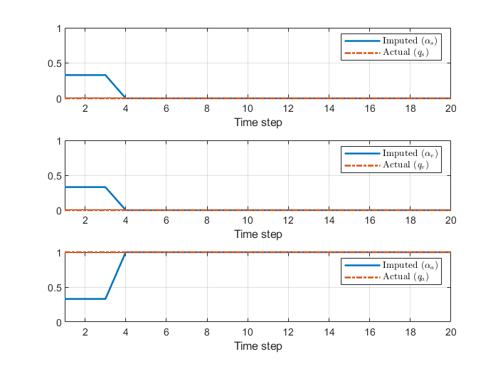
Figure 9: aiMPC imputation results: initialized with equi-weighted cost and adapted online based on trajectory observations

In the first case (Fig. 7), the ego merges ahead but the trajectory is not smooth. This tentative motion is due to the larger prediction error in the joint MPC because of the cost function mismatch. In the second case (Fig. 7) the cost is imputed and adapted online. This leads to more accurate predictions in the joint MPC, resulting in more confident and smooth motion quantified through lower jerk (Fig. 8). Fig. 9 shows the online imputation results for this case.

IV-C Moderate nature of NV

We also test a mixed case where NV has a moderate nature and places equal weightage on aggressiveness and conservativeness i.e. $q_{v}=0.5$ and $q_{a}=0.5$.

TABLE V: Simulation C conditions

NV Nature	$(q_{s},q_{v},q_{a})$	$v_{0,ego}[m/s]$	$v_{0,NV}[m/s]$	Method	Result
Moderate	(0, 0.5, 0.5)	10	10	Non-adaptive	Ego unable to merge
Moderate	(0, 0.5, 0.5)	10	10	aiMPC	Ego merges behind

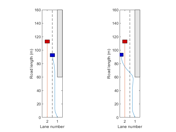
Figure 10: Nonadaptive MPC unable to merge in time (left) while aiMPC facilitates successful merging (right)

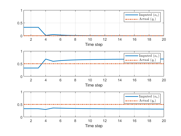
Figure 11: aiMPC does not converge to exact NV nature but the approximate imputation facilitates timely merging

In this case, the imputation cost does not converge exactly to the actual nature of NV (Fig. 11), but the close approximation facilitates successful merging as shown in Fig. 10.

V CONCLUSIONS

We presented a new optimal control and inverse optimal control based framework for motion planning of automated vehicles interacting with neighboring vehicles. We focused on highway merging scenario due to the significant interactive challenges it presents. The proposed framework was tested in simulation and the results highlight the utility and significance of motion planning via interactive, online estimation based adaptive cost identifying MPC in highway merging. Future work involves identification of higher fidelity cost functions and testing of the proposed framework in vehicle-in-the-loop tests.

References

- [1] J. F. Fisac, E. Bronstein, E. Stefansson, D. Sadigh, S. S. Sastry, and A. D. Dragan, “Hierarchical game-theoretic planning for autonomous vehicles,” in 2019 International conference on robotics and automation (ICRA), pp. 9590–9596, IEEE, 2019.
- [2] A. Sciarretta and A. Vahidi, “Perception and control for connected and automated vehicles,” in Energy-Efficient Driving of Road Vehicles, pp. 63–82, Springer, 2020.
- [3] R. A. Dollar and A. Vahidi, “Predictively coordinated vehicle acceleration and lane selection using mixed integer programming,” in Dynamic Systems and Control Conference, vol. 51890, p. V001T09A006, American Society of Mechanical Engineers, 2018.
- [4] F. Havlak and M. Campbell, “Discrete and continuous, probabilistic anticipation for autonomous robots in urban environments,” IEEE Transactions on Robotics, vol. 30, no. 2, pp. 461–474, 2013.
- [5] R. A. Dollar and A. Vahidi, “Automated vehicles in hazardous merging traffic: A chance-constrained approach,” IFAC-PapersOnLine, vol. 52, no. 5, pp. 218–223, 2019.
- [6] P. Trautman and A. Krause, “Unfreezing the robot: Navigation in dense, interacting crowds,” in 2010 IEEE/RSJ International Conference on Intelligent Robots and Systems, pp. 797–803, IEEE, 2010.
- [7] B. B. Litkouhi, J. Wei, and J. M. Dolan, “Autonomous driving merge management system,” U.S. Patent 8 788 134, Jul. 2014.
- [8] W. Schwarting, A. Pierson, J. Alonso-Mora, S. Karaman, and D. Rus, “Social behavior for autonomous vehicles,” Proceedings of the National Academy of Sciences, vol. 116, no. 50, pp. 24972–24978, 2019.
- [9] D. Sadigh, N. Landolfi, S. S. Sastry, S. A. Seshia, and A. D. Dragan, “Planning for cars that coordinate with people: leveraging effects on human actions for planning and active information gathering over human internal state,” Autonomous Robots, vol. 42, no. 7, pp. 1405–1426, 2018.
- [10] A. Keshavarz, Y. Wang, and S. Boyd, “Imputing a convex objective function,” in 2011 IEEE international symposium on intelligent control, pp. 613–619, IEEE, 2011.
- [11] J. Rios-Torres and A. A. Malikopoulos, “A survey on the coordination of connected and automated vehicles at intersections and merging at highway on-ramps,” IEEE Transactions on Intelligent Transportation Systems, vol. 18, no. 5, pp. 1066–1077, 2016.
- [12] A. Vecchietti, S. Lee, and I. E. Grossmann, “Modeling of discrete/continuous optimization problems: characterization and formulation of disjunctions and their relaxations,” Computers & chemical engineering, vol. 27, no. 3, pp. 433–448, 2003.
- [13] R. A. Dollar and A. Vahidi, “Quantifying the impact of limited information and control robustness on connected automated platoons,” in 2017 IEEE 20th International Conference on Intelligent Transportation Systems (ITSC), pp. 1–7, IEEE, 2017.
- [14] M. Wang, N. Mehr, A. Gaidon, and M. Schwager, “Game-theoretic planning for risk-aware interactive agents,” in 2020 IEEE/RSJ International Conference on Intelligent Robots and Systems (IROS), pp. 6998–7005, IEEE, 2020.