Monotone Lagrangian Floer theory in smooth divisor complements: III

Abstract.

This is the third paper in a series of papers studying intersection Floer theory of Lagrangians in the complement of a smooth divisor. We complete the construction of Floer homology for such Lagrangians.

1. Introduction

Let $(X,\omega)$ be a compact symplectic manifold and $\mathcal{D}\subset X$ be a smooth divisor. That is to say, $\mathcal{D}$ is a codimension $2$ closed submanifold of $X$ such that the restriction of $\omega$ to $\mathcal{D}$ is non-degenerate. Before stating our main theorem, which is a slightly stronger version of [part1:top, Theorem 1], we recall the definition of some basic ingredients of the theorem.

Definition .

Let $L_{0},L_{1}$ be compact subspaces of $X\setminus\mathcal{D}$. We say $L_{0}$ is Hamiltonian isotopic to $L_{1}$ in $X\setminus\mathcal{D}$ if there exists a compactly supported time dependent Hamiltonian $H:(X\setminus\mathcal{D})\times[0,1]\to{\mathbb{R}}$ such that the Hamiltonian diffeomorphism $\psi_{H}:X\setminus\mathcal{D}\to X\setminus\mathcal{D}$ maps $L_{0}$ to $L_{1}$. Here $\psi_{H}$ is defined as follows. Let $H_{t}(x)=H(x,t)$ and $X_{H_{t}}$ be the Hamiltonian vector field associated to $H_{t}$. We define $\psi^{H}_{t}$ by

$$\psi^{H}_{0}(x)=x,\qquad\frac{d}{dt}\psi^{H}_{t}=X_{H_{t}}\circ\psi^{H}_{t}.$$

Then $\psi_{H}:=\psi^{H}_{1}$. We say that $\psi_{H}$ is the Hamiltonian diffeomorphism associated to the (non-autonomous) Hamiltonian $H$.

Definition .

Let $\Lambda^{{\mathbb{Q}}}$ denote the Novikov field of all formal sums

$$\sum_{i=1}^{\infty}a_{i}T^{\lambda_{i}},$$

where $a_{i}\in{\mathbb{Q}}$, $\lambda_{i}\in{\mathbb{R}}$, $\lambda_{i}<\lambda_{i+1}$ and $\lim_{i\to\infty}\lambda_{i}=+\infty.$

Now we state:

Theorem 1.

Let $L_{0},L_{1}\subset X\setminus\mathcal{D}$ be compact, oriented and spin Lagrangian submanifolds such that they are monotone in $X\setminus\mathcal{D}$. Suppose one of the following conditions holds:

1. The minimal Maslov numbers of $L_{0}$ and of $L_{1}$ are both strictly greater than 2.

2. $L_{1}$ is Hamiltonian isotopic to $L_{0}$.

Then we can define Floer homology group $HF(L_{1},L_{0};X\setminus\mathcal{D})$, which is a $\Lambda^{{\mathbb{Q}}}$-vector space, and satisfies the following properties.

1. If $L_{0}$ is transversal to $L_{1}$ then we have

   $${\rm rank}_{\Lambda^{{\mathbb{Q}}}}HF(L_{1},L_{0};X\setminus D)\leq\#(L_{0}\cap L_{1}).$$

2. If $L_{i}^{\prime}$ is Hamiltonian isotopic to $L_{i}$ in $X\setminus\mathcal{D}$ for $i=0,1$, then

   $$HF(L_{1},L_{0};X\setminus\mathcal{D})\cong HF(L^{\prime}_{1},L^{\prime}_{0};X\setminus\mathcal{D}).$$

3. If we assume either (b) or $\pi_{1}(L_{0})=\pi_{1}(L_{1})=0$, then we can replace $\Lambda^{{\mathbb{Q}}}$ with ${\mathbb{Q}}$, the field of rational numbers.

4. If $L_{0}=L_{1}=L$, then there exists a spectral sequence whose $E^{2}$ page is the singular homology group $H_{*}(L;{\mathbb{Q}})$ of $L$ and which converges to $HF(L,L;X\setminus\mathcal{D})$.

See Condition 2.1 (2) for the definition of the monotonicity of Lagrangians in $X\setminus\mathcal{D}$.

Remark .

The above theorem can be strengthened in various directions. In Theorem 1, we assumed $L_{i}$ is spin. We can relax this condition to the condition that $L_{i}\subset X\setminus\mathcal{D}$ is relatively spin and $(L_{1},L_{0})$ forms a relatively spin pair in $X\setminus\mathcal{D}$. (See [fooobook, Definition 3.1.1] for the definition of relatively spin Lagrangians and relatively spin pairs.)

Let $L$ be a monotone Lagrangian in $X\setminus\mathcal{D}$. Associated to any such Lagrangian, there is an element $\mathfrak{PO}_{L}(1)\in\Lambda^{{\mathbb{Q}}}$, which vanishes if minimal Maslov number of $L$ is not equal to $2$. The assumption in Item (a) can be also weakened to the assumption that $\mathfrak{PO}_{L_{0}}(1)=\mathfrak{PO}_{L_{1}}(1)$. We can also replace the assumption in Item (3), with the weaker assumption stated in Condition 2.1 (2).

Using the construction of Kuranishi structures in [part2:kura] on the moduli spaces we introduced in [part1:top], the proof of Theorem 1 is in principle a modification of the arguments of the construction of Lagrangian Floer theory based on virtual fundamental chain techniques. (See, for example, [fooobook2, fooonewbook].) It is also a variant of Oh’s construction of Floer homology of monotone Lagrangian submanifolds [oh].

There are, however, a few subtle technical points that need to be sorted out for the construction of our version of Floer homology. We highlight two of these points, which are more important than the other ones. The first one is related to the description of the boundary of the moduli spaces that are used in the definition of Lagrangian Floer homology. We will discuss this point in Sections 2 and 3. In our situation, the boundaries of the moduli spaces involved are not given as fiber products of the moduli spaces with smaller energy, but they only accept such descriptions outside codimension two strata. This is a new feature which does not seem to appear previously in the literature.

The second point is related to compatibility of our Kuranishi structures with certain forgetful maps. This point, which we will study in Section 4, needs to be addressed only when there are Maslov index 2 pseudo-holomorphic disks. Oh studied a similar problem in [oh], where he could use perturbation of almost complex structures to achieve transversality for the moduli spaces of pseudo-holomorphic curves. Therefore, compatibility with forgetful maps is immediate in his setup. Even though we are studying monotone Lagrangian submanifolds, we have to use virtual fundamental chain techniques and abstract perturbations. For this reason, compatibility with forgetful maps becomes a much more nontrivial problem.

The proof of Theorem 1 is completed in Section 5. In Subsection 5.1 the independence of Floer homology from auxiliary choices is proved. In Sections 2, 3, 4 we assume that not only $L_{0}$ and $L_{1}$ but also the pair $(L_{0},L_{1})$ satisfies a certain monotonicity condition (Condition 2.1 (2)). In Subsection 5.2 we remove this condition by using Novikov ring. Finally a spectal sequence calculating the Floer homology in case $L_{1}=L_{0}$ is defied in Subsection 5.3. Since the arguments of Section 5 are modifications of standard proofs, we sketch the proofs without going into details.

The final section of the paper is devoted to various possible extensions of our main result. In particular, we explain how we expect that one can associate an $A_{\infty}$-category to a family of Lagrangians in the complement of a smooth divisor, generalize the construction of this paper to the case of normal crossing divisors and define an equivariant version of Lagrangian Floer homology of Theorem 1. Perhaps the most interesting direction among the proposals in Section 6 is the extension of the present theory to the case of non-compact Lagrangians. In this part, we present some formal similarities between the proposed theory for non-compact Lagrangians and monopole Floer homology in [km:monopole].

Remark .

We remark that the proofs of various claims of this paper require a study of orientations of moduli spaces and the resulting signs in the formulas in several places. However, there is nothing novel about signs happening in our case. The key point here is that we only need to orient the part of the moduli space that is obtained from the zero set of perturbed multi-sections. Even though we use the existence of Kuranishi structures on the strata with arbitrary high codimension in our construction, we may arrange that the zero set of perturbed multi-sections consists of pseudo-holomorphic maps that do not intersect divisor. This allows us to adapt standard arguments to our setup without any new issue. Because of this, we skip the discussion of orientations and signs, and refer the reader to [fooobook2, Section 8] for more details.

2. Floer homology when minimal Maslov number is greater than 2.

2.1. The Definition of Floer Homology

Let $L_{0},L_{1}$ be Lagrangian submanifolds in $X\setminus\mathcal{D}$. We assume they are monotone in $X\setminus\mathcal{D}$ and are relatively spin there. We assume that $L_{0}$ is transversal to $L_{1}$. In Sections 2 and 3, we firstly work under the assumption of Condition 2.1 below, where we can use ${\mathbb{Q}}$ as the coefficient ring rather than the Novikov ring. We need to prepare some notations to state this condition.

Definition .

Let $\Omega(L_{0},L_{1})$ denote the space of all continuous maps $\gamma:[0,1]\to X$ with $\gamma(0)\in L_{0}$, $\gamma(1)\in L_{1}$. For $o\in\pi_{0}(\Omega(L_{0},L_{1}))$, we denote the fundamental group of the corresponding connected component by $\pi_{1}(\Omega(L_{0},L_{1});o)$. We also write $L_{0}\cap_{o}L_{1}$ for the subset of $L_{0}\cap L_{1}$ consisting of $p$ such that the constant map $\gamma(t)\equiv p$ belongs to the connected component $o$.

Definition .

An element of $\pi_{1}(\Omega(L_{0},L_{1});o)$ determines a relative second homology class $H_{2}(X,L_{0}\cup L_{1};{\mathbb{Z}})$. Since $(L_{0}\cup L_{1})\cap\mathcal{D}=\emptyset$, we obtain a map:

$$\cap\mathcal{D}:\pi_{1}(\Omega(L_{0},L_{1});o)\to{\mathbb{Z}}.$$

We may also integrate $\omega$ on homology classes represented by elements of $\pi_{1}(\Omega(L_{0},L_{1});o)$ to obtain another homomorphism

$$\omega:\pi_{1}(\Omega(L_{0},L_{1});o)\to{\mathbb{R}}.$$

Finally, we have the Maslov index homomorphism

$$\mu:\pi_{1}(\Omega(L_{0},L_{1});o)\to{\mathbb{Z}}.$$

(See, for example, [fooobook, p50], where it is denoted by $I_{\mu}$.)

Condition .

Let $o\in\pi_{0}(\Omega(L_{0},L_{1}))$ be given. We require the following two properties:

1. The minimum Maslov numbers of $L_{0}$ and $L_{1}$ are not smaller than 4.

2. There is a constant $c$ such that for any $\alpha\in\pi_{1}(\Omega(L_{0},L_{1}),o)$ with $\alpha\cap\mathcal{D}=0$, we have

   (2.1) $$\omega(\alpha)=c\mu(\alpha).$$

Lemma .

We assume Condition 2.1 (2) for $o\in\pi_{0}(\Omega(L_{0},L_{1}))$ holds. Then for each $p,q\in L_{0}\cap_{o}L_{1}$, there exists $c(p,q)$ such that:

(2.2) $$\omega(\beta)=c\mu(\beta)-c(p,q),$$

for any $\beta\in\Pi_{2}(X;L_{0},L_{1};p,q)$ with $\beta\cap\mathcal{D}=0$.

Proof.

Let $\beta_{1},\beta_{2}\in\Pi_{2}(X;L_{0},L_{1};p,q)$. Since $\beta_{2}$ is represented by a map ${\mathbb{R}}\times[0,1]\to X$, we can compose it with $(\tau,t)\mapsto(-\tau,t)$ and obtain $-\beta_{2}\in\Pi_{2}(X;L_{0},L_{1};q,p)$. We concatenate $\beta_{1}$ and $-\beta_{2}$ in an obvious way to obtain $\beta_{1}\#-\beta_{2}\in\pi_{1}(\Omega(L_{0},L_{1});o)$. It follows easily from definition that

$$\mu(\beta_{1})-\mu(\beta_{2})=\mu(\beta_{1}\#-\beta_{2}),\quad\omega(\beta_{1})-\omega(\beta_{2})=\omega(\beta_{1}\#-\beta_{2}).$$

The lemma follows easily from these identities. ∎

Lemma .

For $i=0$ or $1$, let $\pi_{1}(L_{i})$ be trivial. Then Condition 2.1 (2) holds for any $o$.

Proof.

Let $\alpha\in\pi_{1}(\Omega(L_{0},L_{1});o)$. It is represented by a map $u:S^{1}\times[0,1]\to X$ with $u(S^{1}\times\{i\})\subset L_{i}$ for $i=0,1$. We assume $\pi_{1}(L_{0})=0$. Then there exists a map $v:D^{2}\to L_{0}$ such that $v|_{S^{1}}=u_{S^{1}\times\{0\}}$. We glue $v$ and $u$ to obtain $v^{\prime}$. We have:

$$\mu([v])+\mu(\alpha)=\mu([v^{\prime}])\quad\omega([v])+\omega(\alpha)=\omega([v^{\prime}]).$$

Since $\mu([v])=\omega([v])=0$, Condition 2.1 (2) follows from the monotonicity of $L_{i}$. ∎

To prove Theorem 1, we use moduli spaces $\mathcal{M}^{\rm RGW}_{k_{1},k_{0}}(L_{1},L_{0};p,q;\beta)$ and $\mathcal{M}^{\rm RGW}_{k}(L;\alpha)$ introduced in [part1:top] and the construction of Kuranishi structures on these spaces obtained in [part2:kura]. These moduli spaces are defined as the union of spaces which are parametrized by combinatorial objects called SD-ribbon trees and DD-ribbon trees. We may evaluate a pseudo-holomorphic curve representing an element of the moduli space $\mathcal{M}^{\rm RGW}_{k_{1},k_{0}}(L_{1},L_{0};p,q;\beta)$ at the boundary marked points to obtain the evaluation maps

$${\rm ev}^{\partial}_{i,j}:\mathcal{M}^{\rm RGW}_{k_{1},k_{0}}(L_{1},L_{0};p,q;\beta)\to L_{i},$$

where $i\in\{0,1\}$ and $j\in\{1,2,\dots,k_{i}\}$. Similarly, we have evaluation maps

$${\rm ev}^{\partial}_{j}:\mathcal{M}^{\rm RGW}_{k}(L;\alpha)\to L,$$

for $j\in\{0,1,2,\dots,k\}$. We assume familiarity with the definitions of these notions and refer the reader to [part1:top, part2:kura] for more details. We also need the following result.

Theorem .

For any $\beta\in\Pi_{2}(X;L_{1},L_{0};p,q)$, then there is a Kuranishi structure on $\mathcal{M}^{\rm RGW}_{k_{1},k_{2}}(L_{1},L_{0};p,q;\beta)$ such that the normalized boundary of this space is the union of the following three types of ‘fiber or direct products’ (as spaces with Kuranishi structure).

1. $$\mathcal{M}^{\rm RGW}_{k^{\prime}_{1},k^{\prime}_{2}}(L_{1},L_{0};p,r;\beta_{1})\,\hat{\times}\,\mathcal{M}^{\rm RGW}_{k^{\prime\prime}_{1},k^{\prime\prime}_{2}}(L_{1},L_{0};r,q;\beta_{2}).$$

   Here $r\in L_{0}\cap L_{1}$, $k^{\prime}_{1}+k^{\prime\prime}_{1}=k_{1}$, $k^{\prime}_{2}+k^{\prime\prime}_{2}=k_{2}$, $\beta_{1}\in\Pi_{2}(X,L_{1},L_{0};p,r)$ and $\beta_{2}\in\Pi_{2}(X,L_{1},L_{0};r,q)$ such that $\beta_{1}\#\beta_{2}=\beta$ and $\beta_{1}\cdot[\mathcal{D}]=\beta_{2}\cdot[\mathcal{D}]=0$.( The symbol $\hat{\times}$ will be discussed in Subsection 2.2.)

2. $$\mathcal{M}^{\rm RGW}_{k^{\prime}_{1},k_{2}}(L_{1},L_{0};p,q;\beta^{\prime})\,\hat{\times}_{L_{1}}\,\mathcal{M}^{\rm RGW}_{k^{\prime\prime}_{1}+1}(L_{1};\alpha).$$

   Here $k^{\prime}_{1}+k^{\prime\prime}_{1}=k_{1}+1$, $\beta^{\prime}\in\Pi_{2}(X,L_{1},L_{0};p,q)$, $\alpha\in\Pi_{2}(X,L_{1};{\mathbb{Z}})$ form a pair such that $\beta^{\prime}\#\alpha=\beta$ and $\beta^{\prime}\cdot[\mathcal{D}]=\alpha\cdot[\mathcal{D}]=0.$ The ‘fiber product’ $\hat{\times}_{L_{1}}$ is defined using ${\rm ev}^{\partial}_{1,i}$, for $i=1,\dots,k^{\prime}_{1}$, and ${\rm ev}^{\partial}_{0}$. (Here $\hat{\times}_{L_{1}}$ is slightly different from the ordinary fiber product. See Subsection 2.2.)

3. $$\mathcal{M}^{\rm RGW}_{k_{1},k^{\prime}_{2}}(L_{1},L_{0};p,q;\beta^{\prime})\,\hat{\times}_{L_{0}}\,\mathcal{M}^{\rm RGW}_{k^{\prime\prime}_{2}}(L_{0};\alpha).$$

   Here $k^{\prime}_{2}+k^{\prime\prime}_{2}=k_{2}+1$, $\beta^{\prime}\in\Pi_{2}(X,L_{1},L_{0};p,q)$, $\alpha\in\Pi_{2}(X,L_{0};{\mathbb{Z}})$ form a pair such that $\beta^{\prime}\#\alpha=\beta$ and $\beta^{\prime}\cdot[\mathcal{D}]=\alpha\cdot[\mathcal{D}]=0.$ The ‘fiber product’ $\hat{\times}_{L_{0}}$ is defined using ${\rm ev}^{\partial}_{0,i}$, for $i=1,\dots,k^{\prime}_{2}$, and ${\rm ev}^{\partial}_{0}$.

Moreover, these Kuranishi structures are orientable and the above isomorphisms are orientation preserving if $L_{0}$ and $L_{1}$ are (relatively) spin.

We have a similar compatibility of the Kuranishi structures at the boundary of $\mathcal{M}^{\rm RGW}_{k}(L;\alpha)$. See Theorem 3.1.

We use the next result to find appropriate system of perturbations to define the boundary operators. Note that we do not assume Condition 2.1 in Theorem 2.1.

Theorem .

Let $L_{0},L_{1}\subset X\setminus\mathcal{D}$ be a pair of compact Lagrangian submanifolds. We assume that $L_{0}$ is transversal to $L_{1}$. Let $E$ be a positive number. Then there exists a system of multi-valued perturbations $\{\mathfrak{s}_{n}\}$ on the moduli spaces $\mathcal{M}^{\rm RGW}_{k_{1},k_{0}}(L_{1},L_{0};p,q;\beta)$ of virtual dimension at most $1$ and $\omega(\beta)\leq E$ such that the following holds.

1. The multi-section $\mathfrak{s}_{n}$ is $C^{0}$ and is $C^{1}$ in a neighborhood of $\mathfrak{s}_{n}^{-1}(0)$. The multi-sections $\mathfrak{s}_{n}$ are transversal to $0$. The sequence of multi-sections $\mathfrak{s}_{n}$ converges to the Kuranishi map in $C^{0}$. Moreover, this convergence is in $C^{1}$ in a neighborhood of the zero locus of the Kuranishi map.

2. The multi-valued perturbations $\{\mathfrak{s}_{n}\}$ are compatible with the description of the boundary given by Theorem 2.1.

3. Suppose that the (virtual) dimension of $\mathcal{M}^{\rm RGW}_{k_{1},k_{0}}(L_{1},L_{0};p,q;\beta)$ is not greater than $1$. Then the multisection $\mathfrak{s}_{n}$ does not vanish on the codimension $2$ stratum $\mathcal{M}^{\rm RGW}_{k_{1},k_{0}}(L_{1},L_{0};p,q;\beta)^{(1)}$ described by Proposition 2.2.

The proof of Theorem 2.1 will be given in Subsection 2.3. We observe that the next statement follows immediately.

Corollary .

Let $L_{i}$ and $\{\mathfrak{s}_{n}\}$ be as in Theorem 2.1. For given $E$ and sufficiently large $n$ (depending on $E$) the following holds.

1. If the (virtual) dimension of $\mathcal{M}^{\rm RGW}_{k_{1},k_{0}}(L_{1},L_{0};p,q;\beta)$ is negative then the multi-valued perturbation $\mathfrak{s}_{n}$ has no zero on it.

2. If the (virtual) dimension of $\mathcal{M}^{\rm RGW}_{k_{1},k_{0}}(L_{1},L_{0};p,q;\beta)$ is $0$, then the multi-valued perturbation $\mathfrak{s}_{n}$ has only a finite number of zeros.

3. If the (virtual) dimension of $\mathcal{M}^{\rm RGW}_{k_{1},k_{0}}(L_{1},L_{0};p,q;\beta)$ is $1$, then the set of zeros of multi-valued perturbation $\mathfrak{s}_{n}$ can be compactified to an orientated 1-dimensional chain. Its boundary is the zero set of the multi-valued perturbation on the space described by Theorem 2.1 and Item (2).

Definition .

Let $o\in\pi_{0}(\Omega(L_{0},L_{1}))$. We define

$$CF(L_{1},L_{0};{\mathbb{Q}};o)=\bigcup_{p\in L_{0}\cap_{o}L_{1}}{\mathbb{Q}}[p].$$

We also define

$$CF(L_{1},L_{0};{\mathbb{Q}})=\bigoplus_{o\in\pi_{0}(\Omega(L_{0},L_{1}))}CF(L_{1},L_{0};{\mathbb{Q}};o).$$

The following lemma can be easily verified using the dimension formulas.

Lemma .

If Condition 2.1 is satisfied for $o\in\pi_{0}(\Omega(L_{0},L_{1}))$, then there exists $E$ such that if the moduli space $\mathcal{M}_{k+1}^{\rm RGW}(L_{i};\beta)$ or $\mathcal{M}^{\rm RGW}_{k_{1},k_{0}}(L_{1},L_{0};p,q;\beta)$ ($p,q\in L_{0}\cap_{o}L_{1}$) has virtual dimension not greater than $1$, then we have

$$\omega(\beta)\leq E.$$

We take $E$ as in Lemma 2.1 and apply Corollary 2.1 to obtain a system of multi-valued perturbations $\{\widehat{\mathfrak{s}}^{n}\}$. If $\dim\mathcal{M}^{\rm RGW}_{0,0}(L_{1},L_{0};p,q;\beta)=0$, then by Item (2) of Corollary 2.1, we have a rational number

$$[\mathcal{M}^{\rm RGW}_{0,0}(L_{1},L_{0};p,q;\beta),\widehat{\mathfrak{s}}^{n}]\in{\mathbb{Q}}$$

for sufficiently large values of $n$. We can use compactness of stable map compactification to show that there exists only a finite number of $\beta$ with $\omega(\beta)\leq E$ such that the moduli space $\mathcal{M}^{\rm RGW}_{0,0}(L_{1},L_{0};p,q;\beta)$ is non-empty.

Definition .

Assume Item(2) of Condition 2.1 holds. We define

(2.3) $$\langle\partial p,q\rangle=\sum_{\beta}[\mathcal{M}^{\rm RGW}_{0,0}(L_{1},L_{0};p,q;\beta),\widehat{\mathfrak{s}}^{n}]\in{\mathbb{Q}}.$$

Here the sum is taken over all $\beta$ that $\dim(\mathcal{M}^{\rm RGW}_{0,0}(L_{1},L_{0};p,q;\beta))=0$. We define the Floer’s boundary operator $\partial:CF(L_{1},L_{0};{\mathbb{Q}})\to CF(L_{1},L_{0};{\mathbb{Q}})$ by

(2.4) $$\partial[p]=\sum_{q}\langle\partial p,q\rangle[q].$$

Note that (2.3) depends on $n$. However, we shall show in Theorem 2.1 that $\partial$ is a differential, and then in Subsection 5.1 we verify that the homology of this differential is independent of $n$.

Theorem .

If Condition 2.1 is satisfied, then

$$\partial\circ\partial=0.$$

We need a more detailed description of the boundary to prove this theorem. We provide this description in Subsection 2.2 and Section 3. Using this description, we will prove Theorem 2.1 in Subsection 2.4.

2.2. Stratifications and Description of the Boundary

A subtle feature of the RGW compactification and its boundary structure is that the inclusion

(2.5) $$\mathcal{M}^{\rm RGW}_{k^{\prime}_{1},k^{\prime}_{0}}(L_{1},L_{0};p,r;\beta_{1})\times\mathcal{M}^{\rm RGW}_{k^{\prime\prime}_{1},k^{\prime\prime}_{0}}(L_{1},L_{0};r,q;\beta_{2})$$

$$\subset\partial\mathcal{M}^{\rm RGW}_{k_{1},k_{0}}(L_{1},L_{0};p,q;\beta)$$

does not hold. However, this does not cause any problem for our construction of Floer homology, because (2.5) holds outside a union of codimension 2 strata. This subtlety is also responsible for the notation $\hat{\times}$ appearing in Theorem 2.1. The purpose of this subsection is to clarify this point. We firstly introduce the notion of an even codimension stratification of a Kuranishi structure. We follow the terminology in [fooonewbook] for the definition of Kuranishi structures.

Definition .

Let $X$ be a space with a Kuranishi structure $\widehat{\mathcal{U}}=(\{{\mathcal{U}}_{p}\}$, $\{\Phi_{pq}\})$, where ${\mathcal{U}}_{p}=(U_{p},E_{p},s_{p},\psi_{p})$ and $\Phi_{pq}=(U_{pq},\hat{\varphi}_{pq},\varphi_{pq})$ are respectively Kuranishi charts and coordinate changes. By shrinking $U_{p}$, we may assume $U_{p}=V_{p}/\Gamma_{p}$ where $V_{p}$ is a manifold and $\Gamma_{p}$ is a finite group.

An even codimension stratification of $\widehat{\mathcal{U}}$ is a choice of a close subset $X^{(n)}\subset X$ for each $n\in{\mathbb{Z}}_{+}$ and $V_{p}^{(n)}\subset V_{p}$ for each $p\in X^{(n)}$ with the following properties:

1. $\overset{\circ}{V}_{p}^{(n)}:=V_{p}^{(n)}\setminus V_{p}^{(n+1)}$ is a codimension $2n$ embedded submanifold of $V_{p}$. $V_{p}^{(n)}$ is $\Gamma_{p}$-invariant. We define $U_{p}^{(n)}=V_{p}^{(n)}/\Gamma_{p}$, $\overset{\circ}{U}_{p}^{(n)}=\overset{\circ}{V}_{p}^{(n)}/\Gamma_{p}$.

2. $\psi_{p}(s_{p}^{-1}(0)\cap\overset{\circ}{U}_{p}^{(n)})\subset X^{(n)}\setminus X^{(n+1)}$.

3. $\varphi_{pq}(U_{pq}\cap U_{q}^{(n)})\subset U_{p}^{(n)}$ for any $p\in X^{(n)}$, $q\in\psi_{p}(s_{p}^{-1}(0)\cap U_{p}^{(n)})$.

4. $\widehat{\mathcal{U}}^{(n)}_{p}=(\overset{\circ}{U}^{(n)}_{p},E_{p}|_{\overset{\circ}{U}^{(n)}_{p}},s_{p}|_{\overset{\circ}{U}^{(n)}_{p}},\psi_{p}|_{\overset{\circ}{U}^{(n)}_{p}\cap s_{p}^{-1}(0)})$ and a similar restriction of coordinate changes $\Phi_{pq}$ define a Kuranishi structure for $X^{(n)}\setminus X^{(n+1)}$. In particular, the dimension of $X^{(n)}\setminus X^{(n+1)}$ with respect to this Kuranishi structure is $\dim(X,\widehat{\mathcal{U}})-2n$.

5. If $(X,\widehat{\mathcal{U}})$ has boundary and corner (that is, $U_{p}$ has boundary and corner) we require that the codimension $k$ corner $S_{k}U^{(n)}_{p}$ coincides with $U^{(n)}_{p}\cap S_{k}U_{p}$ where $S_{k}U_{p}$ is the codimension $k$ corner of $U_{p}$.

We call $\{X^{(n)}\}$ the underlying topological stratification.

The Kuranishi structure of the RGW compactification has an even codimension stratification in the above sense. For the following definition, recall that $\mathcal{M}^{\rm RGW}_{k_{1},k_{0}}(L_{1},L_{0};p,q;\beta)$ is a union of the spaces ${\mathcal{M}}^{0}(\mathcal{R})$ for all RD-ribbon trees $\mathcal{R}$ of type $(p,q;\beta;k_{0},k_{1})$ (see [part1:top, Subsection 3.5]).

Definition .

We define

(2.6) $$\mathcal{M}^{\rm RGW}_{k_{1},k_{0}}(L_{1},L_{0};p,q;\beta)^{(n)}\subset\mathcal{M}^{\rm RGW}_{k_{1},k_{0}}(L_{1},L_{0};p,q;\beta)$$

as the disjoint union of ${\mathcal{M}}^{0}(\mathcal{R})$ such that the total number of positive levels of $\mathcal{R}$ is not smaller than $n$. Similarly, we can define

(2.7) $$\mathcal{M}^{\rm RGW}_{k+1}(L;\beta)^{(n)}\subset\mathcal{M}^{\rm RGW}_{k+1}(L;\beta),$$

(2.8) $$\mathcal{M}(\mathcal{D}\subset X;\alpha;{\bf m})^{(n)}\subset\mathcal{M}(\mathcal{D}\subset X;\alpha;{\bf m}),$$

where $\mathcal{M}(\mathcal{D}\subset X;\alpha;{\bf m})$ is defined in [part1:top, Subsection 3.3].

Proposition .

The Kuranishi structure of $\mathcal{M}^{\rm RGW}_{k_{1},k_{0}}(L_{1},L_{0};p,q;\beta)$ has an even codimension stratification whose underlying topological stratification is given by

$$\{\mathcal{M}^{\rm RGW}_{k_{1},k_{0}}(L_{1},L_{0};p,q;\beta)^{(n)}\}.$$

The same holds for $\mathcal{M}^{\rm RGW}_{k+1}(L;\beta)$ and $\mathcal{M}(\mathcal{D}\subset X;\alpha;{\bf m})$.

Proof.

The Kuranishi structure on $\mathcal{M}^{\rm RGW}_{k_{1},k_{0}}(L_{1},L_{0};p,q;\beta)$ in [part2:kura] is constructed by relaxing the non-linear Cauchy-Riemann equation $\overline{\partial}u=0$ to $\overline{\partial}u\equiv 0\mod E(u)$, where $E(u)$ is an appropriate finite dimensional subspace of $u^{*}TX$-valued $(0,1)$-forms on the source curve of $u$. Namely, the Kuranishi neighborhood of $U_{\mathfrak{p}}$ is the set of the solutions of this relaxed equation. Our stratification is given by the combinatorial type of the source curve. So we can stratify $U_{\mathfrak{p}}$ in the same way using the combinatorial type of the source curve. In order to show that this strafication has the required properties, we need to compute the dimension of different subspaces of $\mathcal{M}^{\rm RGW}_{k_{1},k_{0}}(L_{1},L_{0};p,q;\beta)$.

Let $\mathcal{R}$ be an SD-ribbon tree of type $(p,q;\beta;k_{0},k_{1})$ with $n$ levels. Then the space $\widehat{\mathcal{M}}^{0}(\mathcal{R})=\widetilde{\mathcal{M}}^{0}(\mathcal{R})/{\mathbb{C}}_{*}^{n}$ is contained in the codimension $\#\{v\mid c(v)={\rm d_{0}},{\rm d_{1}},{\rm str}\}-1$ corner of $\mathcal{M}^{\rm RGW}_{k_{1},k_{0}}(L_{1},L_{0};p,q;\beta)$. We shall show that:

(2.9) $$\dim(\widetilde{\mathcal{M}}^{0}(\mathcal{R}))=\mu(\beta)+(k_{1}+k_{0})-\#\{v\mid c(v)={\rm d_{0}},{\rm d_{1}},{\rm str}\}.$$

This implies that $\widehat{\mathcal{M}}^{0}(\mathcal{R})$ has codimension $2n$ in the corner of codimension $\#\{v\mid c(v)={\rm d_{0}},{\rm d_{1}},{\rm str}\}-1$. It is straightforward to use this observation to verify the proposition.

If $v$ is a vertex of the detailed tree $\hat{R}$ of $\mathcal{R}$ with color ${\rm D}$, then the corresponding factor $\widetilde{\mathcal{M}}^{0}(\mathcal{R};v)$ is:

$$\widetilde{\mathcal{M}}^{0}(\mathcal{D}\subset X;\alpha(v);{\bf m}^{v}).$$

Here ${\bf m}^{v}=(m(e_{0}(v)),\cdots,m(e_{\ell(v)}(v))$ with $e_{0}(v),\dots,e_{\ell(v)}(v)$ being the edges incident to $v$. Using [part1:top, Remark 4.69], we have

(2.10) $${\rm dim}\widetilde{\mathcal{M}}^{0}(\mathcal{D}\subset X;\alpha(v);{\bf m}^{v})$$

$$=2(n-1)+2\alpha(v)\cdot c_{1}(\mathcal{D})+2(\ell(v)+1)-6+2.$$

In fact, $2(n-1)+2\alpha(v)\cdot c_{1}(\mathcal{D})-6$ is the dimension of the moduli space of holomorphic spheres in $\mathcal{D}$ of homology class $\alpha$. Adding $\ell(v)+1$ marked points increases the dimension by $2(\ell(v)+1)$. The last term $2$ appears in the formula because our moduli space contains the data of a section $s$. The difference between two choices of $s$ is given by a nonzero complex number.

If $v$ is a level $0$ vertex with color ${\rm s}$, then the factor $\widetilde{\mathcal{M}}^{0}(\mathcal{R};v)$ is

$$\widetilde{\mathcal{M}}^{\rm reg,s}(\alpha(v);{\bf m}^{v}),$$

where ${\bf m}^{v}=(-m(e_{0}(v)),m(e_{1}(v)),\cdots,m(e_{\ell(v)}(v))$ with $e_{0}(v),\dots,e_{\ell(v)}(v)$ being the edges in $\hat{R}$ that connects $v$ to a vertex with color D. We have

(2.11) $$\begin{aligned} &\dim\widetilde{\mathcal{M}}^{\rm reg,s}(\alpha(v);{\bf m}^{v})\\ &=2n+2\alpha(v)\cdot c_{1}(X)+2\sum_{i=0}^{\ell(v)}(1-|m(e_{i}(v))|)-6.\end{aligned}$$

This formula can be verified using the fact that the condition about tangency at the $i$-th marked point ([part1:top, Definition 3.57 (6)]) decreases the dimension by $2(m(e_{i}(v))-1)$ or $-2(m(e_{0}(v))+1)$ depending on whether $i>0$ or $i=0$. recall that $m(e_{0}(v))<0<m(e_{i}(v))$ for $i>0$.

If $v$ is a level $0$ vertex with color ${\rm d}_{0}$ or ${\rm d}_{1}$, then the corresponding factor is

$$\mathcal{M}_{k(v)+1}^{\rm reg,d}(\alpha(v);{\bf m}^{v})$$

where ${\bf m}^{v}=(m(e_{1}(v)),\cdots,m(e_{\ell(v)}(v))$ is defined as in the previous case, and $k(v)+1$ is the number of level $0$ edges of $v$. We have

(2.12) $$\begin{aligned} &\dim\mathcal{M}_{k(v)+1}^{\rm reg,d}(\alpha(v);{\bf m}^{v})\\ &=n+\mu(\alpha(v))+2\sum_{i=1}^{\ell(v)}(1-m(e_{i}(v)))+k(v)-2.\end{aligned}$$

Here $\mu$ is the Maslov index. (See, for example, [fooobook, Definition 2.1.15].)

If $v$ is a level $0$ vertex with color ${\rm str}$, then the corresponding factor is:

$$\mathcal{M}_{k_{1}(v),k_{0}(v)}^{\rm reg}(L_{1},L_{0};{\rm pt}(\mathfrak{e}_{\lambda}(v)),{\rm pt}(\mathfrak{e}_{r}(v));\alpha(v);{\bf m}^{v}).$$

Here $k_{i}(v)$ is the number of level $0$ edges of $v$ contained in $R_{i}$, and $\mathfrak{e}_{l}(v)$, $\mathfrak{e}_{r}(v)$ are the edges of $C$ as in [part1:top, Definition 3.94 (6)]. Furthermore, the tuple ${\bf m}^{v}=(m(e_{1}(v)),\cdots,m(e_{\ell(v)}(v))$ is defined as in the previous two cases. We have

(2.13) $$\begin{aligned} &\dim\mathcal{M}_{k_{1}(v),k_{0}(v)}^{\rm reg}(L_{1},L_{0};{\rm pt}(\mathfrak{e}_{l}(v)),{\rm pt}(\mathfrak{e}_{r}(v));\alpha(v);{\bf m}^{v})\\ &=\mu(\alpha(v))+2\sum_{i=1}^{\ell(v)}(1-m(e_{i}(v)))+(k_{1}(v)+k_{0}(v))-1.\end{aligned}$$

where $\mu$ is the Maslov index. (See, for example, [fooobook, Definition-Proposition 2.3.9].)

Now we can compute the dimension of $\widetilde{\mathcal{M}}^{0}(\mathcal{R})$ in [part2:kura, (3.75)] using (2.10)-(2.13). This dimension is the sum of (2.10)-(2.13) minus $n\cdot\#(C_{1}^{\rm int}(R)\setminus C_{1}(C))$ minus $2(n-1)\cdot N_{>0}$. Here $N_{>0}$ is the number of all interior edges that are not in $C_{1}(R)$. We denote by $C_{1}^{0<\lambda<1}(\hat{R})$ the set of the edges of $\hat{R}$ which join level $0$ vertices to positive level vertices. Then we have:

(2.14) $$\begin{aligned} &\!\!\!\!\!\dim(\widetilde{\mathcal{M}}^{0}(\mathcal{R}))\\ =&n\#\{v\mid c(v)={\rm d_{0},d_{1}}\}+2(n-1)\#\{v\mid c(v)={\rm D}\}\\ &+2n\#\{v\mid c(v)={\rm s}\}\\ &+\sum_{c(v)={\rm d_{0},d_{1},str}}\mu(\alpha(v))+\sum_{c(v)={\rm s}}2\alpha(v)\cdot c_{1}(X)\\ &+\sum_{c(v)={\rm D}}2\alpha(v)\cdot c_{1}(\mathcal{D})\\ &+4N_{>0}-\sum_{e\in C_{1}^{0<\lambda<1}(\hat{R})}2|m(e)|\\ &-4\#\{v\mid c(v)={\rm D}\}-6\#\{v\mid c(v)={\rm s}\}\\ &-2\#\{v\mid c(v)={\rm d_{0},d_{1}}\}-\#\{v\mid c(v)={\rm str}\}\\ &+\sum_{i=0,1}\sum_{v\in C_{0}(R),c(v)={\rm str}}k_{i}(v)+\sum_{v\in C_{0}(R),c(v)={\rm d_{0}},{\rm d_{1}}}k(v)\\ &-n\#(C_{1}^{\rm int}(R)\setminus C_{1}(C))-2(n-1)N_{>0}\end{aligned}$$

Recall that if $c(v)={\rm d}_{0}$ or ${\rm d}_{1}$, then $k(v)+1$ is the number of level $0$ edges containing $v$. Note that the sixth line of (2.14) is obtained by summing up the terms $2(\ell(v)+1)$ in (2.10) and $2\sum(1-|m(e_{i}(v))|)$ in (2.11), (2.12) and (2.13).

We have the following straightforward identities:

$$\#\{v\mid c(v)={\rm d_{0},d_{1}}\}=\#(C_{1}^{\rm int}(R)\setminus C_{1}(C)),$$

$$\#\{v\mid c(v)={\rm s},{\rm D}\}=N_{>0},$$

$$\sum_{\lambda(v)>0}\alpha(v)\cdot c_{1}(\mathcal{D})=\sum_{\lambda(v)>0}\alpha(v)\cdot c_{1}(X)+\sum_{e\in C_{1}^{0<\lambda<1}(\hat{R})}m(e).$$

Moreover, $\beta=\sum_{v\in C^{\rm ins}_{0}(\hat{R})}\alpha(v)$ and

$$\sum_{i=0,1}\sum_{\{v\in C_{0}(R),c(v)={\rm str}\}}k_{i}(v)+\sum_{\{v\in C_{0}(R)\mid c(v)={\rm d_{0}},{\rm d_{1}}\}}k(v)$$

$$=k_{1}+k_{0}+\#\{v\in C_{0}(R)\mid c(v)={\rm d_{0}},{\rm d_{1}}\}$$

Therefore, we can use the above equalities to simplify (2.14) and show that the dimension of $\widetilde{\mathcal{M}}^{0}(\mathcal{R})$ is equal to the expression given in (2.9). ∎

Now we describe the boundary of our moduli spaces $\mathcal{M}^{\rm RGW}_{k_{1},k_{0}}(L_{1},L_{0};p,q;\beta)$.

Definition .

A boundary SD-ribbon tree of type (1) for $\mathcal{M}^{\rm RGW}_{k_{1},k_{0}}(L_{1},L_{0};p,q;\beta)$ is an SD-ribbon tree

$$\mathcal{R}^{(1)}(p,r,q;\beta_{1},\beta_{2};k_{1,0},k_{1,1};k_{2,0},k_{2,1})=(R;\mathfrak{v}_{l},\mathfrak{v}_{r};\mathcal{S},{\rm pt},\alpha,\leq)$$

where $\beta_{1}\in\Pi_{2}(X;L_{1},L_{0};p,r)$, $\beta_{2}\in\Pi_{2}(X;L_{1},L_{0};r,q)$, $\beta=\beta_{1}\#\beta_{2}$ and $k_{1,i}+k_{2,i}=k_{i}$ for $i=1,\,2$. This SD-ribbon tree is required to satisfy the following properties.

• The path $C$ in $R$ contains only two interior vertices $\mathfrak{v}_{1}$ and $\mathfrak{v}_{2}$. If $e$ is the edge connecting $\mathfrak{v}_{1}$ to $\mathfrak{v}_{2}$, then $r\in L_{0}\cap L_{1}$ is associated to this edge.

• The graphs $R_{0}$ and $R_{1}$ associated to $R$ do not have any interior vertex. In $R_{0}$ (resp. $R_{1}$) there are $k_{i,0}$ (resp. $k_{i,1}$) exterior vertices connected to $\mathfrak{v}_{i}$.

• $\mathcal{S}(\mathfrak{v}_{1})$ (resp. $\mathcal{S}(\mathfrak{v}_{2})$) is the unique SD-tree of type $(p,r;\beta_{1};k_{1,0},k_{1,1})$ (resp. SD-tree of type $(r,q;\beta_{2};k_{2,0},k_{2,1})$) with only one vertex (which is necessarily labeled with d).

An example of a boundary SD-ribbon tree is given in Figure 1.

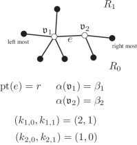
Figure 1. A boundary SD-ribbon tree

Definition .

We denote by

(2.15) $$\mathcal{M}^{\rm RGW}_{k_{1,1},k_{1,0}}(L_{1},L_{0};p,r;\beta_{1})\,\hat{\times}\,\mathcal{M}^{\rm RGW}_{k_{2,1},k_{2,0}}(L_{1},L_{0};r,q;\beta_{2})$$

the union of all moduli spaces ${\mathcal{M}}^{0}(\mathcal{R}^{\prime})$ such that:

$$\mathcal{R}^{\prime}\leq\mathcal{R}^{(1)}(p,r,q;\beta_{1},\beta_{2};k_{1,0},k_{1,1};k_{2,0},k_{2,1})$$

for some $r,\beta_{1},\beta_{2},k_{1,0},k_{1,1},k_{2,0},k_{2,1}$ as above.

By [part1:top, Theorem 4.61], (2.15) is closed in $\mathcal{M}^{\rm RGW}_{k_{1},k_{0}}(L_{1},L_{0};p,q;\beta)$. The arguments of [part2:kura] show that (2.15) has a Kuranishi structure and is a component of the normalized boundary of $\mathcal{M}^{\rm RGW}_{k_{1},k_{0}}(L_{1},L_{0};p,q;\beta)$.

Proposition .

Kuranishi structures of our moduli spaces can be chosen such that the following holds. There exists a continuous map:

$$\Pi: \mathcal{M}^{\rm RGW}_{k_{1,1},k_{1,0}}(L_{1},L_{0};p,r;\beta_{1})\,\hat{\times}\,\mathcal{M}^{\rm RGW}_{k_{2,1},k_{2,0}}(L_{1},L_{0};r,q;\beta_{2})$$

$$\to\mathcal{M}^{\rm RGW}_{k_{1,1},k_{1,0}}(L_{1},L_{0};p,r;\beta_{1})\times\mathcal{M}^{\rm RGW}_{k_{2,1},k_{2,0}}(L_{1},L_{0};r,q;\beta_{2})$$

with the following properties.

1. On the inverse image of the complement of

   (2.16) $$\left(\mathcal{M}^{\rm RGW}_{k_{1,1},k_{1,0}}(L_{1},L_{0};p,r;\beta_{1})^{(1)}\times\mathcal{M}^{\rm RGW}_{k_{2,1},k_{2,0}}(L_{1},L_{0};r,q;\beta_{2})\right)$$

   $$\cup\left(\mathcal{M}^{\rm RGW}_{k_{1,1},k_{1,0}}(L_{1},L_{0};p,r;\beta_{1})\times\mathcal{M}^{\rm RGW}_{k_{2,1},k_{2,0}}(L_{1},L_{0};r,q;\beta_{2})^{(1)}\right)$$

   $\Pi$ is induced by an isomorphism of Kuranishi structures.

2. Let $\mathfrak{p}$ be an element of

   (2.17) $$\mathcal{M}^{\rm RGW}_{k_{1,1},k_{1,0}}(L_{1},L_{0};p,r;\beta_{1})\,\hat{\times}\,\mathcal{M}^{\rm RGW}_{k_{2,1},k_{2,0}}(L_{1},L_{0};r,q;\beta_{2})$$

   and

   $$\overline{\mathfrak{p}}:=\Pi(\mathfrak{p})\in\mathcal{M}^{\rm RGW}_{k_{1,1},k_{1,0}}(L_{1},L_{0};p,r;\beta_{1})\times\mathcal{M}^{\rm RGW}_{k_{2,1},k_{2,0}}(L_{1},L_{0};r,q;\beta_{2}).$$

   Then the Kuranishi neighborhoods $\mathcal{U}_{\mathfrak{p}}=(U_{\mathfrak{p}},E_{\mathfrak{p}},s_{\mathfrak{p}},\psi_{\mathfrak{p}})$ and $\mathcal{U}_{\overline{\mathfrak{p}}}=(U_{\overline{\mathfrak{p}}},E_{\overline{\mathfrak{p}}},s_{\overline{\mathfrak{p}}},\psi_{\overline{\mathfrak{p}}})$ of $\mathfrak{p}$ and $\overline{\mathfrak{p}}$ assigned by our Kuranishi structures have the following properties. Let $U_{\mathfrak{p}}=V_{\mathfrak{p}}/\Gamma_{\mathfrak{p}}$ and $U_{\overline{\mathfrak{p}}}=V_{\overline{\mathfrak{p}}}/\Gamma_{\overline{\mathfrak{p}}}$.

   1. There exists an injective group homomorphism $\phi_{\mathfrak{p}}:\Gamma_{\mathfrak{p}}\to\Gamma_{\overline{\mathfrak{p}}}$.

   2. There exists a $\phi_{\mathfrak{p}}$-equivariant map

      $$F_{\mathfrak{p}}:V_{\mathfrak{p}}\to V_{\overline{\mathfrak{p}}}$$

      that is a strata-wise smooth submersion.

   3. $E_{\mathfrak{p}}$ is isomorphic to the pullback of $E_{\overline{\mathfrak{p}}}$ by $F_{\mathfrak{p}}$. In other words, there exists fiberwise isomorphic lift

      $$\tilde{F}_{\mathfrak{p}}:E_{\mathfrak{p}}\to E_{\overline{\mathfrak{p}}}$$

      of $F_{\mathfrak{p}}$, which is $\phi_{\mathfrak{p}}$ equivariant.

   4. $\tilde{F}_{\mathfrak{p}}\circ s_{\mathfrak{p}}=s_{\overline{\mathfrak{p}}}\circ F_{\mathfrak{p}}$.

   5. $\psi_{\overline{\mathfrak{p}}}\circ F_{\mathfrak{p}}=\Pi\circ\psi_{\mathfrak{p}}$ on $s_{\mathfrak{p}}^{-1}(0)$.

3. $\tilde{F}_{\mathfrak{p}},F_{\mathfrak{p}}$ are compatible with the coordinate changes.

Before turning to the proof of this proposition, we elaborate on Item (3). Recall that a Kuranishi structure for $X$ assigns a Kuranishi chart $\mathcal{U}_{\mathfrak{p}}=(U_{\mathfrak{p}},E_{\mathfrak{p}},s_{\mathfrak{p}},\psi_{\mathfrak{p}})$ to each $\mathfrak{p}\in X$. If $\mathfrak{q}\in{\rm Im}(\psi_{\mathfrak{p}})$, then we require that there exists a coordinate change $\Phi_{\mathfrak{p}\mathfrak{q}}=(U_{\mathfrak{p}\mathfrak{q}},\widehat{\varphi}_{\mathfrak{p}\mathfrak{q}},\varphi_{\mathfrak{p}\mathfrak{q}})$ from $\mathcal{U}_{\mathfrak{q}}$ to $\mathcal{U}_{\mathfrak{p}}$ in the following sense:

1. There exists an open neighborhood $U_{\mathfrak{p}\mathfrak{q}}$ of $o_{\mathfrak{q}}$ in $U_{\mathfrak{q}}$.

2. There exists an embedding of orbifolds $\varphi_{\mathfrak{p}\mathfrak{q}}:U_{\mathfrak{p}\mathfrak{q}}\to U_{\mathfrak{p}}$.

3. There exists an embedding of orbibundles $\widehat{\varphi}_{\mathfrak{p}\mathfrak{q}}:E_{\mathfrak{q}}|_{U_{\mathfrak{p}\mathfrak{q}}}\to E_{\mathfrak{p}}$ which is a lift of $\varphi_{\mathfrak{p}\mathfrak{q}}$.

4. $\widehat{\varphi}_{\mathfrak{p}\mathfrak{q}}$ is compatible with Kuranishi maps and parametrization maps in the following sense:

   1. $s_{\mathfrak{p}}\circ\varphi_{\mathfrak{p}\mathfrak{q}}=\widehat{\varphi}_{\mathfrak{p}\mathfrak{q}}\circ s_{\mathfrak{q}}$.

   2. $\psi_{\mathfrak{p}}\circ\varphi_{\mathfrak{p}\mathfrak{q}}=\psi_{\mathfrak{q}}$ on $U_{\mathfrak{p}\mathfrak{q}}\cap s_{\mathfrak{q}}^{-1}(0)$.

5. On ${\rm Im}(\varphi_{\mathfrak{p}\mathfrak{q}})\cap s_{\mathfrak{p}}^{-1}(0)$, the differential $ds_{\mathfrak{p}}$ induces a bundle isomorphism:

   $$\mathcal{N}_{U_{\mathfrak{p}\mathfrak{q}}}U_{\mathfrak{p}}\cong\frac{E_{\mathfrak{p}}}{{\rm Im}(\widehat{\varphi}_{\mathfrak{p}\mathfrak{q}})}.$$

   where the bundle on the left hand side denotes the normal bundle of $\varphi_{\mathfrak{p}\mathfrak{q}}(U_{\mathfrak{p}\mathfrak{q}})$ in $U_{\mathfrak{p}}$.

See [fooobook2, Definition A.1.3 and Definition A1.14] or [fooonewbook, Definition 3.6]. The notion of embedding of orbifolds and orbibundle is defined in [fooonewbook, Chapter 23]. The coordinate change maps $\Phi_{\mathfrak{p}\mathfrak{q}}$ are required to satisfy certain compatibility conditions and we refer the reader to [fooobook2, (A1.6.2)], [fooonewbook, Definition 3.9] for these conditions.

In Proposition 2.2, let $\mathfrak{p}$, $\mathfrak{q}$ be elements of (2.17) such that $\mathfrak{q}\in{\rm Im}(\psi_{\mathfrak{p}})$. We denote $\Pi(\mathfrak{p})$, $\Pi(\mathfrak{q})$ by $\overline{\mathfrak{p}}$, $\overline{\mathfrak{q}}$. We then have $\varphi_{\mathfrak{p}\mathfrak{q}}$, $\widehat{\varphi}_{{\mathfrak{p}}{\mathfrak{q}}}$, $\varphi_{\overline{\mathfrak{p}}\overline{\mathfrak{q}}}$, $\widehat{\varphi}_{\overline{\mathfrak{p}}\overline{\mathfrak{q}}}$. Item (3) of Proposition 2.2 asserts that:

$$F_{\mathfrak{p}}\circ\varphi_{\mathfrak{p}\mathfrak{q}}=\varphi_{\overline{\mathfrak{p}}\overline{\mathfrak{q}}}\circ F_{\mathfrak{q}},\qquad\widetilde{F}_{\mathfrak{p}}\circ\widehat{\varphi}_{{\mathfrak{p}}{\mathfrak{q}}}=\widehat{\varphi}_{\overline{\mathfrak{p}}\overline{\mathfrak{q}}}\circ\widetilde{F}_{\mathfrak{q}}$$

on the domain where both sides are defined.

Proof of Proposition 2.2.

We construct the continuous map $\Pi$ in this subsection. The study of its relation to Kuranishi structure is postponed to Section 3.

Removing the edge $e$ of $\mathcal{R}=\mathcal{R}^{(1)}(p,r,q;\beta_{1},\beta_{2};k_{1,0},k_{1,1};k_{2,0},k_{2,1})$ and adding two exterior vertices produces two SD-ribbon graphs $\mathcal{R}_{1}$, $\mathcal{R}_{2}$ of types $(p,r;\beta_{1};k_{1,0},k_{1,1})$, $(r,q;\beta_{2};k_{2,0},k_{2,1})$. (See Figure 2.) Let $\mathcal{R}^{\prime}_{1}$ (resp. $\mathcal{R}^{\prime}_{2}$) be an SD-ribbon tree of type $(p,r;\beta_{1};k_{1,0},k_{1,1})$ (resp. $(r,q;\beta_{2};k_{2,0},k_{2,1})$) such that $\mathcal{R}^{\prime}_{1}\leq\mathcal{R}_{1}$ (resp. $\mathcal{R}^{\prime}_{2}\leq\mathcal{R}_{2}$). We glue the edge incident to the right most vertex of $\mathcal{R}^{\prime}_{1}$ to the edge incident to the left most vertex of $\mathcal{R}^{\prime}_{2}$. (The right most vertex of $\mathcal{R}^{\prime}_{1}$ and the left most vertex of $\mathcal{R}^{\prime}_{2}$ are not vertices of the resulting tree.)

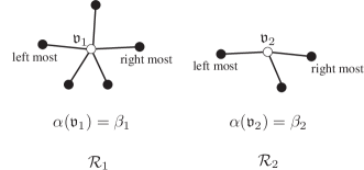
Figure 2. $\mathcal{R}_{1}$ and $\mathcal{R}_{2}$.

This tree together with a level function determines an SD-ribbon tree of type $(\beta,k_{0},k_{1})$. Let $\hat{\lambda}$ be a level function associated to a quasi order $\leq$, which restricts to the quasi order associated to $\mathcal{R}^{\prime}_{i}$ on $C^{\rm ins}_{0}(\hat{R}^{\prime}_{i})$. Note that the choice of $\hat{\lambda}$ is not unique. (See Figure 3.) We denote the resulting SD-ribbon tree of type $(\beta;k_{0},k_{1})$ by:

$$\mathcal{R}^{\prime}_{1}\#_{\hat{\lambda}}\mathcal{R}^{\prime}_{2}$$

For any SD-ribbon tree $\mathcal{R}^{\prime}$ of type $(\beta;k_{0},k_{1})$ with $\mathcal{R}^{\prime}\leq\mathcal{R}$, there exist unique $\mathcal{R}^{\prime}_{1}$, $\mathcal{R}^{\prime}_{2}$ and $\hat{\lambda}$ such that:

(2.18) $$\mathcal{R}^{\prime}=\mathcal{R}^{\prime}_{1}\#_{\hat{\lambda}}\mathcal{R}^{\prime}_{2}.$$

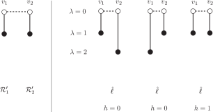
Figure 3. Three different choices of $\hat{\ell}$.

For $\mathcal{R}^{\prime}$ as in (2.18), the map $\Pi$ restricts to a map:

$$\Pi:{\mathcal{M}}^{0}(\mathcal{R}^{\prime})\to{\mathcal{M}}^{0}(\mathcal{R}^{\prime}_{1})\times{\mathcal{M}}^{0}(\mathcal{R}^{\prime}_{2}).$$

which can be described as follows. Let $|\hat{\lambda}|$, $|\lambda_{1}|$ and $|\lambda_{2}|$ be the number of positive levels of $\mathcal{R}^{\prime}$, $\mathcal{R}_{1}^{\prime}$ and $\mathcal{R}_{2}^{\prime}$. The fact that the quasi order corresponding to $\hat{\lambda}$ restricts to the quasi order corresponding $\lambda_{i}$ on $C^{\rm ins}_{0}(\hat{R}_{i})$ implies that $|\hat{\lambda}|\leq|\lambda_{1}|+|\lambda_{2}|$. Let $h=|\lambda_{1}|+|\lambda_{2}|-|\hat{\lambda}|$. Using identifications:

$$\widetilde{\mathcal{M}}^{0}(\mathcal{R}^{\prime}_{1})\times\widetilde{\mathcal{M}}^{0}(\mathcal{R}^{\prime}_{2})=\widetilde{\mathcal{M}}^{0}(\mathcal{R}^{\prime}),\hskip 28.45274pt{\rm Aut}(\mathcal{R}^{\prime})={\rm Aut}(\mathcal{R}^{\prime}_{1})\times{\rm Aut}(\mathcal{R}^{\prime}_{2}),$$

it is easy to see that there exists a ${\mathbb{C}}_{*}^{h}$-action on ${\mathcal{M}}^{0}(\mathcal{R}^{\prime})$ such that

(2.19) $${\mathcal{M}}^{0}(\mathcal{R}^{\prime}_{1})\times{\mathcal{M}}^{0}(\mathcal{R}^{\prime}_{2})={\mathcal{M}}^{0}(\mathcal{R}^{\prime})/{\mathbb{C}}_{*}^{h}.$$

The map $\Pi$ is defined to be the projection map induced by this identification. ∎

We thus gave a detailed description of the part of the boundary of the moduli space $\mathcal{M}^{\rm RGW}_{k_{1},k_{0}}(L_{1},L_{0};p,q;\beta)$ given in Definition 2.2. Next, we describe other boundary elements in a similar way.

Definition .

A boundary SD-ribbon trees of type (2) for $\mathcal{M}^{\rm RGW}_{k_{1},k_{0}}(L_{1},L_{0};p,q;\beta)$ is an SD-ribbon tree

$$\mathcal{R}^{(2)}(p,q;\beta_{1},\beta_{2};k_{1,1}+1,k_{2,1},j;k_{0})=(R;\mathfrak{v}_{l},\mathfrak{v}_{r};\mathcal{S},{\rm pt},\alpha,\leq)$$

where $\beta_{1}\in\Pi_{2}(L_{1},L_{0};p,q)$, $\beta_{2}\in\Pi_{2}(X,L_{1})$, $\beta=\beta_{1}\#\beta_{2}$, $k_{1,1}+k_{2,1}=k_{1}$ and $j\in\{1,\dots,k_{1,1}+1\}$. This SD-ribbon tree is required to satisfy the following properties:

• There are only two interior vertices $\mathfrak{v}_{1}$ and $\mathfrak{v}_{2}$. The vertex $\mathfrak{v}_{1}$ has color ${\rm str}$ and $\mathfrak{v}_{2}$ has color ${\rm d_{1}}$. There is an edge $e$ connecting $\mathfrak{v}_{1}$ to $\mathfrak{v}_{2}$.

• The graphs $R_{1}$ has exactly $k_{1,1}+1$ exterior vertices connected to $\mathfrak{v}_{1}$ and $k_{2,1}$ exterior vertices connected to $\mathfrak{v}_{2}$. The edge $e$ is the $j$-th edge in $R_{1}$ connected to $\mathfrak{v}_{1}$. Here we use the ribbon structure at $\mathfrak{v}_{1}$ to label the edges in $R_{1}$, which are connected to $\mathfrak{v}_{1}$. The graph $R_{0}$ has only $k_{0}$ exterior vertices connected to $\mathfrak{v}_{1}$.

• $\mathcal{S}(\mathfrak{v}_{1})$ (resp. $\mathcal{S}(\mathfrak{v}_{2})$) is the unique SD-tree (resp. DD-tree) of type $(p,q;\beta_{1};k_{0},k_{1,1}+1)$ (resp. $(\beta_{2};k_{2,1})$) with only one vertex (which is necessarily labeled with d).

We can similarly define boundary SD-ribbon trees of type (3), which have the form:

$$\mathcal{R}^{(3)}(p,q;\beta_{1},\beta_{2};k_{1};k_{1,0};k_{2,0}+1,j).$$

Figure 4 gives examples of boundary SD-ribbon trees of types (2) and (3).

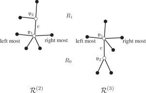
Figure 4. The ribbon trees $\mathcal{R}^{(2)}$ and $\mathcal{R}^{(3)}$

Definition .

We define

(2.20) $$\mathcal{M}^{\rm RGW}_{k_{1,1}+1,k_{0}}(L_{1},L_{0};p,q;\beta_{1})\,{}_{{\rm ev}_{1,j}}\hat{\times}_{{\rm ev_{0}}}\,\mathcal{M}^{\rm RGW}_{k_{2,1}+1}(L_{1};\beta_{2})$$

to be the union of all ${\mathcal{M}}^{0}(\mathcal{R}^{\prime})$ with $\mathcal{R}^{\prime}\leq\mathcal{R}^{(2)}(p,q;\beta_{1},\beta_{2};k_{1,1}+1,k_{2,1},j;k_{0})$. Similarly, we define

(2.21) $$\mathcal{M}^{\rm RGW}_{k_{1},k_{1,0}+1}(L_{1},L_{0};p,q;\beta_{1})\,{}_{{\rm ev}_{0,j}}\hat{\times}_{{\rm ev_{0}}}\,\mathcal{M}^{\rm RGW}_{k_{2,0}+1}(L_{0};\beta_{2}).$$

Proposition .

There exists a map

(2.22) $$\Pi: \mathcal{M}^{\rm RGW}_{k_{1,1}+1,k_{0}}(L_{1},L_{0};p,q;\beta_{1})\,{}_{{\rm ev}_{1,j}}\hat{\times}_{{\rm ev_{0}}}\,\mathcal{M}^{\rm RGW}_{k_{2,1}+1}(L_{1};\beta_{2})$$

$$\to\mathcal{M}^{\rm RGW}_{k_{1,1}+1,k_{0}}(L_{1},L_{0};p,q;\beta_{1})\,{}_{{\rm ev}_{1,j}}\times_{{\rm ev_{0}}}\,\mathcal{M}^{\rm RGW}_{k_{2,1}+1}(L_{1};\beta_{2})$$

satisfying the following properties.

1. On the inverse image of the complement of

   $$\left(\mathcal{M}^{\rm RGW}_{k_{1,1},k_{0}}(L_{1},L_{0};p,q;\beta_{1})^{(1)}\right)\,{}_{{\rm ev}_{1,j}}\times_{{\rm ev_{0}}}\,\left(\mathcal{M}^{\rm RGW}_{k_{2,1}+1}(L_{1};\beta_{2})\right)$$

   $$\cup\left(\mathcal{M}^{\rm RGW}_{k_{1,1},k_{0}}(L_{1},L_{0};p,q;\beta_{1})\right)\,{}_{{\rm ev}_{1,j}}\times_{{\rm ev_{0}}}\,\left(\mathcal{M}^{\rm RGW}_{k_{2,1}+1}(L_{1};\beta_{2})^{(1)}\right)$$

   $\Pi$ is induced by the isomorphism of Kuranishi structures. Here the fiber product is taken over $L_{1}$.

2. The same property as in Proposition 2.2 (2) holds.

3. The same property as in Proposition 2.2 (3) holds.

A similar statement holds for:

$$\mathcal{M}^{\rm RGW}_{k_{1},k_{1,0}}(L_{1},L_{0};p,q;\beta_{1})\,{}_{{\rm ev}_{0,j}}\hat{\times}_{{\rm ev_{0}}}\,\mathcal{M}^{\rm RGW}_{k_{2,0}+1}(L_{0};\beta_{2}).$$

The proof is similar to the proof of Proposition 2.2 and is omitted.

Proposition .

The normalized boundary of $\mathcal{M}^{\rm RGW}_{k_{1},k_{0}}(L_{1},L_{0};p,q;\beta)$ is the disjoint union of (2.15), (2.20), (2.21).

Proof.

By the calculation of dimension we gave in the proof of Proposition 2.2, the only codimension 1 strata are $\mathcal{R}^{(1)}(p,r,q;\beta_{1},\beta_{2};k_{1,0},k_{1,1};k_{2,0},k_{2,1})$, $\mathcal{R}^{(2)}(p,q;\beta_{1},\beta_{2};k_{1,1}+1,k_{2,1},j;k_{0})$ and $\mathcal{R}^{(3)}(p,q;\beta_{1},\beta_{2};k_{1};k_{1,0};k_{2,0}+1,j)$. This gives the lemma. ∎

2.3. Construction of multisection

In this subsection, we prove Theorem 2.1. The proof is by induction on $\omega\cap\beta$ and $(k_{0},k_{1})$. In this inductive process we construct multi-valued perturbations for all moduli spaces $\omega\cap\beta\leq E$ and $k_{0}+k_{1}\leq N$ for some constants $E$ and $N$. In particular, we may construct perturbations for the moduli spaces with dimension greater than $1$. But the conditions (1) and (3) hold only for moduli spaces with dimension at most $1$. We assume that we already constructed multi-valued perturbations for the moduli spaces of type $(\beta;k_{0},k_{1};p,q)$ such that $\omega\cap\beta<\omega\cap\alpha$ or $\omega\cap\beta=\omega\cap\alpha$ and $k_{1}+k_{1}<j_{1}+j_{2}$.

We fix a continuous multi-section on $\partial\mathcal{M}^{\rm RGW}_{j_{1},j_{0}}(L_{1},L_{0};p,q;\alpha)$ using the induction hypothesis. For example, part of the boundary of the moduli space $\mathcal{M}^{\rm RGW}_{j_{1},j_{0}}(L_{1},L_{0};p,q;\alpha)$ is described by the moduli spaces of the form

(2.23) $$\mathcal{M}^{\rm RGW}_{j_{1}^{\prime},j_{0}}(L_{1},L_{0};p,q;\beta_{1})\hat{\times}_{L_{1}}\mathcal{M}^{\rm RGW}_{j_{1}^{\prime\prime}+1}(L_{1};\beta_{2}),$$

where $j_{1}^{\prime}+j_{1}^{\prime\prime}=j_{1}+1$, $\beta_{i}\cap\mathcal{D}=0$ and $\beta_{1}\#\beta_{2}=\alpha$. Assuming $\mathcal{M}^{\rm RGW}_{k_{1}^{\prime\prime}+1}(L_{1};\beta_{2})$ is non-empty, we have $\omega\cap\beta_{1}<\omega\cap\alpha$ or $j_{1}^{\prime}<j_{1}$ and $\omega\cap\beta_{1}\leq\omega\cap\alpha$ . Therefore, the induction hypothesis implies that we already fixed a multi-valued perturbation for $\mathcal{M}^{\rm RGW}_{j_{1}^{\prime},j_{0}}(L_{1},L_{0};p,q;\beta_{1})$. We use the fiber product of this perturbation and the trivial perturbation for $\mathcal{M}^{\rm RGW}_{j_{1}^{\prime\prime}+1}(L_{1};\beta_{2})$ to define a multi-valued perturbation for:

$$\mathcal{M}^{\rm RGW}_{j_{1}^{\prime},j_{0}}(L_{1},L_{0};p,q;\beta_{1})\times_{L_{1}}\mathcal{M}^{\rm RGW}_{j_{1}^{\prime\prime}+1}(L_{1};\beta_{2})$$

Now we use the map $\Pi$ in Proposition 2.2 to pull-back this perturbation to the space in (2.23). More generally, we can use the already constructed perturbations for the moduli spaces of strips and trivial perturbations for the moduli spaces of discs to define a multi-valued perturbation for any boundary component and corner of $\mathcal{M}^{\rm RGW}_{j_{1},j_{0}}(L_{1},L_{0};p,q;\alpha)$. The induction hypothesis implies that these perturbations are compatible.

In the case that the virtual dimension of $\mathcal{M}^{\rm RGW}_{j_{1},j_{0}}(L_{1},L_{0};p,q;\alpha)$ is greater than $1$, we extend the chosen multi-valued perturbation on the boundary into a $C^{0}$ perturbation defined over the whole moduli space. In the case that the virtual dimension is at most $1$, we need to choose this extension such that the conditions in (1) and (3) of Theorem 2.1 are satisfied. To achieve this goal, we analyze the vanishing locus of the multi-valued perturbation over the boundary of $\mathcal{M}^{\rm RGW}_{j_{1},j_{0}}(L_{1},L_{0};p,q;\alpha)$.

Let $\mathcal{M}^{\rm RGW}_{j_{1},j_{0}}(L_{1},L_{0};p,q;\alpha)$ have virtual dimension not greater than $1$. On the stratum of the boundary where there exists at least one disk bubble on which the map is non-constant, the assumption implies that the Maslov number of the disk bubble is at least $4$. This implies that there is at least one irreducible component, which is a strip with homology class $\beta_{1}$ and is contained in a moduli space with negative virtual dimension. Therefore, our multi-valued perturbation on this boundary component does not vanish.

The rest of the proof is divided into two parts. We firstly consider the case where $\dim(\mathcal{M}^{\rm RGW}_{j_{1},j_{0}}(L_{1},L_{0};p,q;\alpha))$ is non-positive. The part of the boundary corresponding to splitting into two or more strips has a strip component which has negative virtual dimension. Therefore, our multi-valued perturbation does not vanish on this part of the boundary, too. As a consequence, we can extend the perturbation in the $C^{0}$ sense to a neighborhood of the boundary such that it is still non-vanishing in this neighborhood. We approximate the perturbation by a section which is $C^{1}$ outside a smaller neighborhood of the boundary. Now we can extend this multi-section in a way which is transversal to $0$ on $\mathcal{M}^{\rm RGW}_{k_{1},k_{0}}(L_{1},L_{0};p,q;\beta)$ and $\mathcal{M}^{\rm RGW}_{k_{1},k_{0}}(L_{1},L_{0};p,q;\beta)^{(1)}$ using the existence theorem of multi-valued perturbations. (See, for example, [fooonewbook, Theorem 13.5].) If the virtual dimension is $0$, there exists finitely many zeros which do not belong to $\mathcal{M}^{\rm RGW}_{k_{1},k_{0}}(L_{1},L_{0};p,q;\beta)^{(1)}$. If the virtual dimension is negative, the multi-valued perturbation does not vanish. This completes the proof in the case that $\dim(\mathcal{M}^{\rm RGW}_{j_{1},j_{0}}(L_{1},L_{0};p,q;\alpha))\leq 0$.

Next, we consider the case that $\mathcal{M}^{\rm RGW}_{j_{1},j_{0}}(L_{1},L_{0};p,q;\alpha)$ is $1$-dimensional. The constructed multi-valued perturbation on the boundary does not vanish except on the boundary components of the form

(2.24) $$\mathcal{M}^{\rm RGW}_{j^{\prime}_{1},j^{\prime}_{0}}(L_{1},L_{0};p,r;\beta_{1})\hat{\times}\mathcal{M}^{\rm RGW}_{j^{\prime\prime}_{1},j^{\prime\prime}_{0}}(L_{1},L_{0};r,q;\beta_{2}),$$

or

(2.25) $$\mathcal{M}^{\rm RGW}_{j_{1}-1,j_{0}}(L_{1},L_{0};p,q;\alpha)\hat{\times}_{L_{1}}\mathcal{M}^{\rm RGW}_{3}(L_{1};0),$$

$$\mathcal{M}^{\rm RGW}_{j_{1},j_{0}-1}(L_{1},L_{0};p,q;\alpha)\hat{\times}_{L_{0}}\mathcal{M}^{\rm RGW}_{3}(L_{0};0).$$

In (2.24), both of the factors have virtual dimension $0$. Therefore, we may assume that the zero set of the multi-valued perturbation we have defined on those factors do not lie in the strata of codimension at least $2$. Since the multi-sections on the two factors have finitely many zeros and the map $\Pi$ in Proposition 2.2 is an isomorphism, the first factor gives rise to finitely many points in the boundary. In the case of (2.25), the first factor has virtual dimension $0$ and the multi-section there vanishes only at finitely many points. The second factor is identified with $L_{1}$ or $L_{0}$. Therefore, the fiber product is identified with the first factor. In summary, the multi-valued perturbation has finitely many zeros on the boundary and item (3) holds.

We fix Kuranishi charts at the finitely many zeros on the boundary. Since these are boundary points, we can easily extend our multi-valued perturbation to the interior of the chosen Kuranishi charts so that it is transversal to $0$. Now we extend the multi-valued perturbation further to a neighborhood of the boundary of $\mathcal{M}^{\rm RGW}_{j_{1},j_{0}}(L_{1},L_{0};p,q;\alpha)$ in the $C^{0}$ sense such that the multi-valued perturbation does not vanish except at those finitely many charts. We may assume that the multi-valued perturbation is $C^{1}$ outside a smaller neighborhood of the boundary. We use again the existence theorem of multi-sections that are transversal to zero everywhere to complete the construction of the multi-valued perturbation on $\mathcal{M}^{\rm RGW}_{j_{1},j_{0}}(L_{1},L_{0};p,q;\alpha)$. ∎

Remark .

This proof never uses the smoothness of the coordinate change with respect to the gluing parameters $\sigma_{e}$ when $\sigma_{e}=0$. In most part of the proof, we extend the multi-section at the boundary to the interior only in the $C^{0}$ sense. When we extend the multi-section near a point of the boundary where it vanishes, we fix a chart there and extend it on that chart. We use other charts to extend the multi-section in $C^{0}$ sense to a neighborhood of the boundary. (Recall that we only need the differentiability of the multi-valued perturbation in a neighborhood of its vanishing set to define virtual fundamental chain.) The key point here is that the multi-valued perturbation on the boundary has only isolated zeros.

Remark .

Even though we do not perturb the moduli spaces of disks of virtual dimension greater than $1$ in the proof of Theorem 2.1, we used the fact that these moduli spaces admit Kuranishi structures.

2.4. Completion of the proof of Theorem 2.1

We consider $p,q\in L_{0}\cap L_{1}$ and $\beta\in\Pi_{2}(L_{1},L_{0};p,q)$ such that

$$\dim\mathcal{M}^{\rm RGW}_{0,0}(L_{1},L_{0};p,q;\beta)=1.$$

By Corollary 2.1 (3), we have

(2.26) $$[\partial\mathcal{M}^{\rm RGW}_{0,0}(L_{1},L_{0};p,q;\beta),\widehat{\mathfrak{s}}^{n}]=0.$$

We will prove that the sum of (2.26) over all possible choices of $\beta$ becomes the coefficient of $[q]$ in $\partial\circ\partial([p])$, which will show that $\partial$ is a differential.

We study various types of boundary elements appearing in Theorem 2.1. The contribution of the elements in part (1) of Theorem 2.1 is given as

(2.27) $$[(\mathcal{M}^{\rm RGW}_{0,0}(L_{1},L_{0};p,r;\beta_{1})\hat{\times}\mathcal{M}^{\rm RGW}_{0,0}(L_{1},L_{0};r,q;\beta_{2}),\widehat{\mathfrak{s}}^{n})].$$

We claim that this is equal to

(2.28) $$[(\mathcal{M}^{\rm RGW}_{0,0}(L_{1},L_{0};p,r;\beta_{1}),\widehat{\mathfrak{s}}^{n})][(\mathcal{M}^{\rm RGW}_{0,0}(L_{1},L_{0};r,q;\beta_{2}),\widehat{\mathfrak{s}}^{n})].$$

The number $[(\mathcal{M}^{\rm RGW}_{0,0}(L_{1},L_{0};p,r;\beta_{1}),\widehat{\mathfrak{s}}^{n})]$ is a weighted count of the zeroes of $\mathfrak{s}^{n}$ on this moduli space. By Theorem 2.1 (3), this zero set is disjoint from $\mathcal{M}^{\rm RGW}_{0,0}(L_{1},L_{0};p,r;\beta_{1})^{(1)}$. The same conclusion holds for the virtual chain $[(\mathcal{M}^{\rm RGW}_{0,0}(L_{1},L_{0};r,q;\beta_{2}),\widehat{\mathfrak{s}}^{n})]$. Therefore, the map $\Pi$ in (2.22) induces an isomorphism of Kuranishi structures on a neighborhood of the zero set of $\widehat{\mathfrak{s}}^{n}$. It follows that the weighted count of (2.27) is equal to (2.28). To complete the proof of Theorem 2.1, it suffices to show the contribution of the other boundary components vanishes.

We firstly consider the contribution from Item (2) of Theorem 2.1, which is

(2.29) $$\mathcal{M}^{\rm RGW}_{0,1}(L_{1},L_{0};p,q;\beta^{\prime})\,\hat{\times}_{L_{0}}\,\mathcal{M}^{\rm RGW}_{1}(L_{0};\alpha).$$

If $\mathcal{M}^{\rm RGW}_{1}(L_{0};\alpha)$ is nonempty, then $\omega(\alpha)>0$. Using monotonicity and the fact that the minimum Maslov number of $L_{0}$ is at least $4$, we can conclude that $\mu(\alpha)\geq 4$. This inequality together with $\mu(\beta)=2$ implies that $\mu(\beta^{\prime})\leq-2$. Thus the moduli space $\mathcal{M}^{\rm RGW}_{0,1}(L_{1},L_{0};p,q;\beta^{\prime})$ has a negative dimension. By Corollary 2.1, $\widehat{\mathfrak{s}}^{n}$ never vanishes on $\mathcal{M}^{\rm RGW}_{0,1}(L_{1},L_{0};p,q;\beta^{\prime})$. Therefore, (2.29) is empty after the perturbation given by $\widehat{\mathfrak{s}}^{n}$, and hence it does not contribute to (2.26). In the same way, we can show Item (3) of Theorem 2.1 does not contribute to (2.26). This completes the proof of Theorem 2.1, except that we still need to construct Kuranishi structures required for Propositions 2.2, 2.2, 2.2 which will be done in Section 3. ∎

Definition .

If Condition 2.1 is satisfied, then we define the Lagrangian Floer homology of $L_{0}$ and $L_{1}$ as

$$HF(L_{1},L_{0};o;X\setminus\mathcal{D})\cong\frac{{\rm Ker}\left(\partial:CF(L_{1},L_{0};{\mathbb{Q}};o)\to CF(L_{1},L_{0};{\mathbb{Q}};o)\right)}{{\rm Im}\left(\partial:CF(L_{1},L_{0};{\mathbb{Q}};o)\to CF(L_{1},L_{0};{\mathbb{Q}};o)\right)}.$$

We remark that Item (1) of Theorem 2.1,

$${\rm rank}HF(L_{1},L_{0};o;X\setminus\mathcal{D})\leq\#L_{0}\cap_{o}L_{1},$$

is immediate from the definition.

3. Construction of a System of Kuranishi Structures

3.1. Statement

In [part2:kura], we constructed a Kuranishi structure for each moduli space $\mathcal{M}_{k+1}^{\rm RGW}(L;\beta)$. In this section, we study how these Kuranishi structures are related to each other at their boundaries and corners. More specifically, we prove the disk moduli version of Propositions 2.2, 2.2, 2.2, stated as Theorem 3.1. The notation $\hat{\times}_{L}$ is discussed in Subsection 2.2. Recall also from Subsection 2.2 that $\mathcal{M}^{\rm RGW}_{k_{1}+1}(L;\beta_{1})^{(1)}$ is the union of the strata of $\mathcal{M}_{k+1}^{\rm RGW}(L;\beta)$ which are described by DD-ribbon trees with at least one positive level. The proof of Propositions 2.2, 2.2, 2.2 is similar to that of Theorem 3.1. Thus, we only focus on the proof of Theorem 3.1.

Theorem .

Suppose $E$ is a positive real number and $N$ is a positive integer. There is a system of Kuranishi structures on the moduli spaces $\{\mathcal{M}^{\rm RGW}_{k+1}(L;\beta)\}_{k,\beta}$ with $\omega\cap\beta\leq E$ and $k\leq N$ such that if $\beta_{1}+\beta_{2}=\beta$, $k_{1}+k_{2}=k$, then the space

$$\mathcal{M}^{\rm RGW}_{k_{1}+1}(L;\beta_{1})\,\hat{\times}_{L}\,\mathcal{M}^{\rm RGW}_{k_{2}+1}(L;\beta_{2})$$

is a codimension one stratum of $\mathcal{M}^{\rm RGW}_{k+1}(L;\beta)$ with the following properties. There exists a continuous map

(3.1) $$\Pi: \mathcal{M}^{\rm RGW}_{k_{1}+1}(L;\beta_{1})\,\hat{\times}_{L}\,\mathcal{M}^{\rm RGW}_{k_{2}+1}(L;\beta_{2})$$

$$\to\mathcal{M}^{\rm RGW}_{k_{1}+1}(L;\beta_{1})\,\times_{L}\,\mathcal{M}^{\rm RGW}_{k_{2}+1}(L;\beta_{2})$$

which has the same properties as Proposition 2.22 (1),(2) and (3).

The proof of Theorem 3.1 occupies the rest of this section. For the proof, first we formulate the notion of obstruction bundle data in Definition 3.2. It is a way to associate an obstruction bundle to a neighborhood of each element of the moduli space. In [part2:kura], we defined and used a version of such obstruction bundle data. For the proof of Theorem 3.1, we need to slightly modify our choices of obstruction bundles so that they satisfy certain compatibility conditions at the boundary and corners. The notion of obstruction bundle data is introduced to state the required compatibility condition in a precise was as Definition 3.2 (disk-component-wise-ness). Then the proof of Theorem 3.1 is divided into two parts. We first show that the system of Kuranishi structures induced from a system of disk-component-wise obstruction bundle data has the property stated in Theorem 3.1. We then show the existence of disk-component-wise obstruction bundle data.

Remark .

Theorem 3.1 concerns only the behavior of Kuranishi structures at codimension one boundary components. In fact, there is a similar statement for the behavior of our Kuranishi structures at higher co-dimensional corners. This generalization to higher co-dimensional corners are counterparts of [fooonewbook, Condition 16.1 X, XI, XII] in the context of the stable map compactification. The main difference is that we need to replace $\times_{L}$ with $\hat{\times}_{L}$. To work out the whole construction of simultaneous perturbations, we need the generalization of Theorem 3.1 to the higher co-dimensional corners.

In Subsection 3.2, we will formulate a condition (Definition 3.2) for the obstruction spaces, which implies the consistency of Kuranishi structures at the corners of arbitrary codimension. Since the proof and the statement for the case of corners is a straightforward generalization of the case of boundary (but cumbersome to write in detail), we focus on the case of codimension one boundary components.

Remark .

The proof in this section is different from the approach in [fooo:const2, Section 8], where the case of stable map compactification is treated. In this section, we use target parallel transportation. On the other hand, in [fooo:const2, Section 8] extra marked points are added to $\mathfrak{p}\in\mathfrak{P}(k+1,\beta)$ and are used to fix a diffeomorphism between open subsets of the source domains.

3.2. Disk component-wise-ness of the Obstruction Bundle Data

A disk splitting tree is defined to be a very detailed DD-ribbon tree $\mathcal{S}$ such that the color of all vertices is ${\rm d}$. We say a detailed DD-ribbon tree $\check{R}$ belongs to a disk splitting tree $\mathcal{S}$ if $\mathcal{S}$ is obtained from $\check{R}$ by level shrinking and fine edge shrinking. (See [part2:kura, Section 8] for the definition of these combinatorial objects and operations.) In other words, geometrical objects with combinatorial type $\check{R}$ are limits of objects with type $\mathcal{S}$ such that new disc bubble does not occur. However, it is possible to have sphere bubbles.

Let $\mathfrak{u}\in\mathcal{M}^{\rm RGW}_{k+1}(L;\beta)$ and $\check{R}$ be the associated very detailed tree. Suppose $\mathcal{S}$ is a disk splitting tree such that $\check{R}$ belongs to $\mathcal{S}$. Let also $\lambda$ be the level function assigned to $\check{R}$. For each interior vertex $\mathfrak{v}$ of $\mathcal{S}$, let $\check{R}_{\mathfrak{v}}$ be the subtree of $\check{R}$ given by the connected component of

$$\check{R}\setminus\bigcup_{e\in C^{\rm int}_{1}({\check{R}}),\,\lambda(e)=0}e$$

which contains the vertex $\mathfrak{v}$. Let $\overline{\mathcal{S}}$ be a disk splitting tree obtained from $\mathcal{S}$ by a sequence of shrinking of level $0$ edges [part1:top, Definition 3.104]. Let $\pi:\mathcal{S}\to\overline{\mathcal{S}}$ be the associated contraction map. For each $\mathfrak{w}\in C^{\rm int}_{0}(\overline{\mathcal{S}})$, let ${\check{R}}(\mathfrak{w})$ be the very detailed DD-ribbon tree defined as

(3.2) $${\check{R}}(\mathfrak{w})=\bigcup_{\pi(\mathfrak{v})=\mathfrak{w}}\check{R}_{\mathfrak{v}}\cup\bigcup_{\begin{subarray}{c}e\in C^{\rm int}_{1}({\check{R}}),\,\lambda(e)=0,\\ \,\text{$\pi(e)$ is adjacent to $\mathfrak{w}$}\end{subarray}}e.$$

Clearly we have $C^{\rm int}_{0}({\check{R}}(\mathfrak{w}))\subseteq C^{\rm int}_{0}({\check{R}})$ and $C^{\rm int}_{1}({\check{R}}(\mathfrak{w}))\subseteq C^{\rm int}_{1}({\check{R}})$.

The restriction of the quasi-order of $C^{\rm int}_{0}({\check{R}})$ to the set $C^{\rm int}_{0}({\check{R}}(\mathfrak{w}))$ determines a level function $\lambda_{\mathfrak{w}}$ for ${\check{R}}(\mathfrak{w})$. The tree ${\check{R}}(\mathfrak{w})$ also inherits a multiplicity function, a homology class assigned to each interior vertex and a color function from $\check{R}$, which turn ${\check{R}}(\mathfrak{w})$ into a very detailed tree associated to a detailed DD-ribbon tree $\mathcal{R}(\mathfrak{w})$. There is a map

(3.3) $$\pi_{\mathfrak{w}}:\{1,\dots,|\lambda|\}\to\{1,\dots,|\lambda_{\mathfrak{w}}|\}$$

such that $i\leq j$ implies $\pi_{\mathfrak{w}}(i)\leq\pi_{\mathfrak{w}}(j)$ and for any $v\in C^{\rm int}_{0}({\mathcal{R}}(\mathfrak{w}))\subseteq C^{\rm int}_{0}({\mathcal{R}})$

(3.4) $$\lambda_{\mathfrak{w}}(v)=\pi_{\mathfrak{w}}(\lambda(v)).$$

Let $\Sigma_{\mathfrak{u}}$ be the source curve of $\mathfrak{u}$, and $\Sigma_{\mathfrak{u},v}$ denote the irreducible component of $\Sigma_{\mathfrak{u}}$ corresponding to an interior vertex $v$ of $\check{R}$. For any $\mathfrak{w}\in C^{\rm int}_{0}(\overline{\mathcal{S}})$, we define $\Sigma_{\mathfrak{u},\mathfrak{w}}$ to be the union of irreducible components $\Sigma_{\mathfrak{u},v}$ where $v\in C^{\rm int}_{0}({\check{R}}(\mathfrak{w}))$. A boundary marked point of $\Sigma_{\mathfrak{u},\mathfrak{w}}$ is either a boundary marked point of a disc component $\Sigma_{\mathfrak{u},v}$ in $\Sigma_{\mathfrak{u},\mathfrak{w}}$ or a boundary nodal point of $\Sigma_{\mathfrak{u}}$ which joins an irreducible component of $\Sigma_{\mathfrak{u},\mathfrak{w}}$ to an irreducible component of $\Sigma_{\mathfrak{u}}$, which is not in $\Sigma_{\mathfrak{u},\mathfrak{w}}$. The $0$-th boundary marked point $z_{0,\mathfrak{w}}$ of $\Sigma_{\mathfrak{u},\mathfrak{w}}$ is defined as follows. If the 0-th boundary marked point $z_{0}$ of $\Sigma_{\mathfrak{u}}$ is contained in $\Sigma_{\mathfrak{u},\mathfrak{w}}$ then $z_{0,\mathfrak{w}}=z_{0}$. If not, $z_{0,\mathfrak{w}}$ is the boundary nodal point such that $z_{0}$ and $\Sigma_{\mathfrak{u},\mathfrak{w}}\setminus\{z_{0,w}\}$ are contained in the different connected component of $\Sigma_{\mathfrak{u}}\setminus\{z_{0,\mathfrak{w}}\}$.

The restriction of $u_{\mathfrak{u}}:(\Sigma_{\mathfrak{u}},\partial\Sigma_{\mathfrak{u}})\to(X,L)$ to $\Sigma_{\mathfrak{u},\mathfrak{w}}$ defines a map $u_{\mathfrak{u},\mathfrak{w}}:(\Sigma_{\mathfrak{u},\mathfrak{w}},\partial\Sigma_{\mathfrak{u},\mathfrak{w}})\to(X,L)$. The bordered nodal curve $\Sigma_{\mathfrak{u},\mathfrak{w}}$ together with the boundary marked points described above, the choice of the $0$-th boundary marked point $z_{0,\mathfrak{w}}$ and the map $u_{\mathfrak{u},\mathfrak{w}}$ determines an element of the moduli space $\mathcal{M}_{k_{\mathfrak{w}}+1}^{\rm RGW}(L;\beta(\mathfrak{w}))$ where $\beta(\mathfrak{w})=\sum_{v\in C^{\rm int}_{0}(\check{R}(\mathfrak{w}))}\alpha(v)$ and $k_{\mathfrak{w}}+1$ is the number of the boundary marked points of $\Sigma_{\mathfrak{u},\mathfrak{w}}$. We denote this element by $\mathfrak{u}_{\mathfrak{w}}$.

Let $\Xi_{\mathfrak{u}}=(\vec{w}_{\mathfrak{u}},(\mathcal{N}_{\mathfrak{u},v}),(\phi_{\mathfrak{u},v}),(\varphi_{\mathfrak{u},v,e}))$ be a TSD for $\mathfrak{u}$. This induces a TSD $\Xi_{\mathfrak{u}_{\mathfrak{w}}}$ for $\mathfrak{u}_{\mathfrak{w}}$ in an obvious way. Let

(3.5) $$\mathfrak{y}=(\vec{\mathfrak{x}},\vec{\sigma},(u^{\prime}_{v}),(U^{\prime}_{v}),(\rho_{e}),(\rho_{i}))$$

be an inconsistent map with respect to $\Xi_{\mathfrak{u}}$. Let $\mathcal{S}^{\prime}$ be a disc splitting tree such that the very detailed tree of $\mathfrak{y}$ belongs to $\mathcal{S}^{\prime}$. We assume that $\overline{\mathcal{S}}$ is obtained from $\mathcal{S}^{\prime}$ by a sequence of shrinking of level $0$ edges. Given $\mathfrak{w}\in C^{\rm int}_{0}(\overline{\mathcal{S}})$, let $\sigma_{e}=0$ for any level $0$ edge $e\in C^{\rm int}_{1}({\check{R}})$ that corresponds to an exterior edge of ${\check{R}}(\mathfrak{w})$. Then we can define an inconsistent map $\mathfrak{y}({\mathfrak{w}})$ with respect to $\Xi_{\mathfrak{u}_{\mathfrak{w}}}$ in the following way. Since $C^{\rm int}_{0}({\check{R}}(\mathfrak{w}))\subseteq C^{\rm int}_{0}({\check{R}})$, $C^{\rm int}_{1}({\check{R}}(\mathfrak{w}))\subseteq C^{\rm int}_{1}({\check{R}})$, the restriction of the data of $\mathfrak{y}$ determine $\vec{\mathfrak{x}}_{\mathfrak{w}}$, $\vec{\sigma}_{\mathfrak{w}}$, $(u^{\prime}_{v,\mathfrak{w}})$, $(U^{\prime}_{v,\mathfrak{w}})$ and $(\rho_{e,\mathfrak{w}})$. We also define:

$$\rho_{\mathfrak{w},i}=\prod_{\hat{i}:\pi_{\mathfrak{w}}(\hat{i})=i}\rho_{\hat{i}}$$

where $\pi_{\mathfrak{w}}$ is given in (3.3).

Lemma .

The following element is an inconsistent map with respect to $\Xi_{\mathfrak{u}_{\mathfrak{w}}}$:

(3.6) $$\mathfrak{y}(\mathfrak{w})=(\vec{\mathfrak{x}}_{\mathfrak{w}},\vec{\sigma}_{\mathfrak{w}},(u^{\prime}_{v,\mathfrak{w}}),(U^{\prime}_{v,\mathfrak{w}}),(\rho_{e,\mathfrak{w}}),(\rho_{\mathfrak{w},i})).$$

Next, we shall formulate a condition on the obstruction spaces so that the resulting system of Kuranishi structures satisfy the claims in Theorem 3.1. For this purpose, we firstly introduce the notion of obstruction bundle data.

Definition .

Suppose we are given vector spaces $\{E_{\mathfrak{u},\Xi}(\mathfrak{y})\}$ for any $\mathfrak{u}\in\mathcal{M}^{\rm RGW}_{k+1}(L;\beta)$, any small enough TSD $\Xi$ at $\mathfrak{u}$, and an inconsistent map $\mathfrak{y}$ with respect to $\Xi$. This data is called an obstruction bundle data for $\mathcal{M}^{\rm RGW}_{k+1}(L;\beta)$ if the following holds.

1. We have:

   $$E_{\mathfrak{u},\Xi}(\mathfrak{y})=\bigoplus_{v\in C^{\rm int}_{0}(\check{R})}E_{\mathfrak{u},\Xi,v}(\mathfrak{y})$$

   where $E_{\mathfrak{u},\Xi,v}(\mathfrak{y})\subset L^{2}_{m,\delta}(\Sigma_{\mathfrak{y},v},\Lambda^{0,1}\otimes T)$.

2. $E_{\mathfrak{u},\Xi,v}(\mathfrak{y})$ is a finite dimensional subspace. The supports of its elements are subsets of $\Sigma^{-}_{\mathfrak{y},v}$ and are away from the boundary.

3. $E_{\mathfrak{u},\Xi,v}(\mathfrak{y})$ is independent of $\Xi$ in the sense of Definition 3.2.

4. $E_{\mathfrak{u},\Xi,v}(\mathfrak{y})$ is semi-continuous with respect to $\mathfrak{u}$ in the sense of Definition 3.2.

5. $E_{\mathfrak{u},\Xi,v}(\mathfrak{y})$ is of $C^{\ell}$ class with respect to $\mathfrak{y}$ in the sense of Definition 3.2.

6. The linearization of the Cauchy-Riemann equation is transversal to $E_{\mathfrak{u},\Xi,v}(\mathfrak{y})$ in the sense of Definition 3.2.

7. $E_{\mathfrak{u},\Xi,v}(\mathfrak{y})$ is invariant under the $\Gamma_{\mathfrak{u}}$-action. (See [fooo:const1, Definition 5.1 (5)].)

Definition 3.2 is the RGW counterpart of [fooo:const1, Definition 5.1] for the stable map compactification. Before discussing the precise meaning of (3), (4), (5) and (6), we define disk-component-wise-ness of a system of obstruction bundle data. This is the analogue of [foooast, Definition 4.2.2] for the stable map compactification:

Definition .

Suppose $E$ is a positive real number and $N$ is a positive integer. Suppose $\{E_{\mathfrak{u},\Xi}(\mathfrak{y})\}$ is a system of obstruction bundle data for the spaces $\{\mathcal{M}^{\rm RGW}_{k+1}(L;\beta)\}_{k,\beta}$ where $k=0,1,2,\dots,N$, $\beta\in H_{2}(X,L)$ and $\beta\cap[\mathcal{D}]=0$ with $\omega\cap\beta\leq E$. We say this system is disk-component-wise if we always have the identification

(3.7) $$E_{\mathfrak{u},\Xi}(\mathfrak{y})=\bigoplus_{\mathfrak{w}\in C^{\rm int}_{0}(\overline{\mathcal{S}})}E_{\mathfrak{u}_{\mathfrak{w}},\Xi_{\mathfrak{w}}}(\mathfrak{y}(\mathfrak{w})),$$

where $\overline{\mathcal{S}}$ is a detailed DD-ribbon tree as in the beginning of the subsection and $\mathfrak{y}(\mathfrak{w})$ is as in (3.6).

Explanation of Definition 3.2 (3)

We pick two TSDs at $\mathfrak{u}$ denoted by

$$\Xi_{(j)}=(\vec{w}_{(j)},(\mathcal{N}_{(j),v}),(\phi_{(j),v}),(\varphi_{(j),v,e}),\kappa_{(j)}).$$

If $\Xi_{(2)}$ is small enough in compare to $\Xi_{(1)}$, then as in [part2:kura, (9.56), (9.57)], we can assign to any inconsistent map:

$$\mathfrak{y}_{(2)}=(\vec{\mathfrak{x}}_{(2)},\vec{\sigma}_{(2)},(u^{\prime}_{(2),v}),(U^{\prime}_{(2),v}),(\rho_{(2),e}),(\rho_{(2),i}))$$

with respect to $\Xi_{(2)}$ an inconsistent map

$$\mathfrak{y}_{(1)}=(\vec{\mathfrak{x}}_{(1)},\vec{\sigma}_{(1)},(u^{\prime}_{(1),v}),(U^{\prime}_{(1),v}),(\rho_{(1),e}),(\rho_{(1),i}))$$

with respect to $\Xi_{(1)}$. In particular, there is a bi-holomorphic embedding

$$I_{v;\Xi_{(2)}\Xi_{(1)}}:\Sigma_{(1),v}^{-}(\vec{\mathfrak{x}}_{(1)},\vec{\sigma}_{(1)})\to\Sigma_{(2),v}^{-}(\vec{\mathfrak{x}}_{(2)},\vec{\sigma}_{(2)})$$

as in [part2:kura, (9.62)] such that

$$u^{\prime}_{(2),v}\circ I_{v;\Xi_{(2)}\Xi_{(1)}} =u^{\prime}_{(1),v}\qquad\text{if $\lambda(v)=0$},$$

$$U^{\prime}_{(2),v}\circ I_{v;\Xi_{(2)}\Xi_{(1)}} =U^{\prime}_{(1),v}\qquad\text{if $\lambda(v)>0$}.$$

It induces a map

$$\mathfrak{I}_{v;\Xi_{(2)}\Xi_{(1)}}:L^{2}_{m}(\Sigma^{-}_{(2),v}(\vec{\mathfrak{x}}_{(2)},\vec{\sigma}_{(2)}),T\otimes\Lambda^{0,1})\to L^{2}_{m}(\Sigma^{-}_{(1),v}(\vec{\mathfrak{x}}_{(1)},\vec{\sigma}_{(1)}),T\otimes\Lambda^{0,1}).$$

Definition .

We say the system $\{E_{\mathfrak{u},\Xi}(\mathfrak{y})\}$ is independent of $\Xi$, if we always have:

(3.8) $$\mathfrak{I}_{v;\Xi_{(2)}\Xi_{(1)}}(E_{\mathfrak{u},\Xi_{(2)}}(\mathfrak{y}_{(2)})=E_{\mathfrak{u},\Xi_{(1)}}(\mathfrak{y}_{(1)}).$$

The choices of obstruction bundles that we made in the previous section have this property. In fact, this property was used in the proof of [part2:kura, Lemma 9.58].

Explanation of Definition 3.2 (4)

Let $\mathfrak{u}_{(1)}\in\mathcal{M}^{\rm RGW}_{k+1}(L;\beta)$ and $\Xi_{(1)}$ be a small enough TSD at $\mathfrak{u}_{(1)}$. Let also $\mathfrak{u}_{(2)}\in\mathcal{M}^{\rm RGW}_{k+1}(L;\beta)$ be in a neighborhood of $\mathfrak{u}_{(1)}$ determined by $\Xi_{(1)}$ and $\Xi_{(2)}$ be a TSD at $\mathfrak{u}_{(2)}$. We assume that $\Xi_{(1)}$, $\Xi_{(2)}$ satisfy [part2:kura, Conditions 9.2 and 9.12]. Let $\check{R}_{(j)}$ be the very detailed tree associated to $\mathfrak{u}_{(j)}$. Our assumption implies that there is a map $\pi:\check{R}_{(1)}\to\check{R}_{(2)}$. Let $\mathfrak{y}_{(2)}$ be an inconsistent map with respect to $\Xi_{(2)}$. We use [part2:kura, Lemma 9.22] to associate an inconsistent map $\mathfrak{y}_{(1)}$ with respect to $\Xi_{(1)}$. In particular, for any $\hat{v}\in C^{\rm int}_{0}(\check{R}_{(1)})$ with $v:=\pi(\hat{v})$, we have a bi-holomorphic isomorphism

$$I_{\hat{v}}:\Sigma_{(1),\hat{v}}^{-}\to\Sigma_{(2),v}^{-}$$

such that

$$u^{\prime}_{(2),v}\circ I_{\hat{v}} =u^{\prime}_{(1),\hat{v}}\qquad\text{if $\lambda(v)=0$},$$

$$U^{\prime}_{(2),v}\circ I_{\hat{v}} =U^{\prime}_{(1),\hat{v}}\qquad\text{if $\lambda(v)>0$}.$$

It induces a map:

$$\mathfrak{I}_{v;\mathfrak{y}_{(1)}\mathfrak{y}_{(2)}}:L^{2}_{m}(\Sigma^{-}_{(2),v},\Lambda^{0,1}\otimes T)\to\bigoplus_{\pi(\hat{v})=v}L^{2}_{m}(\Sigma^{-}_{(1),\hat{v}},\Lambda^{0,1}\otimes T).$$

Definition .

We say that $\{E_{\mathfrak{u},\Xi}(\mathfrak{y})\}$ is semi-continuous with respect to $\mathfrak{u}$ if the following property is satisfied. If $\mathfrak{u}_{(1)}$, $\mathfrak{u}_{(2)}$, $\mathfrak{y}_{(1)}$, $\mathfrak{y}_{(2)}$, $\Xi_{(1)}$ and $\Xi_{(2)}$ are as above, then we have

(3.9) $$\mathfrak{I}_{v;\mathfrak{y}_{(1)}\mathfrak{y}_{(2)}}(E_{\mathfrak{u}_{(2)},\Xi_{(2)}}(\mathfrak{y}_{(2)}))\subseteq E_{\mathfrak{u}_{(1)},\Xi_{(1)}}(\mathfrak{y}_{(1)}).$$

[part2:kura, Lemmas 9.39 and 9.41] imply that our choices of obstruction bundles in [part2:kura, Section 9] satisfy the above property.

Explanation of Definition 3.2 (5)

Let $\mathfrak{u}\in\mathcal{M}^{\rm RGW}_{k+1}(L;\beta)$, $\check{R}$ be the very detailed tree associated to $\mathfrak{u}$, and $\Xi$ be a choice of TSD at $\mathfrak{u}$. Let also $\mathfrak{y}=(\vec{\mathfrak{x}},\vec{\sigma},(u^{\prime}_{v}),(U^{\prime}_{v}),(\rho_{e}),(\rho_{i}))$ be an inconsistent map with respect to $\Xi$. For $v\in C_{0}^{\rm int}(\check{R})$, the TSD $\Xi$ determines an isomorphism $I_{\mathfrak{y},v}:\Sigma^{-}_{v}(\vec{\mathfrak{x}},\vec{\sigma})\to\Sigma_{v}^{-}(\vec{\mathfrak{x}},\vec{\sigma_{0}})$. Here $\vec{\sigma_{0}}$ is a vector with zero entries. If $\Xi$ is small enough, then $u_{v}\circ I_{\mathfrak{y},v}$ (resp. $U_{v}\circ I_{\mathfrak{y},v}$ in the case $c(v)={\rm D}$) is $C^{2}$-close to $u^{\prime}_{\mathfrak{y},v}$ (resp. $U^{\prime}_{\mathfrak{y},v}$). Therefore, we obtain:

$$\mathfrak{I}_{\mathfrak{y},v}:L^{2}_{m}(\Sigma^{-}_{\mathfrak{y},v}(\vec{\mathfrak{x}},\vec{\sigma_{0}});\Lambda^{0,1}\otimes T)\to L^{2}_{m}(\Sigma_{v}^{-}(\vec{\mathfrak{x}},\vec{\sigma});\Lambda^{0,1}\otimes T).$$

Let $\mathscr{L}^{2}_{m+\ell}(u;v)$ be a small neighborhood of $u_{v}|_{\Sigma_{v}^{-}}$ or $U_{v}|_{\Sigma_{v}^{-}}$ with respect to the $L^{2}_{m+\ell}$-norm.

Definition .

We say $\{E_{\mathfrak{u},\Xi}(\mathfrak{y})\}$ is in $C^{\ell}$ with respect to $\mathfrak{y}$, if there exists a $C^{\ell}$ map

$$\mathfrak{e}_{i}:\prod_{e\in C^{\rm int}_{1}(\mathcal{S})}\mathcal{V}_{e}^{{\rm deform}}\times\prod_{v\in C^{\rm int}_{0}(\mathcal{S})}\mathcal{V}_{v}^{{\rm source}}\times\mathscr{L}^{2}_{m+\ell+1}(u;v)\to L^{2}_{m}(\Sigma_{v}^{-};\Lambda^{0,1}\otimes T)$$

for $i=1$, $\dots$, $\dim(E_{\mathfrak{u},\Xi}(\mathfrak{y}))$ with the following properties. For the inconsistent map $\mathfrak{y}$ with respect to $\Xi$ and $v\in C_{0}^{\rm int}(\check{R})$, let $\mathfrak{y}(v)\in\mathscr{L}^{2}_{m+\ell+1}(u;v)$ be the map $u^{\prime}_{\mathfrak{y},v}\circ I_{\mathfrak{y},v}$ or $U^{\prime}_{\mathfrak{y},v}\circ I_{\mathfrak{y},v}$. Then the set of elements:

$$\mathfrak{I}_{\mathfrak{y},v}\circ\mathfrak{e}_{i}(\vec{\mathfrak{x}},\vec{\sigma},\mathfrak{y}(v))$$

for $i=1$, $\dots$, $\dim(E_{\mathfrak{u},\Xi}(\mathfrak{y}))$ forms a basis for $E_{\mathfrak{u},\Xi}(\mathfrak{y})$.

This condition is mostly the analogue of [foooexp, Definition 8.7] in the context of the stable map compactifications, and we refer the reader to the discussion there for a more detailed explanation. If this condition is satisfied, then the gluing analysis in [part2:kura] gives rise to $C^{\ell}$-Kuranishi charts and $C^{\ell}$-coordinate changes. The proof of the fact that the choices of obstruction data in the previous section and Subsection 3.3 satisfy this condition is similar to [foooexp, Subsection 11.4] and hence is omitted.

Remark .

We discussed the notion of $C^{\ell}$-obstruction data. There is also the notion of smooth obstruction data which is slightly stronger. This is related to [foooexp, Definition 8.7 (3)], and we do not discuss this point in this paper. This condition is necessary to construct smooth Kuranishi structures rather than $C^{\ell}$-Kuranishi structures. Kuranishi structures of class $C^{\ell}$ would suffice for our purposes of this paper. Smooth Kuranishi structures would be essential to study the Morse-Bott case and/or construct filtered $A_{\infty}$-category based on de-Rham model.

Explanation of Definition 3.2 (6)

We consider $\mathfrak{u}\in\mathcal{M}^{\rm RGW}_{k+1}(L;\beta)$ and $\Xi$. A system $\{E_{\mathfrak{u},\Xi}(\mathfrak{y})\}$ determines the vector spaces $E_{\mathfrak{u},\Xi}(\mathfrak{u})$ in the case that $\mathfrak{y}=\mathfrak{u}$.

Definition .

We say the linearization of the Cauchy-Riemann equation is transversal to $E_{\mathfrak{u},\Xi}(\mathfrak{u})$, if $L^{2}_{m,\delta}(\mathfrak{u};T\otimes\Lambda^{0,1})$ is generated by the image of the operator $D_{\mathfrak{u}}\overline{\partial}$ in [part2:kura, (8.3)] and $E_{\mathfrak{u},\Xi}(\mathfrak{u})$.

From Disk-component-wise-ness to Theorem 3.1

The construction of [part2:kura, Section 9] implies that we can use an obstruction bundle data to construct a Kuranishi structure. The next lemma shows that to prove Theorem 3.1, it suffices to find a system of obstruction bundle data which is disk-component-wise.

Lemma .

If a system of obstruction bundle data is disk-component-wise, then the Kuranishi structures constructed in the last section on moduli spaces $\mathcal{M}^{\rm RGW}_{k+1}(L;\beta)$ satisfy the claims in Theorem 3.1.

Proof.

This is in fact true by tautology. For the sake of completeness, we give the proof below. Let $\mathfrak{u}\in\mathcal{M}^{\rm RGW}_{k+1}(L;\beta)$, $\check{R}$ be the very detailed DD-ribbon tree associated to $\mathfrak{u}$, and $\mathcal{S}$ be the disk splitting tree such that $\check{R}$ belongs to $\mathcal{S}$. We assume that $\mathfrak{u}$ is a boundary point, i.e., there are $k_{1}$, $k_{2}$, $\beta_{1}$ and $\beta_{2}$ such that $\mathfrak{u}$ is contained in $\mathcal{M}^{\rm RGW}_{k_{1}+1}(L;\beta_{1})\,\hat{\times}_{L}\,\mathcal{M}^{\rm RGW}_{k_{2}+1}(L;\beta_{2}).$ In particular, the disk splitting tree $\overline{\mathcal{S}}$ in Figure 5 is obtained from $\mathcal{S}$ by shrinking of level 0 edges. We also have a map $\pi:\mathcal{S}\to\overline{\mathcal{S}}$. The construction of the beginning of this subsection allows us to from $\mathfrak{u}_{\mathfrak{w}_{1}}\in\mathcal{M}^{\rm RGW}_{k_{1}+1}(L;\beta_{1})$ and $\mathfrak{u}_{\mathfrak{w}_{2}}\in\mathcal{M}^{\rm RGW}_{k_{2}+1}(L;\beta_{2})$ from $\mathfrak{u}$. Here $\mathfrak{w}_{1}$, $\mathfrak{w}_{2}$ are the two interior vertices of $\overline{\mathcal{S}}$. (See Figure 5.) The map $\Pi$ in (3.1) is given by $\Pi(\mathfrak{u})=(\mathfrak{u}_{\mathfrak{w}_{1}},\mathfrak{u}_{\mathfrak{w}_{2}})$. Let $\overline{\mathfrak{u}}=(\mathfrak{u}_{\mathfrak{w}_{1}},\mathfrak{u}_{\mathfrak{w}_{2}})$.

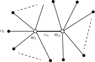
Figure 5. $\overline{\mathcal{S}}$.

A Kuranishi neighborhood of $\mathfrak{u}$ in $\mathcal{M}^{\rm RGW}_{k_{1}+1}(L;\beta_{1})\,\hat{\times}_{L}\,\mathcal{M}^{\rm RGW}_{k_{2}+1}(L;\beta_{2})$ gives a Kuranishi neighborhood of $\mathfrak{u}$ in a normalized boundary of $\mathcal{M}^{\rm RGW}_{k+1}(L;\beta)$. It contains inconsistent solutions $\mathfrak{y}=(\vec{\mathfrak{x}},\vec{\sigma},(u^{\prime}_{v}),(U^{\prime}_{v}),(\rho_{e}),(\rho_{i}))$ with respect to $\Xi$ such that $\sigma_{e_{0}}=0$. Here $e_{0}$ is the unique interior edge of level 0 of $\overline{\mathcal{S}}$. We may regard $e_{0}$ as an edge of ${\mathcal{S}}$ and $\check{R}$, too. We denote this set by $\partial_{e_{0}}\mathcal{U}(\mathfrak{u};\Upsilon)$, where $\Upsilon=(\Xi,\{E_{\mathfrak{u},\Xi}\})$.

The TSD $\Xi$ induces the TSD $\Xi_{j}$ on $\mathfrak{u}_{\mathfrak{w}_{j}}$ for $j=1,2$. We define $\Upsilon_{j}=(\Xi_{j},\{E_{\mathfrak{u}_{\mathfrak{w}_{j}},\Xi_{j}}\})$, which is a TSO. Then we obtain a Kuranishi neighborhood $\mathcal{U}(\mathfrak{u}_{\mathfrak{w}_{j}};\Upsilon_{j})$ of $\mathfrak{u}_{\mathfrak{w}_{j}}$ in the moduli space $\mathcal{M}^{\rm RGW}_{k_{j}+1}(L;\beta_{j})$, for $j=1,2$. We can define evaluation maps ${\rm ev}_{j,i}:\mathcal{U}(\mathfrak{u}_{\mathfrak{w}_{j}};\Upsilon_{j})\to L$ for $i=0,\dots,k_{j}$ and define

(3.10) $$\mathcal{U}(\mathfrak{u}_{\mathfrak{w}_{1}};\Upsilon_{1})\,{}_{{\rm ev}_{1,i}}\times_{{\rm ev}_{2,0}}\,\mathcal{U}(\mathfrak{u}_{\mathfrak{w}_{2}};\Upsilon_{2}).$$

Here $i$ is determined so that the edge $e_{0}$ is the $i$-th edge of $\mathfrak{w}_{1}$. (3.10) is a Kuranishi neighborhood of $(\mathfrak{u}_{\mathfrak{w}_{1}},\mathfrak{u}_{\mathfrak{w}_{2}})$ in the fiber product Kuranishi structure of $\mathcal{M}^{\rm RGW}_{k_{1}+1}(L;\beta_{1})\,\times_{L}\,\mathcal{M}^{\rm RGW}_{k_{2}+1}(L;\beta_{2})$.

We next define a map

$$F_{\mathfrak{u}}:\partial_{e_{0}}\mathcal{U}(\mathfrak{u};\Upsilon)\to\mathcal{U}(\mathfrak{u}_{\mathfrak{w}_{1}};\Upsilon_{1})\,{}_{{\rm ev}_{1,i}}\times_{{\rm ev}_{2,0}}\,\mathcal{U}(\mathfrak{u}_{\mathfrak{w}_{2}};\Upsilon_{2}).$$

For $j=1,2$, let $\check{R}(\mathfrak{w}_{j})$ be the very detailed DD-ribbon tree associated to $\mathfrak{w}_{j}$, defined in the beginning of this subsection. Given an inconsistent solution $\mathfrak{y}\in\partial_{e_{0}}\mathcal{U}(\mathfrak{u};\Upsilon)$, we can define $\mathfrak{y}_{(j)}=(\vec{\mathfrak{x}}_{(j)},\vec{\sigma}_{(j)},(u^{\prime}_{(j),v}),(U^{\prime}_{(j),v}),(\rho_{(j),e}),(\rho_{(j),i}))$, an inconsistent solution with respect to $\Upsilon_{j}$, as in (3.6). Identity (3.7) implies that $\mathfrak{y}_{(j)}$ satisfies [part2:kura, (8.33), (8.34)], the thickened non-linear Cauchy-Riemann equations. Thus $\mathfrak{y}_{(j)}$ is an inconsistent solution with respect to $\Upsilon_{j}$ for $j=1,2$. Since $\mathfrak{y}$ is an inconsistent solution with $\sigma_{e_{0}}=0$, we also have (see [part2:kura, Definition 8.28 (10)])

$${\rm ev}_{1,i}(\mathfrak{y}_{(1)})={\rm ev}_{2,0}(\mathfrak{y}_{(2)}).$$

Let $F_{\mathfrak{u}}(\mathfrak{y})=(\mathfrak{y}_{(1)},\mathfrak{y}_{(2)})$. We have

(3.11) $${\rm Aut}(\mathfrak{u})\subseteq{\rm Aut}(\mathfrak{u}_{\mathfrak{w}_{1}})\times{\rm Aut}(\mathfrak{u}_{\mathfrak{w}_{2}}).$$

because the restriction of all automorphisms to disk components are identity maps. Thus any $\gamma\in{\rm Aut}(\mathfrak{u})$ maps the sources curves of $\mathfrak{u}_{\mathfrak{w}_{1}}$ and $\mathfrak{u}_{\mathfrak{w}_{2}}$ to themselves. Consequently, $\gamma$ induces $(\gamma_{1},\gamma_{2})\in{\rm Aut}(\mathfrak{u}_{\mathfrak{w}_{1}})\times{\rm Aut}(\mathfrak{u}_{\mathfrak{w}_{2}})$ which determines $\gamma$ uniquely. It is then easy to see that $F_{\mathfrak{u}}$ is ${\rm Aut}(\mathfrak{u})$-invariant.

By (3.7) we have

$$\mathcal{E}_{0,\mathfrak{u},\Xi}(\mathfrak{y})\cong\bigoplus_{j=1,2}\mathcal{E}_{0,\mathfrak{u}_{\mathfrak{w}_{j}},\Xi_{j}}(\mathfrak{y}_{(j)})$$

We also have

$$\bigoplus_{e\in C^{\rm int}_{\rm th}(\check{R}),\lambda(e)>0}\mathscr{L}_{e}\cong\bigoplus_{j=1,2}\bigoplus_{e\in C^{\rm int}_{\rm th}(\check{R}(\mathfrak{w}_{j})),\lambda(e)>0}\mathscr{L}_{e}.$$

This is because the set of the edges of positive level of $\check{R}$ is the union of the set of the edges of positive level of $\check{R}(\mathfrak{w}_{1})$ and $\check{R}(\mathfrak{w}_{2})$. Therefore, we obtain a bundle map

$$\tilde{F}_{\mathfrak{u}}:\mathcal{E}_{\mathfrak{u},\Xi}\to\mathcal{E}_{\mathfrak{u}_{\mathfrak{w}_{1}},\Xi_{1}}\oplus\mathcal{E}_{\mathfrak{u}_{\mathfrak{w}_{2}},\Xi_{2}},$$

which is a lift of $F_{\mathfrak{u}}$. The bundle map $\tilde{F}_{\mathfrak{u}}$ is an isomorphism on each fiber. Therefore, we proved (a), (b) and (c) of Theorem 3.1 (2). Item (d), compatibility with Kuranishi maps, and (e), compatibility with the parametrization maps, are obvious from the construction. Item (3), compatibility with the coordinate change, is also an immediate consequence of the definitions.

It remains to prove that $F_{\mathfrak{u}}$ is an isomorphism outside the strata of codimension 2. For this purpose, it suffices to consider the cases where $\check{R}(\mathfrak{w}_{1})$ and $\check{R}(\mathfrak{w}_{2})$ have no vertex of positive level. Note that if we ignore the parameter $\rho_{i}$, then the map $F_{\mathfrak{u}}$ is a bijection. In the present case where there is no vertex of positive level, there is no parameter $\rho_{i}$. This completes the proof of Lemma 3.2. ∎

3.3. Existence of disk-component-wise Obstruction Bundle Data

The main goal of this subsection is to prove:

Proposition .

There is a system of obstruction bundle data which is disk-component-wise.

The proof is divided into 5 parts. In the first three parts, we define various objects (OBI)-(OBIII) and formulate certain conditions we require them to satisfy. In Part 4, we show that one can use these objects to obtain a system of obstruction bundle data which is disk-component-wise. Finally, in Part 5, we show the existence of objects satisfying the required conditions.

Disk-component-wise Obstruction Bundle Data: Part 1

Suppose $E$ is a positive real number and $N$ is a positive integer. Let $\mathscr{TP}$ be the set of all pairs $(k,\beta)$ such that $\mathcal{M}_{k+1}^{\rm RGW}(L;\beta)\neq\emptyset$, $\omega\cap\beta\leq E$ and $k\leq N$. Let $(k,\beta),(k^{\prime},\beta^{\prime})\in\mathscr{TP}$ we say $(k^{\prime},\beta^{\prime})<(k,\beta)$ if $\beta^{\prime}\cap\omega<\beta\cap\omega$ or $\beta^{\prime}\cap\omega=\beta\cap\omega$, $k^{\prime}<k$. We also say $(k^{\prime},\beta^{\prime})\leq(k,\beta)$ if $(k^{\prime},\beta^{\prime})<(k,\beta)$ or $(k^{\prime},\beta^{\prime})=(k,\beta)$. By Gromov compactness theorem, for each $(k,\beta)\in\mathscr{TP}$ the set $\{(k^{\prime},\beta^{\prime})\in\mathscr{TP}\mid(k^{\prime},\beta^{\prime})<(k,\beta)\}$ is a finite set.

(OBI): For $(k,\beta)\in\mathscr{TP}$, $\mathfrak{P}(k+1,\beta)$ is a finite subset of ${\rm Int}(\mathcal{M}_{k+1}^{\rm RGW}(L;\beta))$, the interior of the moduli space $\mathcal{M}_{k+1}^{\rm RGW}(L;\beta)$. To be more specific, the space ${\rm Int}(\mathcal{M}_{k+1}^{\rm RGW}(L;\beta))$ consists of elements that their source curves have only one disc component.

Let $\mathfrak{p}\in\mathfrak{P}(k+1,\beta)$. We write $\Sigma_{\mathfrak{p}}$ for the source curve of $\mathfrak{p}$ and $u_{\mathfrak{p}}:(\Sigma_{\mathfrak{p}},\partial\Sigma_{\mathfrak{p}})\to(X,L)$ for the map part of $\mathfrak{p}$. Let $\check{R}_{\mathfrak{p}}$ be the very detailed tree describing the combinatorial type of $\mathfrak{p}$. For $v\in C^{\rm int}_{0}(\check{R}_{\mathfrak{p}})$, we denote the corresponding component of $\Sigma_{\mathfrak{p}}$ by $\Sigma_{\mathfrak{p}_{v}}$ and the restriction of $\mathfrak{p}$ to $\Sigma_{\mathfrak{p}_{v}}$ by $\mathfrak{p}_{v}$.

(OBII): For any $v\in C^{\rm int}_{0}(\check{R}_{\mathfrak{p}})$, we take a finite dimensional subspace

$$E_{\mathfrak{p}_{v}}\subseteq\begin{cases}C^{\infty}(\Sigma_{\mathfrak{p}_{v}};u^{*}_{\mathfrak{p}_{v}}TX\otimes\Lambda^{0,1})&\text{if $c(v)={\rm d}$ or ${\rm s}$},\\ C^{\infty}(\Sigma_{\mathfrak{p}_{v}};u_{\mathfrak{p}_{v}}^{*}T\mathcal{D}\otimes\Lambda^{0,1})&\text{if $c(v)={\rm D}$},\end{cases}$$

whose support is away from nodal and marked points and the boundary of $\Sigma_{\mathfrak{p}_{v}}$.

We require:

Condition .

The restriction of $u_{\mathfrak{p}}$ to a neighborhood of the support of ${\rm Supp}(E_{\mathfrak{p}_{v}})$ is a smooth embedding. In particular, if ${\rm Supp}(E_{\mathfrak{p}_{v}})$ is nonzero, $u_{{\mathfrak{p}}_{v}}$ is non-constant.

Disk-component-wise Obstruction Bundle Data: Part 2

Fix $\mathfrak{u}=(\Sigma_{\mathfrak{u},v},z_{\mathfrak{u},v},u_{\mathfrak{u},v};v\in C_{0}^{\rm int}(\check{R}_{\mathfrak{u}}))\in\mathcal{M}^{\rm RGW}_{k+1}(L;\beta)$, where $\check{R}_{\mathfrak{u}}$ is the very detailed tree assigned to $\mathfrak{u}$.

There is a forgetful map from the moduli space $\mathcal{M}^{\rm RGW}_{k+1}(L;\beta)$ to the moduli space of stable discs $\mathcal{M}_{k+1}^{\rm d}$, where for any $\mathfrak{u}\in\mathcal{M}^{\rm RGW}_{k+1}(L;\beta)$ we firstly forget all the data of $\mathfrak{u}$ except the source curve $\Sigma_{\mathfrak{u}}$, and then shrink the unstable components. There is a metric space $\mathcal{C}_{k+1}^{\rm d}$, called the universal family, with a map $\pi:\mathcal{C}_{k+1}^{\rm d}\to\mathcal{M}_{k+1}^{\rm d}$ such that $\pi^{-1}(\zeta)$, for $\zeta\in\mathcal{M}_{k+1}^{\rm d}$, is a representative for $\zeta$. (See, for example, [fooo:const1, Section 2] or [part1:top, Subsection 4.1].) We pull-back $\mathcal{C}_{k+1}(L;\beta)$ to $\mathcal{M}^{\rm RGW}_{k+1}(L;\beta)$ via the forgetful map to obtain the space $\mathcal{C}^{\rm RGW}_{k+1}(L;\beta)$ with the projection map $\pi_{\rm RGW}:\mathcal{C}^{\rm RGW}_{k+1}(L;\beta)\to\mathcal{M}^{\rm RGW}_{k+1}(L;\beta)$. The pull-back of the metric on $\mathcal{C}_{k+1}(L;\beta)$ to $\mathcal{C}^{\rm RGW}_{k+1}(L;\beta)$ defines a quasi metric on $\mathcal{C}^{\rm RGW}_{k+1}(L;\beta)$. Here we obtain a quasi-metric because the forgetful map from $\mathcal{M}^{\rm RGW}_{k+1}(L;\beta)$ to $\mathcal{M}_{k+1}^{\rm d}$ is not injective. Note that this quasi metric is in fact a metric in each fiber $\pi_{\rm RGW}^{-1}(\mathfrak{u})$. The fiber $\pi_{\rm RGW}^{-1}(\mathfrak{u})$ can be identified with a quotient of $\Sigma_{\mathfrak{u}}$. Thus by pulling back the metric on each fiber $\pi_{\rm RGW}^{-1}(\mathfrak{u})$, we define a quasi metric on the source curve $\Sigma_{\mathfrak{u}}$ of $\mathfrak{u}$.

Lemma .

For each $\beta$ and $k$, there is a positive constant $\delta(k,\beta)$ with the following property. If $\mathfrak{u}\in\mathcal{M}^{\rm RGW}_{k+1}(L;\beta)$ and $v\in C^{\rm int}_{0}(\check{R}_{\mathfrak{u}})$ is a vertex with $u_{\mathfrak{u},v}:\Sigma_{\mathfrak{u},v}\to X$ being a non-constant map, then there is $x\in\Sigma_{\mathfrak{u},v}$ such that the distance between $x$ and any nodal point and boundary point of $\Sigma_{\mathfrak{u}}$ is greater than $\delta(k,\beta)$. Moreover, if $x^{\prime}\in\Sigma_{\mathfrak{u}}$ is chosen such that $u_{\mathfrak{u}}(x)=u_{\mathfrak{u}}(x^{\prime})$, then the distance between $x$ and $x^{\prime}$ is greater than $\delta(k,\beta)$.

Proof.

Given any $\mathfrak{u}$, there is a constant $\delta(k,\beta,\mathfrak{u})$ such that the lemma holds for any non-constant irreducible component $u_{\mathfrak{u},v}$ of $u_{\mathfrak{u}}$. In fact, there is a neighborhood $\mathcal{U}(\mathfrak{u})$ such that the lemma holds for the constant $\delta(k,\beta,\mathfrak{u})$ and any $\mathfrak{u}^{\prime}\in\mathcal{U}(\mathfrak{u})$. Now we can conclude the lemma using compactness of $\mathcal{M}^{\rm RGW}_{k+1}(L;\beta)$. ∎

In the following definition, $\varepsilon(k^{\prime},\beta^{\prime})$ is a constant which shall be fixed later.

Definition .

A triple $(\mathfrak{u},\mathfrak{p},\phi)$ is said to be a local approximation to ${\mathfrak{u}}$, if we have:

1. There is $(k^{\prime},\beta^{\prime})\leq(k,\beta)$ such that $\mathfrak{p}\in\mathfrak{P}(k^{\prime}+1,\beta^{\prime})$.

2. $\phi$ is a smooth embedding from a neighborhood of $\bigcup_{v}{\rm Supp}(E_{\mathfrak{p}_{v}})$ to $\Sigma_{\mathfrak{u}}$. If $x$ belongs to the image of $\phi$, then its distance to the nodal points in $\Sigma_{\mathfrak{u}}$ is greater than $\delta(k^{\prime},\beta^{\prime})$. For each $v\in C_{0}^{\rm int}(\check{R}_{\mathfrak{p}})$, there is $v^{\prime}\in C_{0}^{\rm int}(\check{R}_{\mathfrak{u}})$ such that $\phi$ maps ${\rm Supp}(E_{\mathfrak{p}_{v}})$ to $\Sigma_{\mathfrak{u},v^{\prime}}$. Furthermore, if $x^{\prime}$ is another point in the source curve of $\mathfrak{u}$ such that $u_{\mathfrak{u}}(x)=u_{\mathfrak{u}}(x^{\prime})$, then the distance between $x$ and $x^{\prime}$ is greater than $\delta(k^{\prime},\beta^{\prime})$.

3. For each $v$, we require:

   $$d_{C^{2};{\rm Supp}(E_{\mathfrak{p}_{v}})}(u_{\mathfrak{u}}\circ\phi,u_{\mathfrak{p}})<\varepsilon(k^{\prime},\beta^{\prime}).$$

4. $\phi$ satisfies the following point-wise inequality:

   $$|\overline{\partial}\phi|<|\partial\phi|/100.$$

The next definition is similar to [part2:kura, Definition 4.8]. (See also the discussion right after [part2:kura, Definition 8.17].)

Definition .

Let $(\mathfrak{u},\mathfrak{p},\phi)$ be a local approximation to ${\mathfrak{u}}$. We say a map $\hat{\phi}$ from a neighborhood of $\bigcup_{v}{\rm Supp}(E_{\mathfrak{p}_{v}})$ to $\Sigma_{\mathfrak{u}}$ is a normalization of $\phi$ if the following holds.

1. If $x$ belongs to the image of $\hat{\phi}$, then its distance to the nodal points in $\Sigma_{\mathfrak{u}}$ is greater than $\frac{1}{3}\delta(k^{\prime},\beta^{\prime})$. Furthermore, if $x^{\prime}$ is another point in the source curve of $\mathfrak{u}$ such that $u_{\mathfrak{u}}(x)=u_{\mathfrak{u}}(x^{\prime})$, then the distance between $x$ and $x^{\prime}$ is greater than $\frac{1}{3}\delta(k^{\prime},\beta^{\prime})$.

2. For each $v$, we require

   $$d_{C^{2};{\rm Supp}(E_{\mathfrak{p}_{v}})}(u_{\mathfrak{u}}\circ\hat{\phi},u_{\mathfrak{p}})<2\varepsilon(k^{\prime},\beta^{\prime}),$$

   and

   $$d_{C^{0};{\rm Supp}(E_{\mathfrak{p}_{v}})}(\hat{\phi},\phi)<\frac{\delta(k^{\prime},\beta^{\prime})}{3}.$$

3. Let $z$ be in the neighborhood of ${\rm Supp}(E_{\mathfrak{p}_{v}})$.

   1. Suppose $z$ is in a component with color ${\rm d}$ or ${\rm s}$. We take the unique minimal geodesic $\gamma$ in $X\setminus\mathcal{D}$ (with respect to the metric $g$), which joins $u_{\mathfrak{p}}(z)$ to $(u_{\mathfrak{u}}\circ\hat{\phi})(z)$. Then

      $$\frac{d\gamma}{dt}(0)\perp T_{u_{\mathfrak{p}}(z)}u_{\mathfrak{p}}(\Sigma_{\mathfrak{p}}).$$

   2. Suppose $z$ and $\hat{\phi}(z)$ are in a component with color ${\rm D}$. We take the unique minimal geodesic $\gamma$ in $\mathcal{D}$ (with respect to the metric $g^{\prime}$), which joins $u_{\mathfrak{p}}(z)$ to $(u_{\mathfrak{u}}\circ\hat{\phi})(z)$. Then

      $$\frac{d\gamma}{dt}(0)\perp T_{u_{\mathfrak{p}}(z)}u_{\mathfrak{p}}(\Sigma_{\mathfrak{p}}).$$

   3. Suppose $z$ is in a component with color ${\rm D}$ and $\hat{\phi}(z)$ is in a component with color ${\rm d}$ or ${\rm s}$. We take the unique minimal geodesic $\gamma$ in $\mathcal{D}$ (with respect to the metric $g^{\prime}$), which joins $u_{\mathfrak{p}}(z)$ to $(\pi\circ u_{\mathfrak{u}}\circ\hat{\phi})(z)$. Then

      $$\frac{d\gamma}{dt}(0)\perp T_{u_{\mathfrak{p}}(z)}u_{\mathfrak{p}}(\Sigma_{\mathfrak{p}}).$$

Lemma .

If the constant $\varepsilon(k^{\prime},\beta^{\prime})$ is small enough, then for any local approximation $(\mathfrak{u},\mathfrak{p},\phi)$ to ${\mathfrak{u}}\in\mathcal{M}^{\rm RGW}_{k+1}(L;\beta)$, there exists a normalization $\hat{\phi}$ of $\phi$ and for any other normalization $\hat{\psi}$ of $\phi$, we have:

$$\hat{\phi}|_{\bigcup_{v}{\rm Supp}(E_{\mathfrak{p}_{v}})}=\hat{\psi}|_{\bigcup_{v}{\rm Supp}(E_{\mathfrak{p}_{v}})}.$$

From now on, we assume that the constant $\varepsilon(k^{\prime},\beta^{\prime})$ satisfies the assumption of this lemma.

Proof.

This follows from the implicit function theorem and compactness of $\mathcal{M}^{\rm RGW}_{k+1}(L;\beta)$. ∎

Definition .

For $j=1,2$, suppose $(\mathfrak{u},\mathfrak{p}_{j},\phi_{j})$ is a local approximation to $\mathfrak{u}$. We say these two approximations are equivalent if $\mathfrak{p}_{1}=\mathfrak{p}_{2}$ and

$$\hat{\phi}_{1}|_{\bigcup_{v}{\rm Supp}(E_{\mathfrak{p}_{v}})}=\hat{\phi}_{2}|_{\bigcup_{v}{\rm Supp}(E_{\mathfrak{p}_{v}})}.$$

This is obviously an equivalence relation. Each equivalence class is called a quasi component (of $\mathfrak{u}$). See Figure 6 for the schematic picture of a quasi-component.

Figure 6. $[\mathfrak{u},\mathfrak{p},\phi]$ is a quasi-component of $\mathfrak{u}$

We next define obstruction spaces $E_{\mathfrak{u},{\bf p},\Xi}(\mathfrak{y})$ where ${\bf p}$ is a quasi component of $\mathfrak{u}$ and ${\mathfrak{y}}=(\vec{\mathfrak{x}},\vec{\sigma},(u^{\prime}_{v}),(U^{\prime}_{v}),(\rho_{e}),(\rho_{i}))$ is an inconsistent map with respect to a TSD $\Xi$ at $\mathfrak{u}$. The definition is similar to the corresponding definitions in [part2:kura, Subsection 9.2]. The TSD $\Xi$ induces a holomorphic embedding

$$\psi_{\mathfrak{y},\mathfrak{u}}:\bigcup_{v\in C^{\rm int}_{0}(\check{R}_{\mathfrak{u}})}\Sigma_{\mathfrak{u},v}^{-}\to\Sigma(\vec{\mathfrak{x}},\vec{\sigma}).$$

By taking $\Xi$ to be small enough, we may assume the image of $\phi$ is contained in the domain of $\psi_{\mathfrak{y},\mathfrak{u}}$. Define

$$\phi_{\mathfrak{y},\mathfrak{p}}=\psi_{\mathfrak{y},\mathfrak{u}}\circ\phi.$$

Using Implicit function theorem, we can modify $\phi_{\mathfrak{y},\mathfrak{p}}$ to obtain $\hat{\phi}_{\mathfrak{y};\mathfrak{p}}$ from a neighborhood of $\bigcup_{v}{\rm Supp}(E_{\mathfrak{p}_{v}})$ to $\Sigma_{\mathfrak{y}}$ such that the analogue of Definition 3.3 is satisfied. This map is clearly independent of the representative of ${\bf p}$ and also independent of $\Xi$ if this TSD is sufficiently small.

By replacing $I^{\rm t}_{\rm d}(x)$, $I^{\rm t}_{\rm s}(x)$ and $I^{\rm t}_{\rm D}(x)$ with $\hat{\phi}_{\mathfrak{y};\mathfrak{p}}$ and using the vector spaces $E_{\mathfrak{p}_{v}}$, we obtain

(3.12) $$E_{\mathfrak{u},{\bf p},\Xi}(\mathfrak{y})\subset\bigoplus_{v\in C^{\rm int}_{0}(\check{R}_{\mathfrak{y}})}L^{2}_{m}(\Sigma_{\mathfrak{y},v};T\otimes\Lambda^{0,1})$$

in the same way as in [part2:kura, (4.11)]. Here $\check{R}_{\mathfrak{y}}$ is the very detailed tree describing the combinatorial type of $\mathfrak{y}$.

Disk-component-wise Obstruction Bundle Data: Part 3

Our obstruction bundle data $E_{\mathfrak{u},\Xi}(\mathfrak{y})$ is a direct sum of $E_{\mathfrak{u},{\bf p},\Xi}(\mathfrak{y})$ for an appropriate set of quasi components ${\bf p}$ of $\mathfrak{u}$. Our next task is to find a way to choose this set of quasi components.

Definition .

For ${\mathfrak{u}}\in\mathcal{M}_{k+1}^{\rm RGW}(L;\beta)$, we denote by $\mathscr{QC}(k,\beta)(\mathfrak{u})$ the set of all quasi components of ${\mathfrak{u}}$. Let

$$\mathscr{QC}(k,\beta):=\bigcup_{{\mathfrak{u}}\in\mathcal{M}_{k+1}(L;\beta)}\mathscr{QC}(k,\beta)(\mathfrak{u}).$$

The map

(3.13) $$\Pi:\mathscr{QC}(k,\beta)\to\mathcal{M}_{k+1}^{\rm RGW}(L;\beta)$$

is the obvious projection.

Lemma .

If the constant $\varepsilon(k^{\prime},\beta^{\prime})$ is small enough, then $\mathscr{QC}(k,\beta)(\mathfrak{u})$ is a finite set.

Proof.

By Gromov compactness, there is only a finite number of $(k^{\prime},\beta^{\prime})\leq(k,\beta)$ such that $\mathcal{M}^{\rm RGW}_{k^{\prime}+1}(L;\beta^{\prime})\neq\emptyset$. Let $(k^{\prime},\beta^{\prime})$ be such a pair and $\mathfrak{p}$ be an element of the finite set $\mathfrak{P}(k^{\prime}+1,\beta^{\prime})$. Assume $y$ is an element of the source curve of $\mathfrak{p}$. There is a neighborhood $U_{y}$ of $y$ in the source curve of $y$ such that if $\varepsilon^{\prime}(k^{\prime},\beta^{\prime})$ is small enough, then the following holds. Let $[\mathfrak{u},\mathfrak{p},\phi]$ and $[\mathfrak{u},\mathfrak{p},\psi]$ be two quasi components of an element $\mathfrak{u}\in\mathcal{M}^{\rm RGW}_{k+1}(L;\beta)$ with $\hat{\phi}$ and $\hat{\psi}$ being the normalizations of $\phi$ and $\psi$. If $\hat{\phi}(y)\neq\hat{\psi}(y)$, then $\hat{\phi}|_{U_{y}}$ and $\hat{\psi}|_{U_{y}}$ are disjoint. This would imply that given the element $\mathfrak{u}$, there are only finitely many possibilities for the restriction of the normalization map to $U_{y}$. Therefore, there are finitely many quasi components of the form $[\mathfrak{u},\mathfrak{p},\phi]$ for $\mathfrak{u}$. Finiteness of the sets $\mathfrak{P}(k^{\prime}+1,\beta^{\prime})$ completes the proof. ∎

We next define a topology on $\mathscr{QC}(k,\beta)$. Let ${\mathfrak{u}}\in\mathcal{M}_{k+1}^{\rm RGW}(L;\beta)$, $\Xi$ be a TSD at $\mathfrak{u}$ and $\mathfrak{U}({\mathfrak{u}},\Xi)$ be the associated set of inconsistent solutions. (See [part2:kura, Definition 8.28].) We construct a map

$$\mathfrak{I}:\mathfrak{U}({\mathfrak{u}},\Xi)\cap\mathcal{M}_{k+1}^{\rm RGW}(L;\beta)\to\mathscr{QC}(k,\beta).$$

such that $\Pi\circ\mathfrak{I}={\rm id}$ assuming $\Xi$ is small enough. The TSD $\Xi$ induces a map

$$\psi_{\mathfrak{u}^{\prime},\mathfrak{u}}:\bigcup_{v\in C^{\rm int}_{0}(\check{R}_{\mathfrak{u}})}\Sigma_{\mathfrak{u},v}^{-}\to\Sigma_{\mathfrak{u}^{\prime}}$$

for $\mathfrak{u}^{\prime}\in\mathfrak{U}({\mathfrak{u}},\Xi)$. Let $(\mathfrak{u},\mathfrak{p},\phi)$ be a local approximation to ${\mathfrak{u}}$. If $\Xi$ is sufficiently small, then $(\mathfrak{u},\mathfrak{p},\psi_{\mathfrak{u}^{\prime},\mathfrak{u}}\circ\phi)$ is a local approximation to ${\mathfrak{u}}^{\prime}$. Using Implicit function theorem, it is easy to see that the equivalence class of $(\mathfrak{u},\mathfrak{p},\psi_{\mathfrak{u}^{\prime},\mathfrak{u}}\circ\phi)$ depends only on the equivalence class of $(\mathfrak{u},\mathfrak{p},\phi)$. We thus obtain the map $\mathfrak{I}$. This map in a small neighborhood of $\mathfrak{u}$ is independent of the choice of $\Xi$. The map $\mathfrak{I}$ is also injective.

Definition .

A neighborhood system of a quasi component ${\bf p}=[\mathfrak{u},\mathfrak{p},\phi]$ of $\mathfrak{u}$ in $\mathscr{QC}(k,\beta)$ is given by mapping the neighborhood system of $\mathfrak{u}$ in $\mathcal{M}_{k+1}^{\rm RGW}(L;\beta)$ via the map $\mathfrak{I}$.

The following is a straightforward consequence of the definition.

Lemma .

$\mathscr{QC}(k,\beta)$ is Hausdorff and metrizable with respect to this topology. For each quasi component ${\bf p}$ of $\mathfrak{u}$, there exists a neighborhood of ${\bf p}$ in $\mathscr{QC}(k,\beta)$ such that the restriction of $\Pi$ to this neighborhood is a homeomorphism onto an open subset.

Let $\mathscr{F}$ be a subset of $\mathscr{QC}(k,\beta)$. For $\mathfrak{u}\in\mathcal{M}_{k+1}(L;\beta)$, we define

$$\mathscr{F}(\mathfrak{u})=\Pi^{-1}(\mathfrak{u})\cap\mathscr{F}.$$

It is a map which assigns to $\mathfrak{u}$ a finite set of quasi components of $\mathfrak{u}$. Justified by this, we call $\mathscr{F}$ a quasi component choice map.

Definition .

A quasi component choice map $\mathscr{F}$ is open (resp. closed) if it is an open (resp. closed) subset of $\mathscr{QC}(k,\beta)$ (with respect to the topology of Definition 3.3). We say $\mathscr{F}$ is proper if the restriction of $\Pi$ to $\mathscr{F}$ is proper.

(OBIII): For each $(k,\beta)\in\mathscr{TP}$, we take quasi component choice maps $\mathscr{F}_{k,\beta}$ and $\mathscr{F}^{\circ}_{k,\beta}$.

We are mainly concerned with the objects as in (OBIII) which satisfy the following condition.

Condition .

The quasi component choice map $\mathscr{F}^{\circ}_{k,\beta}$ is open and is a subset of $\mathscr{F}_{k,\beta}$. The quasi component map $\mathscr{F}_{k,\beta}$ is proper.

The next condition is related to the disk-component-wise-ness. Let ${\mathfrak{u}}\in\mathcal{M}_{k+1}^{\rm RGW}(L;\beta)$ and $\check{R}$ be the very detailed tree associated to $\mathfrak{u}$. Let $\check{R}$ belong to the disk splitting tree $\mathcal{S}$. Let $\mathfrak{w}$ be an interior vertex of ${\mathcal{S}}$. Following the discussion of the beginning of Subsection 3.2, we obtain an element $\mathfrak{u}_{\mathfrak{w}}\in\mathcal{M}_{k_{\mathfrak{w}}+1}^{\rm RGW}(L;\beta(\mathfrak{w}))$ for each interior vertex $\mathfrak{w}$ of $\mathcal{S}$. Define

(3.14) $$\mathscr{I}_{\mathfrak{w}}:\mathscr{QC}(k_{\mathfrak{w}},\beta(\mathfrak{w}))(\mathfrak{u}_{\mathfrak{w}})\to\mathscr{QC}(k,\beta)(\mathfrak{u})$$

to be the map given by:

$$\mathscr{I}_{\mathfrak{w}}([\mathfrak{u}_{\mathfrak{w}},\mathfrak{p},\phi])=[\mathfrak{u},\mathfrak{p},\phi].$$

The target of $\phi$ on the left hand side is $\Sigma_{\mathfrak{u}_{\mathfrak{w}}}$, the source curve of $\mathfrak{u}_{\mathfrak{w}}$, which is a subset of the source curve $\Sigma_{\mathfrak{u}}$ of $\mathfrak{u}$. So $\phi$ on the right hand side is regarded as a map to $\Sigma_{\mathfrak{u}}$. It is clear that $\mathscr{I}_{\mathfrak{w}}$ maps equivalent objects to equivalent ones and hence the above definition is well-defined.

Lemma .

The map $\mathscr{I}_{\mathfrak{w}}$ is injective. If $\mathfrak{w}\neq\mathfrak{w}^{\prime}$, then the image of $\mathscr{I}_{\mathfrak{w}}$ is disjoint from the image of $\mathscr{I}_{\mathfrak{w}^{\prime}}$.

Proof.

The injectivity is obvious from the definition. If $[\mathfrak{u},\mathfrak{p},\phi]$ is in the image of $\mathscr{I}_{\mathfrak{w}}$, then the image of $\phi$ is contained in the component $\Sigma_{\mathfrak{u},\mathfrak{w}}$ corresponding to $\mathfrak{w}$. Therefore, for $\mathfrak{w}\neq\mathfrak{w}^{\prime}$, the image of the maps $\mathscr{I}_{\mathfrak{w}}$ and $\mathscr{I}_{\mathfrak{w}^{\prime}}$ are disjoint. ∎

Condition .

Let ${\mathfrak{u}}\in\mathcal{M}_{k+1}^{\rm RGW}(L;\beta)$ and $\check{R}$ and $\mathcal{S}$ be given as above. Then we require

(3.15) $$\mathscr{F}_{k,\beta}({\mathfrak{u}}) =\bigcup_{\mathfrak{w}}\mathscr{I}_{\mathfrak{w}}\left(\mathscr{F}_{k_{\mathfrak{w}},\beta_{\mathfrak{w}}}({\mathfrak{u}}_{\mathfrak{w}})\right),$$

$$\mathscr{F}^{\circ}_{k,\beta}({\mathfrak{u}}) =\bigcup_{\mathfrak{w}}\mathscr{I}_{\mathfrak{w}}\left(\mathscr{F}^{\circ}_{k_{\mathfrak{w}},\beta_{\mathfrak{w}}}({\mathfrak{u}}_{\mathfrak{w}})\right).$$

We need the following definition to state the next condition:

Definition .

Let ${\mathfrak{u}}\in\mathcal{M}_{k+1}^{\rm RGW}(L;\beta)$ and $\mathfrak{y}$ be an inconsistent map with respect to a TSD $\Xi$ at $\mathfrak{u}$. We assume $\Xi$ is sufficiently small such that the vector spaces $E_{\mathfrak{u},{\bf p},\Xi}(\mathfrak{y})$ in (3.12) are well-defined. We define

(3.16) $$E_{\mathfrak{u},\mathscr{F},\Xi}(\mathfrak{y}):= \sum_{[\bf p]\in\mathscr{F}_{k,\beta}({\mathfrak{u}})}E_{\mathfrak{u},{\bf p},\Xi}(\mathfrak{y})\subset\bigoplus_{v\in C^{\rm int}_{0}(\check{R})}L^{2}_{m}(\Sigma_{\mathfrak{y},v};T\otimes\Lambda^{0,1}),$$

where $\Sigma$ denotes the sum of vector subspaces of a vector space. Similarly, we define

(3.17) $$E_{\mathfrak{u},\mathscr{F}^{\circ},\Xi}(\mathfrak{y}):= \sum_{[\bf p]\in\mathscr{F}^{\circ}_{k,\beta}({\mathfrak{u}})}E_{\mathfrak{u},{\bf p},\Xi}(\mathfrak{y})\subset\bigoplus_{v\in C^{\rm int}_{0}(\check{R})}L^{2}_{m}(\Sigma_{\mathfrak{y},v};T\otimes\Lambda^{0,1}).$$

Note that $E_{\mathfrak{u},\mathscr{F}^{\circ},\Xi}(\mathfrak{y})\subseteq E_{\mathfrak{u},\mathscr{F},\Xi}(\mathfrak{y})$.

Condition .

We require that the sum in (3.16) is a direct sum for $\mathfrak{y}=\mathfrak{u}$. Namely,

(3.18) $$E_{\mathfrak{u},\mathscr{F},\Xi}(\mathfrak{u})= \bigoplus_{[\bf p]\in\mathscr{F}_{k,\beta}({\mathfrak{u}})}E_{\mathfrak{u},{\bf p},\Xi}(\mathfrak{y}).$$

Note that the above condition implies that the sum in (3.17) for $\mathfrak{y}=\mathfrak{u}$ is also a direct sum.

Definition .

We say the linearization of the non-linear Cauchy-Riemann equation is transversal to $E_{\mathfrak{u},\mathscr{F}^{\circ},\Xi}(\mathfrak{u})$ if the sum of the images of the operator $D_{\mathfrak{u}}\overline{\partial}$ in [part2:kura, (8.3)] and $E_{\mathfrak{u},\mathscr{F}^{\circ},\Xi}(\mathfrak{u})$ is $L^{2}_{m,\delta}(\mathfrak{u};T\otimes\Lambda^{0,1})$.

Definition .

Consider the operator:

$$\mathcal{EV}_{z_{0}}:W^{2}_{m+1,\delta}(\mathfrak{u};T)\to T_{u(z_{0})}L$$

given by evaluation at the point $z_{0}$, the 0-th boundary marked point of the source of $\mathfrak{u}$. Recall that the Hilbert space $W^{2}_{m+1,\delta}(\mathfrak{u};T)$ is the domain of the operator $D_{\mathfrak{u}}\overline{\partial}$ in [part2:kura, (8.3)]. We say $E_{\mathfrak{u},\mathscr{F}^{\circ},\Xi}(\mathfrak{u})$ satisfies the mapping transversality property, if the restriction

$$\mathcal{EV}_{z_{0}}|_{D_{\mathfrak{u}}\overline{\partial}^{-1}(E_{\mathfrak{u},\mathscr{F}^{\circ},\Xi}(\mathfrak{u}))}:D_{\mathfrak{u}}\overline{\partial}^{-1}(E_{\mathfrak{u},\mathscr{F}^{\circ},\Xi}(\mathfrak{u}))\to T_{u(z_{0})}L,$$

is surjective.

Condition .

We require that the linearization of the non-linear Cauchy-Riemann equation is transversal to $E_{\mathfrak{u},\mathscr{F}^{\circ},\Xi}(\mathfrak{u})$ and $E_{\mathfrak{u},\mathscr{F}^{\circ},\Xi}(\mathfrak{u})$ satisfies the mapping transversality property.

Let ${\rm Aut}(\mathfrak{u})$ be the group of automorphisms of $\mathfrak{u}$. If $\gamma\in{\rm Aut}(\mathfrak{u})$ and $[\mathfrak{u},\mathfrak{p},\phi]$ is a quasi component of $\mathfrak{u}$, then $[\mathfrak{u},\mathfrak{p},\gamma\circ\phi]$ is also a quasi component of $\mathfrak{u}$. Thus ${\rm Aut}(\mathfrak{u})$ acts on $\mathscr{QC}(k,\beta)(\mathfrak{u})$.

Condition .

We require that $\mathscr{F}_{k,\beta}({\mathfrak{u}})$, $\mathscr{F}^{\circ}_{k,\beta}({\mathfrak{u}})$ are invariant with respect to the action of ${\rm Aut}(\mathfrak{u})$.

Disk-component-wise Obstruction Bundle Data: Part 4

Given the above objects satisfying the mentioned conditions, we can construct the desired obstruction bundle data:

Lemma .

Suppose we are given the objects in (OBI)-(OBIII), which satisfy Conditions 3.3, 3.3, 3.3, 3.3, 3.3. Then $\{E_{\mathfrak{u},\mathscr{F},\Xi}(\mathfrak{y})\}$ is a disk-component-wise system of obstruction bundle data.

Proof.

The system $\{E_{\mathfrak{u},\mathscr{F},\Xi}(\mathfrak{y})\}$ satisfies Definition 3.2 (1), (2), (3) and (5) as immediate consequences of the construction. Definition 3.2 (3) is a consequence of the properness of $\mathscr{F}_{k,\beta}$. (Compare to [part2:kura, Lemma 9.39].) Definition 3.2 (5) is a consequence of Condition 3.3. Definition 3.2 (6) is a consequence of Condition 3.3. Disc-component-wise-ness is an immediate consequence of Condition 3.3. ∎

Disk-component-wise Obstruction Bundle Data: Part 5

To complete the proof of Proposition 3.3, it suffices to prove the next lemma.

Lemma .

There exist objects (OBI)-(OBIII) which satisfy Conditions 3.3, 3.3, 3.3, 3.3 and 3.3.

Proof.

The proof is by induction on $(k,\beta)$ and is given in several steps. Here we denote $(k,\beta)<(k^{\prime},\beta^{\prime})$ when either $\beta\cap[\omega]<\beta^{\prime}\cap[\omega]$ or $\beta\cap[\omega]=\beta^{\prime}\cap[\omega]$, $k<k^{\prime}$.

Step 1 (The base of induction): We assume that $(k,\beta)$ is minimal in this order $<$. In this case, the moduli space $\mathcal{M}_{k+1}^{\rm RGW}(L;\beta)$ has no boundary. We follow a similar argument as in [part2:kura, Subsection 9.2]. For each $\mathfrak{p}\in\mathcal{M}_{k+1}^{\rm RGW}(L;\beta)$, we fix a vector space $E_{\mathfrak{p},v}$ for $v\in C^{0}_{\rm int}(\check{R}_{\mathfrak{p}})$ as in (OBII). We require that the linearization of the non-linear Cauchy-Riemann equation is transversal to

(3.19) $$\bigoplus_{v\in C^{0}_{\rm int}(\check{R}_{\mathfrak{p}})}E_{\mathfrak{p},v}$$

at $\mathfrak{p}$ (Definition 3.3) and (3.19) has the mapping transversality property at $\mathfrak{p}$ (Definition 3.3). Using Lemma 3.3, we may assume that the distance of any point $x$ in the support of the elements of $E_{\mathfrak{p},v}$ to nodal points of $\Sigma_{\mathfrak{p}}$ is at least $\delta(k,\beta)$. Moreover, if $x^{\prime}$ is another point in the source curve of $\mathfrak{p}$ such that $u_{\mathfrak{p}}(x)=u_{\mathfrak{p}}(x^{\prime})$, then the distance between $x$ and $x^{\prime}$ is greater than $\delta(k^{\prime},\beta^{\prime})$.

For each $\mathfrak{p}$, we also pick a TSD $\Xi_{\mathfrak{p}}$ and a compact neighborhood $\mathcal{K}(\mathfrak{p})$ of $\mathfrak{p}$ in $\mathcal{M}_{k+1}^{\rm RGW}(L;\beta)$, which satisfy the following conditions. Firstly we require that the compact neighborhood $\mathcal{K}(\mathfrak{p})$ is included in the set of inconsistent maps determined by $\Xi_{\mathfrak{p}}$. Thus for any $\mathfrak{u}\in\mathcal{K}(\mathfrak{p})$, there is a holomorphic embedding $\phi_{\mathfrak{u},\mathfrak{p}}$ from a neighborhood of $\bigcup_{v}{\rm Supp}(E_{\mathfrak{p}_{v}})$ to $\Sigma_{\mathfrak{u}}$, assuming that $\Xi_{\mathfrak{p}}$ is small enough. We may also assume that we can normalize $\phi_{\mathfrak{u},\mathfrak{p}}$ as in Definition 3.3 to obtain:

$$\hat{\phi}_{\mathfrak{u},\mathfrak{p}}:\bigcup_{v}{\rm Supp}(E_{\mathfrak{p}_{v}})\to\Sigma_{\mathfrak{u}}.$$

We use $\hat{\phi}_{\mathfrak{u},\mathfrak{p}}$ to transport $E_{\mathfrak{p},v}$ to the point $\mathfrak{u}$ and obtain $E_{\mathfrak{p},v}(\mathfrak{u})$. We may choose $\Xi_{\mathfrak{p}}$ small enough such that the linearization of the non-linear Cauchy-Riemann equation is transversal to

(3.20) $$E_{\mathfrak{p},v}(\mathfrak{u})=\bigoplus_{v\in C^{0}_{\rm int}(\check{R}_{\mathfrak{p}})}E_{\mathfrak{p},v}(\mathfrak{u})$$

at $\mathfrak{u}$ and (3.20) satisfies the mapping transversality property at $\mathfrak{u}$, for any $\mathfrak{u}\in\mathcal{K}(\mathfrak{p})$.

Now we take a finite set $\mathfrak{P}(k+1,\beta)\subset\mathcal{M}_{k+1}^{\rm RGW}(L;\beta)$ such that

(3.21) $$\bigcup_{\mathfrak{p}\in\mathfrak{P}(k+1,\beta)}{\rm Int}\,\mathcal{K}(\mathfrak{p})=\mathcal{M}_{k+1}^{\rm RGW}(L;\beta).$$

We define

(3.22) $$\mathscr{F}_{k,\beta}(\mathfrak{u}) =\{[\mathfrak{u},\mathfrak{p},\phi_{\mathfrak{u},\mathfrak{p}}]\mid\mathfrak{p}\in\mathfrak{P}(k+1,\beta),\,\,\mathfrak{u}\in\mathcal{K}(\mathfrak{p})\},$$

$$\mathscr{F}^{\circ}_{k,\beta}(\mathfrak{u}) =\{[\mathfrak{u},\mathfrak{p},\phi_{\mathfrak{u},\mathfrak{p}}]\mid\mathfrak{p}\in\mathfrak{P}(k+1,\beta),\,\,\mathfrak{u}\in{\rm Int}\,\mathcal{(}K(\mathfrak{p}))\}.$$

Condition 3.3 is immediate from the definition. Condition 3.3 is void in this case. We can perturb $E_{\mathfrak{p},v}$ arbitrarily small in $C^{2}$ topology so that Condition 3.3 holds. (See [fooo:const2, Lemma 9.9].) Condition 3.3 follows from the choice of $E_{\mathfrak{p},v}$ and (3.21). We can take $E_{\mathfrak{p},v}$ to be invariant under the action of ${\rm Aut}(\mathfrak{p})$ and hence Condition 3.3 holds. Thus we complete the first step of the induction.

Next, we suppose that the required objects in (OBI)-(OBIII) are defined for $(k^{\prime},\beta^{\prime})$ with $(k^{\prime},\beta^{\prime})<(k,\beta)$. We use Condition 3.3 to define $\mathscr{F}^{\prime}_{k,\beta}(\mathfrak{u})$, $\mathscr{F}^{\prime\circ}_{k,\beta}(\mathfrak{u})$ for $\mathfrak{u}\in\partial\mathcal{M}_{k+1}(L;\beta)$.

Step 2:  The set:

$$\bigcup_{\mathfrak{u}\in\partial\mathcal{M}_{k+1}(L;\beta)}\mathscr{F}^{\prime\circ}_{k,\beta}(\mathfrak{u})$$

is an open subset of $\Pi^{-1}(\partial\mathcal{M}_{k+1}(L;\beta))$, where $\Pi$ is the map in (3.13).

Let ${\bf p}_{j}\in\mathscr{QC}(k,\beta)$ with $\mathfrak{u}_{j}=\Pi({\bf p}_{j})\in\partial\mathcal{M}^{\rm RGW}_{k+1}(L;\beta)$. Suppose also $\lim_{j\to\infty}{\bf p}_{j}={\bf p}\in\mathscr{F}^{\prime\circ}_{k,\beta}(\mathfrak{u})$ with $\mathfrak{u}=\lim_{j\to\infty}\mathfrak{u}_{j}$. We need to show that ${\bf p}_{j}\in\mathscr{F}^{\prime\circ}_{k,\beta}(\mathfrak{u}_{j})$ for sufficiently large values of $j$. Let the combinatorial type of $\mathfrak{u}$ be given by a very detailed DD-ribbon tree $\check{R}$ which belongs to the disc splitting tree $\mathcal{S}$. We may assume that the very detailed tree associated to $\mathfrak{u}_{j}$ is independent of $j$ because there are finitely many very detailed tree obtained by level shrinking, level $0$ edge shrinking and fine edge shrinking. We denote this very detailed DD-ribbon tree by $\check{R}^{\prime}$. We also assume that $\check{R}^{\prime}$ belongs to the disc splitting tree $\mathcal{S}^{\prime}$. Since $\mathcal{S}^{\prime}$ is obtained from $\mathcal{S}$ by shrinking level $0$ edges, there is a standard shrinking map $\pi:\mathcal{S}\to\mathcal{S}^{\prime}$. Note that $\mathcal{S}$ and $\mathcal{S}^{\prime}$ have at least two interior vertices.

By Condition 3.3, there exists $\mathfrak{w}\in C^{0}_{\rm int}(\mathcal{S})$ and ${\bf p}_{\mathfrak{w}}\in\mathscr{F}^{\circ}_{k,\beta}(\mathfrak{u}_{\mathfrak{w}})$ such that

$${\bf p}=\mathscr{I}_{\mathfrak{w}}({\bf p}_{\mathfrak{w}}).$$

Let ${\mathfrak{w}}^{\prime}=\pi(\mathfrak{w})$, which is an interior vertex of $\mathcal{S}^{\prime}$. We also define $\mathcal{S}(\mathfrak{w}^{\prime}):=\pi^{-1}(\mathfrak{w}^{\prime})$, which is a subtree of $\mathcal{S}$. Let ${\mathfrak{u}}_{\mathcal{S}(\mathfrak{w}^{\prime})}$ be an object of $\mathcal{M}^{\rm RGW}_{k_{\mathfrak{w}^{\prime}}+1}(L;\beta_{\mathfrak{w}^{\prime}})$ which is obtained from $\mathfrak{u}$ and $\mathcal{S}(\mathfrak{w}^{\prime})$ in the same way as in the beginning of Subsection 3.2. Convergence of $\mathfrak{u}_{j}$ to $\mathfrak{u}$ implies

$$\lim_{j\to\infty}\mathfrak{u}_{j,{\mathfrak{w}}^{\prime}}={\mathfrak{u}}_{\mathcal{S}(\mathfrak{w}^{\prime})}$$

by the definition of the RGW topology.

Since ${\mathfrak{w}}$ is a vertex of $\mathfrak{R}(\mathfrak{w}^{\prime})$, there exists:

$$\mathscr{I}^{\prime}_{\mathfrak{w}}:\mathscr{QC}(k_{\mathfrak{w}},\beta_{\mathfrak{w}})(\mathfrak{u}_{\mathfrak{w}})\to\mathscr{QC}(k_{\mathfrak{w}^{\prime}},\beta_{\mathfrak{w}^{\prime}})({\mathfrak{u}}_{\mathcal{S}(\mathfrak{w}^{\prime})}).$$

We define ${\bf p}_{\mathfrak{w}^{\prime}}=\mathscr{I}^{\prime}_{\mathfrak{w}}({\bf p}_{\mathfrak{w}}).$ Using the definition of the topology of $\mathscr{QC}(k,\beta)$ and of $\mathscr{I}_{\mathfrak{w}}$, it is easy to see that there exists ${\bf p}_{j,\mathfrak{w}^{\prime}}\in\mathscr{QC}(k_{\mathfrak{w}^{\prime}},\beta_{\mathfrak{w}^{\prime}})(\mathfrak{u}_{j,{\mathfrak{w}}^{\prime}})$ such that

$$\lim_{j\to\infty}{\bf p}_{j,\mathfrak{w}^{\prime}}={\bf p}_{\mathfrak{w}^{\prime}}$$

in $\mathscr{QC}(k_{\mathfrak{w}^{\prime}},\beta_{\mathfrak{w}^{\prime}})$ and

$$\mathscr{I}^{\prime}_{\mathfrak{w}}({\bf p}_{j,\mathfrak{w}^{\prime}})={\bf p}_{j}.$$

Now by induction hypothesis

$${\bf p}_{j,\mathfrak{w}^{\prime}}\in\mathscr{F}^{\circ}_{k_{\mathfrak{w}^{\prime}},\beta_{\mathfrak{w}^{\prime}}}(\mathfrak{u}_{j,{\mathfrak{w}^{\prime}}})$$

for sufficiently large $j$. Condition 3.3 implies ${\bf p}_{j}\in\mathscr{F}^{\prime\circ}_{k,\beta}(\mathfrak{u}_{j})$ for large $j$, as required.

Step 3: The restriction of $\Pi$ to

$$\bigcup_{\mathfrak{u}\in\partial\mathcal{M}_{k+1}(L;\beta)}\mathscr{F}^{\prime}_{k,\beta}(\mathfrak{u})$$

is a proper map to $\partial\mathcal{M}_{k+1}^{\rm RGW}(L;\beta)$.

Let ${\bf p}_{j}\in\mathscr{F}^{\prime}_{k,\beta}(\mathfrak{u}_{j})$ with $\mathfrak{u}_{j}\in\partial\mathcal{M}^{\rm RGW}_{k+1}(L;\beta)$. Suppose $\lim_{j\to\infty}\mathfrak{u}_{j}=\mathfrak{u}\in\partial\mathcal{M}^{\rm RGW}_{k+1}(L;\beta)$. It suffices to find a subsequence of ${\bf p}_{j}$ which converges to an element of $\mathscr{F}^{\prime}_{k,\beta}(\mathfrak{u})$. Let the combinatorial type of $\mathfrak{u}$ be given by a very detailed DD-ribbon tree $\check{R}$ which belongs to the disc splitting tree $\mathcal{S}$. After passing to a subsequence, we may assume that the very detailed tree associated to $\mathfrak{u}_{j}$ is independent of $j$. We denote this tree by $\check{R}^{\prime}$ which belongs to the disc splitting tree $\mathcal{S}^{\prime}$. Let $\pi:\mathcal{S}\to\mathcal{S}^{\prime}$ be defined as in the previous step.

By Condition 3.3 and after passing to a subsequence, we may assume that there exist $\mathfrak{w}\in C^{0}_{\rm int}(\mathcal{S}^{\prime})$ and ${\bf p}_{j,\mathfrak{w}}\in\mathscr{F}^{\prime}_{k_{\mathfrak{w}},\beta_{\mathfrak{w}}}(\mathfrak{u}_{j,\mathfrak{w}})$ such that

$$\mathscr{I}_{\mathfrak{w}}({\bf p}_{j,\mathfrak{w}})={\bf p}_{j}.$$

Let $\mathcal{S}_{\mathfrak{w}}$ be the subtree $\pi^{-1}(\mathfrak{w})$ of $\mathcal{S}$. We obtain $\mathfrak{u}_{\mathfrak{R}_{\mathfrak{w}}}$ from $\mathfrak{u}$ in the same way as in the beginning of Subsection 3.2. Convergence of $\mathfrak{u}_{j}$ to $\mathfrak{u}$ implies that

$$\lim_{j\to\infty}\mathfrak{u}_{j,\mathfrak{w}}=\mathfrak{u}_{\mathfrak{R}_{\mathfrak{w}}}$$

by the definition of the RGW topology. Now we use the induction hypothesis to find a subsequence such that ${\bf p}_{j,\mathfrak{w}}\in\mathscr{F}^{\prime}_{k_{\mathfrak{w}},\beta_{\mathfrak{w}}}(\mathfrak{u}_{j,\mathfrak{w}})$ converges to ${\bf p}_{\mathfrak{w}}\in\mathscr{F}^{\prime}_{k_{\mathfrak{w}},\beta_{\mathfrak{w}}}(\mathfrak{u}_{\mathfrak{R}_{\mathfrak{w}}}).$ Therefore

$$\lim_{j\to\infty}{\bf p}_{j}=\mathscr{I}_{\mathfrak{w}}({\bf p}_{\mathfrak{w}})\in\mathscr{F}^{\prime}_{k,\beta}(\mathfrak{u}).$$

This completes the proof of this step.

Step 4: (Extension to a neighborhood of the boundary) In the previous steps, we defined $\mathscr{F}^{\prime}_{k,\beta}$ and $\mathscr{F}^{\prime\circ}_{k,\beta}$ on the boundary. Next, we extend these quasi component choice maps to a neighborhood of the boundary. We fix $\rho>0$ sufficiently small such that if $d(\mathfrak{u},\mathfrak{u}^{\prime})<5\rho$, $\mathfrak{u}^{\prime}\in\partial\mathcal{M}_{k+1}^{\rm RGW}(L;\beta)$ and $[\mathfrak{u}^{\prime},\mathfrak{p},\phi]\in\mathscr{F}^{\prime}_{k,\beta}(\mathfrak{u}^{\prime})$, then $[\mathfrak{u},\mathfrak{p},\psi_{\mathfrak{u},\mathfrak{u}^{\prime}}\circ\phi]$ is a quasi component. Then for $\mathfrak{u}\in\mathcal{M}_{k+1}^{\rm RGW}(L;\beta)$ with $d(\mathfrak{u},\partial\mathcal{M}_{k+1}^{\rm RGW}(L;\beta))<2\rho$, we define

1. $\mathscr{F}^{\prime}_{k,\beta}(\mathfrak{u})$ is the set of $[\mathfrak{u},\mathfrak{p},\phi]$ such that there are $\mathfrak{u}^{\prime}\in\partial\mathcal{M}^{\rm RGW}_{k+1}(L;\beta)$ and $[\mathfrak{u}^{\prime},\mathfrak{p},\phi^{\prime}]\in\mathscr{F}^{\prime}_{k,\beta}(\mathfrak{u}^{\prime})$ with the following properties:

   1. $d(\mathfrak{u},\mathfrak{u}^{\prime})\leq 2d(\mathfrak{u},\partial\mathcal{M}^{\rm RGW}_{k+1}(L;\beta))\leq\rho$.

   2. $(\mathfrak{u},\mathfrak{p},\phi)$ is equivalent to $(\mathfrak{u},\mathfrak{p},\psi_{\mathfrak{u},\mathfrak{u}^{\prime}}\circ\phi^{\prime})$.

2. $\mathscr{F}^{\prime\circ}_{k,\beta}(\mathfrak{u})$ is the set of $[\mathfrak{u},\mathfrak{p},\phi]$ such that there are $\mathfrak{u}^{\prime}\in\partial\mathcal{M}^{\rm RGW}_{k+1}(L;\beta)$ and $[\mathfrak{u}^{\prime},\mathfrak{p},\phi^{\prime}]\in\mathscr{F}^{\prime\circ}_{k,\beta}(\mathfrak{u}^{\prime})$ with the following properties:

   1. $\mathfrak{u}=\mathfrak{u}^{\prime}$ or $d(\mathfrak{u},\mathfrak{u}^{\prime})<2d(\mathfrak{u},\partial\mathcal{M}^{\rm RGW}_{k+1}(L;\beta))<\rho$.

   2. $(\mathfrak{u},\mathfrak{p},\phi)$ is equivalent to $(\mathfrak{u},\mathfrak{p},\psi_{\mathfrak{u},\mathfrak{u}^{\prime}}\circ\phi^{\prime})$.

We put

$$\mathscr{F}^{\prime\circ}_{k,\beta}=\bigcup_{\mathfrak{u}}\mathscr{F}^{\prime\circ}_{k,\beta}(\mathfrak{u}),\qquad\mathscr{F}^{\prime}_{k,\beta}=\bigcup_{\mathfrak{u}}\mathscr{F}^{\prime}_{k,\beta}(\mathfrak{u}).$$

It follows easily from Step 2 that $\mathscr{F}^{\prime\circ}_{k,\beta}$ is open. It follows easily from Step 3 that the restriction of $\Pi$ to $\mathscr{F}^{\prime\circ}_{k,\beta}$ is proper.

Items (b) in the above definition implies that $\mathscr{F}^{\prime}_{k,\beta}(\mathfrak{u})$ and $\mathscr{F}^{\prime\circ}_{k,\beta}(\mathfrak{u})$ coincide with the previously defined spaces for $\mathfrak{u}\in\partial\mathcal{M}^{\rm RGW}_{k+1}(L;\beta)$. Therefore, Condition 3.3 holds. Thus we have constructed objects for $(k,\beta)$ which satisfy all the required conditions except Condition 3.3. By taking a smaller value of $\rho$ if necessary, we can guarantee that Condition 3.3 is also satisfied.

Step 5: (Extension to the rest of the moduli space $\mathcal{M}_{k+1}^{\rm RGW}(L;\beta)$) The rest of the proof is similar to Step 1. For each $\mathfrak{p}\in{\rm Int}(\mathcal{M}^{\rm RGW}_{k+1}(L;\beta))$ we choose $\Xi_{\mathfrak{p}}$ , $E_{\mathfrak{p},v}$ and $\mathcal{K}(\mathfrak{p})$ as in the first step of the induction. We take a finite set $\mathfrak{P}(k+1,\beta)$ such that

(3.23) $$\bigcup_{\mathfrak{p}\in\mathfrak{P}(k+1,\beta)}{\rm Int}\,\mathcal{K}(\mathfrak{p})=\mathcal{M}^{\rm RGW}_{k+1}(L;\beta)\setminus B_{\rho}(\partial\mathcal{M}^{\rm RGW}_{k+1}(L;\beta)).$$

is satisfied instead of (3.21). Now we define

(3.24) $$\mathscr{F}_{k,\beta}(\mathfrak{u}) =\mathscr{F}^{\prime}_{k,\beta}(\mathfrak{u})\cup\{[\mathfrak{u},\mathfrak{p},\phi_{\mathfrak{u},\mathfrak{p}}]\mid\mathfrak{p}\in\mathfrak{P}(k,\beta),\,\,\mathfrak{u}\in\mathcal{K}(\mathfrak{p})\}$$

$$\mathscr{F}^{\circ}_{k,\beta}(\mathfrak{u}) =\mathscr{F}^{\prime\circ}_{k,\beta}(\mathfrak{u})\cup\{[\mathfrak{u},\mathfrak{p},\phi_{\mathfrak{u},\mathfrak{p}}]\mid\mathfrak{p}\in\mathfrak{P}(k,\beta),\,\,\mathfrak{u}\in{\rm Int}\,\mathcal{K}(\mathfrak{p})\}.$$

They satisfy all the required conditions including Condition 3.3. We thus have completed the inductive step. ∎

We verified Proposition 3.3 and hence Theorem 3.1. This completes the construction of a system of Kuranishi structures on $\mathcal{M}_{K+1}^{\rm RGW}(L;\beta)$ which are compatible at the boundary components and corners. For the proof of Theorem 1, we also need to construct a system of Kuranishi structures on the moduli space of strips, that are compatible at the boundary components and corners, that is, Propositions 2.2, 2.2, 2.2. The proof in the case of strips is similar to the case of disks and we omit it here.

4. Floer homology of Lagrangians with Minimal Maslov Number $2$

In this section, we relax Condition 2.1 (1) and consider Lagrangians with minimal Maslov number $2$.

4.1. Disk potential and the square of the boundary operator

In this subsection, we closely follow the arguments in [ohbook, Section 16], except we use virtual fundamental classes. Let $L\subset X\setminus\mathcal{D}$ be a connected monotone spin Lagrangian submanifold and $p\in L$ be a point. Suppose $\alpha\in\Pi_{2}(X,L)$. We consider the fiber product

$$\mathcal{M}^{\rm RGW}(L;\alpha;p)=\{p\}\,\,{}_{L}\times_{{\rm ev}_{0}}\mathcal{M}^{\rm RGW}_{1}(L;\alpha)$$

The virtual dimension of this space is

$$n+\mu(\alpha)-2-n=\mu(\alpha)-2.$$

Therefore, in the case that $\mu(\alpha)=2$, $\mathcal{M}^{\rm RGW}(L;\alpha;p)$ has virtual dimension $0$. We take a multi-valued perturbation $\{\widehat{\mathfrak{s}}^{n}\}$, which is transversal to $0$, and define

(4.1) $$\mathfrak{PO}^{L}_{\alpha,p}=[\mathcal{M}^{\rm RGW}(L;\alpha;p),\widehat{\mathfrak{s}}^{n}]\in{\mathbb{Q}}.$$

(There is a related construction in [T2].)

Lemma .

$\mathfrak{PO}^{L}_{\alpha,p}$ is independent of the choice of $p$, $\widehat{\mathfrak{s}}^{n}$ and the other auxiliary choices in the definition of the Kuranishi structure if $n$ is sufficiently large. Moreover, if $F:X\to X$ is a symplectic diffeomorphism, which is the identity map in a neighborhood of $\mathcal{D}$, then

$$\mathfrak{PO}^{F(L)}_{F_{*}(\alpha),F(p)}=\mathfrak{PO}^{L}_{\alpha,p}.$$

Proof.

Let $p,q\in L$ and $\gamma:[0,1]\to X$ be a path joining $p$ to $q$. Let $J_{0},J_{1}$ be two almost complex structures and $\mathcal{J}=\{J_{t}\mid t\in[0,1]\}$ be a family of almost complex structures joining $J_{0}$ to $J_{1}$ parametrized by $[0,1]$. If we use the almost complex structure $J_{t}$ to define the moduli space $\mathcal{M}^{\rm RGW}_{1}(L;\alpha)$, then the resulting moduli space is denoted by $\mathcal{M}^{\rm RGW}_{1}(L;\alpha;J_{t})$. We consider

(4.2) $$\bigcup_{t\in[0,1]}\left(\{\gamma(t)\}\,\,{}_{L}\times_{{\rm ev}_{0}}\mathcal{M}^{\rm RGW}_{1}(L;\alpha;J_{t})\right)\times\{t\},$$

which we denote by $\mathcal{M}^{\rm RGW}(L;\alpha;\mathcal{J};\gamma)$. As a straightforward generalization of Proposition 2.2, one can show that this space has a 1-dimensional Kuranishi structure with boundary. In fact, we can fix a Kuranishi structure so that its restriction to $t=0,1$ agrees with the ones that are used to define $\mathfrak{PO}^{L}_{\alpha,p}$ and $\mathfrak{PO}^{L}_{\alpha,q}$, respectively. We next define a multi-valued perturbation $\{\widehat{\mathfrak{t}}^{n}\}$ transversal to $0$. We require that it agrees with the ones that are used to define $\mathfrak{PO}^{L}_{\beta,p}$ and $\mathfrak{PO}^{L}_{\beta,q}$ at $t=0,1$.

We claim that the normalized boundary of $\mathcal{M}^{\rm RGW}(L;\alpha;\mathcal{J};\gamma)$ is given by the union of $\mathcal{M}^{\rm RGW}(L;\alpha;J_{t};\gamma(t))$ for $t=0$ and $1$. In fact, we can follow the proof of Theorem 1 given in Sections 2 and 3 of this paper to show that the other possibility for boundary elements is given by the elements of the fiber product:

(4.3) $$\mathcal{M}^{\rm RGW}_{2}(L;\alpha_{1};\mathcal{J};\gamma){}_{{\rm ev}_{1}}\hat{\times}_{{\rm ev}_{0}}\mathcal{M}^{\rm RGW}_{1}(L;\alpha_{2};\mathcal{J})$$

Here $\alpha=\alpha_{1}\#\alpha_{2}$. The first factor in (4.3) is defined by replacing the moduli space $\mathcal{M}^{\rm RGW}_{1}(L;\alpha;J_{t})$ in (4.2) with $\mathcal{M}^{\rm RGW}_{2}(L;\alpha_{1};J_{t})$. In this definition, we use the evaluation at the $0$-th boundary marked point of the elements of $\mathcal{M}^{\rm RGW}_{2}(L;\alpha_{1};J_{t})$. Evaluation at the first boundary marked point determines the map ${\rm ev}_{1}:\mathcal{M}^{\rm RGW}_{2}(L;\alpha_{1};\mathcal{J};\gamma)\to L$. The second factor in (4.3) is the union of the moduli spaces $\mathcal{M}^{\rm RGW}_{1}(L;\alpha;J_{t})$ for $t\in[0,1]$. If the moduli space (4.3) is non-empty, then $\omega(\alpha_{1})$ and $\omega(\alpha_{2})$ are both positive. This implies that $\mu(\alpha_{i})\geq 2$ because $L$ is a orientable monotone Lagrangian. However, this contradicts the assumption that $\mu(\alpha)=\mu(\alpha_{1})+\mu(\alpha_{2})$ is equal to $2$.

The first half of Lemma 4.1 follows from the description of the normalized boundary of $\mathcal{M}^{\rm RGW}(L;\alpha;\mathcal{J};\gamma)$ and Corollary 2.1 (3). In order to verify the second part, let $J$ be an almost complex structure on $X$, and push it forward using $F$ to obtain the complex structure $F_{*}J$. Clearly, we have the following isomorphism of spaces with Kuranishi structures:

$$\mathcal{M}^{\rm RGW}_{1}(L;\alpha;J)\cong\mathcal{M}^{\rm RGW}_{1}(F(L);F_{*}(\alpha);F_{*}(J)).$$

The second half of the lemma follows from this isomorphism. ∎

Definition .

Let $\rho:H_{1}(L)\to{\mathbb{Q}}_{*}$ be a group homomorphism. We define a potential function $\mathfrak{PO}$ as follows:

$$\mathfrak{PO}_{L}(\rho)=\sum_{\beta}\rho(\partial\beta)\mathfrak{PO}^{L}_{\beta,p}\in{\mathbb{Q}}.$$

Here the sum is taken over all $\beta\in\Pi_{2}(X,L)$ with $\mu(\beta)=2$, and $\rho(\partial\beta)$ denotes the image of the boundary of $\beta$ in $H_{1}(L)$ with respect to $\rho$. Lemma 4.1 implies that this is an invariant of $L$.

We now generalize Theorem 2.1 as follows.

Theorem .

Suppose Condition 2.1 (2) holds. Then the boundary operator

$$\partial:CF(L_{1},L_{0};{\mathbb{Q}})\to CF(L_{1},L_{0};{\mathbb{Q}})$$

defined by (2.4) satisfies the following identity:

(4.4) $$\partial\circ\partial=\mathfrak{PO}_{L_{1}}(1)-\mathfrak{PO}_{L_{0}}(1).$$

The proof of this theorem in the case that $\mathcal{D}=\emptyset$, can be found in [ohbook, Chapter 16].

Proof.

We follow a similar proof as in Theorem 2.1. We also use the same notations as before.

First, in this subsection, we prove the theorem assuming the existence of Kuranishi structures and multi-valued perturbations compatible with forgetful maps (which are defined in Subsection 4.2), whose existence are proved as Theorem 4.3 and Proposition 4.4.

The same argument as in Section 2 shows that (2.28) is responsible for part of the boundary terms in the left hand side of (2.26). This term gives rise to the coefficient of $[q]$ in $\partial\circ\partial([p])$. Next, we study the contribution of the terms of the form

(4.5) $$\mathcal{M}^{\rm RGW}_{0,1}(L_{1},L_{0};p,q;\beta^{\prime})\,\hat{\times}_{L_{0}}\,\mathcal{M}^{\rm RGW}_{1}(L_{0};\alpha),$$

where $\mu(\beta^{\prime})+\mu(\alpha)=2$. The moduli space $\mathcal{M}^{\rm RGW}_{1}(L_{0};\alpha)$ is non-empty only if $\omega(\alpha)>0$. Monotonicity of $\alpha$ implies that $\mu(\alpha)\geq 2$. In particular, $\mu(\beta^{\prime})\leq 0$. We have two different possibilities to consider:

Case 1: ($p\neq q$ or $\beta^{\prime}\neq 0$) Consider the forgetful map

$$\mathfrak{fg}:\mathcal{M}^{\rm RGW}_{0,1}(L_{1},L_{0};p,q;\beta^{\prime})\to\mathcal{M}^{\rm RGW}_{0,0}(L_{1},L_{0};p,q;\beta^{\prime}).$$

We have

$$\dim\mathcal{M}^{\rm RGW}_{0,0}(L_{1},L_{0};p,q;\beta^{\prime})=\mu(\beta^{\prime})-1<0.$$

This implies that $\widehat{\mathfrak{s}}^{n}$ does not vanish on this space by Theorem 2.1 (3). Therefore, by Theorem 4.3 and Proposition 4.4, the multi-valued perturbation $\widehat{\mathfrak{s}}^{n}$ neither vanishes on $\mathcal{M}^{\rm RGW}_{0,1}(L_{1},L_{0};p,q;\beta^{\prime})$. Consequently, the contribution of (4.5) is trivial in this case.

Case 2: ($p=q$ and $\beta^{\prime}=0$) In this case, (4.5) has the form

$$\{p\}\times_{L_{0}}\mathcal{M}^{\rm RGW}_{1}(L_{0};\alpha)$$

and $0\#\alpha=\beta$. Therefore, $\mu(\alpha)=2$. Thus the contribution of the terms as in 4.5 is equal to

$$\sum_{\alpha}[\mathcal{M}^{\rm RGW}_{1}(L_{0};\alpha),\widehat{\mathfrak{s}}^{n}]=\mathfrak{PO}_{L_{0}}(1).$$

Similarly, we can show that the contribution of the remaining part of the boundary, given in Definition 2.2, is $-\mathfrak{PO}_{L_{0}}(1)$. (See [fooobook2, Theorem 8.8.10 (2)] for the sign.) ∎

Definition .

If Condition 2.1 (2) is satisfied and $\mathfrak{PO}_{L_{0}}(1)=\mathfrak{PO}_{L_{1}}(1)$, we define Floer homology by

$$HF(L_{1},L_{0};o;X\setminus\mathcal{D})\cong\frac{{\rm Ker}\left(\partial:CF(L_{1},L_{0};{\mathbb{Q}};o)\to CF(L_{1},L_{0};{\mathbb{Q}};o)\right)}{{\rm Im}\left(\partial:CF(L_{1},L_{0};{\mathbb{Q}};o)\to CF(L_{1},L_{0};{\mathbb{Q}};o)\right)}.$$

4.2. Forgetful Map of the Boundary Marked Points

In the last subsection, we used compatibility of our Kuranishi structures with the forgetful map of the boundary marked points to show that the boundary elements given by Definition 2.2 do not affect various constructions in the case that our Lagrangians are monotone with minimal Maslov numbers $2$. (See the proof of Case 1 of Theorem 4.1.) We will describe the compatibility in this subsection.

We start with the definition of the case that the source curve has no disk bubble. We consider the moduli spaces of pseudo-holomorphic disks $\mathcal{M}_{k+1}^{\rm reg,d}(\beta;{\bf m})$ and of pseudo-holomorphic strips $\mathcal{M}_{k_{1},k_{0}}^{\rm reg}(L_{1},L_{0};p,q;\beta;{\bf m})$. In the following, we assume that $\beta$ is a non-trivial homology class.

Definition .

Let $1\leq j\leq k$. We define

(4.6) $$\mathfrak{fg}^{\partial}_{j}:\mathcal{M}_{k+1}^{\rm reg,d}(\beta;{\bf m})\to\mathcal{M}_{k}^{\rm reg,d}(\beta;{\bf m})$$

as follows. Let $[(\Sigma,\vec{z},\vec{w}),u]\in\mathcal{M}_{k+1}^{\rm reg,d}(\beta;{\bf m})$. We put $\vec{z}=(z_{0},\dots,z_{k})$, $z_{i}\in\partial\Sigma$. We set $\vec{z}^{\,\prime}=(z_{0},\dots,z_{j-1},z_{j+1},\dots,z_{k})$. Then

$$\mathfrak{fg}^{\partial}_{j}([(\Sigma,\vec{z},\vec{w}),u])=[(\Sigma,\vec{z}^{\,\prime},\vec{w}),u].$$

Let $1\leq j\leq k_{0}$ (resp. $1\leq j\leq k_{1}$). We define

(4.7) $$\mathfrak{fg}^{\partial}_{0,j}:\mathcal{M}_{k_{1},k_{0}}^{\rm reg}(L_{1},L_{0};p,q;\beta;{\bf m})\to\mathcal{M}_{k_{1},k_{0}-1}^{\rm reg}(L_{1},L_{0};p,q;\beta;{\bf m})$$

(resp.

(4.8) $$\mathfrak{fg}^{\partial}_{1,j}:\mathcal{M}_{k_{1},k_{0}}^{\rm reg}(L_{1},L_{0};p,q;\beta;{\bf m})\to\mathcal{M}_{k_{1}-1,k_{0}}^{\rm reg}(L_{1},L_{0};p,q;\beta;{\bf m}))$$

in a similar way by forgetting $z_{0,j}$ (resp. $z_{1,j}$).

Remark .

We do not consider the forgetful map for the $0$-th marked point of the elements of $\mathcal{M}_{k+1}^{\rm reg,d}(\beta;{\bf m})$ because we do not need it in the present paper.

Note that:

$$\mathcal{M}_{k+1}^{\rm reg,d}(\beta;\emptyset)\subset\mathcal{M}_{k+1}^{\rm RGW}(\beta),$$

and

$$\mathcal{M}_{k_{1},k_{0}}^{\rm reg}(L_{1},L_{0};p,q;\beta;\emptyset)\subset\mathcal{M}^{\rm RGW}_{k_{1},k_{0}}(L_{1},L_{0};p,q;\beta).$$

Lemma .

The map (4.6) in the case ${\bf m}=\emptyset$ can be extended to a continuous map:

(4.9) $$\mathfrak{fg}^{\partial}_{j}:\mathcal{M}_{k+1}^{\rm RGW}(\beta)\to\mathcal{M}_{k}^{\rm RGW}(\beta).$$

Moreover, (4.7) and (4.8) for ${\bf m}=\emptyset$ can be extended to (4.10) and (4.11) below, respectively:

(4.10) $$\mathfrak{fg}^{\partial}_{0,j}:\mathcal{M}_{k_{1},k_{0}}^{\rm reg}(L_{1},L_{0};p,q;\beta)\to\mathcal{M}_{k_{1},k_{0}-1}^{\rm reg}(L_{1},L_{0};p,q;\beta),$$

(4.11) $$\mathfrak{fg}^{\partial}_{1,j}:\mathcal{M}_{k_{1},k_{0}}^{\rm reg}(L_{1},L_{0};p,q;\beta)\to\mathcal{M}_{k_{1}-1,k_{0}}^{\rm reg}(L_{1},L_{0};p,q;\beta).$$

Proof.

We will construct (4.9) in detail. The construction of (4.10) and (4.11) is similar. Let $\mathcal{R}$ be a DD-ribbon tree of type $(\beta;k)$. Let $\mathfrak{v}^{j}$ be the $j$-th exterior vertex corresponding to the boundary marked point that we will forget. There is a unique interior vertex $\mathfrak{v}$ which is connected to $\mathfrak{v}^{j}$. The color of the vertex $\mathfrak{v}$ is necessarily d. Let $\mathcal{S}(\mathfrak{v})$ be the DD-tree associated to $\mathfrak{v}$. Suppose $\mathcal{S}(\mathfrak{v})$ is of type $(\beta(\mathfrak{v});k_{\mathfrak{v}})$ and its number of levels is $|\lambda_{\mathfrak{v}}|$. We consider the next three cases separately.

Case 1: ($\beta(\mathfrak{v})\neq 0$.) We consider the root vertex $v$ of $\mathcal{S}(\mathfrak{v})$, which has color d. If $\beta(v)=0$, then the $v$-part of any element of $\mathcal{M}^{0}(\mathcal{R})$ is a stable map $((\Sigma_{v},\vec{z}_{v},\vec{w}_{v}),u_{v})$ with $u_{v}$ being a constant map. Hence $u_{v}$ does not intersect $\mathcal{D}$. Therefore, $\mathcal{S}(\mathfrak{v})$ does not have an inside vertex. It implies that $\beta(\mathfrak{v})=\beta(v)=0$, which is a contradiction. Thus $\beta(v)\neq 0$ and removing the $j$-th external vertex and the edge incident to it gives rise to a DD-tree $\mathcal{R}^{\prime}$ of type $(\beta;k-1)$. Moreover, forgetting the $j$-th boundary marked point determines a map $\mathcal{M}^{0}(\mathcal{R})\to\mathcal{M}^{0}(\mathcal{R}^{\prime})$ and we define the extension of $\mathfrak{fg}^{\partial}_{j}$ to $\mathcal{M}^{0}(\mathcal{R})$ to be given by this map.

Case 2: ($\beta(\mathfrak{v})=0$, $k_{\mathfrak{v}}\geq 3$.) Using the argument of the previous case, we can show that $\mathcal{S}(\mathfrak{v})$ has no inside vertex. So it has only one interior vertex $v$. Since $v$ is incident to at least 4 edges, after removing $\mathfrak{v}^{j}$ and the edge incident to it, $\mathcal{S}(\mathfrak{v})$ is still stable. The rest of the construction is similar to Case 1.

Case 3: ($\beta(\mathfrak{v})=0$, $k_{\mathfrak{v}}=2$.) As in Case 2, we can conclude that $\mathcal{S}(\mathfrak{v})$ has only one interior vertex denoted by $v$ and the stable map associated to $v$ is a constant map. In addition to $\mathfrak{v}^{j}$, there are two other vertices $\mathfrak{v}^{\prime}$ and $\mathfrak{v}^{\prime\prime}$ of $\mathcal{R}$ which are connected to $\mathfrak{v}$. We remove $\mathfrak{v}^{j}$, $\mathfrak{v}$ and the edges containing them. Then we connect $\mathfrak{v}^{\prime}$ and $\mathfrak{v}^{\prime\prime}$ with a new edge to obtain a new DD-ribbon tree $\mathcal{R}^{\prime}$. (See Figure 7.) By forgetting the factor corresponding to $\mathfrak{v}$, we also obtain a map $\mathcal{M}^{0}(\mathcal{R})\to\mathcal{M}^{0}(\mathcal{R}^{\prime}).$ This gives the restriction of the map in (4.9) to $\mathcal{M}^{0}(\mathcal{R})$. The continuity of this map shall be obvious from the definition of the RGW topology in [part1:top, Section 4].

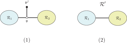
Figure 7. $\mathcal{R}^{\prime}$ in Case 3

∎

4.3. Compatibility of Kuranishi Structures with Forgetful Maps

We next discuss the relation between forgetful maps and Kuranishi structures.

Definition .

Let $\mathfrak{p}\in\mathcal{M}_{k+1}^{\rm RGW}(\beta)$ and $\overline{\mathfrak{p}}=\mathfrak{fg}^{\partial}_{j}(\mathfrak{p})\in\mathcal{M}_{k}^{\rm RGW}(\beta)$. Let $\mathcal{U}_{\mathfrak{p}}=(U_{\mathfrak{p}},E_{\mathfrak{p}},s_{\mathfrak{p}},\psi_{\mathfrak{p}})$ and $\mathcal{U}_{\overline{\mathfrak{p}}}=(U_{\overline{\mathfrak{p}}},E_{\overline{\mathfrak{p}}},s_{\overline{\mathfrak{p}}},\psi_{\overline{\mathfrak{p}}})$ be their Kuranishi charts. We say those Kuranishi charts are compatible with the forgetful map if the following holds.

By shrinking the charts, we may assume $U_{\mathfrak{p}}=V_{\mathfrak{p}}/\Gamma_{\mathfrak{p}}$ and $U_{\overline{\mathfrak{p}}}=V_{\overline{\mathfrak{p}}}/\Gamma_{\overline{\mathfrak{p}}}$, where $V_{\mathfrak{p}}$, $V_{\overline{\mathfrak{p}}}$ are manifolds and $\Gamma_{\mathfrak{p}}$ and $\Gamma_{\overline{\mathfrak{p}}}$ are finite groups acting on them.

1. There exists a group homomorphism $\phi_{\mathfrak{p}}:\Gamma_{\mathfrak{p}}\to\Gamma_{\overline{\mathfrak{p}}}$.

2. There exists a $\phi_{\mathfrak{p}}$ equivariant map

   $$F_{\mathfrak{p}}:V_{\mathfrak{p}}\to V_{\overline{\mathfrak{p}}}$$

   that is a strata-wise smooth submersion.

3. $E_{\mathfrak{p}}$ is isomorphic to the pullback of $E_{\overline{\mathfrak{p}}}$ by $F_{\mathfrak{p}}$. In other words, there exists fiberwise isomorphic lift

   $$\tilde{F}_{\mathfrak{p}}:E_{\mathfrak{p}}\to E_{\overline{\mathfrak{p}}}$$

   of $F_{\mathfrak{p}}$, which is $\phi_{\mathfrak{p}}$ equivariant.

4. $\tilde{F}_{\mathfrak{p}}\circ s_{\mathfrak{p}}=s_{\overline{\mathfrak{p}}}\circ F_{\mathfrak{p}}$.

5. $\psi_{\overline{\mathfrak{p}}}\circ F_{\mathfrak{p}}=\mathfrak{fg}^{\partial}_{j}\circ\psi_{\mathfrak{p}}$ on $s_{\mathfrak{p}}^{-1}(0)$.

6. $\tilde{F}_{\mathfrak{p}},F_{\mathfrak{p}}$ is compatible with the coordinate change in the same sense as in Item (3) of Proposition 2.2.

The same statement holds for (4.9) and (4.10).

Definition .

Let $\mathfrak{u}\in\mathcal{M}_{k+1}^{\rm RGW}(L;\beta)$. Let $\check{R}$ be the very detailed tree describing the combinatorial type of $\mathfrak{u}$. We fix a TSD $\Xi$ at $\mathfrak{u}$. Let $\mathfrak{y}=(\vec{\mathfrak{x}},\vec{\sigma},(u^{\prime}_{v}),(U^{\prime}_{v}),(\rho_{e}),(\rho_{i}))$ be an inconsistent map with respect to $\Xi$.

1. Remove all the edges $e$ of $\check{R}$ with $\sigma_{e}=0$, and let $\check{R}_{0}$ be one of the connected components of the resulting graph. The union of all the spaces $\Sigma_{\mathfrak{y},v}$, where $v$ belongs to $\check{R}_{0}$, is called an irreducible component of $\mathfrak{y}$. If it does not make any confusion, the union of all the interior vertices $v$ of $\check{R}$, which belong to $\check{R}_{0}$, is also called an irreducible component.

2. An irreducible component of $\mathfrak{y}$ is called a trivial component if the following holds:

   1. All the vertices in this component have color ${\rm d}$.

   2. All the homology classes assigned to the vertices in this component are $0$.

3. We say $\mathfrak{y}$ preserves triviality if for any interior vertex $v$ in a trivial component, the map $u^{\prime}_{v}$ is constant.

In this subsection we will construct Kuranishi structures on $\mathcal{M}_{k+1}^{\rm RGW}(L;\beta)$ which are compatible with forgetful map in the sense we defined above.

Lemma .

Given any element $\mathfrak{u}\in\mathcal{M}_{k+1}^{\rm RGW}(L;\beta)$, the Kuranishi neighborhood of $\mathfrak{u}$, constructed in [part2:kura], is contained in the set of inconsistent maps which preserve triviality.

Proof.

Suppose $\Xi$ is a small enough TSD such that we can form the obstruction bundle $E_{\mathfrak{u},\mathscr{F},\Xi}(\mathfrak{y})$ over inconsistent maps $\mathfrak{y}$ with respect to $\Xi$. Let $\Upsilon$ be the TSO given as $(\Xi,\{E_{\mathfrak{u},\mathscr{F},\Xi}\})$. We assume that $\mathfrak{y}$ is chosen such that it represents an element of $\widehat{\mathcal{U}}(\mathfrak{u},\Upsilon)$. If $[\mathfrak{u},\mathfrak{p},\phi]$ is a quasi component of $\mathfrak{u}$, then the image of $\phi$ is away from the components of $\mathfrak{u}$ with trivial homology classes. Consequently, restriction of the obstruction bundle $E_{\mathfrak{u},\mathscr{F},\Xi}(\mathfrak{y})$ to any trivial component of $\mathfrak{y}$ is trivial. Therefore, the restriction of $u_{\mathfrak{y}}$ to any such component has trivial homology class and satisfies the Cauchy-Riemann equation with a trivial obstruction bundle, and hence it is a constant map. ∎

Suppose $\mathfrak{y}$ is an inconsistent map with respect to $\Xi$. Let $\Xi^{\prime}$ be another TSD at the same point $\mathfrak{u}$. If $\Xi^{\prime}$ is small enough, then we obtain a corresponding inconsistent map $\mathfrak{y}^{\prime}$ with respect to $\Xi^{\prime}$. (See the discussion preceding [part2:kura, Lemma 9.22].) It is clear that $\mathfrak{y}$ preserves triviality if and only if $\mathfrak{y}^{\prime}$ preserves triviality.

We form the forgetful map:

(4.12) $$\mathfrak{fgg}:\mathcal{M}^{\rm RGW}_{k+1}(L;\beta)\to\mathcal{M}^{\rm RGW}_{1}(L;\beta)$$

by forgetting the boundary marked points other than the $0$-th one, by composing the forgetful maps defined in Subsection 4.2.

Lemma .

Let $\mathfrak{u}\in\mathcal{M}^{\rm RGW}_{k+1}(L;\beta)$ and $\mathfrak{u}^{\prime}=\mathfrak{fgg}(\mathfrak{u})\in\mathcal{M}_{1}^{\rm RGW}(L;\beta)$. For any TSD $\Xi^{\prime}=(\vec{w}_{\mathfrak{u}^{\prime}},(\mathcal{N}_{\mathfrak{u}^{\prime},v,i}),(\phi_{\mathfrak{u}^{\prime},v}),(\varphi_{\mathfrak{u}^{\prime},v,e}),\delta^{\prime})$ at $\mathfrak{u}^{\prime}$ there is a TSD $\Xi=(\vec{w}_{\mathfrak{u}},(\mathcal{N}_{\mathfrak{u},v,i}),(\phi_{\mathfrak{u},v}),(\varphi_{\mathfrak{u},v,e}),\delta)$ at $\mathfrak{u}$ such that any inconsistent map $\mathfrak{y}$ with respect to $\Xi$ which preserves triviality induces an inconsistent map $\mathfrak{y}^{\prime}$ with respect to $\mathfrak{u}^{\prime}$.

Proof.

Let $\check{R}$ (resp. $\check{R}^{\prime}$) be the very detailed DD-ribbon tree describing the combinatorial type of $\mathfrak{u}$ (resp. $\mathfrak{u}^{\prime}$). By construction we observe that the vertices of $\check{R}$ with color $\rm s$ or $\rm D$ are in one to one correspondence with the vertices of the same color in $\check{R}^{\prime}$. Also the set of vertices of $\check{R}^{\prime}$ with color $\rm d$ is a subset of the vertices of $\check{R}$ with color $\rm d$. The difference $C^{\rm int}_{0}(\check{R})\setminus C^{\rm int}_{0}(\check{R}^{\prime})$ consists of vertices $v$ such that the map $u_{v}$ is constant on it. In particular, for any such vertex $v$, the component $\Sigma_{\mathfrak{u},v}$ together with the marked points and nodal points is already source stable. Therefore, we can require that the additional marked points $\vec{w}_{{\mathfrak{u}}}$ of the TSD $\Xi$ do not belong to such irreducible components of $\Sigma_{\mathfrak{u}}$. Thus we may find marked points $\vec{w}_{\mathfrak{u}}$ on $\Sigma_{\mathfrak{u}^{\prime}}$ such that they are identified with $\vec{w}_{{\mathfrak{u}^{\prime}}}$ using the map $\Sigma_{\mathfrak{u}}\to\Sigma_{\mathfrak{u}^{\prime}}$ which collapses the components associated to $C^{\rm int}_{0}(\check{R})\setminus C^{\rm int}_{0}(\check{R}^{\prime})$. We define $\vec{w}_{\mathfrak{u}}$ to be the set of the additional marked points of $\Xi$. We also assume that the set of transversals of $\Xi$ are identified with that of $\Xi^{\prime}$ in an obvious way.

We also require that the trivialization of the universal families of irreducible components associated to $\Xi$ and to $\Xi^{\prime}$ to be related to each other as follows. For any sphere component we assume that the associated trivializations agree with each other. For $v\in C^{\rm int}_{0}({\check{R}}^{\prime})\subset C^{\rm int}_{0}(\check{R})$ with level $0$, let $\mathcal{M}^{{\rm source}}_{\mathfrak{u},v}$, $\mathcal{M}^{{\rm source}}_{\mathfrak{u}^{\prime},v}$ be the corresponding moduli spaces of marked disks and $\mathcal{C}^{{\rm source}}_{\mathfrak{u},v}\to\mathcal{M}^{{\rm source}}_{\mathfrak{u},v}$, $\mathcal{C}^{{\rm source}}_{\mathfrak{u}^{\prime},v}\to\mathcal{M}^{{\rm source}}_{\mathfrak{u}^{\prime},v}$ be the universal families. We take a trivialization of $\mathcal{C}^{{\rm source}}_{\mathfrak{u},v}$ over a sufficiently small neighborhood $\mathcal{V}_{\mathfrak{u},v}^{{\rm source}}$ of $\Sigma_{\mathfrak{u},v}$ so that the following diagram commutes:

(4.13)

where the vertical arrows are obvious forgetful maps. For the trivializations of the universal families of disk components corresponding to $v\in C^{\rm int}_{0}(\check{R})\setminus C^{\rm int}_{0}(\check{R}^{\prime})$, that are parts of $\Xi$, we take an arbitrary choice.

For $v\in C^{\rm int}_{0}({\check{R}}^{\prime})\subset C^{\rm int}_{0}(\check{R})$ and an edge $e$ incident to $v$, we pick $\varphi_{\mathfrak{u},v,e}$ to be the analytic family induced by $\varphi_{\mathfrak{u}^{\prime},v,e}$. In the case that $v\in C^{\rm int}_{0}({\check{R}})\setminus C^{\rm int}_{0}(\check{R}^{\prime})$, the corresponding component $\Sigma_{\mathfrak{u},v}$ in addition to boundary marked points has at most two boundary nodes. If there are two boundary nodes inducing edges $e_{+}$ and $e_{-}$ incident to $v$, then we can identify $\Sigma_{\mathfrak{u},v}$ with the strip $[0,1]\times{\mathbb{R}}$ where the boundary node associated to $e_{\pm}$ is in correspondence with the point at $\pm\infty$ on the boundary of $[0,1]\times{\mathbb{R}}$. We fix one such identification and let $[0,1]\times[T,\infty)$ and $[0,1]\times(-\infty,-T]$, for a large value of $T$, induce the analytic families of coordinates $\varphi_{\mathfrak{u},v,\pm e}$. In the case that there is only one interior edge incident to $v$, we follow a similar strategy with the difference that we only need to use the half strip $[0,1]\times[T,\infty)$ to define the corresponding analytic family of coordinates. We also let $\delta=\delta^{\prime}$.

Now, let

$$\mathfrak{y}=(\vec{\mathfrak{x}}_{\mathfrak{y}},\vec{\sigma}_{\mathfrak{y}},(u^{\prime}_{{\mathfrak{y}},v}),(U^{\prime}_{{\mathfrak{y}},v}),(\rho_{{\mathfrak{y}},e}),(\rho_{{\mathfrak{y}},i}))$$

be an inconsistent map with respect to $\Xi$ which preserves triviality. We wish to define

$${\mathfrak{y}^{\prime}}=(\vec{\mathfrak{x}}_{\mathfrak{y}^{\prime}},\vec{\sigma}_{{\mathfrak{y}^{\prime}}},(u^{\prime}_{{\mathfrak{y}^{\prime}},v}),(U^{\prime}_{{\mathfrak{y}^{\prime}},v}),(\rho_{{\mathfrak{y}^{\prime}},e}),(\rho_{{\mathfrak{y}^{\prime}},i}))$$

an inconsistent map with respect to $\Xi^{\prime}$. It is clear from the definition of $\Xi$ that there are $\vec{\mathfrak{x}}_{{\mathfrak{y}^{\prime}}},\vec{\sigma}_{{\mathfrak{y}^{\prime}}}$ such that

(4.14) $$\Sigma_{\mathfrak{u}}(\vec{\mathfrak{x}}_{\mathfrak{y}},\vec{\sigma}_{\mathfrak{y}})\cong\Sigma_{{\mathfrak{u}^{\prime}}}(\vec{\mathfrak{x}}_{{\mathfrak{y}^{\prime}}},\vec{\sigma}_{{\mathfrak{y}^{\prime}}}).$$

We take $\rho_{{\mathfrak{y}},e}=\rho_{{\mathfrak{y}^{\prime}},e}$, $\rho_{{\mathfrak{y}},i}=\rho_{{\mathfrak{y}^{\prime}},i}.$ Moreover, $U^{\prime}_{{\mathfrak{y}},v}=U^{\prime}_{{\mathfrak{y}^{\prime}},v}$ and $u^{\prime}_{{\mathfrak{y}},v}=u^{\prime}_{{\mathfrak{y}^{\prime}},v}$ if the color of $v$ is ${\rm s}$.

We consider a disk component $\Sigma_{{\mathfrak{y}^{\prime}},v}$. There exists a unique irreducible component (in the sense of Definition 4.3, where we use $\vec{\sigma}_{{\mathfrak{y}^{\prime}}}$) which contains this component. We denote by $\Sigma^{+}_{\mathfrak{u}^{\prime},v}(\vec{\mathfrak{x}}_{{\mathfrak{y}^{\prime}}},\vec{\sigma}_{{\mathfrak{y}^{\prime}}})$ the union of the disk components contained in this irreducible component. We take the irreducible components of $\mathfrak{y}$ which correspond to it and define $\Sigma^{+}_{{\mathfrak{u}},v}(\vec{\mathfrak{x}}_{{\mathfrak{y}}},\vec{\sigma}_{{\mathfrak{y}}})$ in the same way. By (4.14) we have an isomorphism

(4.15) $$\Sigma^{+}_{\mathfrak{u}^{\prime},v}(\vec{\mathfrak{x}}_{{\mathfrak{y}^{\prime}}},\vec{\sigma}_{{\mathfrak{y}^{\prime}}})\cong\Sigma^{+}_{{\mathfrak{u}},v}(\vec{\mathfrak{x}}_{{\mathfrak{y}}},\vec{\sigma}_{{\mathfrak{y}}}).$$

The maps $u^{\prime}_{\mathfrak{y},v}$ for various $v$ in this irreducible component induces a map

(4.16) $$(\Sigma^{+}_{{\mathfrak{u}},v}(\vec{\mathfrak{x}}_{{\mathfrak{y}}},\vec{\sigma}_{{\mathfrak{y}}}),\partial\Sigma^{+}_{{\mathfrak{u}},v}(\vec{\mathfrak{x}}_{{\mathfrak{y}}},\vec{\sigma}_{{\mathfrak{y}}}))\to(X,L).$$

This map is smooth. (Since $\Sigma^{+}_{{\mathfrak{u}},v}(\vec{\mathfrak{x}}_{{\mathfrak{y}}},\vec{\sigma}_{{\mathfrak{y}}})$ is obtained by gluing along the components associated to the level $0$ edges, the maps $u^{\prime}_{\mathfrak{y},v}$ are consistent on overlaps.) We use (4.15) and (4.16) to define $u^{\prime}_{{\mathfrak{y}^{\prime}},v}$. Using the fact that $\mathfrak{y}$ is an consistent map preserving triviality, it is easy to see that $u^{\prime}_{{\mathfrak{y}^{\prime}},v}$ for various $v$ are consistent at the nodal points corresponding to the level 0 edges $e$ with $\sigma_{{\mathfrak{y}^{\prime}},e}=0$, and ${\mathfrak{y}^{\prime}}=(\vec{\mathfrak{x}}_{\mathfrak{y}^{\prime}},\vec{\sigma}_{{\mathfrak{y}^{\prime}}},(u^{\prime}_{{\mathfrak{y}^{\prime}},v}),(U^{\prime}_{{\mathfrak{y}^{\prime}},v}),(\rho_{{\mathfrak{y}^{\prime}},e}),(\rho_{{\mathfrak{y}^{\prime}},i}))$ is an inconsistent map with respect to $\Xi^{\prime}$. ∎

Remark .

The notion of preserving triviality plays an important role in the proof. The other important point is that we do not put any obstruction bundle on the components where the maps are constant.

Let $\mathfrak{u}$, $\mathfrak{y}$, $\mathfrak{u}^{\prime}$ and $\mathfrak{y}^{\prime}$ be as in Lemma 4.3 and $\check{R}$, $\check{R}^{\prime}$ be the very detailed tree describing the combinatorial types of $\mathfrak{u}$, $\mathfrak{u}^{\prime}$, respectively. We define

$$L^{2}_{m,\delta,{\rm nontri}}(\mathfrak{y},{\mathfrak{u}})= \bigoplus_{v\in C^{\rm int}_{0}(\check{R});c(v)={\rm s}}L^{2}_{m,\delta}(\Sigma^{+}_{\mathfrak{y},v};(u^{\prime}_{\mathfrak{y},v})^{*}TX\otimes\Lambda^{0,1})$$

$$\oplus\bigoplus_{v\in C^{\rm int}_{0}(\check{R});c(v)={\rm D}}L^{2}_{m,\delta}(\Sigma^{+}_{\mathfrak{y},v};(\pi\circ U^{\prime}_{\mathfrak{y},v})^{*}T\mathcal{D}\otimes\Lambda^{0,1})$$

$$\oplus\bigoplus_{v\in C^{\rm int}_{0}(\check{R});c(v)={\rm d},\atop\text{$u^{\prime}_{\mathfrak{y},v}$ is not constant}}L^{2}_{m,\delta}(\Sigma^{+}_{\mathfrak{y},v};(u^{\prime}_{\mathfrak{y},v})^{*}TX\otimes\Lambda^{0,1})$$

$$L^{2}_{m,\delta,{\rm nontri}}({\mathfrak{y}^{\prime}},{\mathfrak{u}^{\prime}})= \bigoplus_{v\in C^{\rm int}_{0}(\check{R}^{\prime});c(v)={\rm s}}L^{2}_{m,\delta}(\Sigma^{-}_{{\mathfrak{y}^{\prime}},v};(u^{\prime}_{{\mathfrak{y}^{\prime}},v})^{*}TX\otimes\Lambda^{0,1})$$

$$\oplus\bigoplus_{v\in C^{\rm int}_{0}(\check{R}^{\prime});c(v)={\rm D}}L^{2}_{m,\delta}(\Sigma^{-}_{{\mathfrak{y}^{\prime}},v};(\pi\circ U^{\prime}_{{\mathfrak{y}^{\prime}},v})^{*}T\mathcal{D}\otimes\Lambda^{0,1})$$

$$\oplus\bigoplus_{v\in C^{\rm int}_{0}(\check{R}^{\prime});c(v)={\rm d},\atop\text{$u^{\prime}_{{\mathfrak{y}^{\prime}},v}$ is not constant}}L^{2}_{m,\delta}(\Sigma^{-}_{{\mathfrak{y}^{\prime}},v};(u^{\prime}_{{\mathfrak{y}^{\prime}},v})^{*}TX\otimes\Lambda^{0,1}).$$

There are canonical identification between the components appearing in the above two formulas. Therefore, there exists a canonical map

(4.17) $$I_{{\mathfrak{y}}\mathfrak{y}^{\prime}}:L^{2}_{m,\delta,{\rm nontri}}(\mathfrak{y}^{\prime},\mathfrak{u}^{\prime})\to L^{2}_{m,\delta,{\rm nontri}}(\mathfrak{y},{\mathfrak{u}}).$$

Definition .

Let $\{E_{\mathfrak{u},\Xi}(\mathfrak{y})\}$ and $\{E_{\mathfrak{u}^{\prime},\Xi^{\prime}}(\mathfrak{y}^{\prime})\}$ be obstruction bundle data for the moduli spaces $\mathcal{M}_{k+1}^{\rm RGW}(L;\beta)$ and $\mathcal{M}_{1}^{\rm RGW}(L;\beta)$, respectively. We say that they are compatible with the forgetful map if

(4.18) $$I_{{\mathfrak{y}}\mathfrak{y}^{\prime}}(E_{\mathfrak{u}^{\prime},\Xi^{\prime}}(\mathfrak{y}^{\prime}))=E_{\mathfrak{u},\Xi}(\mathfrak{y})$$

when $\mathfrak{u}^{\prime}$, $\Xi^{\prime}$, $\mathfrak{y}^{\prime}$ are related to $\mathfrak{u}$, $\Xi$, $\mathfrak{y}$ as in Lemma 4.3.

Definition .

A system of obstruction bundle data for $\{\mathcal{M}_{k+1}^{\rm RGW}(L;\beta)\}_{\omega\cap\beta\leq E}$ is said to be compatible with the forgetful map if Definition 4.3 holds for each of the moduli spaces $\mathcal{M}_{k+1}^{\rm RGW}(L;\beta)$ and $\mathcal{M}_{1}^{\rm RGW}(L;\beta)$ with $\omega\cap\beta\leq E$.

Suppose $\{E_{\mathfrak{u},\Xi}(\mathfrak{y})\}$ is a system of obstruction bundle data for $\{\mathcal{M}_{k+1}^{\rm RGW}(L;\beta)\}_{\omega\cap\beta\leq E}$, which is disk-component-wise and is compatible with forgetful map. Let $\mathfrak{u}$ be an element of $\mathcal{M}_{k+1}^{\rm RGW}(L;\beta)$ and $\mathfrak{u}^{\prime}=\mathfrak{fgg}(\mathfrak{u})$. Suppose $\Xi$, $\Xi^{\prime}$ are TSDs at $\mathfrak{u}$, $\mathfrak{u}^{\prime}$ which are related to each other as in Lemma 4.3. Using Lemmas 4.3 and 4.3 and consistency of obstruction bundle data with the forgetful map, we can define a map:

$$F_{\mathfrak{u}}:\widehat{\mathcal{U}}(\mathfrak{u};\Upsilon)\to\widehat{\mathcal{U}}(\mathfrak{u}^{\prime};\Upsilon^{\prime}).$$

Here $\Upsilon=(\Xi,E_{\mathfrak{u},\Xi})$, $\Upsilon^{\prime}=(\Xi^{\prime},E_{\mathfrak{u}^{\prime},\Xi^{\prime}})$. In the process of forgetting boundary marked points and passing from $\mathfrak{u}$ to $\mathfrak{u}^{\prime}$, we only might collapse disc components. Since the elements of $\Gamma_{\mathfrak{u}}$ and $\Gamma_{\mathfrak{u}^{\prime}}$ act as identity on disc components, the isotropy groups $\Gamma_{\mathfrak{u}}$ and $\Gamma_{\mathfrak{u}^{\prime}}$ are isomorphic. The map $F_{\mathfrak{u}}$ is also $\Gamma_{\mathfrak{u}}$-equivariant.

It is straightforward to lift the map $F_{\mathfrak{u}}$ to a $\Gamma_{\mathfrak{u}}$-equivariant map:

$$\tilde{F}_{\mathfrak{u}}:\mathcal{E}_{\mathfrak{u}}\to\mathcal{E}_{\mathfrak{u}^{\prime}}$$

such that

$$\tilde{F}_{\mathfrak{u}}\circ\mathfrak{s}_{\mathfrak{u}}=\mathfrak{s}_{\mathfrak{u}^{\prime}}\circ F_{\mathfrak{u}},$$

and for any $\mathfrak{y}\in\mathfrak{s}_{\mathfrak{u}}^{-1}(0)/\Gamma_{\mathfrak{u}}$ we have

$$\psi_{\mathfrak{u}^{\prime}}\circ F_{\mathfrak{u}}(\mathfrak{y})=\mathfrak{fgg}\circ\psi_{\mathfrak{u}}(\mathfrak{y})$$

The maps $F_{\mathfrak{u}}$ and $\tilde{F}_{\mathfrak{u}}$ are also compatible with coordinate changes. We can summarize this discussion as follows:

Theorem .

Suppose a system of obstruction bundle data $\{E_{\mathfrak{u},\Xi}(\mathfrak{y})\}$ for moduli spaces $\{\mathcal{M}_{k+1}^{\rm RGW}(L;\beta)\}_{\omega\cap\beta\leq E}$ is disk-component-wise and is compatible with forgetful map. Then the resulting system of Kuranishi structures is compatible at the boundary components and corners (in the sense of Propositions 2.2, 2.2 and 2.2) and compatible with the forgetful map in the sense of Definition 4.3.

Proof.

Compatibility of the forgetful map with Kuranishi structures of moduli spaces $\mathcal{M}_{k+1}^{\rm RGW}(L;\beta)$ is equivalent to the existence of the maps $F_{\mathfrak{u}}$ and $F_{\mathfrak{u}^{\prime}}$ with the above properties. We just need to point out that in Definition 4.3 we consider the map

$$\mathfrak{fg}_{j}^{\partial}:\mathcal{M}_{k+1}^{\rm RGW}(L;\beta)\to\mathcal{M}_{k}^{\rm RGW}(L;\beta).$$

given by forgetting the $j$-th marked point. The proof of a similar result for the map $\mathfrak{fg}_{j}^{\partial}$ is essentially the same. Let $\mathfrak{u}_{1}\in\mathcal{M}_{k+1}^{\rm RGW}(L;\beta)$, $\mathfrak{u}_{2}=\mathfrak{fg}_{j}^{\partial}(\mathfrak{u}_{1})$. Starting with a TSO $\Upsilon_{2}$ at $\mathfrak{u}_{2}$, we can follow the proof of Lemma 4.3 to define a TSO $\Upsilon_{1}$ at $\mathfrak{u}_{1}$, and form a map from $\widehat{\mathcal{U}}(\mathfrak{u}_{1},\Upsilon_{1})$ to $\widehat{\mathcal{U}}(\mathfrak{u}_{2},\Upsilon_{2})$. The remaining properties can be verified in a similar way. ∎

Remark .

In general, one needs to be careful about the differentiability of $F_{\mathfrak{u}}$. The strata-wise smoothness is easy to show by elliptic regularity. The issue of differentiability, when a change of stratum happens, is discussed in [fooobook2, page 778]. This issue is relevant to the application of Theorem 4.3, when we want to pull-back a multi-valued perturbation by the forgetful map.

There are two ways to resolve this issue. First we can consider multi-sections which have exponential decay in the gluing parameter $T$. (We use $T,\theta$ where $\sigma=\exp(-(T+\theta\sqrt{-1}))$.) Even though the forgetful map $F_{\mathfrak{u}}$ may not be smooth, the pull back of a multi-section with exponential decay is a multi-section which is not only smooth but also has an exponential decay. (See also [fooobook2, page 778].)

In our situation discussed in the next subsection, we can use a simpler method to resolve this issue. For the purpose of this paper, we need to pull back a never vanishing multi-section. Thus pulling back the multi-section in $C^{0}$ sense is enough. This is because we need differentiability of the multi-section only in a neighborhood of its zero set.

To complete our construction of a system of Kuranishi structures which is compatible with the forgetful map, it remains to prove the following result.

Lemma .

There exists a system of obstruction bundle data which is disk component wise and is compatible with forgetful map.

Proof.

The proof is essentially the same as the proof in Section 3. As before, we construct the system of obstruction bundle data by induction on $\beta\cap[\omega]$. In each step of the induction, we firstly construct an obstruction bundle data on $\mathcal{M}^{\rm RGW}_{1}(L;\beta)$. This system automatically induces an obstruction bundle data on $\mathcal{M}^{\rm RGW}_{k+1}(L;\beta)$ by requiring Condition (4.18).

To be more detailed, we fix a finite subset $\mathfrak{P}(\beta)$ of $\mathcal{M}_{1}^{\rm RGW}(L;\beta)$ as in (OBI) and a vector space $E_{\mathfrak{p}}$ for $\mathfrak{p}\in\mathfrak{P}(\beta)$ as in (OBII). We also fix spaces $\mathscr{F}_{\beta}$, $\mathscr{F}^{\circ}_{\beta}$ which fixes a set of quasi components for each $\mathfrak{u}\in\mathcal{M}_{1}^{\rm RGW}(L;\beta)$. We require these objects satisfy Conditions 3.3, 3.3, 3.3, 3.3, 3.3. If $\mathfrak{u}\in\mathcal{M}_{k+1}^{\rm RGW}(L;\beta)$, then we define $\mathscr{F}_{\beta}(\mathfrak{u})$, $\mathscr{F}^{\circ}_{\beta}(\mathfrak{u})$ to be $\mathscr{F}_{\beta}(\mathfrak{u}^{\prime})$, $\mathscr{F}^{\circ}_{\beta}(\mathfrak{u}^{\prime})$ where $\mathfrak{u}^{\prime}=\mathfrak{fgg}(\mathfrak{u})$. Since the obstruction bundle data for $\mathcal{M}_{1}^{\rm RGW}(L;\beta)$ satisfies Conditions 3.3, 3.3, 3.3, 3.3 and 3.3 the induced obstruction bundle for $\mathcal{M}_{k+1}^{\rm RGW}(L;\beta)$ satisfies the corresponding conditions. ∎

4.4. Perturbation and forgetful map

We next discuss compatibility of perturbations and forgetful map.

Proposition .

Let $L_{0}$, $L_{1}$ be a pair of transversal compact monotone Lagrangians in $X\setminus\mathcal{D}$ such that their minimal Maslov numbers are $2$. For a positive number $E$, there is a system of multi-valued perturbations $\{\mathfrak{s}_{n}\}$ on the moduli spaces $\mathcal{M}^{\rm RGW}_{k_{1},k_{0}}(L_{1},L_{0};p,q;\beta)$ of virtual dimension $\leq 1$ and $\omega\cap\beta\leq E$ such that:

1. It satisfies Item (1) of Theorem 2.1.

2. The multi-valued perturbations $\{\mathfrak{s}_{n}\}$ are compatible with the description of the boundary given by Propositions 2.2, 2.2 and 2.2.

3. The multi-valued perturbations $\{\mathfrak{s}_{n}\}$ are compatible with the forgetful map of the marked points given by Theorem 4.3.

4. It satisfies Item (3) of Theorem 2.1.

Proof.

For $j=1,\,2$ and $\alpha\in\Pi_{2}(X;L_{j})$ with Maslov index $2$, we fix a multi-valued perturbation on $\mathcal{M}_{1}^{\rm RGW}(L_{j};\alpha)$ such that it induces a transversal multi-valued perturbation on $\mathcal{M}_{1}^{\rm RGW}(L_{j};\alpha;p)$ for any $p\in L_{0}\cap L_{1}$. We extend these multi-valued perturbations to all moduli spaces $\mathcal{M}_{k+1}(L_{j};\alpha)$ in the $C^{0}$ sense such that they are compatible over the boundary in a similar sense as in Theorem 2.1. We use these multi-valued perturbations and induction to define the required multi-valued perturbations on the moduli space $\mathcal{M}^{\rm RGW}_{k_{1},k_{0}}(L_{1},L_{0};p,q;\beta)$. To be more detailed, we construct multi-valued perturbations on $\mathcal{M}^{\rm RGW}_{0,0}(L_{1},L_{0};p,q;\beta)$ by induction on $\omega\cap\beta$. The multi-valued perturbation on the general moduli space $\mathcal{M}^{\rm RGW}_{k_{1},k_{0}}(L_{1},L_{0};p,q;\beta)$ is given by pulling back from $\mathcal{M}^{\rm RGW}_{0,0}(L_{1},L_{0};p,q;\beta)$. Here we use consistency of Kuranishi structures with the forgetful map.

Suppose we have constructed required multi-valued perturbations for $\beta$ with $\beta\cap\omega<\alpha\cap\omega$. We use the induction hypothesis and the constructed multi-valued perturbations for the moduli spaces of discs to define a perturbation on $\partial\mathcal{M}^{\rm RGW}_{0,0}(L_{1},L_{0};p,q;\beta)$ in the same way as in Theorem 2.1. We wish to analyze zeros of our induced multi-section on the boundary of $\mathcal{M}^{\rm RGW}_{0,0}(L_{1},L_{0};p,q;\beta)$. In compare to Theorem 2.1, the new types of zeros are given by disc bubbles with Maslov index $2$. Such boundary components have the form

(4.19) $$\mathcal{M}^{\rm RGW}_{1,0}(L_{1},L_{0};p,q;\beta_{0})\,\hat{\times}_{L_{1}}\,\mathcal{M}_{1}^{\rm RGW}(L_{1};\beta_{1})$$

or

(4.20) $$\mathcal{M}^{\rm RGW}_{0,1}(L_{1},L_{0};p,q;\beta_{0})\,\hat{\times}_{L_{0}}\,\mathcal{M}_{1}^{\rm RGW}(L_{0};\beta_{2}),$$

where $\beta_{0}+\beta_{1}=\alpha$ and the Maslov index of $\beta_{1}$ is $2$. We focus on the boundary components of the form in (4.19). The other case is similar. There are two cases to consider.

(Case 1) ($\beta_{0}\neq 0$): The virtual dimension of $\mathcal{M}^{\rm RGW}_{1,0}(L_{1},L_{0};p,q;\beta_{0})$ is

$$\dim(\mathcal{M}^{\rm RGW}_{0,0}(L_{1},L_{0};p,q;\alpha))-1.$$

If the virtual dimension of $\mathcal{M}^{\rm RGW}_{0,0}(L_{1},L_{0};p,q;\alpha)$ is not greater than $0$, then the multi-section does not vanish on this component. To treat the case that the virtual dimension of $\mathcal{M}^{\rm RGW}_{0,0}(L_{1},L_{0};p,q;\alpha)$ is $1$, note that the multi-section of $\mathcal{M}^{\rm RGW}_{1,0}(L_{1},L_{0};p,q;\beta_{0})$ is the pull-back of the multi-valued perturbation on $\mathcal{M}^{\rm RGW}_{0,0}(L_{1},L_{0};p,q;\beta_{0})$. This latter moduli space has virtual dimension $-1$ and hence the multi-section does not vanish on it. Therefore, the multi-section does not have any zero on the moduli spaces $\mathcal{M}^{\rm RGW}_{1,0}(L_{1},L_{0};p,q;\beta_{0})$ and (4.19).

(Case 2) ($\beta_{0}=0$): In this case, $p=q$ and $\alpha=0\#\beta_{1}$ where $\beta_{1}$ is a homology class in $\Pi_{2}(X;L_{1})$ with Maslov index $2$. Therefore, the corresponding boundary component is identified with $\mathcal{M}_{1}^{\rm RGW}(L_{1};\alpha;p)$ where $p\in L_{0}\cap L_{1}$. We defined a multi-valued perturbation on this moduli space such that its zero set is cut down transversely and consists of isolated points. Now we can proceed as in Theorem 2.1 to complete the construction of multi-valued perturbations. ∎

5. Proof of the Main Theorem

5.1. Floer Homology and Auxiliary Choices

In this subsection, we show that Floer homology is independent of the auxiliary choices which we use in the definition. At the same time, we verify Item (2) of Theorem 1. To achieve these goals, we adapt standard arguments to the present set up.

5.1.1. Hamiltonian Vector Fields and Floer Chain Complexes

Let $L_{0},L_{1}$ be Lagrangian submanifolds of $X\setminus\mathcal{D}$ and $\psi_{H}:X\to X$ be a Hamiltonian diffeomorphism generated by a compactly supported smooth map $H:(X\setminus\mathcal{D})\times[0,1]\to{\mathbb{R}}$. Our next goal is to compare Floer homology groups $HF(L_{1},L_{0};X\setminus\mathcal{D})$ and $HF(L_{1},\psi_{H}(L_{0});X\setminus\mathcal{D})$.

Remark .

In Theorem 1, we state the isomorphism

$$HF(L_{1},L_{0};X\setminus\mathcal{D})\cong HF(\psi_{H^{\prime}}(L_{1}),\psi_{H}(L_{0});X\setminus\mathcal{D}).$$

Namely, we move $L_{1}$ and $L_{0}$ by possibly different Hamiltonian diffeomorphisms. In fact, the isomorphism:

(5.1) $$HF(L_{1},L_{0};X\setminus\mathcal{D})\cong HF(\psi(L_{1}),\psi(L_{0});X\setminus\mathcal{D}),$$

in the case that $L_{0}$, $L_{1}$ are moved by the same symplectic diffeomorphism $\psi$ is easy to prove because the moduli spaces used to define the left hand side of (5.1) with respect to $J$ are isomorphic, as spaces with Kuranishi structures, to the moduli spaces used to define the right hand side with respect to $\psi_{*}J$. Therefore, (5.1) follows from Proposition 5.1.1 below about the independence of Floer homology from the choice of almost complex structure. As a result, to prove Item (2) of Theorem 1, it suffices to consider the case that we only move $L_{0}$ by a Hamiltonian diffeomorphism $\psi_{H}$.

We firstly consider perturbations of holomorphic strips using Hamiltonian vector fields and time dependent almost complex structures. These perturbations will be also useful in Subsection 5.3. Let $H:(X\setminus\mathcal{D})\times[0,1]\to{\mathbb{R}}$ be as above. We put $H_{t}(x)=H(x,t)$ and let $X_{H_{t}}$ be the Hamiltonian vector field associated to $H_{t}$. Let $\mathcal{J}=\{J_{t}\mid t\in[0,1]\}$ be a family of almost complex structures which is parametrized by $[0,1]$. We require that, for each $t$, the almost complex structure $J_{t}$ has the form of the almost complex structures constructed in [part1:top, Subsection 3.2].

We consider the following equation for $u:{\mathbb{R}}\times[0,1]\to X$:

(5.2) $$\frac{\partial u}{\partial\tau}+J_{t}\left(\frac{\partial u}{\partial t}-X_{H_{t}}\right)=0.$$

In order to state the required asymptotic behavior of $u$, we need to replace intersection points $L_{0}\cap L_{1}$ with the following space:

Definition .

Let $R(L_{0},L_{1};H)$ be the set of elements $\gamma\in\Omega(L_{0},L_{1})$ such that

(5.3) $$\frac{d\gamma}{dt}(t)=X_{H_{t}}(\gamma(t)).$$

If $o\in\pi_{0}(\Omega(L_{0},L_{1}))$, we define the subset

$$R(L_{0},L_{1};H;o)=R(L_{0},L_{1};H)\cap\Omega(L_{0},L_{1};o).$$

Hereafter we assume $\psi_{H}(L_{0})$ is transversal to $L_{1}$. It implies that the set $R(L_{0},L_{1};H;o)$ is finite.

For $\gamma_{-},\gamma_{+}\in R(L_{0},L_{1};H;o)$, we define $\Pi_{2}(X;L_{1},L_{0};\gamma_{-},\gamma_{+})$ to be the set of all homology classes of maps $u:{\mathbb{R}}\times[0,1]\to X$ such that $u(\tau,0)\in L_{0}$, $u(\tau,1)\in L_{1}$ and

(5.4) $$\lim_{\tau\to-\infty}u(\tau,t)=\gamma_{-}(t),\qquad\lim_{\tau\to-\infty}u(\tau,t)=\gamma_{+}(t).$$

The definition of homology classes is the same as [part1:top, Definition 2.2].

Definition .

Let $\gamma_{-},\gamma_{+}\in R(L_{0},L_{1};H;o)$, $\beta\in\Pi_{2}(X;L_{1},L_{0};\gamma_{-},\gamma_{+})$. We define

$$\mathcal{M}_{k_{1},k_{0}}^{\rm reg}(L_{1},L_{0};\gamma_{-},\gamma_{+};\beta;H,\mathcal{J};{\bf m})$$

to be the set of all objects $((\Sigma,\vec{z}_{0},\vec{z}_{1},\vec{w}),u)$ satisfying the same condition as [part1:top, Definition 3.80] except the following two points:

1. We require $u$ satisfies (5.2) instead of the Cauchy-Riemann equation.

2. We require (5.4) instead of [part1:top, (3.81)].

We can define its compactification $\mathcal{M}^{\rm RGW}_{k_{1},k_{0}}(L_{1},L_{0};\gamma_{-},\gamma_{+};\beta;H,\mathcal{J})$ in the same way as $\mathcal{M}^{\rm RGW}_{k_{1},k_{0}}(L_{1},L_{0};\gamma_{-},\gamma_{+};\beta)$.

By replacing $\mathcal{M}^{\rm RGW}_{k_{1},k_{0}}(L_{1},L_{0};p,q;\beta)$ with $\mathcal{M}^{\rm RGW}_{k_{1},k_{0}}(L_{1},L_{0};\gamma_{-},\gamma_{+};\beta;H,\mathcal{J})$, we obtain a modified version of Floer chain complex. That is to say, we define:

(5.5) $$CF(L_{1},L_{0};H,\mathcal{J};o)=\bigoplus_{\gamma\in R(L_{0},L_{1};H;o)}{\mathbb{Q}}[\gamma]$$

and

$$\partial([\gamma_{-}])=\sum_{\gamma_{+},\beta}\#\mathcal{M}^{\rm RGW}_{0,0}(L_{1},L_{0};\gamma_{-},\gamma_{+};\beta)[\gamma_{+}],$$

where the sum is taken over all $\gamma_{+},\beta$ such that $\mathcal{M}^{\rm RGW}_{0,0}(L_{1},L_{0};\gamma_{-},\gamma_{+};\beta)$ has dimention 0. (As before we take a system of multi-valued perturbation $\{\widehat{\mathfrak{s}}^{n}\}$ and the boundary operator depends on $\{\widehat{\mathfrak{s}}^{n}\}$ and $n$.)

Let $L_{0},L_{1}$ and $H$ be given such that $\psi_{H}(L_{0})$ is transversal to $L_{1}$. Let $\gamma:[0,1]\to X$ be an element of $\Omega(L_{0},L_{1})$. We define

(5.6) $$(\psi_{H})_{*}(\gamma)(t):=(\psi_{H}^{t}\circ(\psi_{H})^{-1})(\gamma(t)).$$

Here $\psi^{t}_{H}$ is defined by $\psi^{0}_{H}(x)=x$ and

$$\frac{d}{dt}\psi^{t}_{H}(x)=X_{H_{t}}(\psi^{t}_{H}(x)).$$

This construction determines a map:

$$(\psi_{H})_{*}:\Omega(\psi_{H}(L_{0}),L_{1})\to\Omega(L_{0},L_{1}).$$

The map $(\psi_{H})_{*}$ induces an isomorphism:

(5.7) $$\psi_{H}(L_{0})\cap_{(\psi_{H})_{*}(o)}L_{1}\cong R(L_{0},L_{1};H;o).$$

Thus it induce a homomorphism:

(5.8) $$(\psi_{H})_{*}:CF(L_{1},\psi_{H}(L_{0});o)\cong CF(L_{1},L_{0};H,\mathcal{J};(\psi_{H})_{*}(o)).$$

We define

$$(\psi_{H})_{*}:\Pi_{2}(X;L_{1},\psi_{H}(L_{0});o)\to\Pi_{2}(L_{1},L_{0};H;(\psi_{H})_{*}(o))$$

in a similar way.

Lemma .

The map $(\psi_{H})_{*}$ determines the following commutative diagrams.

           

For the proof, see [fooobook, Proof of Lemma 5.10].

Corollary .

If $o\in\pi_{0}(\Omega(\psi_{H}(L_{0}),L_{1}))$ satisfies Condition 2.1 (2), then $(\psi_{H})_{*}(o)\in\pi_{0}(\Omega(L_{0},L_{1}))$ also satisfies the same condition.

We next observe that there exists an isomorphism:

$$\mathcal{M}_{k_{1},k_{0}}^{\rm reg}(L_{1},L_{0};\gamma_{-},\gamma_{+};H,\mathcal{J};(\psi_{H})_{*}(\beta);{\bf m})\cong\mathcal{M}_{k_{1},k_{0}}^{\rm reg}(L_{1},\psi_{H}(L_{0});p,q;\beta;{\bf m})$$

where $p$, $q$ are mapped to $\gamma_{-}$, $\gamma_{+}$ by the isomorphism (5.7). Here $\mathcal{J}=\{J_{t}\mid t\in[0,1]\}$ is defined by $J_{t}=(\psi_{H}^{t})_{*}J$. Using the fact that $\psi_{H}^{t}$ is the identity map in a neighborhood of $\mathcal{D}$ we obtain an isomorphism

$$\mathcal{M}^{\rm RGW}_{k_{1},k_{0}}(L_{1},L_{0};\gamma_{-},\gamma_{+};(\psi_{H})_{*}(\beta);\mathcal{J},H)\cong\mathcal{M}^{\rm RGW}_{k_{1},k_{0}}(L_{1},\psi_{H}(L_{0});p,q;\beta)$$

of the spaces with Kuranishi structure. Thus, if $o\in\pi_{0}(\Omega(L_{0},\psi_{H}(L_{0})))$ satisfies Condition 2.1 (2), then we obtain an isomorphism of chain complexes:

(5.9) $$(\psi_{H})_{*}:(CF(L_{1},\psi_{H}(L_{0});o),\partial)\cong(CF(L_{1},L_{0};H,\mathcal{J};(\psi_{H})_{*}(o))),\partial).$$

Consequently, to prove independence of Floer homology from Hamiltonian isotopies of Lagrangian submanifolds, in the case Condition 2.1 (2) is satisfied, it suffices to prove independence from Hamiltonian perturbations. To be more precise, let $H,H^{\prime}:(X\setminus\mathcal{D})\times[0,1]\to{\mathbb{R}}$ be Hamiltonian functions with compact support. Let $\mathcal{J}=\{J_{t}\mid t\in[0,1]\}$ and $\mathcal{J}^{\prime}=\{J^{\prime}_{t}\mid t\in[0,1]\}$ be 1-parameter families of almost complex structures given as in [part1:top, Subsection 3.2]. Note that as we remarked in [part1:top, Remark 3.9] the set of such almost complex structures has trivial homotopy groups.

Proposition .

If $L_{1},L_{0}$ and $o\in\pi_{0}(\Omega(L_{0},L_{1}))$ satisfies Condition 2.1 then we have an isomorphism

$$HF(L_{1},L_{0};H,\mathcal{J};o)\cong HF(L_{1},L_{0};H^{\prime},\mathcal{J}^{\prime};o).$$

The same holds if Condition 2.1 (2) is satisfied and $\mathfrak{PO}_{L_{0}}(1)=\mathfrak{PO}_{L_{1}}(1)$.

5.1.2. Construction of Continuation Maps

We take a 2-parameter family of compatible almost complex structures $\mathcal{JJ}=\{J_{\tau,t}\mid\tau\in{\mathbb{R}},t\in[0,1]\}$. Let $\mathcal{H}:{\mathbb{R}}\times(X\setminus\mathcal{D})\times[0,1]\to{\mathbb{R}}$ be a smooth function. We assume that the following conditions hold.

Condition .

1. For each $(\tau,t)$, the almost complex structure $J_{\tau,t}$ has the form of the almost complex structures constructed in [part1:top, Subsection 3.2].

2. $J_{\tau,t}=J_{t}$ if $\tau$ is sufficiently small, and $J_{\tau,t}=J^{\prime}_{t}$ if $\tau$ is sufficiently large.

3. There exists a neighborhood $U$ of $\mathcal{D}$ such that $\mathcal{H}(\tau,x,t)=0$ for $x\in U$.

4. $\mathcal{H}(\tau,x,t)=H(x,t)$ if $\tau$ is sufficiently small, and $\mathcal{H}(\tau,x,t)=H^{\prime}(x,t)$ if $\tau$ is sufficiently large.

If these conditions are satisfied, then we say $(\mathcal{JJ},\mathcal{H})$ is a homotopy from $(\mathcal{J},H)$ to $(\mathcal{J}^{\prime},H^{\prime})$.

Definition .

Let $\gamma_{-}\in R(L_{0},L_{1};H)$ and $\gamma_{+}\in R(L_{0},L_{1};H^{\prime})$. We define the moduli space:

$$\mathcal{M}_{k_{1},k_{0}}^{\rm reg}(L_{1},L_{0};\gamma_{-},\gamma_{+};\beta;\mathcal{JJ},\mathcal{H};{\bf m})$$

as the set of all objects $((\Sigma,\vec{z}_{0},\vec{z}_{1},\vec{w}),u)$ satisfying the same condition as [part1:top, Definition 3.80] with the following two differences:

1. We require $u$ satisfies

   (5.10) $$\frac{\partial u}{\partial\tau}+J_{\tau,t}\left(\frac{\partial u}{\partial t}-X_{H_{\tau,t}}\right)=0.$$

   Here $H_{\tau,t}(x)=H(\tau,t,x)$.

2. We require

   (5.11) $$\lim_{\tau\to-\infty}u(\tau,t)=\gamma_{-}(t),\qquad\lim_{\tau\to+\infty}u(\tau,t)=\gamma_{+}(t).$$

Here $\beta$ is a homology class of a map $u$ satisfying (5.11) and $u(\tau,0)\in L_{0}$, $u(\tau,1)\in L_{1}$.

We define:

$$\mathcal{M}_{k_{1},k_{0}}^{\rm reg}(L_{1},L_{0};\gamma_{-},\gamma_{+};\beta;\mathcal{JJ},\mathcal{H})=\mathcal{M}_{k_{1},k_{0}}^{\rm reg}(L_{1},L_{0};\gamma_{-},\gamma_{+};\beta;\mathcal{JJ},\mathcal{H};\emptyset).$$

The space $\mathcal{M}_{k_{1},k_{0}}^{\rm reg}(L_{1},L_{0};\gamma_{-},\gamma_{+};\beta;\mathcal{JJ},\mathcal{H})$ has a compactification, which we denote by $\mathcal{M}^{\rm RGW}_{k_{1},k_{0}}(L_{1},L_{0};\gamma_{-},\gamma_{+};\beta;\mathcal{JJ},\mathcal{H})$. It carries an oriented Kuranishi structure with boundary.

Using this moduli space we define

$$\Phi_{\mathcal{JJ},\mathcal{H}}:CF(L_{1},L_{0};H,\mathcal{J};o)\to CF(L_{1},L_{0};H^{\prime},\mathcal{J}^{\prime};o)$$

by the formula:

$$\Phi_{\mathcal{JJ},\mathcal{H}}([\gamma_{-}])=\sum[(\mathcal{M}^{\rm RGW}_{0,0}(L_{1},L_{0};\gamma_{-},\gamma_{+};\beta;\mathcal{H},\mathcal{JJ}),\widehat{\mathfrak{s}}^{n})][\gamma_{+}].$$

Here the sum is taken over $\gamma_{+}$ and $\beta$ such that

$$\dim\mathcal{M}^{\rm RGW}_{0,0}(L_{1},L_{0};\gamma_{-},\gamma_{+};\beta;\mathcal{H},\mathcal{JJ})=0.$$

Then the description of its boundary implies the next formula in the same way as in many other cases of Floer theory (see, for example, [fooobook, fooonewbook, foooHam]).

(5.12) $$\partial\circ\Phi_{\mathcal{JJ},\mathcal{H}}=\Phi_{\mathcal{JJ},\mathcal{H}}\circ\partial.$$

5.1.3. Construction of Chain Homotopies

Let $\mathcal{J},\mathcal{J}^{\prime},H,H^{\prime}$ be as in the beginning of Subsubsection 5.1.2. Suppose $(\mathcal{JJ},\mathcal{H})$ and $(\mathcal{JJ}^{\prime},\mathcal{H}^{\prime})$ are both homotopies from $(\mathcal{J},H)$ to $(\mathcal{J}^{\prime},H^{\prime})$.

A homotopy from $(\mathcal{JJ},\mathcal{H})$ to $(\mathcal{JJ}^{\prime},\mathcal{H}^{\prime})$ is given by a pair

$$\mathcal{JJJ}=\{J_{\tau,t,s}\mid\tau\in{\mathbb{R}},t,s\in[0,1]\},\hskip 28.45274pt\mathcal{HH}:{\mathbb{R}}\times(X\setminus\mathcal{D})\times[0,1]^{2}\to{\mathbb{R}},$$

such that $J_{\tau,t,0}=J_{\tau,t}$, $J_{\tau,t,1}=J^{\prime}_{\tau,t}$, $\mathcal{HH}(\tau,x,t,0)=\mathcal{H}(\tau,x,t)$, $\mathcal{HH}(\tau,x,t,1)=\mathcal{H}^{\prime}(\tau,x,t)$ and, for each $s\in[0,1]$, the pair $(\mathcal{JJ}_{s},\mathcal{H}_{s})$, defined as $\mathcal{JJ}_{s}=\{J_{\tau,t,s}\}$, $\mathcal{H}_{s}(\tau,x,t)=\mathcal{HH}(\tau,x,t,s)$ is a homotopy from $(\mathcal{J},H)$ to $(\mathcal{J}^{\prime},H^{\prime})$. We define

(5.13) $$\mathcal{M}_{k_{1},k_{0}}^{\rm RGW}(L_{1},L_{0};\gamma_{-},\gamma_{+};\beta;\mathcal{HH},\mathcal{JJJ};{\bf m})$$

$$=\bigcup_{s\in[0,1]}\mathcal{M}_{k_{1},k_{0}}^{\rm RGW}(L_{1},L_{0};\gamma_{-},\gamma_{+};\beta;\mathcal{H}_{s},\mathcal{JJ}_{s};{\bf m})\times\{s\}.$$

This space carries a Kuranishi structure with corners. We define

$$\mathfrak{H}_{\mathcal{JJJ},\mathcal{HH}}:CF(L_{1},L_{0};H,\mathcal{J};o)\to CF(L_{1},L_{0};H^{\prime},\mathcal{J}^{\prime};o)$$

by the formula:

$$\mathfrak{H}_{\mathcal{JJJ},\mathcal{HH}}([\gamma_{-}])=\sum[(\mathcal{M}^{\rm RGW}_{0,0}(L_{1},L_{0};\gamma_{-},\gamma_{+};\beta;\mathcal{HH},\mathcal{JJJ}),\widehat{\mathfrak{s}}^{n})][\gamma_{+}].$$

Here the sum is taken over $\gamma_{+}$ and $\beta$ such that the relevant moduli space is zero dimensional. By studying the boundary of those moduli spaces we have

(5.14) $$\partial\circ\mathfrak{H}_{\mathcal{JJJ},\mathcal{HH}}+\mathfrak{H}_{\mathcal{JJJ},\mathcal{HH}}\circ\partial=\Phi_{\mathcal{JJ}^{\prime},\mathcal{H}^{\prime}}-\Phi_{\mathcal{JJ},\mathcal{H}}.$$

5.1.4. Composition of Continuation Maps

For $i=1,2,3$, let $\mathcal{J}^{(i)},H^{(i)}$ be as in the beginning of Subsubsection 5.1.2. Suppose $(\mathcal{JJ}^{ij},\mathcal{H}^{ij})$ is a homotopy from $(\mathcal{J}^{(i)},H^{(i)})$ to $(\mathcal{J}^{(j)},H^{(j)})$ for $(ij)=(12)$, $(23)$ and $(13)$.

Lemma .

We assume $L_{1},L_{0}$ and $o\in\pi_{0}(\Omega(L_{1},L_{0}))$ satisfy Condition 2.1. Then the composition $\Phi_{\mathcal{JJ}^{23},\mathcal{H}^{23}}\circ\Phi_{\mathcal{JJ}^{12},\mathcal{H}^{12}}$ is chain homotopic to $\Phi_{\mathcal{JJ}^{13},\mathcal{H}^{13}}$. The same holds if we assume $\mathfrak{PO}(L_{1})=\mathfrak{PO}(L_{0})$ instead of Condition 2.1 (1).

Proof.

The proof uses the following family of Hamiltonians:

(5.15) $$\mathcal{H}_{\rho}(\tau,x,t)=\begin{cases}\mathcal{H}^{12}(\tau+T_{0}+\rho,x,t)&\tau\leq 0,\\ \mathcal{H}^{23}(\tau-T_{0}-\rho,x,t)&\tau\geq 0,\end{cases}$$

Since it is similar to standard argument of similar Floer theory we omit it. ∎

Proof of Proposition 5.1.1.

Let $(H,\mathcal{J})$ and $(H^{\prime},\mathcal{J}^{\prime})$ be as in Proposition 5.1.1. We take a homotopy $(\mathcal{H},\mathcal{JJ})$ from $(H,\mathcal{J})$ to $(H^{\prime},\mathcal{J}^{\prime})$ and a homotopy $(\mathcal{H}^{\prime},\mathcal{JJ}^{\prime})$ from $(H^{\prime},\mathcal{J}^{\prime})$ to $(H,\mathcal{J})$. They induce chain maps

$$\Phi_{\mathcal{JJ},\mathcal{H}}:CF(L_{1},L_{0};H,\mathcal{J};o)\to CF(L_{1},L_{0};H^{\prime},\mathcal{J}^{\prime};o),$$

and

$$\Phi_{\mathcal{JJ}^{\prime},\mathcal{H}^{\prime}}:CF(L_{1},L_{0};H^{\prime},\mathcal{J}^{\prime};o)\to CF(L_{1},L_{0};H,\mathcal{J};o).$$

It suffices to show that the compositions $\Phi_{\mathcal{JJ}^{\prime},\mathcal{H}^{\prime}}\circ\Phi_{\mathcal{JJ},\mathcal{H}}$ and $\Phi_{\mathcal{JJ},\mathcal{H}}\circ\Phi_{\mathcal{JJ}^{\prime},\mathcal{H}^{\prime}}$ are homotopic to identity. We take a trivial homotopy $(\mathcal{H}^{0},\mathcal{JJ}^{0})$ from $(H,\mathcal{J})$ to $(H,\mathcal{J})$, namely $\mathcal{H}^{0}_{\tau,t}\equiv H_{t}$ and $\mathcal{JJ}^{0}_{\tau,t}=J_{t}$. By Lemma 5.1.4, it suffices to show that this trivial homotopy induces the identity map. In the case of the trivial homotopy, the space $\mathcal{M}^{\rm RGW}_{0,0}(L_{1},L_{0};\gamma_{-},\gamma_{+};\beta;\mathcal{JJ},\mathcal{H})$ has an ${\mathbb{R}}$ action induced by translations in the $\tau$ direction. This action is free unless $\beta=0$. Therefore, by taking a multi-valued perturbation invariant with respect to this ${\mathbb{R}}$ action, we may assume that the number

$$[\mathcal{M}^{\rm RGW}_{0,0}(L_{1},L_{0};\gamma_{-},\gamma_{+};\beta;\mathcal{H},\mathcal{JJ}),\widehat{\mathfrak{s}}^{n}]$$

is nonzero only if $\beta=0$. For $\beta=0$, the moduli space consists of one point. Thus the chain map induced by the trivial homotopy is an isomorphism. This completes the proof of Proposition 5.1.1. ∎

5.2. Floer Homology with Coefficients in Novikov Rings.

The purpose of this subsection is to remove Condition 2.1 (2) and construct Floer homology over Novikov ring. Note that in Lemma 2.1 we assumed Condition 2.1 (2). So when we remove this condition, Floer’s boundary operator as in Definition 2.1 may not be defined. This is the reason we need to use Novikov ring $\Lambda_{0}^{{\mathbb{Q}}}$. Here $\Lambda_{0}^{{\mathbb{Q}}}$ consists of a formal sum $\sum a_{i}T^{\lambda_{i}}$ such that $a_{i}\in{\mathbb{Q}}$, $\lambda_{i}\geq 0$ and $\lim_{i\to\infty}\lambda_{i}=+\infty$. ($T$ is a formal variable.) We denote by $\Lambda^{{\mathbb{Q}}}$ its field of fractions which consists of similar formal sums but $\lambda_{i}$ can be negative.

We still assume $L_{1}$, $L_{0}$ are monotone in $X\setminus\mathcal{D}$.

Definition .

Let $H:X\setminus\mathcal{D}\to{\mathbb{R}}$ be a compactly supported function. Let $\gamma_{\pm}\in R(L_{0},L_{1};H;o)$ and $\beta\in\Pi_{2}(X;L_{1},L_{0};\gamma_{-},\gamma_{+})$. We define

$$C^{H}(\gamma_{\pm})=H(\gamma_{\pm}(1))=H(\gamma_{\pm}(0))$$

and

(5.16) $$\omega_{H}(\beta)=\int_{{\mathbb{R}}\times[0,1]}u^{*}\omega+C^{H}(\gamma_{+})-C^{H}(\gamma_{-}).$$

Lemma .

If $\mathcal{M}^{\rm RGW}_{k_{1},k_{0}}(L_{1},L_{0};\gamma_{-},\gamma_{+};\beta;H,\mathcal{J})$ is nonempty, then $\omega_{H}(\beta)\geq 0$. It is zero only when $\gamma_{-}=\gamma_{+}$.

Proof.

If $u:{\mathbb{R}}\times[0,1]$ satisfies (5.2) and (5.4), then we can easily show:

$$\int_{{\mathbb{R}}\times[0,1]}u^{*}\omega+C^{H}(\gamma_{+})-C^{H}(\gamma_{-})=\int_{{\mathbb{R}}\times[0,1]}\left\|\frac{\partial u}{\partial\tau}\right\|^{2}dtd\tau.\qed$$

We can use (a variant of) Gromov compactness theorem to show that for each $E$ there exists only a finite number of $\beta$ such that the moduli space $\mathcal{M}^{\rm RGW}_{k_{1},k_{0}}(L_{1},L_{0};\gamma_{-},\gamma_{+};\beta;H,\mathcal{J})$ is nonempty and $\omega_{H}(\beta)\leq E$.

Definition .

Let $L_{1},L_{0}$ be monotone Lagrangian submanifolds of $X\setminus\mathcal{D}$ satisfying $\mathfrak{PO}^{L_{1}}(1)=\mathfrak{PO}^{L_{0}}(1)$. Fix $E$ and choose a system of multi-valued perturbations $\{\mathfrak{s}^{n}\}$ for $\mathcal{M}^{\rm RGW}_{k_{1},k_{0}}(L_{1},L_{0};\gamma_{-},\gamma_{+};\beta;H,\mathcal{J})$ with $\omega_{H}(\beta)\leq E$. We define:

$$\langle\partial_{\beta}[\gamma_{-}],[\gamma_{+}]\rangle=[\mathcal{M}^{\rm RGW}_{0,0}(L_{1},L_{0};\gamma_{-},\gamma_{+};\beta),\mathfrak{s}^{n}]\in{\mathbb{Q}}.$$

for a large enough value of $n$. Then we consider the sum:

(5.17) $$\partial=\sum T^{\omega_{H}(\beta)}\partial_{\beta},$$

which is a $\Lambda_{0}^{{\mathbb{Q}}}$-linear map from $CF(L_{1},L_{0};H,\mathcal{J};o)\otimes_{{\mathbb{Q}}}\Lambda_{0}^{{\mathbb{Q}}}$ to itself of degree $1$.

In the same way as Theorems 2.1 and 4.1 we can prove:

(5.18) $$\partial\circ\partial\equiv\widehat{\mathfrak{PO}}_{L_{1}}(1)-\widehat{\mathfrak{PO}}_{L_{0}}(1)\mod T^{E}.$$

where

$$\widehat{\mathfrak{PO}}_{L}(1)=T^{\omega([\alpha])}[\mathcal{M}^{\rm RGW}(L;\alpha;p),\widehat{\mathfrak{s}}^{n}]\in\Lambda_{0}^{{\mathbb{Q}}}.$$

(Compare with (4.1).)

We thus obtain a chain complex over $\Lambda^{{\mathbb{Q}}}_{0}/T^{E}\Lambda^{{\mathbb{Q}}}_{0}$ under the assumption $\widehat{\mathfrak{PO}}_{L_{1}}(1)=\widehat{\mathfrak{PO}}_{L_{2}}(1)$. We can show this chain complex is independent of the choices of Kuranishi structure and multi-valued perturbation up to chain homotopy equivalence in the same way as Subsection 5.1. We can then use a ‘homotopy inductive limit argument’ similar to [fooobook2, fooonewbook] to obtain a chain complex over the Novikov ring $\Lambda^{{\mathbb{Q}}}_{0}$. Its cohomology is by definition $HF(L_{1},L_{0};o;\Lambda_{0}^{{\mathbb{Q}}};X\setminus\mathcal{D})$. Then in the same way as the proof of Proposition 5.1.1 we can show

$$HF(L_{1},L_{0};H;o;\Lambda_{0}^{{\mathbb{Q}}};X\setminus\mathcal{D})\otimes_{\Lambda_{0}^{{\mathbb{Q}}}}\Lambda^{{\mathbb{Q}}}\cong HF(L_{1},L_{0};H^{\prime};o;\Lambda_{0}^{{\mathbb{Q}}};X\setminus\mathcal{D})\otimes_{\Lambda_{0}^{{\mathbb{Q}}}}\Lambda^{{\mathbb{Q}}}.$$

The argument of this part is the same as [fooobook2, Section 5.3] and so is omitted.

5.3. A Spectral Sequence for $HF(L,\psi_{H}(L);X\setminus\mathcal{D})$

In this subsection we consider the case $L_{0}=\psi_{H}(L_{1})$ and prove part (4) of Theorem 1. More precisely, we prove the following.

Proposition .

Suppose $L\subset X\setminus\mathcal{D}$ is a compact, connected, monotone and spin Lagrangian. Let $H:(X\setminus\mathcal{D})\times[0,1]\to{\mathbb{R}}$ be a compactly supported time dependent Hamiltonian which generates a Hamiltonian diffeomorphism $\psi_{H}:X\to X$. We assume $L_{1}=L$ and $L_{0}=\psi_{H}(L)$ intersect transversely. Then there exists $o_{0}\in\pi_{0}(\Omega(L_{0},L_{1}))$ with the following properties.

1. If $o\neq o_{0}$, then the Floer homology group $HF(L_{1},L_{0};o;\Lambda^{{\mathbb{Q}}};X\setminus\mathcal{D})$ is zero.

2. $o_{0}$ satisfies Condition 2.1 (2) and so we can define the Floer homology group $HF(L_{1},L_{0};o_{0};{{\mathbb{Q}}};X\setminus\mathcal{D})$.

3. There exists a spectral sequence whose $E_{2}$ page is $H_{*}(L;{\mathbb{Q}})$ and which converges to $HF(L_{1},L_{0};o_{0};{{\mathbb{Q}}};X\setminus\mathcal{D})$.

Proof.

Because of the invariance of Floer homology with respect to Hamiltonian isotopies, it suffices to prove this proposition for a specific choice of $H$. There is a symplectomorphism $\Phi$ from a neighborhood $\mathcal{U}$ of $L$ in $X$, disjoint from a neighborhood of $\mathcal{D}$, to a neighborhood of the zero section in $T^{*}L$. Using this symplectomorphism, we define $H$ to be the function

$$H(x,t):=f\circ\pi_{L}(x)\cdot\chi(|x|),$$

where $f:L\to{\mathbb{R}}$ is a Morse-Smale function with respect to the metric induced by $J_{0}$ and $\omega$, $\pi_{L}:T^{*}L\to L$ is the projection map, $|x|$ is the fiber-wise norm of an element of $T^{*}L$ and $\chi:{\mathbb{R}}_{\geq 0}\to[0,1]$ is a function which is equal to $1$ in neighborhood of $0$ and is equal to $0$ for large enough values in ${\mathbb{R}}_{\geq 0}$. An appropriate choice of $\chi$ allows us to regard the above function as a function on $X$. We also assume that the $C^{2}$ norm of $f$ is very small.

The assumption on the $C^{2}$ norm of $f$ implies that $L_{0}\subset\mathcal{U}$ and $\Phi(L)$ can be identified with the graph of $df$ in $T^{*}L$. In particular, the elements of $L_{0}\cap L_{1}$ can be identified with the critical points of $f$. We let $\mu_{f}$ denote the function on $L_{0}\cap L_{1}$ which associates to each intersection point of $L_{0}$ and $L_{1}$ the Morse index of the corresponding critical point. Let $o_{0}$ be the element of $\pi_{0}(\Omega(L_{0},L_{1}))$ that is mapped by $(\psi_{H})_{*}$ to the connected component of the constant maps of $\Omega(L,L)$. Then it is clear that all the elements of $L_{0}\cap L_{1}$ represent $o_{0}$. In particular, $HF(L_{1},L_{0};o;\Lambda^{{\mathbb{Q}}};X\setminus\mathcal{D})$ is trivial unless $o=o_{0}$.

In order to prove (2), it suffices to show that there is a positive constant $c$ such that if $u:S^{1}\times[0,1]\to X$ is a map representing an element of $\pi_{1}(\Omega(L,L;o_{0}))$, then $\omega(u)=c\mu(u)$. We may assume that $u(0,t)$ is independent of $t$. (This is because $o_{0}$ is the component containing the constant paths.) Therefore, $u$ is induced by a map $(D^{2},\partial D^{2})\to(X,L)$. Thus Condition 2.1 (2) follows from the monotonicity of $L$.

Suppose $p,q\in L_{0}\cap L_{1}$ and $u:{\mathbb{R}}\times[0,1]\to X$ is a map representing an element of $\mathcal{M}^{\rm RGW}_{0,0}(L_{1},L_{0};p,q;\beta;\mathcal{J})$. If the image of this map is contained in $\mathcal{U}$, then it is a standard result that $\omega(\beta)=f(p)-f(q)$ and $\mu(\beta)=\mu_{f}(p)-\mu_{f}(q)$. It is shown in [Flo89] that $u(1,\cdot)$ defines a downward gradient flow line of the map $f$. Moreover, this gives a correspondence between the moduli space $\mathcal{M}^{\rm RGW}_{0,0}(L_{1},L_{0};p,q;\beta;\mathcal{J})$ and the moduli space of unparametrized downward gradient flow lines from $p$ to $q$. (Here we need the assumption that $f$ is small in the $C^{2}$ norm.) Next, let $u$ be a map whose image is not contained in $\mathcal{U}$. Using Gromov compactness theorem and the assumption on the size of $f$, it is easy to show that there is a constant $e$, independent of $u$, such that $\omega(\beta)\geq e$. Lemma 2.1 implies that there is an even integer $m$ such that

$$\mu(\beta)=\mu_{f}(p)-\mu_{f}(q)+m,\hskip 56.9055pt\omega(\beta)=f(p)-f(q)+c\cdot m,$$

where $c$ is the monotonicity constant of $L$. Since the $C^{0}$ norm of $f$ is small, the constant $m$ has to be positive.

The previous paragraph implies that the coefficient of $q$ in $\partial p$ is non-zero only if:

$$\mu_{f}(q)-\mu_{f}(p)\geq-1$$

and if the equality holds, then $\langle\partial p,q\rangle$ is equal to the number of unparametrized downward gradient flow lines from $p$ to $q$. (To be more precise, we need to arrange for a multi-valued perturbation produced by Theorem 2.1 which is trivial in the case that $\mu(\beta)=\mu_{f}(p)-\mu_{f}(q)=1$. Since $f$ is a Morse-Smale function, it is easy to see from the proof of Theorem 2.1 that it is possible to arrange for such a multi-valued perturbation.) Therefore, we have

$$CF(L_{1},L_{0};{\mathbb{Q}};o_{0})=\bigoplus_{d}C_{d},\hskip 28.45274pt\partial=\sum_{k=0}^{\infty}\partial_{k},$$

where $C_{d}$ is generated by the elements of $L_{0}\cap L_{1}$ whose Morse index is equal to $d$, and the degree of $\partial_{k}$ with respect to this grading is equal to $-1+2k$. Now we can conclude Part (3) of the proposition from Lemma 5.3. ∎

Lemma .

Let $C$ be a finite dimensional graded vector space and

(5.19) $$\widehat{\partial}=\sum_{k=0}^{\infty}\partial_{k}$$

be a liner map $C\to C$ such that $\partial_{k}$ has degree $-1+2k$ and $\widehat{\partial}\circ\widehat{\partial}=0$. Then there exists a spectral sequence whose $E_{2}$ page is $H(C,\partial_{0})$ and which converges to $H(C;\widehat{\partial})$.

We remark that the sum in (5.19) is actually a finite sum. We also remark that $\partial_{0}\circ\partial_{0}=0$ follows from $\widehat{\partial}\circ\widehat{\partial}=0$.

Proof.

Let

$$(\mathfrak{F}_{\ell}C)_{d}=\begin{cases}C_{d}&\text{if $d>\ell$,}\\ {\rm Im}\,\partial_{0}\cap C_{d}&\text{if $d=\ell$,}\\ 0&\text{if $d<\ell$.}\end{cases}$$

Here $C_{d}$ is the degree $d$ part of $C$. Since $\partial_{k}=0$ for $k<0$, $\mathfrak{F}_{\ell}C$ defines a sub-complex of $C$. Let:

$$\left(\frac{\mathfrak{F}_{\ell}C}{\mathfrak{F}_{\ell+1}C},\overline{\partial}\right)$$

be the graded complex of the filtration determined by the sub-complexes $\mathfrak{F}_{\ell}C$. In particular, there is a spectral sequence with the $E_{2}$ page:

(5.20) $$\bigoplus_{\ell}H\left(\frac{\mathfrak{F}_{\ell}C}{\mathfrak{F}_{\ell+1}C},\overline{\widehat{\partial}}\right)$$

that converges to $H(C;\widehat{\partial})$. It is easy to see that (5.20) is isomorphic to $H(C,\partial_{0})$ ∎

6. Possible Generalizations

In this section, we describe various possible generalizations of the results of this paper. We are planing to come back to some of these directions elsewhere. In particular, we believe that modifications of the method of the present series of papers can be applied to prove many of the conjectures stated here.

6.1. $A_{\infty}$-Structures

Suppose $(X,\omega)$ and $\mathcal{D}$ are as in the beginning of the introduction. Let $L\subset X\setminus\mathcal{D}$ be a relatively spin compact Lagrangian submanifold of $X\setminus\mathcal{D}$.

Conjecture .

There exists a curved filtered $A_{\infty}$-algebra, denoted by $(H^{*}(L;\Lambda^{{\mathbb{Q}}}_{0}),\{\mathfrak{m}_{k}\mid k=0,1,2\dots\})$, on the cohomology group $H^{*}(L;\Lambda^{{\mathbb{Q}}}_{0})$ with Novikov ring coefficients. This $A_{\infty}$-algebra is independent of various choices such as almost complex structures up to homotopy equivalence. If $L$ is monotone, then by putting $T=1$, the element $\mathfrak{m}_{0}(1)\in H^{0}(L;\Lambda^{{\mathbb{Q}}}_{0})$ becomes $\mathfrak{PO}_{L}(1)1,$ where $\mathfrak{PO}_{L}$ is as in Definition 4.1 and $1\in H^{0}(L;\Lambda^{{\mathbb{Q}}}_{0})$ is the unit.

See, for example, [fu2017, Section 2] for the notion of curved filtered $A_{\infty}$-categories and $A_{\infty}$-algebras.

Let $\Lambda^{{\mathbb{Q}}}_{+}$ be the subring of $\Lambda^{{\mathbb{Q}}}_{0}$ consisting of the sums $\sum a_{i}T^{\lambda_{i}}$ with $\lambda_{i}>0$. We call $b\in H^{\rm even}(L;\Lambda^{{\mathbb{Q}}}_{+})$ a weak bounding cochain if

(6.1) $$\sum_{k=0}^{\infty}\mathfrak{m}_{k}(b,\dots,b)\in H^{0}(L;\Lambda^{{\mathbb{Q}}}_{0})$$

and define $\mathfrak{PO}(L;b)\in\Lambda_{+}^{{\mathbb{Q}}}$ by

$$\sum_{k=0}^{\infty}\mathfrak{m}_{k}(b,\dots,b)=\mathfrak{PO}(L;b)1.$$

Let $\mathfrak{L}=\{L_{i}\mid i=1,\dots,N\}$ be a finite set of relatively spin compact Lagrangian submanifolds of $X\setminus\mathcal{D}$ such that $L_{i}$ is transversal to $L_{j}$ for $i\neq j$.

Conjecture .

For each $c\in\Lambda_{+}^{{\mathbb{Q}}}$, there exists a filtered $A_{\infty}$-category $\mathfrak{Fuks}(X\setminus\mathcal{D};c;\mathfrak{L})$ with the following properties:

1. An object of $\mathfrak{Fuks}(X\setminus\mathcal{D};c;\mathfrak{L})$ is a pair $(L_{i},b)$ where $L_{i}\in\mathfrak{L}$ and $b$ is a weak bounding cochain of $L_{i}$ with $\mathfrak{PO}(L_{i};b)=c$.

2. The set of morphisms $CF((L_{i},b),(L_{i},b))$ is an $A_{\infty}$-algebra which is not curved. The $A_{\infty}$ operations of this $A_{\infty}$-algebra are given by

   $$\mathfrak{m}^{\prime}_{k}(x_{1},\dots,x_{k})=\sum_{\ell_{0},\dots,\ell_{k}=0}^{\infty}\mathfrak{m}_{k+\sum\ell_{i}}(b^{\ell_{0}},x_{1},b^{\ell_{1}},\dots,b^{\ell_{k-1}},x_{k},b^{\ell_{k}}).$$

   where $\mathfrak{m}_{*}$ is given in Conjecture 6.1.

3. If $L_{i}$ is monotone and $c=\mathfrak{PO}(L_{i})$ for $i=1,2$, then $(L_{i},0)$ is an object of $\mathfrak{Fuks}(X\setminus\mathcal{D};c;\mathfrak{L})$ for $i=1,2$. The homology group $H_{*}(CF((L_{1},0),(L_{2},0));\mathfrak{m}_{1})$ agrees with the Floer cohomology of Theorem 1.

Conjecture 6.1 can be proved using (the system of) Kuranishi structures on the moduli spaces $\mathcal{M}_{k+1}^{\rm RGW}(L;\beta)$ produced in [part2:kura]. However, in this situation, we need to study moduli spaces whose virtual dimension is higher than one. If $\Lambda^{{\mathbb{Q}}}_{0}$ is the coefficient ring, then we may use singular homology as a chain model for the cohomology of $L$ analogous to [fooobook2, Chapter 7]. If $\Lambda^{{\mathbb{R}}}_{0}$ is the coefficient ring, then we may use de Rham cohomology as a chain model for the cohomology of $L$ analogous to [fooonewbook, Chapters 21 and 22]. To use de Rham cohomology, we also need smoothness of the coordinate change maps of Kuranishi structures. The moduli spaces of pseudo-holomorphic polygons and their RGW-compactifications would be also the main ingredient to prove Conjecture 6.1. See, for example, [fu2017, Section 3].

6.2. Normal Crossing Divisor

Let $(X,\omega)$ be a compact symplectic manifold. Let

(6.2) $$\mathcal{D}=\bigcup_{i=1}^{m}\mathcal{D}_{i}.$$

For $I=\{i_{1},\dots,i_{|I|}\}\subseteq\{1,\dots,m\}$, we define

(6.3) $$\mathcal{D}_{I}=\bigcap_{j=1}^{|I|}\mathcal{D}_{i_{j}}.$$

Then $\mathcal{D}$ is a normal crossing divisor if it satisfies the following properties (see [FMZ:NC]):

1. Each $\mathcal{D}_{i}$ is a codimension 2 smooth symplectic submanifold of $(X,\omega)$.

2. The intersection (6.3) is transversal.

3. The restriction of $\omega$ to $\mathcal{D}_{I}$ defines a symplectic structure on it.

For a compact and relatively spin Lagrangian submanifold $L$ in $X\setminus\mathcal{D}$, we can define the monotonicity of $L$ in $X\setminus\mathcal{D}$ and minimal Maslov number of $L\subset X\setminus\mathcal{D}$ in the same way as in the case that $\mathcal{D}$ is a smooth divisor.

We consider the homology classes $\beta\in H_{2}(X,L;{\mathbb{Z}})$ such that $\beta\cap[\mathcal{D}_{i}]=0$ for all $i$. Then it is reasonable to expect that there is an RGW-type compactification $\mathcal{M}^{\rm reg}_{k+1}(L;\beta)$ of the moduli space of pseudo-holomorphic disks $u:(D^{2},\partial D^{2})\to(X,L)$ of homology class $\beta$. This compactification would be useful to address the following conjecture.

Conjecture .

Theorem 1, Conjectures 6.1 and 6.1 can be generalized to this setup.

For each $I$, there exists a local ${\mathbb{C}}_{*}^{|I|}$ action on a neighborhood of $\mathcal{D}_{I}$. Under the assumption (mc.1)-(mc.3), we can modify the construction of compatible almost complex structure $J$ in [part1:top, Subsection 3.2] so that on a neighborhood $U(I)$ of $\mathcal{D}_{I}$, the almost complex structure is invariant under the local ${\mathbb{C}}_{*}^{|I|}$ action.

The projectivization of the normal bundle $\mathcal{N}_{\mathcal{D}_{i_{j}}}(X)$ defines a ${\bf P}^{1}$-bundle on $\mathcal{D}_{I}$ for each $j$. Therefore, we can form a $({\bf P}^{1})^{|I|}$-bundle on $\mathcal{D}_{I}$. (The fiber is a direct product of $|I|$ copies of ${\bf P}^{1}$.) Using this $({\bf P}^{1})^{|I|}$-bundle for various $I$, instead of the ${\bf P}^{1}$ bundle ${\bf P}(\mathcal{N}_{\mathcal{D}}(X)\oplus{\mathbb{C}})$, we can generalize the constructions in [part1:top] to define RGW-compactification of $\mathcal{M}^{\rm reg}_{k+1}(L;\beta)$. The main difference is that here we need to use $m$ level functions, one level function for each of the irreducible components of $\mathcal{D}$. We also need to use $m$-multiplicity functions. Then one should be able to generalize the construction of [part2:kura] to obtain a system of Kuranishi structures on the RGW-compactifications of $\mathcal{M}^{\rm reg}_{k+1}(L;\beta)$ and generalize the argument of Section 5 to prove an analogue of Theorem 1 in this setup. A corresponding compactification in the context of relative Gromov-Witten theory is developed in [T].

Remark .

In general, a normal crossing divisor $\mathcal{D}$ may not have a decomposition as in (6.2) as some irreducible components may have self intersection. When we stratify $\mathcal{D}$ in a similar way, the bundle which corresponds to the above $({\bf P}^{1})^{|I|}$-bundle still exists. However, there may exist a nontrivial monodromy which exchange the factors. In this case, several level functions may have various symmetries. Therefore, one needs a more careful argument to handle this case. However, we expect that the same conclusion holds for such normal crossing divisors, too.

Remark .

A conjecture similar to Conjecture 6.2 was proposed by M. Gross in a talk in 2016.

6.3. Group Actions on $X$

Let $(X,\omega)$ be a compact symplectic manifold on which a compact Lie group $G$ acts, preserving the symplectic structure. Let $\mathcal{D}\subset X$ be a submanifold as in the beginning of the introduction. We assume $\mathcal{D}$ is $G$-invariant and the almost complex structure $J$ is also $G$-invariant.

Conjecture .

Let $L_{0},L_{1}$ be compact, monotone and relatively spin Lagrangian submanifolds of $X\setminus\mathcal{D}$ which are $G$-invariant. We assume (a) or (b) of Theorem 1 holds. Then there is a $G$-equivariant Lagrangian Floer cohomology group $HF^{G}(L_{1},L_{0};X\setminus\mathcal{D})$, which is a $H^{*}(BG;\Lambda^{{\mathbb{R}}})$-module and has the following properties.

1. If $L_{1}$ and $L_{0}$ have clean intersections, then there exists a spectral sequence converging to $HF^{G}(L_{1},L_{0};X\setminus\mathcal{D})$ such that the $E_{2}$ page of this spectral sequence is the $G$-equivariant cohomology group:

   $$H^{G}(L_{1}\cap L_{0};\Theta\otimes\Lambda^{{\mathbb{R}}}).$$

   Here $\Theta$ is an appropriate ${\mathbb{Z}}_{2}$ local system.

2. It is invariant under $G$-equivariant Hamiltonian isotopies applied to $L_{0}$ and $L_{1}$.

The same claim holds if $\mathcal{D}$ is a normal crossing divisor, namely, the case which is discussed in Subsection 6.2. There is also a filtered $A_{\infty}$-category for a finite set of $G$-invariant, compact and relatively spin Lagrangian submanifolds in $X\setminus\mathcal{D}$, in a similar way as in Conjectures 6.1 and 6.1.

As we mentioned in the introduction and in [DF], we can use Conjecture 6.3 in the case that $X$ is a symplectic cut of the extended moduli space to formulate the symplectic side of the Atiyah-Floer conjecture.

6.4. Non-compact Lagrangians

In this series of papers, we studied compact Lagrangians in the divisor complement. It is natural to generalize this story to the following situation. Let $\overline{L}$ be a submanifold with boundary $\partial L$ such that $\partial L=\overline{L}\cap\mathcal{D}$. Put $L=\overline{L}\setminus\partial L$. We assume $L$ is a Lagrangian submanifold of $X\setminus\mathcal{D}$, and $\partial L$ is a Lagrangian submanifold of $\mathcal{D}$. We also assume that $L$ is invariant under the local ${\mathbb{R}}_{+}$ action induced by the local ${\mathbb{C}}_{*}$ action in a neighborhood of $\mathcal{D}$. Let $\overline{L}_{i}$ ($i=0,1$) be a pair of such Lagrangians. We assume $\partial L_{0}$, $\partial L_{1}$ (resp. $L_{0}$, $L_{1}$) intersect transversally in $\mathcal{D}$ (resp. $X\setminus\mathcal{D}$). We want to define a Floer homology $HF(L_{0},L_{1})$ between such pairs (under appropriate assumptions).

The first observation is that the free abelian group generated by the intersection points $L_{0}\cap L_{1}$ is not an appropriate underlying chain group for this version of Lagrangian Floer homology, unless we assume a certain positivity condition on the divisor. To see this, fix $p,q\in L_{0}\cap L_{1}$ and consider a moduli space $\mathcal{M}(p,q;\beta)$ of pseudo-holomorphic strips with boundary on $L_{0},L_{1}$ and asymptotic to $p,q$ that has (virtual) dimension one. One would expect that studying such moduli spaces can be used to define an appropriate version of Floer’s boundary operator, which is a differential. In addition to the boundary configuration appearing in Theorem 2.1, there is another type of codimension one boundary stratum.

This new configuration can be described as the product of three types of moduli spaces

(6.4) $$\mathcal{M}(p,x;\beta_{1})\times\mathcal{M}(x,y;\beta_{2})\times\mathcal{M}(y,q;\beta_{3}),$$

where $x,y\in\partial L_{0}\cap\partial L_{1}$, $\mathcal{M}(p,x;\beta_{1})$ (resp. $\mathcal{M}(y,q;\beta_{3})$) is the moduli space of pseudo-holomorphic strips bounding $L_{0}$ and $L_{1}$ and asymptotic to $p$ and $x$ (resp. $y$ and $q$), and $\mathcal{M}(x,y;\beta_{2})$ is the moduli spaces of pseudo-holomorphic strips in $\mathcal{D}$, bounding $\partial L_{0}$ and $\partial L_{1}$ and asymptotic to $x$ and $y$ (see Figure 8). We also make the remark that for any element $u$ of $\mathcal{M}(p,x;\beta_{1})$, we can consider the paths $\gamma_{\tau}:=u(\tau,\cdot)$, and as $\tau$ goes to infinity this gives rise to a path from the ray $T_{x}L_{0}/T_{x}\partial L_{0}$ to the ray $T_{x}L_{1}/T_{x}\partial L_{0}$ inside the fiber of the normal bundle of $\mathcal{D}$ at the point $x$. In fact, this path goes in the clockwise direction and the set of homotopy classes of all such paths can be parametrized by non-negative integers. This can be regarded as the relative version of the fact that for our choices of almost complex structure, any intersection point of a pseudo-holomorphic with $\mathcal{D}$ has positive multiplicity. A similar comment applies to the elements of the moduli space $\mathcal{M}(y,q;\beta_{3})$.

Although pseudo-holomorphic curves as in (6.4) with two boundary nodes appear in the union of the codimension 2 strata of the stable map compactification, by a similar argument as in [part2:kura] in the case of pseudo-holomorphic spheres, we can see that such the configuration in (6.4) form codimension 1 strata in the natural adaptation of the RGW compactification to the present setup. This suggests that we need to include the intersection points $\partial L_{0}\cap\partial L_{1}$ in the definition of the chain complex. More precisely, we expect that the chain complex defining $HF(L_{0},L_{1})$ has the form of the abelian group

(6.5) $$\bigoplus_{p\in L_{0}\cap L_{1}}{\mathbb{Q}}\oplus\bigoplus_{x\in\partial L_{0}\cap\partial L_{1}}{\mathbb{Q}}[t].$$

Here $t$ is a formal parameter, and ${\mathbb{Q}}[t]$ is the polynomial ring with rational coefficients. The powers of $t$ are used to keep track of the winding numbers of pseudo-holomorphic curves around points of $\partial L_{0}\cap\partial L_{1}$, which we know that are always in the clockwise direction by the discussion of the previous paragraph.

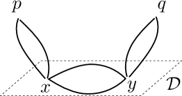
Figure 8. A new type of boundary component

The structure of the above Floer complex is reminiscent of $S^{1}$-equivariant complexes, and one should regard each summand ${\mathbb{Q}}[t]$ as the cohomology of the classifying space $BS^{1}$ of $S^{1}$. In fact, one can justify the appearance of Floer complexes as in (6.5) using Kronheimer and Mrowka’s framework for $S^{1}$-equivariant Floer homology in [km:monopole] (where they use their setup in the context of monopole Floer homology). Lagrangian Floer homology can be regarded as the Morse homology of the action functional on the path space $\Omega(L_{0},L_{1})$ of Lagrangians $L_{0}$ and $L_{1}$. The partial ${\mathbb{C}}_{*}$-action on a neighborhood $\mathfrak{U}$ of $\mathcal{D}$ induces an action of ${\mathbb{C}}_{*}$ on the subspace of $\Omega(L_{0},L_{1})$ given by paths from $L_{0}$ to $L_{1}$ that are contained in $\mathfrak{U}$. In particular, paths into $\mathcal{D}$ are fixed by this action, and we can take the real blow up of the space of all such paths in $\Omega(L_{0},L_{1})$ following [km:monopole]. After lifting the action functional to this blown up space, the Floer complex of this functional has (6.5) as its underlying chain group. In fact, one expects that there is another flavor of the above complex $HF^{\prime}(L_{0},L_{1})$ such that $HF(L_{0},L_{1})$, $HF^{\prime}(L_{0},L_{1})$ and some twisted version of Lagrangian Floer homology of $\partial L_{0}$ and $\partial L_{1}$ form an exact triangle similar to the exact triangle that the three flavors $\widehat{HM}$, $\widecheck{HM}$ and $\overline{HM}$ of monopole Floer homology fit into [km:monopole].

A further generalization of the above direction is obtained by considering non-compact Lagrangians for normal crossing divisors as in Subsection 6.2. In this setup, we may consider $\overline{L}\subset X$, which is a submanifold with boundary and corners, where its codimension $k$ corner consists of the union of $\overline{L}\cap\mathcal{D}_{I}$ with $|I|=k$.