compat=1.0.0

Nikhef-2022-015

Theoretical interpretations of particle physics data, such as the determination of the Wilson coefficients of the Standard Model Effective Field Theory (SMEFT), often involve the inference of multiple parameters from a global dataset. Optimizing such interpretations requires the identification of observables that exhibit the highest possible sensitivity to the underlying theory parameters. In this work we develop a flexible open source framework, ML4EFT, enabling the integration of unbinned multivariate observables into global SMEFT fits. As compared to traditional measurements, such observables enhance the sensitivity to the theory parameters by preventing the information loss incurred when binning in a subset of final-state kinematic variables. Our strategy combines machine learning regression and classification techniques to parameterize high-dimensional likelihood ratios, using the Monte Carlo replica method to estimate and propagate methodological uncertainties. As a proof of concept we construct unbinned multivariate observables for top-quark pair and Higgs+$Z$ production at the LHC, demonstrate their impact on the SMEFT parameter space as compared to binned measurements, and study the improved constraints associated to multivariate inputs. Since the number of neural networks to be trained scales quadratically with the number of parameters and can be fully parallelized, the ML4EFT framework is well-suited to construct unbinned multivariate observables which depend on up to tens of EFT coefficients, as required in global fits.

1 Introduction

The extensive characterization of the Higgs boson properties achieved at the LHC [1, 2, 3] following the tenth anniversary of its discovery [4, 5] represents a powerful example of the unique potential that precision measurements have in unveiling hypothetical signals of beyond the Standard Model (BSM) physics in high-energy collisions. This potential motivates ongoing efforts within the theory and experimental communities to develop novel frameworks, tools, and analysis techniques that enhance the sensitivity of precision LHC measurements to BSM signals in comparison with more traditional approaches.

Since the early days of quantum field theory, effective field theories (EFTs) have proven a robust framework to describe the low-energy limits of theories whose ultraviolet completions are either unknown or with which the computation of predictions is too challenging. Of particular relevance for the model-independent interpretation of LHC measurements is the Standard Model effective field theory (SMEFT) [6, 7, 8] (see also the reviews in [9, 10, 11, 12, 13]), which extends the SM while preserving its (exact) symmetries and its field content. In order to maximize the constraining power of this framework and explore the broadest possible region in the parameter space, it is advantageous to integrate the information contained in different types of processes within a coherent global SMEFT analysis. Several groups have presented combined SMEFT interpretations of LHC data from the Higgs, top-quark, and electroweak sectors, eventually complemented with the information from low-energy electroweak precision observables (EWPOs) and/or flavor data from $B$-meson decays, e.g. [14, 15, 16, 17, 18, 19, 20]. These analyses rely on unfolded binned distributions provided by the experiments, that is, they are based on reinterpreting “SM measurements” within the SMEFT framework.

In addition to such a combination of multiple datasets and processes, another avenue towards improved SMEFT analyses is provided by the design of tailored observables characterized by enhanced, or even maximal, sensitivity to the underlying Wilson coefficients for a given process. Optimal observables are able to maximally exploit the kinematic information contained within a given measurement, event by event, to carry out parameter inference by comparing with the corresponding theoretical predictions. The low-multiplicity final states present in electron-positron collisions make them particularly amenable to this strategy, and optimal observables have been used in the context of parameter fitting at LEP, e.g. [21, 22], and for future lepton collider studies [23]. Constructing optimal observables is instead more difficult in hadron collisions, where the higher complexity and multiplicity of the final state, the significant QCD shower and non-perturbative effects, and the need to account for detector simulation make difficult the evaluation of the event-by-event likelihood. This is one of the reasons why most LHC measurements are presented as unfolded binned cross-sections, with the exact statistical model [24] replaced by a multi-Gaussian approximation.

Despite technical challenges associated to their definition and their presentation [25], there is growing evidence that at the LHC unbinned multivariate observables accounting for the full event-by-event kinematic information are advantageous to constrain the SMEFT parameters. As an illustration, the most stringent limits on top quark EFT operators from CMS data are those arising from unbinned detector-level observables [26, 27]. As compared to traditional measurements, unbinned observables enhance the sensitivity to EFT coefficients by preventing the information loss incurred when adopting a specific binning or when restricting the analysis to a subset of the possible final-state kinematic variables. Constructing such observables for hadronic collisions can be achieved with the analytical evaluation of the event likelihood using e.g. the Matrix Element Method (MEM) [28, 29, 30, 31, 32] or numerically by means of Monte Carlo (MC) simulations. In the latter case, Machine Learning (ML) techniques provide a powerful toolbox to efficiently construct high-sensitivity observables for EFT studies [33, 34, 35, 36, 37, 38, 39, 40, 41, 42, 43, 44, 45, 46, 47, 48], see also [49, 50, 51, 52, 53] for related work. Such optimal observables are relevant in other contexts beyond EFTs such as PDF fits [54, 55], see [56] for a recent example.

In this work we develop a general framework enabling the integration of tailored unbinned multivariate observables from LHC processes within global SMEFT fits. Our strategy, implemented in the python open source package ML4EFT, combines machine learning regression and classification techniques to parameterize high-dimensional likelihood ratios for an arbitrary number of kinematic inputs and EFT coefficients. Once the likelihood ratio is parametrized in terms of neural networks trained on MC simulations, the posterior probability distributions in the EFT coefficients can be inferred by means of Nested Sampling. The Monte Carlo replica method is used to estimate methodological uncertainties, such as those associated to the finite number of training events, and to propagate them to the inferred confidence level intervals. A key feature of ML4EFT is that the number of networks to be trained, which scales quadratically with the number of EFT parameters, can be fully parallelized. While previous studies of ML-assisted optimized observables for EFT fits consider relatively small operator bases, our framework is hence well-suited to construct general unbinned multivariate observables which depend on up to tens of EFT coefficients as required in global fits.

As a proof of concept of the ML4EFT framework, we construct unbinned multivariate observables for two processes relevant for global EFT interpretations of LHC data: inclusive top-quark pair production and Higgs boson production in associated with a $Z$ boson, in the $b\ell^{+}\nu_{\ell}\bar{b}\ell^{-}\bar{\nu}_{\ell}$ (dilepton) and $b\bar{b}\ell^{+}\ell^{-}$ final states respectively. We consider fiducial regions where these measurements are statistically-limited and therefore systematic errors can be neglected. Whenever possible, we compare the results based on the ML parametrization with those provided by the analytical evaluation of the exact event-by-event likelihood. We demonstrate the improved constraints that these unbinned multivariate observables provide on the SMEFT parameter space as compared to their binned counterparts, and study the information gain associated to the inclusion of multiple kinematic inputs. Our analysis motivates and defines a possible roadmap towards the measurement (and delivery) of unbinned observables tailored to SMEFT parameters at the LHC.

The outline of this paper is as follows. First of all, Sect. 2 introduces the statistical framework which is adopted to construct unbinned multivariate observables. Then Sect. 3 discusses how this general framework applies to the SMEFT and how machine learning is deployed to parametrize high-dimensional likelihood functions. Sect. 4 describes our pipeline for the MC simulation of LHC events in the SMEFT and the settings of the pseudo-data generation. Our results are presented in Sect. 5, which quantifies the constraints on the EFT parameter space provided by unbinned observables in $t\bar{t}$ and in $hZ$ production. Finally, in Sect. 6 we summarize and discuss possible future avenues. App. A presents the main features of the open source ML4EFT framework, while App. B discusses the Asimov dataset in the case of unbinned observables.

2 From binned to unbinned likelihoods

We begin by presenting the statistical framework that will be adopted in this work in order to construct unbinned observables in the context of global EFT analyses. While we focus on applications to the SMEFT, we emphasize that this formalism is fully general and can be deployed to also construct unbinned observables relevant e.g. to the determination of SM parameters such as the parton distribution functions.

2.1 Binned likelihoods

Let us consider a dataset $\mathcal{D}$. The corresponding theory prediction $\mathcal{T}$ will in general depend on $n_{\rm p}$ model parameters, denoted by $\bm{c}=\{c_{1},c_{2},\ldots,c_{n_{\rm p}}\}$, and hence we write these predictions as $\mathcal{T}(\bm{c})$. The likelihood function is defined as the probability to observe the dataset $\mathcal{D}$ assuming that the corresponding underlying law is described by the theory predictions $\mathcal{T}(\bm{c})$ associated to the specific set of parameters $\bm{c}$,

$$\mathcal{L}(\bm{c})=P\left(\mathcal{D}|\mathcal{T}(\bm{c})\right)\,.$$ (2.1)

This likelihood function makes it possible to discriminate between different theory hypotheses and to determine, within a given theory hypothesis $\mathcal{T}(\bm{c})$, the preferred values and confidence level (CL) intervals for a given set of model parameters. In particular, the best-fit values of the parameters $\bm{\hat{c}}$ are then determined from the maximization of the likelihood function $\mathcal{L}(\bm{c})$, with contours of fixed likelihood determining their CL intervals.

The most common manner of presenting the information contained in the dataset $\mathcal{D}$ is by binning the data in terms of specific values of selected variables characteristic of each event, such as the final state kinematics. In this case, the individual events are combined into $N_{b}$ bins. Let us denote by $n_{i}$ the number of observed events in the $i$-th bin and by $\nu_{i}(\bm{c})$ the corresponding theory prediction for the model parameters $\bm{c}$. For a sufficiently large number of events $n_{i}$ per bin (typically taken to be $n_{i}\mathrel{\hbox to0.0pt{\lower 4.0pt\hbox{\hskip 1.0pt$\sim$}\hss}\raise 1.0pt\hbox{$>$}}30$) one can rely on the Gaussian approximation. Hence, the likelihood to observe $\bm{n}=(n_{1},\dots,n_{N_{b}})$ events in each bin, given the theory predictions $\bm{\nu}(\bm{c})$, is given by

$$\mathcal{L}(\bm{n};\bm{\nu}(\bm{c}))=\prod_{i=1}^{N_{b}}\exp\left[-{{1}\over{2}}{{(n_{i}-\nu_{i}(\bm{c}))^{2}}\over{\nu_{i}(\bm{c})}}\right]\,,$$ (2.2)

where we consider only statistical uncertainties and neglect possible sources of correlated systematic errors in the measurement (uncorrelated systematic errors can be accounted for in the same manner as the statistical counterparts). This approximation is justified since in this work we focus on statistically-limited observables, e.g. the high-energy tails of differential distributions. The binned Gaussian likelihood Eq. (2.2) can also be expressed as

$$-2\log\mathcal{L}(\bm{n};\bm{\nu}(\bm{c}))=\sum_{i=1}^{N_{b}}{{(n_{i}-\nu_{i}(\bm{c}))^{2}}\over{\nu_{i}(\bm{c})}}\equiv\chi^{2}(\bm{c})\,,$$ (2.3)

that is, as the usual $\chi^{2}$ corresponding to Gaussianly distributed binned measurements. The most likely values of the parameters $\bm{\hat{c}}$ given the theory hypothesis $\mathcal{T}(\bm{c})$ and the measured dataset $\mathcal{D}$ are obtained from the minimization of Eq. (2.3).

The Gaussian binned likelihood, Eq. (2.3), is not appropriate whenever the number of events in some bins becomes too small. Denoting by $n_{\rm tot}$ the total number of observed events and $\nu_{\rm tot}(\bm{c})$ the corresponding theory prediction, the corresponding likelihood is the product of Poisson and multinomial distributions:

$$\mathcal{L}(\bm{n};\bm{\nu}(\bm{c}))={{\left(\nu_{\mathrm{tot}}(\bm{c})\right)^{n_{\mathrm{tot}}}e^{-\nu_{\mathrm{tot}}(\bm{c})}}\over{n_{\mathrm{tot}}!}}{{n_{\mathrm{tot}}!}\over{n_{1}!\dots n_{N_{b}}!}}\prod_{i=1}^{N_{b}}\left({{\nu_{i}(\bm{c})}\over{\nu_{\mathrm{tot}}(\bm{c}))}}\right)^{n_{i}}\,,$$ (2.4)

where the total number of observed events (and the corresponding theory prediction) is equivalent to the sum over all bins,

$$\nu_{\mathrm{tot}}(\bm{c})=\sum_{i=1}^{N_{b}}\nu_{i}(\bm{c})\,,\qquad n_{\mathrm{tot}}=\sum_{i=1}^{N_{b}}n_{i}\,.$$ (2.5)

When imposing these constraints, Eq. (2.4) simplifies to

$$\mathcal{L}(\bm{n};\bm{\nu}(\bm{c}))=\prod_{i=1}^{N_{b}}{{\nu_{i}(\bm{c})^{n_{i}}}\over{n_{i}!}}e^{-\nu_{i}(\bm{c})}\,,$$ (2.6)

which is equivalent to the likelihood of a binned measurement in which the number of events $n_{i}$ in each bin follows an independent Poisson distribution with mean $\nu_{i}(\bm{c})$. As in the Gaussian case, Eq. (2.3), one often considers the negative log-likelihood, and for the Poissonian likelihood of Eq. (2.6) this translates into

$$-2\log\mathcal{L}(\bm{n};\bm{\nu}(\bm{c}))=-2\sum_{i=1}^{N_{b}}\left(n_{i}\log\nu_{i}(\bm{c})-\nu_{i}(\bm{c})\right),$$ (2.7)

where we have dropped the $c$-independent terms. In the limit of large number of events per bin, $n_{i}\gg 1$, it can be shown that the Poisson log-likelihood, Eq. (2.7), reduces to its Gaussian counterpart, Eq. (2.3). Again, the most likely values of the model parameters, $\bm{\hat{c}}$, are those obtained from the minimization of Eq. (2.7).

Confidence level intervals.

In order to determine confidence level intervals associated to the model parameters for both the Gaussian and the Poisson likelihood one can adopt, rather than the likelihood $\mathcal{L}(\bm{c})$, the profile likelihood ratio (PLR) as test statistic of choice. The PLR is defined as

$$q_{\bm{c}}\equiv-2\log{{\mathcal{L}(\bm{c})}\over{\mathcal{L}(\bm{\hat{c}})}}\,,$$ (2.8)

where as mentioned above $\bm{\hat{c}}$ denotes the maximum likelihood estimator of the theory parameters $\bm{c}$ given the observed dataset $\mathcal{D}$. By construction, the PLR $q_{\bm{c}}$ is semi-positive definite for any value of the theory parameters. Larger values of $q_{\bm{c}}$ indicate increasing incompatibility between theory predictions $\mathcal{T}(\bm{c})$ and observed data $\mathcal{D}$, while lower values (down to $q_{\bm{c}}=0$) correspond to improved compatibility. One important difference between the absolute likelihood $\mathcal{L}(\bm{c})$ and the profile likelihood ratio $q_{\bm{c}}$ is that the latter can only be constructed after having determined $\bm{\hat{c}}$.

Adopting the profile likelihood ratio as test statistic is advantageous, particularly in light of the powerful result due to Wilks [57] stating that $q_{\bm{c}}$ is distributed according to a $\chi^{2}$ distribution under the null hypothesis, that is, under data $\mathcal{D}$ whose underlying law is described by the theory predictions $\mathcal{T}(\bm{c})$. Furthermore, in the large sample limit and assuming specific regularity conditions, the profile likelihood ratio Eq. (2.8) follows a $\chi^{2}$ distribution with $n_{\rm p}$ degrees of freedom, $\chi^{2}_{n_{\rm p}}$. The main benefit of the profile likelihood ratio is hence that it allows for an efficient limit setting procedure given that one has direct access to the asymptotic probability distribution. For instance, for the Gaussian likelihood we can determine the endpoints of the $100(1-\alpha)\%$ confidence level (CL) intervals by imposing the condition

$$p_{\bm{c}}\equiv 1-F_{\chi^{2}_{n_{\rm p}}}(q_{\bm{c}})=\alpha$$ (2.9)

on the p-value $p_{c}$, where $F_{\chi^{2}_{k}}(y)$ is the cumulative distribution function of the $\chi^{2}_{k}$ distribution with $k$ degrees of freedom,

$$F_{\chi^{2}_{k}}(q_{\bm{c}})=P\left(\chi^{2}_{k}\leq q_{\bm{c}}\right)\,,$$ (2.10)

and recall that both $\chi^{2}_{k}$ and $q_{\bm{c}}$ are semi-positive-definite quantities. For instance, $\alpha=0.05$ corresponds to the calculation of the 95% CL intervals of the theory parameters $\bm{c}$. Isolating $q_{\bm{c}}$ from Eq. (2.9) gives

$$q_{\bm{c}}=F^{-1}_{\chi^{2}_{n_{p}}}(1-\alpha)\,,$$ (2.11)

and hence the resulting confidence level intervals satisfy

$$\chi^{2}(\bm{c})=\chi^{2}(\bm{\hat{c}})+F^{-1}_{\chi^{2}_{n_{p}}}(1-\alpha)\,.$$ (2.12)

The determination of the CL contours on the theory parameter space for the binned Gaussian likelihood is obtained by solving Eq. (2.12) for $\bm{c}$. Working with $q_{c}$ directly, the same result is obtained by demanding Eq. (2.11). A similar derivation can be used to determine CL intervals in the case of the Poisson likelihood, Eq. (2.7).

2.2 Unbinned likelihood

The previous discussion applies to binned observables, and leads to the standard Gaussian and Poisson likelihoods, Eqns. (2.2) and (2.6) respectively, in the case of statistically-dominated measurements. Any binned measurement entails some information loss by construction, since the information provided by individual events falling into the same bin is being averaged out. To eliminate the effects of this information loss, one can construct unbinned likelihoods that reduce to their binned counterparts Eqns. (2.2) and (2.6) in the appropriate limits.

Instead of collecting the $N_{\rm ev}$ measured events into $N_{b}$ bins, when constructing unbinned observables one treats each event individually. We denote now the dataset under consideration as

$$\mathcal{D}=\{\bm{x}_{i}\}\,\qquad\bm{x}_{i}=\left(x_{i,1},x_{i,2},\ldots,x_{i,n_{k}}\right)\,,\qquad i=1,\ldots,N_{\rm ev}\,,$$ (2.13)

with $\bm{x}_{i}$ denoting the array indicating the values of the $n_{k}$ final-state variables that are being measured. Typically the array $\bm{x}_{i}$ will contain the values of the transverse momenta, rapidities, and azimuthal angles of the measured final state particles, but could also be composed of higher-level variables such as in jet substructure measurements. Furthermore, the same approach can be applied to detector-level quantities, in which case the array $\bm{x}_{i}$ contains information such as energy deposits in the calorimeter cells.

As in the binned case, we assume that this process is described by a theoretical framework $\mathcal{T}(\bm{c})$ depending on the $n_{p}$ model parameters $\bm{c}=\{c_{1},c_{2},\ldots,c_{n_{\rm p}}\}$. The kinematic variables of the events constituting the dataset Eq. (2.13) are independent and identically distributed random variables following a given distribution, which we denote by $f_{\sigma}\left(\bm{x},\bm{c}\right)$, where the notation reflects that this probability density will be given, in the cases we are interested in, by the differential cross-section evaluated using the null hypothesis (theory $\mathcal{T}(\bm{c})$ in this case). For such an unbinned measurement, the likelihood factorizes into the contributions from individual events such that

$$\mathcal{L}(\bm{c})=\prod_{i=1}^{N_{\rm ev}}f_{\sigma}\left(\bm{x}_{i},\bm{c}\right)\,.$$ (2.14)

It is worth noting that in Eq. (2.14) the data enters as the experimentally observed values of the kinematic variables $\bm{x}_{i}$ for each event, while the theory predictions enter at the level of the model adopted $f_{\sigma}\left(\bm{x},\bm{c}\right)$ for the underlying probability density.

By analogy with the binned Poissonian case, the likelihood can be generalized to the more realistic case where the measured number of events $N_{\rm ev}$ is not fixed but rather distributed according to a Poisson with mean $\nu_{\rm tot}(\bm{c})$, namely the total number of events predicted by the theory $\mathcal{T}(\bm{c})$, see also Eq. (2.4). The likelihood Eq. (2.14) then receives an extra contribution to account for the random size of the dataset $\mathcal{D}$ which reads

$$\mathcal{L}(\bm{c})={{\nu_{\rm tot}(\bm{c})^{N_{\rm ev}}}\over{N_{\rm ev}!}}e^{-\nu_{\rm tot}(\bm{c})}\prod_{i=1}^{N_{\rm ev}}f_{\sigma}\left(\bm{x}_{i},\bm{c}\right)\,.$$ (2.15)

Eq. (2.15) defines the extended unbinned likelihood, with corresponding log-likelihood given by

$$\log\mathcal{L}(\bm{c})=-\nu_{\rm tot}(\bm{c})+N_{\rm ev}\log\nu_{\rm tot}(\bm{c})+\sum_{i=1}^{N_{\rm ev}}\log f_{\sigma}\left(\bm{x}_{i},\bm{c}\right)=-\nu_{\rm tot}(\bm{c})+\sum_{i=1}^{N_{\rm ev}}\log\left(\nu_{\rm tot}(\bm{c})f_{\sigma}\left(\bm{x}_{i},\bm{c}\right)\right)\,,$$ (2.16)

where again we have dropped all terms that do not depend on the theory parameters $\bm{c}$ since these are not relevant to determine the maximum likelihood estimators and confidence level intervals. The unbinned log-likelihood Eq. (2.16) can also be obtained from the Poissonian binned likelihood Eq. (2.7) in the infinitely narrow bin limit, that is, when taking $n_{i}\rightarrow 1\,(\forall i)$ and $N_{b}\to N_{\rm ev}$, where $\nu_{i}(\bm{c})\rightarrow\nu_{\rm tot}(\bm{c})f_{\sigma}\left(\bm{x}_{i},\bm{c}\right)$. Indeed, in this limit one has that

$$\log\mathcal{L}(\bm{n};\bm{\nu}(\bm{c}))\Big{|}_{\rm binned}=\sum_{i=1}^{N_{b}}\left(n_{i}\log\nu_{i}(\bm{c})-\nu_{i}(\bm{c})\right)$$ (2.17)

$$\to\sum_{i=1}^{N_{\rm ev}}\left[\log\left(\nu_{\rm tot}(\bm{c})f_{\sigma}\left(\bm{x}_{i},\bm{c}\right)\right)-\nu_{\rm tot}(\bm{c})f_{\sigma}\left(\bm{x}_{i},\bm{c}\right)\right]=-\nu_{\rm tot}(\bm{c})+\sum_{i=1}^{N_{\rm ev}}\log\left(\nu_{\rm tot}(\bm{c})f_{\sigma}\left(\bm{x}_{i},\bm{c}\right)\right)\,,$$

as expected, where we have used the normalization condition for the probability density

$$\sum_{i=1}^{N_{\rm ev}}f_{\sigma}\left(\bm{x}_{i},\bm{c}\right)=1\,.$$ (2.18)

Hence one can smoothly interpolate between the (Poissonian) binned and unbinned likelihoods by reducing the bin size until there is at most one event per bin. Again, we ignore correlated systematic errors in this derivation.

As mentioned above, the probability density associated to the events that constitute the dataset Eq. (2.13) and enter the corresponding likelihood Eq. (2.16) is, in the case of high-energy collisions, given by the normalized differential cross-section

$$f_{\sigma}\left(\bm{x},\bm{c}\right)={{1}\over{\sigma_{\rm fid}(\bm{c})}}{{d\sigma(\bm{x},\bm{c})}\over{d\bm{x}}}\,,$$ (2.19)

with $\sigma_{\rm fid}(\bm{c})$ indicating the total fiducial cross-section corresponding to the phase space region in which the kinematic variables $\bm{x}$ that describe the event are being measured. By construction, Eq. (2.19) is normalized as should be the case for a probability density. We can now use Eq. (2.16) together with Eq. (2.19) in order to evaluate the unbinned profile likelihood ratio, Eq. (2.8):

$$q_{\bm{c}}=-2\log{{\mathcal{L}(\bm{c})}\over{\mathcal{L}(\bm{\hat{c}})}}=2\left[\nu_{\rm tot}(\bm{c})-\nu_{\rm tot}(\bm{\hat{c}})-\sum_{i=1}^{N_{\rm ev}}\log\left({{d\sigma(\bm{x}_{i},\bm{c})}\over{d\bm{x}}}\Bigg{/}{{d\sigma(\bm{x}_{i},\bm{\hat{c}})}\over{d\bm{x}}}\right)\right].$$ (2.20)

For convenience of notation, let us we define

$$r_{\sigma}(\bm{x}_{i},\bm{c},\bm{\hat{c}})\equiv{{d\sigma(\bm{x}_{i},\bm{c})}\over{d\bm{x}}}\Bigg{/}{{d\sigma(\bm{x}_{i},\bm{\hat{c}})}\over{d\bm{x}}}\qquad\text{and}\qquad r_{\sigma}(\bm{x}_{i},\bm{c})\equiv r_{\sigma}(\bm{x}_{i},\bm{c},\bm{0})\,.$$ (2.21)

The latter is especially useful in cases such as the SMEFT, where the alternative hypotheses corresponds to the vanishing of all the theory parameters (the EFT Wilson coefficients), and $\mathcal{T}$ reduces to the SM. In terms of this notation, we can then express the profile likelihood ratio for the unbinned observables Eq. (2.20) as

$$q_{\bm{c}}=2\left[\nu_{\rm tot}(\bm{c})-\sum_{i=1}^{N_{\rm ev}}\log r_{\sigma}(\bm{x}_{i},\bm{c})\right]-2\left[\nu_{\rm tot}(\bm{\hat{c}})-\sum_{i=1}^{N_{\rm ev}}\log r_{\sigma}(\bm{x}_{i},\bm{\hat{c}})\right]\,.$$ (2.22)

One can then use either Eq. (2.20) or Eq. (2.22) to derive confidence level intervals associated to the theory parameters $\bm{c}$ in the same manner as in the binned case, namely by imposing Eq. (2.11) for a given choice of the CL range.

Provided double counting is avoided, binned and unbinned observables can simultaneously be used in the context of parameter limit setting. In this general case one assembles a joint likelihood which accounts for the contribution of all available types of observables, namely

$$\mathcal{L}(\bm{c})=\prod_{k=1}^{N_{\mathcal{D}}}\mathcal{L}_{k}(\bm{c})=\prod_{k=1}^{N_{\mathcal{D}}^{\rm(ub)}}\mathcal{L}_{k}^{\rm(ub)}(\bm{c})\prod_{j=1}^{N_{\mathcal{D}}^{\rm(bp)}}\mathcal{L}_{j}^{\rm(bp)}(\bm{c})\prod_{\ell=1}^{N_{\mathcal{D}}^{\rm(bg)}}\mathcal{L}_{\ell}^{\rm(bg)}(\bm{c})\,,$$ (2.23)

where we have $N_{\mathcal{D}}=N_{\mathcal{D}}^{\rm(ub)}+N_{\mathcal{D}}^{\rm(bp)}+N_{\mathcal{D}}^{\rm(bg)}$ datasets classified into unbinned (ub), binned Poissonian (bp), and binned Gaussian (bg) datasets, where the corresponding likelihoods are given by Eq. (2.15) for unbinned, Eq. (2.6) for binned Poissonian, and Eq. (2.2) for binned Gaussian observables. The associated log-likelihood function is then

$$\log\mathcal{L}(\bm{c})=\sum_{k=1}^{N_{\mathcal{D}}}\log\mathcal{L}_{k}(\bm{c})=\sum_{k=1}^{N_{\mathcal{D}}^{\rm(ub)}}\log\mathcal{L}_{k}^{\rm(ub)}(\bm{c})+\sum_{j=1}^{N_{\mathcal{D}}^{\rm(bp)}}\log\mathcal{L}_{j}^{\rm(bp)}(\bm{c})+\sum_{\ell=1}^{N_{\mathcal{D}}^{\rm(bg)}}\log\mathcal{L}_{\ell}^{\rm(bg)}(\bm{c})\,,$$ (2.24)

which can then be used to construct the profile likelihood ratio Eq. (2.8) in order to test the null hypothesis and determine confidence level intervals in the theory parameters $\bm{c}$.

The main challenge for the integration of unbinned observables in global fits using the framework summarized by Eq. (2.24) is that the evaluation of $\mathcal{L}_{k}^{\rm(ub)}(\bm{c})$ is in general costly, since the underlying probability density is not known in closed form and hence needs to be computed numerically using Monte Carlo methods. In this next section we discuss how to bypass this problem by adopting machine learning techniques to parametrize this probability density (the differential cross-section) and hence assemble unbinned observables which are fast and efficient to evaluate, as required for their integration into a global SMEFT analysis.

3 Unbinned observables from machine learning

In this section we describe our approach to construct unbinned multivariate observables tailored for global EFT analyses by means of supervised machine learning. We discuss how neural networks are deployed as universal unbiased interpolants in order to parametrize likelihood ratios associated to the theoretical models of the SM and EFT differential cross-sections, making possible the efficient evaluation of the likelihood functions for arbitrary values of the Wilson coefficients as required for parameter inference. We emphasize the scalability and robustness of our approach with respect to the number of coefficients and to the dimensionality of the final state kinematics, and validate the performance of the neural network training.

3.1 Differential cross-sections

Following the notation of Sect. 2.2, we consider a given process whose associated measurement $\mathcal{D}$ consists of $N_{\rm ev}$ events, each of them characterized by $n_{k}$ final state variables,

$$\mathcal{D}=\{\bm{x}_{i}\}\,\qquad\bm{x}_{i}=\left(x_{i,1},x_{i,2},\ldots,x_{i,n_{k}}\right)\,,\qquad i=1,\ldots,N_{\rm ev}\,.$$ (3.1)

The kinematic variables (features) $\bm{x}$ under consideration depend on the type of measurement that is being carried out. For instance, for a top quark measurement at the parton level, one would have that the $\bm{x}_{i}$ are the transverse momenta and rapidities of the top quark, while for the corresponding particle-level measurement, one would use instead $b$-jet and leptonic kinematic variables. Likewise, $\bm{x}_{i}$ could also correspond to detector-level kinematic variables for measurements carried out without unfolding. The inclusive cross-section case corresponds to $n_{k}=0$ when one integrates over all final state kinematics subject to fiducial cuts. The probability distribution associated to the events constituting $\mathcal{D}$ is given by the differential cross-section

$$f_{\sigma}\left(\bm{x},\bm{c}\right)={{1}\over{\sigma_{\rm fid}(\bm{c})}}{{d\sigma(\bm{x},\bm{c})}\over{d\bm{x}}}\,,$$ (3.2)

in terms of the model parameters $\bm{c}$.

In general not all $n_{k}$ kinematic variables that one can consider for a given process will be independent. For example, $2\to 2$ processes with on-shell particles (like $pp\to t\bar{t}$ before decay) are fully described by three independent final-state variables. For more exclusive measurements, $n_{k}$ grows rapidly yet the final-state variables remain partially correlated to each other. The best choice of $\bm{x}$ and $n_{k}$ should in this respect be studied separately from the impact associated to the use of unbinned observables as compared to their binned counterparts. Furthermore, in the same manner that one expects that the constraints provided by a binned observable tend to those from unbinned ones in the narrow bin limit, these constraints will also saturate once $n_{k}$ becomes large enough that adding more variables does not provide independent information.

In the specific case of the SMEFT, the parameters of the theory framework $\mathcal{T}\left(\bm{c}\right)$ are the Wilson coefficients associated to the $n_{\rm eft}$ higher dimensional operators that enter the description of the processes under consideration for a given set of flavor assumptions. Given that a differential cross-section in the dimension-six SMEFT exhibits at most a quadratic dependence with the Wilson coefficients, one can write the differential probability density in Eq. (3.2) as

$$f_{\sigma}(\bm{x},\bm{c})=f_{\sigma}(\bm{x},\bm{0})+\sum_{j=1}^{n_{\rm{eft}}}f^{(j)}_{\sigma}(\bm{x})c_{j}+\sum_{j=1}^{n_{\rm{eft}}}\sum_{k\geq j}^{n_{\rm{eft}}}f^{(j,k)}_{\sigma}(\bm{x})c_{j}c_{k}\,,$$ (3.3)

where $f_{\sigma}(\bm{x},\bm{0})$ corresponds to the SM cross-section, $f^{(j)}_{\sigma}(\bm{x})$ indicates the linear EFT corrections arising from the interference with the SM amplitude, and $f^{(j,k)}_{\sigma}(\bm{x})$ corresponds to the quadratic corrections associated to the square of the EFT amplitude. We note that while $f_{\sigma}(\bm{x},\bm{0})$ and $f^{(j,k)}_{\sigma}(\bm{x})$ arise from squared amplitudes and hence are positive-definite, this is not necessarily the case for the interference cross-section $f^{(j)}_{\sigma}(\bm{x})$.

The SM and EFT cross-sections $f_{\sigma}(\bm{x},\bm{0}),f^{(j)}_{\sigma}(\bm{x})$, and $f^{(j,k)}_{\sigma}(\bm{x})$ can be evaluated in perturbation theory, and one can account for different types of effects such as parton shower, hadronization, or detector simulation, depending on the observable under consideration. The SM cross-sections $f_{\sigma}(\bm{x},\bm{0})$ can be computed at NNLO QCD (eventually matched to parton showers) for most of the LHC processes relevant for global EFT fits, while for the EFT linear and quadratic corrections the accuracy frontier is NLO QCD [58]. The settings of the calculation should be chosen to reproduce as close as possible those of the corresponding experimental measurement, while aiming to minimize the associated theoretical uncertainties. In this work we evaluate the differential cross-sections $f_{\sigma}(\bm{x},\bm{c})$ numerically, cross-checking with analytic calculations whenever possible.

In order to construct unbinned observables in an efficient manner it is advantageous to work in terms of the ratio between EFT and SM cross-sections, Eq. (2.21), which, accounting for the quadratic structure of the EFT cross-sections in Eq. (3.3), can be expressed as

$$r_{\sigma}(\bm{x},\bm{c})\equiv{{f_{\sigma}(\bm{x},\bm{c})}\over{f_{\sigma}(\bm{x},\bm{0})}}=1+\sum_{j=1}^{n_{\rm eft}}r^{(j)}_{\sigma}(\bm{x})c_{j}+\sum_{j=1}^{n_{\rm eft}}\sum_{k\geq j}^{n_{\rm eft}}r^{(j,k)}_{\sigma}(\bm{x})c_{j}c_{k}\,,$$ (3.4)

where we have defined the linear and quadratic ratios to the SM cross-section as

$$r^{(j)}_{\sigma}(\bm{x})={{f^{(j)}_{\sigma}(\bm{x})}\over{f_{\sigma}(\bm{x},\bm{0})}}\,,\qquad r^{(j,k)}_{\sigma}(\bm{x})={{f^{(j,k)}_{\sigma}(\bm{x})}\over{f_{\sigma}(\bm{x},\bm{0})}}\,.$$ (3.5)

Parameterizing the ratios between the EFT and SM cross-sections, Eq. (3.4), is beneficial as compared to directly parameterizing the absolute cross-sections since in general EFT effects represent a moderate distortion of the SM baseline prediction.

As indicated by Eq. (2.22), the profile likelihood ratio used to derive limits on the EFT coefficients can be expressed in terms of the ratio Eq. (3.4). Indeed, in the case of the dimension-six SMEFT the PLR reads

$$q_{\bm{c}} = 2\left[\nu_{\rm tot}(\bm{c})-\sum_{i=1}^{N_{\rm ev}}\log\left(1+\sum_{j=1}^{n_{\rm eft}}r^{(j)}_{\sigma}(\bm{x}_{i})c_{j}+\sum_{j=1}^{n_{\rm eft}}\sum_{k\geq j}^{n_{\rm eft}}r^{(j,k)}_{\sigma}(\bm{x}_{i})c_{j}c_{k}\right)\right]$$ (3.6)

$$- 2\left[\nu_{\rm tot}(\bm{\hat{c}})-\sum_{i=1}^{N_{\rm ev}}\log\left(1+\sum_{j=1}^{n_{\rm eft}}r^{(j)}_{\sigma}(\bm{x}_{i})\hat{c}_{j}+\sum_{j=1}^{n_{\rm eft}}\sum_{k\geq j}^{n_{\rm eft}}r^{(j,k)}_{\sigma}(\bm{x}_{i})\hat{c}_{j}\hat{c}_{k}\right)\right]\,.$$

where the $\bm{\hat{c}}$ denotes the maximum likelihood estimator of the Wilson coefficients. We emphasize that in this derivation the SM serves as a natural reference hypothesis in the EFT parameter space - ratios expressed with respect to another reference point, say $\bm{c^{\prime}}$, are trivially equivalent according to the following identity

$$r_{\sigma}(\bm{x},\bm{c})={{f_{\sigma}(\bm{x},\bm{c})}\over{f_{\sigma}(\bm{x},\bm{0})}}={{f_{\sigma}(\bm{x},\bm{c})}\over{f_{\sigma}(\bm{x},\bm{c^{\prime}})}}{{f_{\sigma}(\bm{x},\bm{c^{\prime}})}\over{f_{\sigma}(\bm{x},\bm{0})}}\,.$$ (3.7)

The main challenge in applying limit setting to unbinned observables by means of the profile likelihood ratio of Eq. (3.6) is that the evaluation of the EFT cross-section ratios $r^{(j)}_{\sigma}(\bm{x})$ and $r^{(j,k)}_{\sigma}(\bm{x})$ is computationally intensive, and in many cases intractable, specifically for high-multiplicity observables and when the number of events considered $N_{\rm ev}$ is large. As we explain next, in this work we bypass this challenge by parameterizing the EFT cross-section ratios in terms of feed-forward neural networks, with the kinematic variables $\bm{x}$ as inputs, trained on the outcome of Monte Carlo simulations.

3.2 Cross-section parametrization

As first introduced in Sect. 2, the profile likelihood ratio provides an optimal test statistic in the sense that no statistical power is lost in the process of mapping the high-dimensional feature vector $\bm{x}$ onto the scalar ratio $r_{\sigma}(\bm{x},\bm{c})$. Performing inference on the Wilson coefficients using the profile likelihood ratio from Eq. (3.6) requires a precise knowledge about the differential cross section ratio $r_{\sigma}(\bm{x},\bm{c})$ for arbitrary values of $\bm{c}$. However, in general one does not have direct access to $r_{\sigma}(\bm{x},\bm{c})$ whenever MC event generators can only be run in the forward mode, i.e. used to generate samples. The inverse problem, namely statistical inference, is often rendered intractable due to the many paths in parameter space that lead from the theory parameters $\bm{c}$ to the final measurement in the detector. In the machine learning literature this intermediate (hidden) space is known as the latent space.

Feed-forward neural networks are suitable in this context as model-independent unbiased interpolants to construct a surrogate of the true profile likelihood ratio. Consider two balanced datasets $\mathcal{D}_{\rm eft}(\bm{c})$ and $\mathcal{D}_{\rm sm}$ generated based on the theory hypotheses $\mathcal{T}(\bm{c})$ and $\mathcal{T}(\bm{0})$ respectively, where by balanced we mean that the same number of unweighted Monte Carlo events are generated in both cases. We would like to determine the decision boundary function $g(\bm{x,c})$ which can be used to classify an event $\bm{x}$ into either $\mathcal{T}(\bm{0})$, the Standard Model, or $\mathcal{T}(\bm{c})$, the SMEFT hypothesis for point $\bm{c}$ in parameter space. We can determine this decision boundary by using the balanced datasets $\mathcal{D}_{\rm eft}(\bm{c})$ and $\mathcal{D}_{\rm sm}$ to train a binary classifier by means of the cross-entropy loss-functional, defined as

$$L[g(\bm{x},\bm{c})]=-\int d\bm{x}{{d\sigma(\bm{x},\bm{c})}\over{d\bm{x}}}\log(1-g(\bm{x},\bm{c}))-\int d\bm{x}{{d\sigma(\bm{x},\bm{0})}\over{d\bm{x}}}\log g(\bm{x},\bm{c})\,.$$ (3.8)

In practice, the integrations required in the evaluation of the cross-entropy loss Eq. (3.8) are carried out numerically from the generated Monte Carlo events, such that

$$L[g(\bm{x},\bm{c})]=-\sigma_{\rm fid}(\bm{c})\sum_{i=1}^{N_{\rm ev}}\log(1-g(\bm{x}_{i},\bm{c}))-\sigma_{\rm fid}(\bm{0})\sum_{j=1}^{N_{\rm ev}}\log g(\bm{x}_{j},\bm{c})\,,$$ (3.9)

where $\sigma_{\rm fid}(\bm{c})$ and $\sigma_{\rm fid}(\bm{0})$ represent the integrated fiducial cross-sections in the SMEFT and the SM respectively. Recall that we have two independent sets of $N_{\rm ev}$ events each generated under $\mathcal{T}(\bm{0})$ and $\mathcal{T}(\bm{c})$ respectively, and hence in Eq. (3.9) the first (second) term in the RHS involves the sum over the $N_{\rm ev}$ events generated according to $\mathcal{T}(\bm{c})$ ($\mathcal{T}(\bm{0})$).

It is also possible to adopt other loss functions for the binary classifier Eq. (3.8), such as the quadratic loss used in [33]. The outcome of the classification should be stable with respect to alternative choices of the loss function, and indeed we find that both methods lead to consistent results, while the cross entropy formulation benefits from a faster convergence due to presence of stronger gradients as compared to the quadratic loss.

In the limit of an infinitely large training dataset and sufficiently flexible parametrization, one can take the functional derivative of $L$ with respect to the decision boundary function $g(\bm{x},\bm{c})$ to determine that it is given by

$${{\delta L}\over{\delta g}}=0\implies g(\bm{x},\bm{c})=\left(1+{{d\sigma(\bm{x},\bm{c})}\over{d\bm{x}}}\Bigg{/}{{d\sigma(\bm{x},\bm{0})}\over{d\bm{x}}}\right)^{-1}={{1}\over{1+r_{\sigma}(\bm{x},\bm{c})}}\,,$$ (3.10)

and hence in this limit the solution of the classification problem defined by the cross-entropy function Eq. (3.8) is given by the EFT ratios $r_{\sigma}(\bm{x},\bm{c})$ that need to be evaluated in order to determine the associated profile likelihood ratio. Hence our strategy will be to parametrize $r_{\sigma}(\bm{x},\bm{c})$ with neural networks, benefiting from the characteristic quadratic structure of the EFT cross-sections, and then training these machine learning classifiers by minimizing the loss function Eq. (3.8).

In practice, one can only expect to obtain a reasonably good estimator $\hat{g}$ of the true result due to finite size effects in the Monte Carlo training data $\mathcal{D}_{\rm eft}$ and $\mathcal{D}_{\rm sm}$ and in the neural network architecture. Since EFT and SM predictions largely overlap in a significant region of the phase space, it is crucial to obtain a decision boundary trained with as much precision as possible in order to have a reliable test statistic to carry out inference. The situation is in this respect different from usual classification problems, for which an imperfect decision boundary parameterized by $g$ can still achieve high performances whenever most features are disjoint, and hence a slight modification of $g$ does not lead to a significant performance drop. In order to estimate the uncertainties associated to the fact that the actual estimator $\hat{g}$ differs from the true result $g(\bm{x},\bm{c})$, in this work we use the Monte Carlo replica method described in Sect. 3.3.

Given the quadratic structure of the EFT cross-sections and their ratios to the SM prediction, Eqns. (3.3) and (3.4) respectively, once the linear and quadratic ratios $r_{\sigma}^{(j)}({\bm{x}})$ and $r_{\sigma}^{(j,k)}({\bm{x}})$ are determined throughout the entire phase space one can straightforwardly evaluate the EFT differential cross sections (and their ratios to the SM) for any point in the EFT parameter space. Here we exploit this property during the neural network training by decoupling the learning problem of the linear cross section ratios from that of the quadratic ones. This allows one to extract $r_{\sigma}^{(j)}$ and $r_{\sigma}^{(j,k)}$ independently from each other, meaning that the neural network classifiers can be trained in parallel and also that the training scales at most quadratically with the number of EFT operators considered $n_{\rm eft}$.

To be specific, at the linear level we determine the EFT cross-section ratios $r_{\sigma}^{(j)}({\bm{x}})$ by training the binary classifier from the cross-entropy loss Eq. (3.8) on a reference dataset $\mathcal{D}_{\rm sm}$ and an EFT dataset defined by

$$\mathcal{D}_{\rm eft}(\bm{c}=(0,\ldots,0,c^{\rm(tr)}_{j},0,\ldots,0))\,,$$ (3.11)

and generated at linear order, $\mathcal{O}\left(\Lambda^{-2}\right)$, in the EFT expansion with all Wilson coefficients set to zero except for the $j$-th one, which we denote by $c^{\rm(tr)}_{j}$. For such model configuration, the EFT cross-section ratio can be parametrized as

$$r_{\sigma}(\bm{x},c^{\rm(tr)}_{j})=1+c^{\rm(tr)}_{j}\mathrm{NN}^{(j)}(\bm{x})\,,$$ (3.12)

where only the individual coefficient $c^{\rm(tr)}_{j}$ has survived the sum in Eq. (3.4) since all other EFT parameters are switched off by construction. Comparing Eq. (3.12) and Eq. (3.4) we see that in the large sample limit

$$\mathrm{NN}^{(j)}(\bm{x})\rightarrow r_{\sigma}^{(j)}(\bm{x})\,.$$ (3.13)

In practice, this relation will only be met with a certain finite accuracy due to statistical fluctuations in the finite training sets. This limitation is especially relevant in phase space regions where the cross-section is suppressed, such as in the tails of invariant mass distributions, and indicates that it is important to account for these methodological uncertainties associated to the training procedure. By means of the Monte Carlo replica method one can estimate and propagate these uncertainties first to the parametrization of the EFT ratio $r_{\sigma}$ and then to the associated limits on the Wilson coefficients.

Concerning the training of the EFT quadratic cross-section ratios $r_{\sigma}^{(j,k)}$, we follow the same strategy as in the linear case, except that now we construct the EFT dataset at quadratic order without any linear contributions. By omitting the linear term, we reduce the learning problem at the quadratic level to a linear one. Specifically, we generate events at pure $\mathcal{O}\left(\Lambda^{-4}\right)$ level, without the interference (linear) contributions, in the EFT by switching off all Wilson coefficients except two of them, denoted by $c^{\rm(tr)}_{j}$ and $c^{\rm(tr)}_{k}$,

$$\mathcal{D}_{\rm eft}(\bm{c}=(0,\ldots,0,c^{\rm(tr)}_{j},0,\ldots,0,c^{\rm(tr)}_{k},0,\ldots))\,,$$ (3.14)

and parametrize the cross-section ratio as

$$r_{\sigma}(\bm{x},c^{\rm(tr)}_{j},c^{\rm(tr)}_{k})=1+c^{\rm(tr)}_{j}c^{\rm(tr)}_{k}\mathrm{NN}^{(j,k)}(\bm{x})\,,$$ (3.15)

where only purely quadratic terms with both $c^{\rm(tr)}_{j}$ and $c^{\rm(tr)}_{k}$ have survived the sum. Note that when $j\neq k$, this parametrization of the cross-section ratio $r_{\sigma}(\bm{x},c^{\rm(tr)}_{j},c^{\rm(tr)}_{k})$ depends only on the product $c_{j}c_{k}$, whereas when $j=k$ it depends only on terms proportional to $c_{j}^{2}$. The cross-section ratio is parametrized in this way to facilitiate separate training of the $c_{j}^{2}$, $c_{k}^{2}$ and $c_{j}c_{k}$ terms, and we make use of training data in which the contributions from each of these terms has been separately generated, as discussed in more detail in Sect. 4.1. By the same reasoning as above, in the large sample limit we will have that

$$\mathrm{NN}^{(j,k)}(\bm{x})\rightarrow r_{\sigma}^{(j,k)}(\bm{x})\,.$$ (3.16)

We note that in the case that the Monte Carlo generator used to evaluate the theory predictions $\mathcal{T}(\bm{c})$ does not allow the separate evaluation of the EFT quadratic terms, one can always subtract the linear contribution numerically by means of the outcome of Eq. (3.13).

By repeating this procedure $n_{\rm eft}$ times for the linear terms and $n_{\rm eft}(n_{\rm eft}+1)/2$ times for the quadratic terms, one ends up with the set of functions that parametrize the EFT cross-section ratio Eq. (3.4),

$$\{\mathrm{NN}^{(j)}(\bm{x})\}\quad{\rm and}\quad\{\mathrm{NN}^{(j,k)}(\bm{x})\}\,,\quad j,k=1,\ldots,n_{\rm eft}\,,\quad k\geq j\,.$$ (3.17)

The similar structure that is shared between Eq. (3.12) and Eq. (3.15) implies that parameterizing the quadratic EFT contributions in this manner is ultimately a linear problem, i.e. redefining the product $c^{\rm(tr)}_{j}c^{\rm(tr)}_{k}$ as $\tilde{c}^{\rm(tr)}_{j,k}$ maps the quadratic learning problem back to a linear one:

$$r_{\sigma}(\bm{x},\tilde{c}^{\rm(tr)}_{j,k})=1+\tilde{c}^{\rm(tr)}_{j,k}\mathrm{NN}^{(j,k)}(\bm{x})\,.$$ (3.18)

Eq. (3.17) represents the final outcome of the training procedure, namely an approximate parametrization $\hat{r}_{\sigma}(\bm{x},\bm{c})$ of the true EFT cross-section ratio $r_{\sigma}(\bm{x},\bm{c})$,

$$\hat{r}_{\sigma}(\bm{x},\bm{c})=1+\sum_{j=1}^{n_{\rm eft}}\mathrm{NN}^{(j)}(\bm{x})c_{j}+\sum_{j=1}^{n_{\rm eft}}\sum_{k\geq j}^{n_{\rm eft}}\mathrm{NN}^{(j,k)}(\bm{x})c_{j}c_{k}\,,$$ (3.19)

valid for any point in the model parameter $\bm{c}$, as required to evaluate the profile likelihood ratio in Eq. (2.22) and to perform inference on the Wilson coefficients. Below we provide technical details about how the neural network training is carried out and how uncertainties are estimated by means of the replica method.

Cross-section positivity during training

While the differential cross-section $f_{\sigma}\left(\bm{x},\bm{c}\right)$ (and its ratio to the SM) is positive-definite, this is not necessarily the case for the linear (interference) EFT term, and hence in principle Eq. (3.12) is unbounded from below.

At the level of the training pseudo-data, we avoid the issue of negative cross-sections by generating our pseudo-data at fixed values of the Wilson coefficients, specifically chosen such that the differential cross sections are always positive. For example, in the case of negative interference between the EFT and the SM, we generate our training pseudo-data assuming a negative Wilson coefficient such that the net effect of the EFT is an enhancement relative to the SM. The choices of Wilson coefficients used in our study will be further discussed in Sect. 4.5 and in Table 4.5.

It only then remains to ensure that the physical requirement of cross-section positivity is satisfied at the level of neural network training, and hence that the parameter space region leading to negative cross-sections is avoided. Cross-section positivity can be implemented at the training level by means of adding a penalty term to the loss function whenever the likelihood ratio becomes negative through a Lagrange multiplier. That is, the loss function is extended as

$$L[g]\rightarrow L[g]+\lambda\,\mathrm{ReLU}\left({{g(\bm{x},\bm{c})-1}\over{g(\bm{x},\bm{c})}}\right)=L[g]+\lambda\,\mathrm{ReLU}\left(-r_{\sigma}(\bm{x},\bm{c})\right)\,,$$ (3.20)

where $\mathrm{ReLU}$ stands for the Rectified Linear Unit activation function. Such a Lagrange multiplier penalizes configurations where the likelihood ratio becomes negative, with the penalty increasing the more negative $r_{\sigma}$ becomes. The value of the hyperparameter $\lambda$ should be chosen such that the training in the physically allowed region is not distorted. This is the same method used in the NNPDF4.0 analysis to implement PDF positivity and integrability [59, 60] at the training level without having to impose these constraints in at the parametrization level.

However, the Lagrange multiplier method defined by Eq. (3.20) is not compatible with the cross-entropy loss function of Eq. (3.8), given that this loss function is only well defined for $0<g(\bm{x},\bm{c})<1$ corresponding to positive likelihood ratios. We note that this is not the case for other loss-functions for which configurations with $r_{\sigma}(\bm{x},\bm{c})<0$ are allowed, such as the quadratic loss-function used by [33], making them in principle compatible with the Lagrange multiplier method to ensure cross-section positivity.

Instead of using the Lagrange multiplier method, in this work we introduce an alternative parameterization of the cross section ratio $r_{\sigma}$ such that cross-section positivity is guaranteed by construction. Specifically, we modify Eq. (3.12) to enforce positivity, namely the condition

$$r_{\sigma}(\bm{x},\bm{c})=\left(1+c^{(\rm tr)}_{j}\cdot\mathrm{NN}^{(j)}(\bm{x})\right)>0\,,$$ (3.21)

for any value of $\bm{x}$ and $\bm{c}$, by transforming the outcome of the neural network $\mathrm{NN}^{(j)}(\bm{x})$ as follows

$$\mathrm{NN}^{(j)}(\bm{x})\rightarrow\widetilde{\mathrm{NN}}^{(j)}(\bm{x};c^{(\rm tr)}_{j})=\begin{cases}\mathrm{ReLU}(\mathrm{NN}^{(j)}(\bm{x}))-1/c^{(\rm tr)}_{j}+\epsilon,&\text{if}\ c^{(\rm tr)}_{j}>0\\ -\mathrm{ReLU}(\mathrm{NN}^{(j)}(\bm{x}))-1/c^{(\rm tr)}_{j}-\epsilon,&\text{if}\ c^{(\rm tr)}_{j}<0\end{cases},$$ (3.22)

where $\epsilon$ is an infinitesimal positive constant to ensure $r_{\sigma}(\bm{x},\bm{c})>0$ when the linear contribution becomes negative, $\mathrm{NN}^{(j)}(\bm{x})<0$. The transformation of Eq. (3.22) can be thought of as adding a custom activation function at the end of the network such that the cross-entropy loss is well-defined throughout the entire training procedure. We stress that it is the transformed neural network $\widetilde{\mathrm{NN}}^{(j)}$ which is subject to training and not the original $\mathrm{NN}^{(j)}$. Regarding imposing cross-section positivity at the quadratic level, we note that the transformation of Eq. (3.22) applies just as well in the quadratic case by virtue of Eq. (3.18), and therefore the same approach can be taken there. The main advantage of Eq. (3.22) as compared to the Lagrange multiplier method is that we always work with a positive-definite likelihood ratio as required by the cross-entropy loss function.

3.3 Neural network training

Here we describe the settings of the neural network training leading to the parametrization of Eq. (3.7). We consider in turn the choice of neural network architecture, minimizer, and other related hyperparameters; how the input data is preprocessed; the settings of the stopping criterion used to avoid overfitting; the estimate of methodological uncertainties by means of the Monte Carlo replica method; the scaling of the ML training with respect to the number of EFT parameters; and finally the validation procedure where the machine learning model is compared to the analytic calculation of the likelihood ratio.

Architecture, optimizer, and hyperparameters.

Table 3.1 specifies the training settings that are adopted for each process, e.g. the features that were trained on, the architecture of the hidden layers, the learning rate $\eta$ and the number of mini-batches. Given a process for which the SMEFT parameter space is spanned by $n_{\rm eft}$ Wilson coefficients, there are a maximum of $N_{\rm nn}=(n_{\rm eft}^{2}+3n_{\rm eft})/2$ independent neural networks to be trained. In practice, this number can be smaller due to vanishing contributions, in which case we will mention this explicitly. We have verified that we select redundant architectures, meaning that training results are stable in the event that a somewhat less flexible architecture were to be adopted. For every choice of $n_{k}$ kinematic features, these $N_{\rm nn}$ neural networks share the same hyperparameters listed there. The last column of Table 3.1 indicates the average training time per replica and the corresponding standard deviation, evaluated over the $N_{\rm nn}\times N_{\rm rep}$ networks to be trained for a given process. In future work one can consider an automated process to optimize the choice of the hyperparameters listed in Table 3.1 along the lines of the strategy adopted for the NNPDF4.0 analysis [60, 61].

process	features	hidden layers	learning rate	$n_{\mathrm{batch}}$	time (min)
$pp\to t\bar{t}$	$m_{t\bar{t}}$	$25\times 25\times 25$	$10^{-3}$	5	$17.3\pm 13.9$
	$m_{t\bar{t}},y_{{t\bar{t}}}$	$25\times 25\times 25$	$10^{-3}$	5	$16.4\pm 12.7$
$pp\to t\bar{t}\to b\bar{b}\ell^{+}\ell^{-}\nu_{\ell}\bar{\nu}_{\ell}$	$p_{T}^{\ell\bar{\ell}}$	$25\times 25\times 25$	$10^{-3}$	1	$46.8\pm 35.0$
	$p_{T}^{\ell\bar{\ell}},\eta_{\ell}$	$25\times 25\times 25$	$10^{-3}$	1	$53.7\pm 29.9$
	$18$	$100\times 100\times 100$	$10^{-4}$	$50$	$5.4\pm 2.7$
$pp\to hZ\to b\bar{b}\ell^{+}\ell^{-}$	$p_{T}^{Z}$	$100\times 100\times 100$	$10^{-3}$	$100$	$9.4\pm 9.0$
	7	$100\times 100\times 100$	$10^{-4}$	$50$	$14.1\pm 8.7$

Table 3.1: Overview of the settings for the neural network trainings. For each of the processes to be described in Sect. 4, we specify the $n_{k}$ kinematic features $\bm{x}$ used for the likelihood ratio parametrization, the architecture, the learning rate, the number of mini-batches, and the training time per network averaged over all replicas. As indicated by Eq. (3.19), given a process for which the parameter space is spanned by $n_{\rm eft}$ Wilson coefficients, there are $(n_{\rm eft}^{2}+3n_{\rm eft})/2$ independent neural networks to be trained. For each choice of $n_{k}$ kinematic features, these neural networks share the settings listed here.

We train these neural networks by performing (mini)-batch gradient descent on the cross-entropy loss function Eq. (3.9) using the AdamW [62] optimizer. Training was implemented in PyTorch [63] and run on AMD Rome with $19.17$ HS06 per CPU core. We point the interested reader to App. A and the corresponding online documentation where the main features of the ML4EFT software framework are highlighted.

Data preprocessing.

The kinematic features $\bm{x}$ that enter the evaluation of the likelihood function $f_{\sigma}(\bm{x},\bm{c})$ and its ratio $r_{\sigma}(\bm{x},\bm{c})$ cannot be used directly as an input to the neural network training algorithm and should be preprocessed first to ensure that the input information is provided to the neural nets in their region of maximal sensitivity. For instance, considering parton-level top quark pair production at the LHC, the typical invariant masses $m_{t\bar{t}}$ to be used for the training cover the range between 350 GeV and 3000 GeV, while the rapidities are dimensionless and restricted to the range $y_{t\bar{t}}\in[-2.5,2.5]$. To ensure a homogeneous and well-balanced training, especially for high-multiplicity observables, all features should be transformed to a common range and their distribution in this range should be reasonably similar.

A common data preprocessing method for Gaussianly distributed variables is to standardize all features to zero mean and unit variance. However, for typical LHC process the kinematic distributions are highly non-Gaussian, in particular invariant mass and $p_{T}$ distributions are very skewed. In such cases, one instead should perform a rescaling based on a suitable interquartile range, such as the $68\%$ CL interval. This method is particularly interesting for our application because of its robustness to outliers at high invariant masses and transverse momenta, in the same way that the median is less sensitive to them than the sample mean. In our approach we use a robust feature scaler which subtracts the median and scales to an inter-quantile range, resulting into input feature distributions peaked around zero with their bulk well contained within the $\left[-1,1\right]$ region, which is not necessarily the case for the standardized Gaussian scaler. Further justification of this choice will be provided in Sect. 4. See also [64] for a recent application of feature scaling to the training of neural networks in the context of PDF fits.

Stopping and regularization.

The high degree of flexibility of neural networks in supervised learning applications has an associated risk of overlearning, whereby the model ends up learning the statistical fluctuations present in the data rather than the actual underlying law. This implies that for a sufficiently flexible architecture a training with a fixed number of epochs will result in either underlearning or overfitting, and hence that the optimal number of epochs should be determined separately for each individual training by means of a stopping criterion.

Here the optimal stopping point is determined separately for each trained neural network by means of a variant of the cross-validation dynamical stopping algorithm introduced in [65]. Within this approach, one splits up randomly each of the input datasets $\mathcal{D}_{\rm sm}$ and $\mathcal{D}_{\rm eft}$ into two disjoint sets known as the training set and the validation set, in a $80\%/20\%$ ratio. The points in the validation subset are excluded from the optimization procedure, and the loss function evaluated on them, denoted by $L_{\rm val}$, is used as a diagnosis tool to prevent overfitting. The minimization of the training loss function $L_{\rm tr}$ is carried out while monitoring the value of $L_{\rm val}$. One continues training until $L_{\rm val}$ has stopped decreasing following $n_{\rm p}$ (patience) epochs with respect to its last recorded local minimum. The optimal network parameters, those with the smallest generalization error, then correspond to those at which $L_{\rm val}$ exhibits this global minimum within the patience threshold.

The bottom-left plot of Fig. 3.1 illustrates the dependence of the training and validation loss functions in a representative training. While $L_{\rm tr}$ continues to decrease as the number of epochs increases, at some point $L_{\rm val}$ exhibits a global minimum and does not decrease further during $n_{\mathrm{p}}$ epochs. The position of this global minimum is indicated with a vertical dashed line, corresponding to the optimal stopping point. The parameters of the trained network are stored for each iteration, and once the optimal stopping point has been identified the final parameters are assigned to be those of the epoch where $L_{\rm val}$ has its global minimum.

Uncertainty estimate from the replica method.

In general the ML parametrization $\hat{r}_{\sigma}(\bm{x},\bm{c})$ will differ from the true EFT cross-section ratio $r_{\sigma}(\bm{x},\bm{c})$ for two main reasons: first, because of the finite statistics of the MC event samples used for the neural network training, leading to a functional uncertainty in the ML model, and second, due to residual inefficiencies of the optimization and stopping algorithms. In order to quantify these sources of methodological uncertainty and their impact on the subsequent EFT parameter inference procedure, we adopt the neural network replica method developed in the context of PDF determinations [66, 67, 68, 69].

The basic idea is to generate $N_{\mathrm{rep}}$ replicas of the MC training dataset, each of them statistically independent, and then train separate sets of neural networks on each of these replicas. As explained in Sect. 3.2, we train the decision boundary $g({\bm{x}},{\bm{c}})$ from a balanced sample of SM and EFT events. If we aim to carry out the training of $\hat{r}_{\sigma}$ on a sample of $N_{\rm ev}$ events (balanced between the EFT and SM hypotheses), one generates a total of $N_{\rm ev}\times N_{\rm rep}$ events and divides them into $N_{\mathrm{rep}}$ replicas, each of them containing the same amount of information on the underlying EFT cross-section $r_{\sigma}$. Subsequently, one trains the full set of neural networks required to parametrize $\hat{r}_{\sigma}$ separately for each of these replicas, using in each case different random seeds for the initialization of the network parameters and other settings of the optimization algorithm.

In this manner, at the end of the training procedure, one ends up instead of Eq. (3.19) with an ensemble of $N_{\rm rep}$ replicas of the cross-section ratio parametrization,

$$\hat{r}^{(i)}_{\sigma}(\bm{x},\bm{c})\equiv 1+\sum_{j=1}^{n_{\rm eft}}\mathrm{NN}^{(j)}_{i}(\bm{x})c_{j}+\sum_{j=1}^{n_{\rm eft}}\sum_{k\geq j}^{n_{\rm eft}}\mathrm{NN}^{(j,k)}_{i}(\bm{x})c_{j}c_{k}\,,\qquad i=1,\ldots,N_{\rm rep}$$ (3.23)

which estimates the methodological uncertainties associated to the parametrization and training. Confidence level intervals associated with these uncertainties can then be determined in the usual way, for instance by taking suitable lower and upper quantiles. In other words, the replica ensemble given by Eq. (3.23) provides a suitable representation of the probability density in the space of NN models, which can be used to quantify the impact of methodological uncertainties at the level of EFT parameter inference. For the processes considered in this work we find that values of $N_{\rm rep}$ between 25 and 50 are sufficient to estimate the impact of these procedural uncertainties at the level of EFT parameter inference.

Scaling with number of EFT parameters.

If unbinned observables such as those constructed here are to be integrated into global SMEFT fits, their scaling with the number of EFT operators $n_{\rm eft}$ considered should be not too computationally costly, given that typical fits involve up to $n_{\rm eft}\sim 50$ independent degrees of freedom. In this respect, exploiting the polynomial structure of EFT cross-sections as done in this work allows for an efficient scaling of the neural network training and makes complete paralellisation possible. We note that most related approaches in the literature, such as e.g. [70], are limited to a small number of EFT parameters and hence not amenable to global fits. In other approaches, e.g.  [33], the proposed ML parametrization is such that the coefficients of the linear and the quadratic terms mix, and in such case no separation between linear and quadratic terms and between different Wilson coefficients is possible. This implies that in such approaches all neural networks parameterizing the likelihood functions need to be trained simultaneously and hence that parallelization is not possible.

Within our framework, assembling the parametrization of the cross-section ratio Eq. (3.7) involves $n_{\rm eft}$ independent trainings for the linear contributions followed by $n_{\rm eft}(n_{\rm eft}+1)/2$ ones for the quadratic terms. Hence the total number of independent neural network trainings required will be given by

$$N_{\rm nn}={{n_{\rm eft}^{2}+3n_{\rm eft}}\over{2}}\,,$$ (3.24)

which scales polynomially ($n_{\rm eft}^{2}$) for a large number of EFT parameters. Furthermore, since each neural net is trained independently, the procedure is fully parallelizable and the total computing time required scales rather as $n_{\rm eft}^{2}/n_{\rm proc}$ with $n_{\rm proc}$ being the number of available processors. Thanks to this property, even for the case in which $n_{\rm eft}\sim 40$ in a typical cluster with $\sim 10^{3}$ nodes the computational effort required to construct Eq. (3.7) is only 50% larger as compared to the case with $n_{\rm eft}=1$. This means that our method is well suited for the large parameter spaces considered in global EFT analyses.

Furthermore, for each unbinned multivariate observable that is constructed we repeat the training of the neural networks $N_{\rm rep}$ times to estimate methodological uncertainties. Hence the maximal number of neural network trainings involved will be given by

$$\#\,{\rm trainings}=N_{\rm rep}\times N_{\rm nn}={{N_{\mathrm{rep}}\left(n_{\rm eft}^{2}+3n_{\rm eft}\right)}\over{2}}\,.$$ (3.25)

For example, for $hZ$ production with quadratic EFT corrections we will have $n_{\rm eft}=7$ coefficients and $N_{\rm rep}=50$ replicas, resulting into a maximum of 1750 neural networks to be trained. While this number may appear daunting, these trainings are parallelizable and the total integrated computing requirements end up being not too different from those of the single-network training.

Validation with analytical likelihood.

As will be explained in Sect. 4, for relatively simple processes one can evaluate the cross-section ratios Eq. (3.7) also in a purely analytic manner. In such cases, the PLR and the associated parameter inference can be evaluated exactly without the need to resort to numerical simulations. The availability of such analytical calculations offers the possibility to independently validate its machine learning counterpart, Eq. (3.19), at various levels during the training process.

Fig. 3.1 presents an overview of representative validation checks of our procedure that we carry out whenever the analytical cross-sections are available. In this case the process under consideration is parton-level top quark pair production, to be described in Sect. 4, where the kinematic features are the top quark pair invariant mass $m_{t\bar{t}}$ and rapidity $y_{t\bar{t}}$, that is, the feature array is given by $\bm{x}=\left(m_{t\bar{t}},y_{t\bar{t}}\right)$. The neural network training shown corresponds to the quadratic term $\mathrm{NN}^{(j,j)}$ with $j$ being the chromomagnetic operator $c_{tG}$.

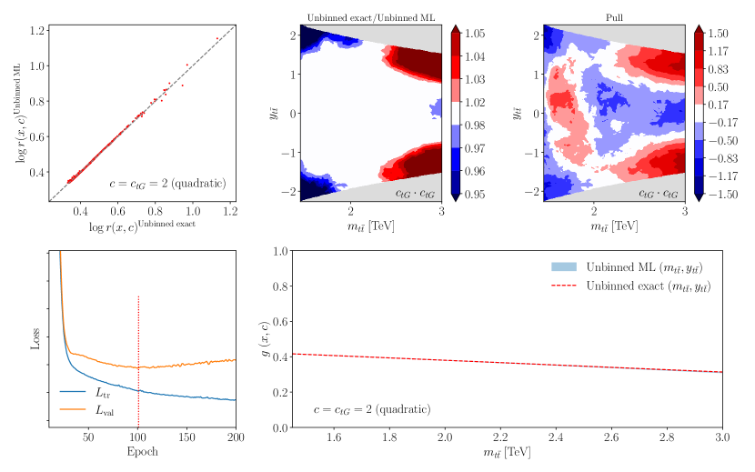
Figure 3.1: Validation of the machine learning parametrization of the EFT cross-section ratios when applied to the case of parton-level top quark pair production to be described in Sect. 4. The results shown here correspond to the training of the quadratic neural network $\mathrm{NN}^{(j,j)}(m_{t\bar{t}},y_{t\bar{t}})$ in Eq.(3.19) with $j$ indicating the chromomagnetic operator $c_{tG}$. From left to right and top to bottom we display a point-by-point comparison of the log-likelihood ratio in the ML model and the corresponding analytical calculation; the median of the ratio between the ML model and the analytical calculation and the associated pull in the $(m_{t\bar{t}},y_{t\bar{t}})$ feature space; the evolution of the loss function split in training and validation sets for a representative replica as a function of the number of training epochs; and the resultant decision boundary $g(\bm{x,c})$ for $c_{tG}=2$ including MC replica uncertainties at the end of the training procedure.

First, we display a point-by-point comparison of the log-likelihood ratio in the ML model and the corresponding analytical calculation, namely comparing Eqns. (3.19) and (3.7) evaluated on the kinematics of the Monte Carlo events generated for the training in the specific case of $c_{tG}=2$. One obtains excellent agreement within the full phase space considered. Then we show the median value (over replicas) of the ratio between the analytical and machine learning calculations of $\mathrm{NN}^{(j,j)}$ evaluated in the $\left(m_{t\bar{t}},y_{t\bar{t}}\right)$ kinematic feature space, with $j$ again being the chromomagnetic operator $c_{tG}$. We also show the pull between the analytical and numerical calculations in units of the Monte Carlo replica uncertainty. From the median plot we see that the parametrized ratio $\hat{r}_{\sigma}$ reproduces the exact result within a few percent except for low-statistics regions (large $|y_{t\bar{t}}|$ and $m_{t\bar{t}},y_{t\bar{t}}$ tails), and that these differences are in general well contained within the one-sigma MC replica uncertainty band.

The bottom right plot of Fig. 3.1 displays the resultant decision boundary $g(\bm{x,c})$ for $y_{t\bar{t}}=0$ as a function of the invariant mass $m_{t\bar{t}}$ in the training of the quadratic cross-section ratio proportional to $c_{tG}^{2}$ in the specific case of also for $c_{tG}=2$. The band in the ML model is evaluated as the 68% CL interval over the trained MC replicas, and is the largest at high $m_{t\bar{t}}$ values where statistics are the smallest. Again we find that the ML parametrization is in agreement within uncertainties when compared to the exact analytical calculation, further validating the procedure. Similar good agreement is observed for other EFT operators both for the linear and for the quadratic cross-sections.

4 Theoretical modeling

We describe here the settings adopted for the theoretical modeling and simulation of unbinned observables at the LHC and their subsequent SMEFT interpretation. We consider two representative processes relevant for global EFT fits, namely top-quark pair production and Higgs boson production in association with a $Z$-boson. We describe the calculational setups used for the SM and EFT cross-sections at both the parton and the particle level, justify the choice of EFT operator basis, motivate the selection and acceptance cuts applied to final-state particles, present the validation of our numerical simulations with analytical calculations whenever possible, and summarize the inputs to the neural network training.

4.1 Benchmark processes and simulation pipeline

We apply the methodology developed in Sect. 3 to construct unbinned observables for inclusive top-quark pair production and Higgs boson production in association with a $Z$-boson in proton-proton collisions. We evaluate theoretical predictions in the SM and in the SMEFT for both processes at leading order (LO), which suffices in this context given that we are considering pseudo-data. For particle-level event generation we consider the fully leptonic decay channel of top quark pair production,

$${\rm p}+{\rm p}\to t+\bar{t}\to b+\ell^{+}+\nu_{\ell}+\bar{b}+\ell^{-}+\bar{\nu}_{\ell}\,,$$ (4.1)

and that of the Higgs decaying to a pair of bottom quarks and with the $Z$-boson decaying leptonically,

$${\rm p}+{\rm p}\to h+Z\to b+\bar{b}+\ell^{+}+\ell^{-}\,.$$ (4.2)

The evaluation of the SM and SMEFT cross-sections at LO is carried out with MadGraph5_aMC@NLO [71] interfaced to SMEFTsim [72, 73] with NNPDF31_nnlo_as_0118 as the input PDF set [74]. As discussed in Sect. 3.2, at the quadratic level in the EFT we parametrize the cross-section ratio such that we have separate neural networks for terms proportional to $c_{j}^{2}$ and for the quadratic mixed terms $c_{j}c_{k}$  . In addition to Eq. (4.1), we also carry out $t\bar{t}$ simulations at the undecayed parton level with the goal of comparing with the corresponding exact analytical calculation of the likelihood ratio for benchmarking purposes. Such analytical evaluation becomes more difficult (or impossible) for realistic unbinned multivariate measurements presented in terms of particle-level or detector-level observables.

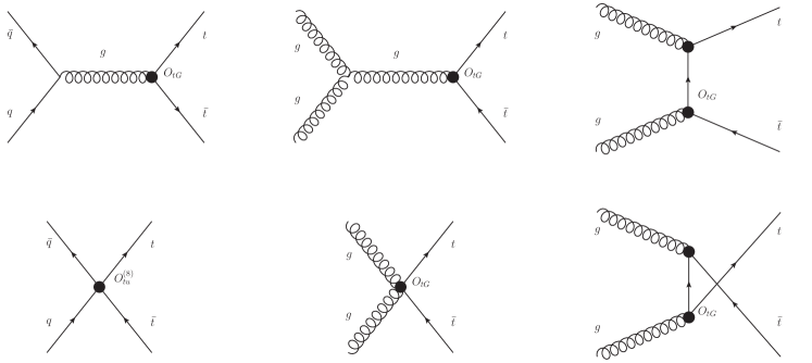
Figure 4.1: Representative Feynman diagrams for parton-level top-quark pair production in the SMEFT, indicating some of the corrections induced by the $O_{tG}$ and $O_{tu}^{(8)}$ operators. These operators both modify existing SM interaction vertices, such as $gt\bar{t}$, and induce new ones, such as $ggt\bar{t}$. The operators considered do not modify top quark decays.

smeftsim_main.fr

SMEFTsim Flavor = topU3l, Scheme=MwScheme

FeynArts .mod file

FeynArts .gen file

FeynArts: draw topologies and insert fields FormCalc: compute $\left|\mathcal{M}_{\mathrm{sm}}+\mathcal{M}_{\mathrm{eft}}(\bm{c})\right|^{2}$ Mathematica: compute $d\sigma(\bm{c})$ Analytical $d\sigma(\bm{c})$

Figure 4.2: Flow diagram displaying the pipeline adopted to evaluate at LO analytical expressions of differential distributions in the SMEFT for the LHC processes considered. These analytical cross-sections provide access to the exact likelihood ratio to benchmark the numerical MC simulations and the performance of the ML algorithm.

The flow chart in Fig. 4.2 describes the pipeline adopted to evaluate the analytical expressions for the parton level analysis at LO in the QCD expansion. First, we generate a FeynArts [75] model file from the SMEFTsim top U3l UFO model in the $\{m_{W},m_{Z},G_{F}\}$ input scheme [73]. This amounts to a $U(3)_{l}\times U(3)_{e}$ flavor symmetry in the leptonic sector and $U(2)_{q}\times U(3)_{d}\times U(2)_{d}$ in the quark sector, consistent with the flavor assumptions made in the SMEFiT analysis [15]. Then we use FeynArts to construct the diagrams associated to a given production process before passing pass them on to FormCalc_v9.9 [76] interfaced to Mathematica, that ultimately produces the analytical differential cross section in the SMEFT.

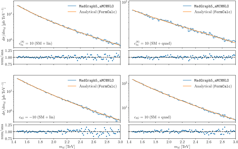
Figure 4.3: Parton level $m_{t\bar{t}}$ distribution in the analytical calculation of top-quark pair production at LO based on the pipeline of Fig. 4.2 compared with the corresponding numerical simulations based on MadGraph5_aMC@NLO. We display the SM predictions and those of the SMEFT for non-zero values of the $c_{tG}$ and $c_{tu}^{(8)}$ coefficients in the linear-only and quadratic-only cases. The bottom panels display the ratio between the numerical and analytical calculations.

Satisfactory agreement is found between the analytical SM and SMEFT calculations and the outcome of the corresponding MadGraph5_aMC@NLO simulations both at the linear and quadratic EFT level for all processes considered here. This agreement is illustrated by Fig. 4.3, comparing numerical and analytical SMEFT predictions for the $m_{t\bar{t}}$ distribution in top-quark pair production for some of the values of the $c_{tG}$ and $c_{tu}^{(8)}$ coefficients used for the neural network training. Similar agreement is found for other distributions and other points in the EFT parameter space. These analytical calculations also make possible validating the accuracy of the neural network training, as exemplified in Fig. 3.1, and indeed the agreement persists at the level of the training of the decision boundary $g(\bm{x},\bm{c})$.

Dominance of statistical uncertainties

As discussed in Sect. 2, we restrict our analysis to measurements dominated by statistical uncertainties for which correlated systematic uncertainties can be neglected. This condition can be enforced by restricting the fiducial phase space such that the number of events per bin satisfies

$${{\delta\sigma_{i}^{(\rm stat)}}\over{\sigma_{i}(\bm{0})}}={{1}\over{\sqrt{\nu_{i}(\bm{0})}}}\geq\delta_{\rm min}^{(\rm stat)}\,,\qquad i=1,\ldots,N_{b}\,,$$ (4.3)

where $\nu_{i}(\bm{0})$ is the number of expected events in bin $i$ according to the SM hypothesis after applying selection, acceptance, and efficiency cuts. The threshold parameter $\delta_{\rm min}^{(\rm stat)}$ is set to $\delta_{\rm min}^{(\rm stat)}=0.02$ for our baseline analysis. We have verified that our qualitative findings are not modified upon moderate variations of its value. Since Eq. (4.3) must apply for all possible binning choices, it should also hold for $N_{b}=1$, namely for the total fiducial cross-section. Therefore, we require that the selection and acceptance cuts applied lead to a fiducial region satisfying $(\delta\sigma_{\rm fid}^{(\rm stat)}/\sigma_{\rm fid})\geq\delta_{\rm min}^{(\rm stat)}$. This condition implies that the requirement of Eq. (4.3) will also be satisfied for any particular choice of binning, including the narrow bin limit, i.e. the unbinned case.

Within our approach there are two options by which the condition Eq. (4.3) can be enforced when applied to the fiducial cross-section, given by

$$\nu_{\rm tot}(\bm{0})=\mathcal{L}_{\rm int}\times\sigma_{\rm fid}(\bm{0})\,.$$ (4.4)

The first option is adjusting the integrated luminosity $\mathcal{L}_{\rm int}$ corresponding to this measurement. In this work we will take a fixed baseline luminosity $\mathcal{L}_{\rm int}=300$ fb^-1, corresponding to the integrated luminosity accumulated at the end of Run III. The second option is to adjust the fiducial region such that Eq. (4.3) is satisfied. Taking into account Eqns. (4.3) and (4.4), for a given luminosity $\mathcal{L}_{\rm int}$ the fiducial (SM) cross-section should satisfy

$$\sigma_{\rm fid}(\bm{0})\geq\left[\left(\delta_{\rm min}^{(\rm stat)}\right)^{2}\mathcal{L}_{\rm int}\right]^{-1}\,.$$ (4.5)

In this work we take the second option, imposing kinematic cuts restricting the events to the high-energy, low-yield tails of distributions, such as by means of a strong $m_{t\bar{t}}$ cut in the case of top quark pair production, see Table 4.2. It is then possible to generalize the results presented in this work for $\mathcal{L}_{\rm int}=300$ fb^-1 to higher integrated luminosities by making the cuts that define the fiducial region more stringent.

4.2 Top-quark pair production: parton level

For inclusive top quark pair production with stable tops the MadGraph5_aMC@NLO calculation is accompanied by and benchmarked against the analytical evaluation of the likelihood, see also Fig. 4.3. We consider the effects of two representative dimension-six SMEFT operators modifying inclusive top quark pair production, namely the chromomagnetic dipole operator $\mathcal{O}_{tG}$ and the two-light-two-heavy four-fermion color-octet operator $\mathcal{O}_{tu}^{(8)}$ defined as in [73] in the topU3l flavor scheme:

$$\mathcal{O}_{tu}^{(8)} =(\bar{t}\gamma_{\mu}T^{A}t)(\bar{u}\gamma^{\mu}T^{A}u)\,,$$

$$\mathcal{O}_{tG} =(\bar{Q}\sigma^{\mu\nu}T^{a}t)\tilde{H}G_{\mu\nu}^{a}\,.$$ (4.6)

Representative Feynman diagrams displaying SMEFT corrections associated to these operators in top-quark pair production are shown in Figs. 4.1. The dipole operator $\mathcal{O}_{tG}$ modifies the $gt\bar{t}$ coupling as well as induces new four-body $ggt\bar{t}$ interactions, while the four-fermion octet operator $\mathcal{O}_{tu}^{(8)}$ leads to a new $\bar{q}q\bar{t}t$ vertex.

At the level of undecayed tops, a $2\rightarrow 2$ process such as top quark pair production is uniquely determined by specifying three independent kinematic variables, since the four-momenta $p_{t}^{\mu}$ and $p_{\bar{t}}^{\mu}$ satisfy the mass-shell conditions and transverse momentum conservation. We refer to these kinematic variables as features in the context of ML classification problems. We choose the three independent features to be the transverse momentum of the top quark, $p_{T}^{t}$, and the invariant mass and rapidity of the top quark pair, $m_{t\bar{t}}$ and $y_{t\bar{t}}$ respectively. It can be verified how considering additional variables does not improve the sensitivity to the EFT parameters given the redundancy of the extra features. No fiducial cuts are imposed in the MadGraph5_aMC@NLO calculation to facilitate the comparison with the analytical result.

Concerning the event generation settings, for each point in the EFT parameter space ${\bm{c}}$ that enters the neural network training we generate $N_{\rm rep}=50$ independent sets of events (replicas) containing $\widetilde{N}_{\rm ev}=10^{5}$ events each, for a total of $5\times 10^{6}$ events, see also the overview in Table 4.5. Note that we adopt the convention whereby $\widetilde{N}_{\rm ev}$ denotes Monte Carlo events generated to train the machine learning classifier while $N_{\rm ev}=\nu_{\rm tot}$ indicates the physical events that enter the EFT parameter inference. The former can be made as large as one wants, while the latter is fixed by the assumed integrated luminosity and the value of the fiducial cross-section, Eq. (4.4). In addition, for each replica we generate an independent set of $10^{5}$ SM events. This is required so that the two terms of the cross-entropy loss function Eq. (3.9) are properly balanced, and results in a training set of $2\times 10^{5}$ events per replica. Similar settings are used by the particle level processes described next, and we have verified that the size of this Monte Carlo dataset is sufficient to ensure a stable and accurate parametrization of the likelihood ratio.

4.3 Top-quark pair production: particle level

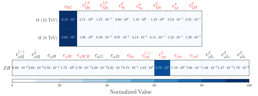
Figure 4.4: The diagonal entries of the Fisher matrix corresponding to the operators that enter the calculation of the LHC $t\bar{t}$ production at 8 TeV and 13 TeV (top) and of the $hZ$ production at 13 TeV (bottom) [15], where each row is normalized to 100. The dark blue entry indicates the operator that dominates the Fisher information, and those marked in red are selected to construct the unbinned observables.

In the particle-level case, where the top-quark events generated from the diagrams in Fig. 4.1 are decayed into the $b\ell^{+}\nu_{\ell}\bar{b}\ell^{-}\bar{\nu}_{\ell}$ final state, one considers a broader set of kinematic features. As in the parton level case, SM and EFT events are simulated with MadGraph5_aMC@NLO at LO in the QCD expansion, though now the analytical calculation is not available as a cross-check. In order to select the relevant EFT operators, we adopt the following strategy. Since we consider a single process, it is only possible to constrain a subset of operators, which are taken to be the $n_{\rm eft}$ Wilson coefficients with the highest Fisher information value, namely those that can be better determined from the fit. In the upper part of Fig. 4.4 we display the diagonal entries of the Fisher information matrix corresponding to the operators that enter the calculation of the LHC $t\bar{t}$ production measurements at 8 TeV and 13 TeV from [15], where each row is normalized to 100. The dark blue entry indicates the dominating operator, while the operators listed in red are those with the highest Fisher information and selected to construct the unbinned observables. Constraining additional Wilson coefficients would require extending the analysis to consider unbinned observables for processes such as $t\bar{t}V$ which span complementary directions in the parameter space.

In Table 4.1 we indicate the SMEFT operators entering inclusive top-quark pair production and listed in Fig. 4.4. For each operator we provide its definition in terms of the SM fields and the notation used to refer to the corresponding Wilson coefficients in SMEFTsim (in the topU3l flavor scheme), SMEFiT, and SMEFT@NLO [58]. These operator definitions are consistent with those used in the SMEFiT global analyses [77, 15] as required for the eventual integration of the unbinned observables there.

operator	SMEFiT	SMEFTsim	SMEFT@NLO	Definition
$\mathcal{O}_{tG}$	ctG	$-\verb|ctGRe|/\verb|gs|$	ctG	$ig_{s}(\bar{Q}\tau^{\mu\nu}T_{A}t)\tilde{\varphi}G_{\mu\nu}^{A}+\mathrm{h.c.}$
$\mathcal{O}_{Qq}^{1,8}$	c81qq	cQj18	cQq18	$\sum\limits_{i=1,2}c_{qq}^{1(i33i)}+3c_{qq}^{3(i33i)}$
$\mathcal{O}_{Qq}^{3,8}$	c83qq	cQj38	cQq38	$\sum\limits_{i=1,2}c_{qq}^{1(i33i)}-c_{qq}^{3(i33i)}$
$\mathcal{O}_{tq}^{8}$	c8qt	ctj8	ctq8	$\sum\limits_{i=1,2}c_{qu}^{8(ii33)}$
$\mathcal{O}_{tu}^{8}$	c8ut	ctu8	ctu8	$\sum\limits_{i=1,2}2c_{uu}^{(i33i)}$
$\mathcal{O}_{Qu}^{8}$	c8qu	cQu8	cQu8	$\sum\limits_{i=1,2}c_{qu}^{8(33ii)}$
$\mathcal{O}_{td}^{8}$	c8dt	ctd8 = ctb8	ctd8	$\sum\limits_{j=1,2,3}c_{ud}^{8(33jj)}$
$\mathcal{O}_{Qd}^{8}$	c8qd	cQd8 = cQb8	cQd8	$\sum\limits_{j=1,2,3}c_{qd}^{8(33jj)}$

Table 4.1: The SMEFT operators entering inclusive top-quark pair production. We indicate their definition in terms of the SM fields and the notation used for corresponding Wilson coefficients in SMEFTsim (in the topU3l flavor scheme), SMEFiT, and SMEFT@NLO. The = sign indicates that two coefficients are fixed to the same value [73].

kinematic feature	cut
$m_{t\bar{t}}$	$>1.45$ TeV
$p_{T}^{\ell}\>\rm{\leavevmode\nobreak\ (leading)}$	$>25$ GeV
$p_{T}^{\ell}\>\rm{\leavevmode\nobreak\ (trailing)}$	$>20$ GeV
$p_{T}^{j}$	$>30$ GeV
$|\eta^{j}|$	$<2.5$
$m_{\ell\bar{\ell}}$	$m_{\ell\bar{\ell}}>106$ GeV, or $m_{\ell\bar{\ell}}<76$ GeV and $m_{\ell\bar{\ell}}>20$ GeV
$\Delta R(j,\ell)$	$>0.4$
$p_{T}^{\rm{miss}}$	$>40$ GeV

Table 4.2: Selection and acceptance cuts imposed on the final-state particles of the $t\bar{t}\to b\bar{b}\ell^{+}\ell^{-}\nu_{\ell}\bar{\nu}_{\ell}$ process.

The selection and acceptance cuts imposed on the final-state particles of the $t\bar{t}\to b\bar{b}\ell^{+}\ell^{-}\nu_{\ell}\bar{\nu}_{\ell}$ process are adapted from the Run II dilepton CMS analysis [78] and listed in Table 4.2. Concerning the array of kinematic features ${\bm{x}}$, it is composed of $n_{k}=18$ features: $p_{T}$ of the lepton $p_{T}^{\ell}$, $p_{T}$ of the antilepton $p_{T}^{\bar{\ell}}$, leading $p_{T}^{\ell}$, trailing $p_{T}^{\ell}$, lepton pseudorapidity $\eta_{\ell}$, antilepton pseudorapidity $\eta_{\bar{\ell}}$, leading $\eta_{\ell}$, trailing $\eta_{\ell}$, $p_{T}$ of the dilepton system $p_{T}^{\ell\bar{\ell}}$, invariant mass of the dilepton system $m_{\ell\bar{\ell}}$, absolute difference in azimuthal angle $|\Delta\phi(\ell,\bar{\ell})|$, difference in absolute rapidity $\Delta\eta(\ell,\bar{\ell})$, leading $p_{T}$ of the $b$-jet, trailing $p_{T}$ of the $b$-jet, pseudorapidity of the leading $b$-jet $\eta_{b}$, pseudorapidity of the trailing $b$-jet $\eta_{b}$, $p_{T}$ of the $b\bar{b}$ system $p_{T}^{b\bar{b}}$, and invariant mass of the $b\bar{b}$ system $m_{b\bar{b}}$. These features are partially correlated among them, and hence maximal sensitivity of the unbinned observables to constrain the EFT coefficients will be achieved for $n_{k}<18$.

Since no parton shower or hadronization effects are included, the $b$-quarks can be reconstructed without the need of jet clustering and assuming perfect tagging efficiency. These simulation settings are not suited to describe actual data but suffice for the present analysis based on pseudo-data, whose goal is the consistent comparison of the impact on the EFT parameter space of unbinned multivariate ML observables with their binned counterparts.

4.4 Higgs associated production with a $Z$-boson

The second process that we consider is Higgs production in association with a $Z$-boson in the $b\bar{b}\ell^{+}\ell^{-}$ final state, for which representative Feynman diagrams indicating the impact of the EFT operators considered are displayed in Fig. 4.5. Following the same strategy as for top quark pair production, the bottom panel of Fig. 4.4 indicates in red the selected $n_{\rm eft}=7$ operators with the largest value of the Fisher information matrix when evaluated on the 13 TeV LHC $hZ$ production data. The definition of these operators, again consistent with those in [15], is listed in Table 4.3 and includes the bottom Yukawa coupling $\mathcal{O}_{b\varphi}$, purely bosonic operators such as $\mathcal{O}_{\varphi W}$ and $\mathcal{O}_{\varphi WB}$, and operators modifying the couplings between quarks and vector bosons such as $\mathcal{O}_{\varphi u}$ and $\mathcal{O}_{\varphi d}$.

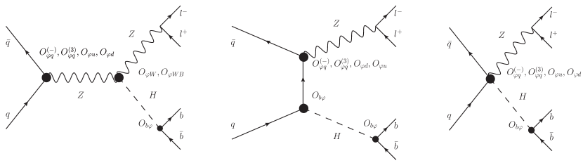
Figure 4.5: Same as Fig. 4.1 for Higgs associated production with a $Z$-boson, $hZ\to b\bar{b}\ell^{+}\ell^{-}$, indicating representative corrections arising from the SMEFT operators considered. For this process SMEFT effects modify also particle decays, in particular via the Yukawa interaction relevant for $h\to b\bar{b}$.

operator	SMEFTsim	SMEFiT	Definition
$\mathcal{O}_{\varphi u}$	cHu	cpui	$\sum_{i=1,2}(\varphi^{\dagger}iD_{\mu}\varphi)(\bar{u}_{i}\gamma^{\mu}u_{i})$
$\mathcal{O}_{\varphi d}$	cHd	cpdi	$\sum_{i=1,2}(\varphi^{\dagger}iD_{\mu}\varphi)(\bar{d}_{i}\gamma^{\mu}d_{i})$
$\mathcal{O}_{\varphi q}^{(1)}$	cHj1	$-$	$\sum_{i=1,2}i(\varphi^{\dagger}\overset{\text{\scriptsize$\leftrightarrow$}}{D}_{\mu}\varphi)(\bar{q}_{i}\gamma^{\mu}q_{i})$
$\mathcal{O}_{\varphi q}^{(3)}$	cHj3	c3pq	$\sum_{i=1,2}i(\varphi^{\dagger}\overset{\text{\scriptsize$\leftrightarrow$}}{D}_{\mu}\tau_{I}\varphi)(\bar{q}_{i}\gamma^{\mu}\tau^{I}q_{i})$
$\mathcal{O}_{\varphi q}^{(-)}$	cHj1 $-$ cHj3	cpqMi	$-$
$\mathcal{O}_{b\varphi}$	cbHRe	cbp	$(\varphi^{\dagger}\varphi)\bar{Q}b\varphi+\mathrm{h.c.}$
$\mathcal{O}_{\varphi W}$	cHW	cpW	$(\varphi^{\dagger}\varphi)W_{I}^{\mu\nu}W_{\mu\nu}^{I}$
$\mathcal{O}_{\varphi WB}$	cHWB	cpWB	$(\varphi^{\dagger}\tau_{I}\varphi)B^{\mu\nu}W^{I}_{\mu\nu}$

Table 4.3: Same as Table 4.1 for Higgs associated production in the $hZ\to b\bar{b}\ell^{+}\ell^{-}$ final state. Only the operators selected by the Fisher information analysis of Fig. 4.4 are displayed.

The selection and acceptance cuts imposed on the final-state particles of the $hZ\to b\bar{b}\ell^{+}\ell^{-}$ process are collected in Table 4.4 and have been adapted from the ATLAS Run II analysis [79]. In addition to these cuts, another cut on the jet cone radius $\Delta R$ in the $b\bar{b}$ system is applied depending on the value of $p_{T}^{Z}$, with $\Delta R(b_{1},b_{2})<3.0,1.8,1.2$ for $p_{T}^{Z}\in(75,150]$ GeV, $(150,200]$ GeV, and $(200,\infty)$ GeV respectively. The array of kinematic features ${\bm{x}}$ for this process is composed of the following $n_{k}=7$ features: the transverse momentum of the $Z$ boson $p_{T}^{Z}$, that of the $b$-quark $p_{T}^{b}$, that of the $b\bar{b}$ pair $p_{T}^{b\bar{b}}$, the angular separation $\Delta R_{b\bar{b}}$ of the $b$-quarks, their azimuthal angle separation $\Delta\phi_{b,b\bar{b}}$, the rapidity difference between the dilepton and the $b\bar{b}$ system $\Delta\eta_{Z,b\bar{b}}$, and the azimuthal angle separation $\Delta\phi_{\ell b}$. Again, most of these features are correlated among them and hence there will be a degree of redundancy in the analysis.

kinematic feature	cut
leading $b$-tagged jet $p^{b}_{T}$	$p^{b}_{T}>45$ GeV
$m_{b\bar{b}}$	$115<m_{b\bar{b}}<135$ GeV
$m_{\ell\bar{\ell}}$	$81<m_{\ell\bar{\ell}}<101$ GeV
$p_{T}^{\ell\bar{\ell}}$	$p_{T}^{\ell\bar{\ell}}>75$ GeV
$p_{T}^{\ell_{1}}$	$p_{T}^{\ell_{1}}>27$ GeV
$p_{T}^{\ell_{2}}$	$p_{T}^{\ell_{1}}>7$ GeV

Table 4.4: Selection and acceptance cuts imposed on the final-state particles of the $hZ\to b\bar{b}\ell^{+}\ell^{-}$ process.

4.5 Inputs to the neural network training

Fig. 4.6 displays the differential distributions in the kinematic features used to parametrize the likelihood ratio Eq. (3.19) in the $hZ\to b\bar{b}\ell^{+}\ell^{-}$ process. We compare the SM predictions with those obtained in the SMEFT when individual operators are activated for the values of the Wilson coefficients used for the neural network training. Results are shown separately at the linear-only and quadratic-only level, to highlight how in our approach the learning strategy separates the training of the linear from the quadratic cross-section ratios, see also Sect. 3.2. In order to illustrate shape (rather than normalization) differences of the NN inputs, all distributions are normalized by their fiducial cross-sections. The corresponding comparisons at the level of the $t\bar{t}\to b\bar{b}\ell^{+}\ell^{-}\nu_{\ell}\bar{\nu}_{\ell}$ process, displaying the complete set of $n_{k}=18$ kinematic features used to train the cross-section ratio at the quadratic-only level, are shown in Fig. 4.7.

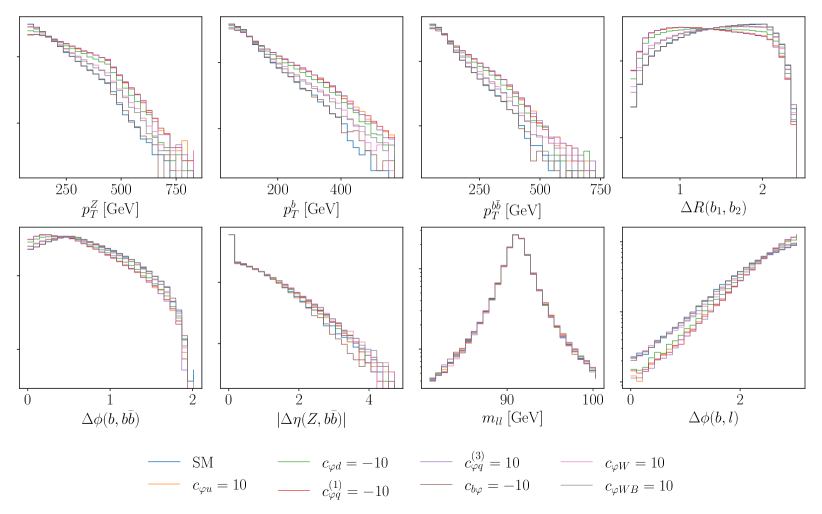
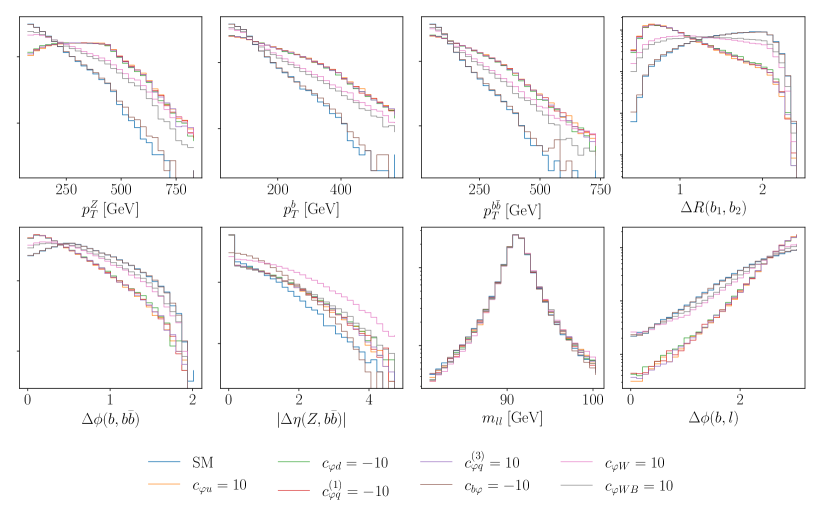
Figure 4.6: Differential distributions in the kinematic features used to parametrize the likelihood ratio in the $hZ\to b\bar{b}\ell^{+}\ell^{-}$ process. We compare the SM predictions with those obtained in the SMEFT when individual operators are activated for coefficient values used for the neural network training. Results are shown separately at the linear-only level (upper) and quadratic-only (bottom panels) level and normalized to their fiducial cross-sections.

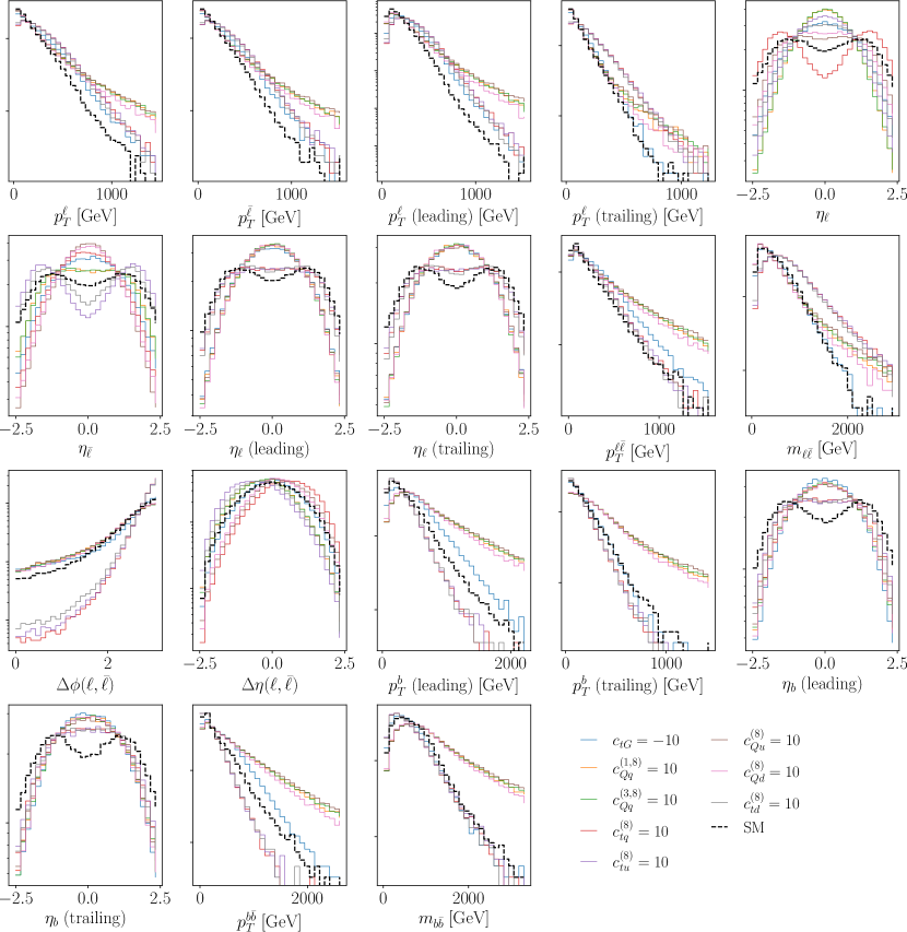
Figure 4.7: Same as the bottom panels in Fig. 4.6 (quadratic-only EFT effects included) for the $n_{k}=18$ kinematic features entering the parametrization of the likelihood ratio in the $t\bar{t}\to b\bar{b}\ell^{+}\ell^{-}\nu_{\ell}\bar{\nu}_{\ell}$ process.

From Figs. 4.6 and 4.7 one can observe how each operator modifies the qualitative shape of the various kinematic features in different ways. Furthermore, in general the EFT quadratic-only corrections enhance the shift with respect to the SM distributions as compared to the linear ones. The complementarity of the information provided by each kinematic feature motivates the inclusion of as many final-state variables as possible when constructing unbinned observables, though as mentioned above the limiting sensitivity will typically be saturated before reaching the total number of kinematic features used for the training.

As mentioned in Sect. 3.3, an efficient neural network training strategy demands that the kinematic features $\bm{x}$ entering the evaluation of the $r_{\sigma}(\bm{x},\bm{c})$ cross-section ratios are preprocessed to ensure that the input information is provided to the neural networks in the region of maximal sensitivity. That is, all features should be transformed to a common range and their distribution within this range should be reasonably similar. Here we use a robust scaler to ensure that this condition is satisfied. Fig. 4.8 displays the comparison between two different preprocessing schemes applied to the input features before the neural network training of the $hZ\to b\bar{b}\ell^{+}\ell^{-}$ likelihood is carried out. We display results for a Standardized Gaussian scaler and for a robust scaler: the latter subtracts the median and scales to the $95\%$ inter-quantile range, while the former rescales all features to have zero mean and unit variance. The robust scaler leads to input feature distributions peaked around zero with their bulk contained within the $[-1,1]$ region, which is not the case in general for the Standardized Gaussian scaler. Therefore our default robust scaler facilitates the incorporation of new kinematic features, since the shapes of the input distributions are such that their bulk belongs to the high-sensitivity region of the neural networks.

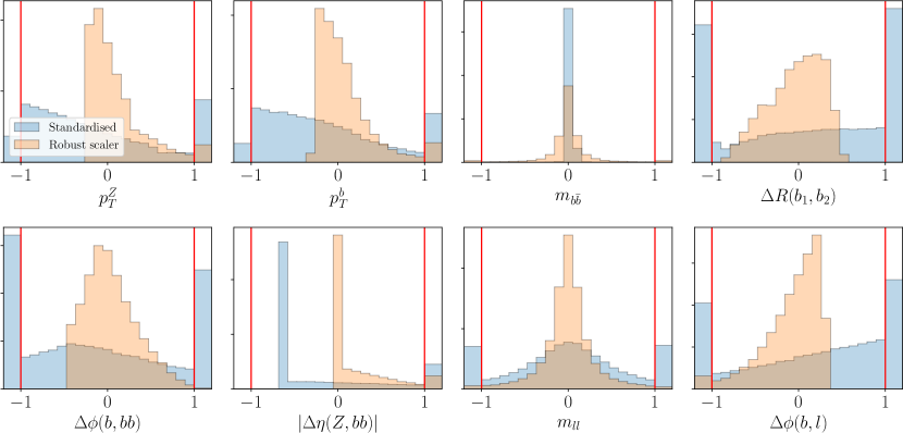
Figure 4.8: Comparison between two different data preprocessing schemes applied to the input features in the neural network training of the $hZ\to b\bar{b}\ell^{+}\ell^{-}$ likelihood: a Standardized Gaussian scaler and a robust scaler adopting a $95\%$ inter-quantile range.

Table 4.5 summarizes the settings adopted for the neural network training of the likelihood ratio function Eq. (3.19) for the processes considered. For each process, we indicate the number of replicas $N_{\rm rep}$ generated, the values of the EFT coefficients that enter the training as specified in Eqns. (3.12) and (3.15), the number of Monte Carlo events generated $\widetilde{N}_{\rm ev}$ for each replica, and the number of neural networks to be trained per replica $N_{\rm nn}$. The values of the Wilson coefficients are chosen to be sufficiently large so as to mitigate the effect of MC errors that might otherwise dominate the SM-EFT discrepancy. Furthermore, the sign of each Wilson coefficient is chosen such that the effect of the EFT is an enhancement relative to the SM, and therefore the differential cross sections are consistently positive. For example, in the case of negative EFT-SM interference, we select negative values of Wilson coefficients. Cross-section positivity must also be maintained during training of the neural networks, and this is further discussed in Sect. 3.2. The last column indicates the total number of trainings required to assemble the full parametrization including the $N_{\rm rep}$ replicas, namely $\#{\rm trainings}=N_{\rm rep}\times N_{\rm nn}$. For parton- and particle-level top-quark pair production and for $hZ$ production our procedure requires the training of 200, 1000, and 1500 networks respectively in the case of the quadratic EFT analysis. As discussed in Sect. 3 these trainings are parallelizable and the overall computational overhead remains moderate.

The values listed in the last two columns of Table 4.5 correspond to the case of quadratic EFT fits, since as will be explained in Sect. 5 at the linear level the presence of degenerate directions requires restricting the subset of operators for which inference can be performed. For each process, the total number of Monte Carlo events in the SMEFT that need to be generated is therefore $\widetilde{N}_{\rm ev}\times N_{\rm rep}\times N_{\rm nn}$, and in addition the training needs a balanced SM sample composed by $\widetilde{N}_{\rm ev}\times N_{\rm rep}$ events. For example, in the case of $hZ$ production the total number of SMEFT events to be generated is $10^{5}\times 50\times 30=1.5\times 10^{8}$ events.

Process	$\quad N_{\rm rep}\quad$	$c_{j}^{(\rm tr)}$	$\widetilde{N}_{\rm ev}$ (per replica)	$\quad N_{\rm nn}\quad$	#trainings
$pp\to t\bar{t}$	50	$c_{tG}=-10$ $c_{tu}^{(8)}=10$	$10^{5}$	4	200
$pp\to t\bar{t}\to b\bar{b}\ell^{+}\ell^{-}\nu_{\ell}\bar{\nu}_{\ell}$	25	$c_{td}^{(8)}=10$ $c_{Qd}^{(8)}=10$ $c_{Qq}^{(1,8)}=10$ $c_{Qq}^{(3,8)}=10$ $c_{Qu}^{(8)}=10$ $c_{tG}=-10$ $c_{qt}^{(8)}=10$ $c_{tu}^{(8)}=10$	$10^{5}$	$40$	1000
$pp\to hZ\to b\bar{b}\ell^{+}\ell^{-}$	50	$c_{\varphi u}=10$ $c_{\varphi d}=-10$ $c_{\varphi q}^{(1)}=-10$ $c_{\varphi q}^{(3)}=10$ $c_{b\varphi}=-10$ $c_{\varphi W}=10$ $c_{\varphi WB}=10$	$10^{5}$	$30$	1500

Table 4.5: Overview of the settings for the neural network training of the likelihood ratio Eq. (3.19). For each process, we indicate the number of replicas $N_{\rm rep}$, the values of the EFT coefficients that enter the training as specified in Eqns. (3.12) and (3.15), the number of Monte Carlo events generated $\widetilde{N}_{\rm ev}$ for each replica, and the number of neural networks to be trained per replica $N_{\rm nn}$ taking into account that some EFT cross-sections vanish at the linear level. The values of the Wilson coefficients are chosen such that the EFT has a large effect relative to the SM, mitigating the effect of MC errors that could otherwise dominate the SM-EFT discrepancy. The signs of the Wilson coefficients are chosen such that the EFT always leads to an enhancement relative to the SM; for example, negative Wilson coefficients are chosen to compensate for negative SM-EFT interference. This ensures positive differential cross-sections throughout the training samples. The last column indicates the total number of trainings required, $\#{\rm trainings}=N_{\rm rep}\times N_{\rm nn}$. The last two columns correspond to the case of quadratic EFT fits; at the linear EFT level the presence of quasi-flat directions restricts the subset of operators for which inference can be performed. For each process, the total number of Monte Carlo EFT events generated is $\widetilde{N}_{\rm ev}\times N_{\rm rep}\times N_{\rm nn}$, and in addition we need balanced SM samples requiring $\widetilde{N}_{\rm ev}\times N_{\rm rep}$ events.

5 EFT constraints from unbinned multivariate observables

We now present the constraints on the EFT parameter space provided by the unbinned observables constructed in Sect. 3 in comparison with those provided by their binned counterparts. We study the dependence of these results on the choice of binning and on the kinematic features. We also quantify how much the EFT constraints are modified when restricting the analysis to linear $\mathcal{O}(\Lambda^{-2})$ effects as compared to when the quadratic $\mathcal{O}(\Lambda^{-4})$ contributions are also included.

First, we describe the method adopted to infer the posterior distributions of the EFT parameters for a given observable, either binned or unbinned. Second, we present results for parton-level inclusive top quark pair production, described in Sect. 4.2. The motivation for this is to validate our machine learning methodology by comparing it with the results of parameter inference based on the analytical calculation of the likelihood. Then we consider the analogous process, now at the particle level in the dilepton final state (Sect. 4.3), and quantify the information gain resulting from unbinned observables and its dependence on the choice of kinematic features used in the training. This is followed by the corresponding analysis for $hZ$ production (Sect. 4.4). Finally, we will discuss the impact of methodological uncertainties, discussed in Sect. 3.3, on the constraints we obtain on the EFT parameter space. The results presented here can be reproduced and extended to other processes by means of the ML4EFT framework, summarized in App. A.

5.1 EFT parameter inference

For each of the LHC processes considered in Sect. 4, Monte Carlo samples in the SM and the SMEFT are generated in order to train the decision boundary $g({\bm{x}},\bm{c})$ from the minimization of the cross-entropy loss function Eq. (3.8). See Tables 4.2 and 4.4 for the pseudodata generation settings. The outcome of the neural network training is a parametrization of the cross-section ratio $\hat{r}_{\sigma}(\bm{x},\bm{c})$, Eq. (3.19), which in the limit of large statistics and perfect training reproduces the true result $r_{\sigma}(\bm{x},\bm{c})$, Eq. (3.4). To account for finite-sample and finite network flexibility effects, we use the Monte Carlo replica method as described in Sect. 3.3 to estimate the associated methodological uncertainties. Therefore, the actual requirement that defines a satisfactory neural network parametrization $\hat{r}_{\sigma}$ is that it reproduces the exact result $r_{\sigma}$, within the 68% CL replica uncertainties evaluated from the ensemble Eq. (3.23).

From the exact result for the cross-section ratio $r_{\sigma}(\bm{x},\bm{c})$, or alternatively its ML representation $\hat{r}_{\sigma}(\bm{x},\bm{c})$, one can carry out inference on the EFT Wilson coefficients by means of the profile likelihood ratio Eq. (2.22) applied to the $N_{\rm ev}$ generated pseudo-data events. We emphasize that the $N_{\rm ev}$ events entering in Eq. (2.22), or alternatively in Eq. (3.6), are the physical events expected after acceptance and selection cuts for a given integrated luminosity $\mathcal{L}_{\rm int}$, see also the discussion in Sect. 4.1. The Monte Carlo events used to train the ML classifier are instead different: in general, the classifier is trained on a larger event sample than the one expected for the actual measurement. Once the machine learning parametrization of the cross-section ratio, Eq. (3.19), has been determined alongside its replica uncertainties, the profile likelihood ratio Eq. (2.22) can be used to infer the posterior probability distribution in the EFT parameter space and thus determine confidence level intervals associated to the unbinned observables. The same method is applied to binned likelihoods and eventually to extended likelihoods which combine the information provided by binned and unbinned observables, Eq. (2.24).

In this work, the EFT parameter inference based on the machine learning parametrization of the PLR is carried out by means of the Nested Sampling algorithm, in particular via the MultiNest implementation [80]. We recall that this is the baseline sampling algorithm used in the SMEFiT analysis [15] to determine the posterior distributions in the EFT parameter space composed of $n_{\rm eft}=36$ independent Wilson coefficients. The choice of MultiNest is motivated from its previous applications to EFT inference problems of comparable complexity to those relevant here, and also to facilitate the integration of unbinned observables into global EFT fits. The posterior distributions provided by MultiNest are represented by $N_{s}$ samples in the EFT parameter space, where $N_{s}$ is determined by requiring a given accuracy in the sampling procedure. From this finite set of samples, contours of the full posterior can be reconstructed via the kernel density estimator (KDE) method, also used e.g. in the context of Monte Carlo PDF fits [81, 82].

Methodological uncertainties associated to the $N_{\rm rep}$ replicas are propagated to the constraints on the EFT parameter space in two complementary ways. Firstly, after evaluating the neural networks on the $N_{\rm ev}$ events entering into the inference procedure, we calculate the median of each $\mathrm{NN}^{(j)}_{i}(\bm{x})$ and $\mathrm{NN}^{(j,k)}_{i}(\bm{x})$ in Eq. (3.23). The corresponding median profile likelihood ratio is then calculated and used in the Nested Sampling algorithm, from which contours of the posterior distribution are obtained. The results shown in the following Sects. 5.2, 5.3 and 5.4 have been produced using this method. Alternatively, one can assess the impact of the 2-$\sigma$ methodological uncertainties on these contours. We do so by defining $N_{\rm rep}$ profile likelihood ratios, one from each of the $N_{\rm rep}$ replicas, and performing Nested Sampling for each, resulting in $N_{\rm rep}$ sets of $N_{\rm s}$ samples from the EFT posterior distribution. The samples are then combined, and the KDE method used to determine contours of the posterior distribution. In Sect. 5.5 we will assess the differences observed between these two methodologies.

5.2 Top-quark pair production: parton level results

Fig. 5.1 displays the 95% CL contours in the $(c_{tG},c_{tu}^{(8)})$ plane obtained from the parton-level top quark pair production process described in Sect. 4.2. We compare the results based on EFT calculations at the linear level with those also including quadratic contributions. The black cross indicates the SM result, which is the hypothesis assumed in the generation of the pseudo-data that enters the inference procedure. The results shown here and in the remainder of this section correspond to a center-of-mass energy of $\sqrt{s}=14$ TeV and an integrated luminosity of $\mathcal{L}=300$ fb^-1. We show contours corresponding to two binned analyses, the first based on a coarse binning (Binning 1) in two kinematic features $m_{t\bar{t}}$ and $y_{t\bar{t}}$, defined by

$$m_{t\bar{t}}\in\left[1.45,2.5,\infty\right)\;\mathrm{TeV}\,,\quad y_{t\bar{t}}\in\pm\left[0,1.5,3.0\right]\,,$$

and the second based on a finer binning (Binning 2), given by

$$m_{t\bar{t}} \in \left[1.45,1.5,1.55,1.6,1.7,1.8,1.9,2.0,2.1,2.2,2.3,2.4,2.5,2.6,2.7,2.8,2.9,3.0,\infty\right)\;\mathrm{TeV}\,,$$

$$y_{t\bar{t}} \in \pm\left[0,0.3,0.6,0.9,1.2,3.0\right]\,.$$

Furthermore, we show results for the corresponding observable based on a single feature, the invariant mass $m_{t\bar{t}}$, obtained by marginalizing the double differential binning over the rapidity $y_{t\bar{t}}$. The contours derived from these two binned observables in Fig. 5.1 are compared with the corresponding unbinned observables constructed either with the analytic likelihood calculation (“Unbinned exact”) or with its machine learning parametrization (“Unbinned ML”).

For the two-feature observable in the quadratic case, upper right panel in Fig. 5.1, we observe how the 95% CL contours shrink first when moving from a coarser binning to a finer binning and then further when using the unbinned observable. Good agreement is found between the inference carried out with the exact likelihood calculation and with its ML interpolation, with the small remaining differences covered by the spread of the replicas as discussed below. We observe that the constraints on the chromomagnetic operator $c_{tG}$ are similar for the various observables considered, as expected, since it is mostly determined from the absolute normalization of the $t\bar{t}$ fiducial cross-section and hence adding kinematic information on the shape of the distributions does not provide significant extra information. The main improvement is seen in the constraints on the two-light-two-heavy operator $c_{tu}^{(8)}$, which benefits from exploiting the kinematic information.

By comparing with the corresponding analysis based on the single-feature $m_{t\bar{t}}$ observable (bottom right panel) one finds a moderate worsening of the obtained bounds. No major differences are observed, however, indicating how in this case the addition of $y_{t\bar{t}}$ as kinematic feature does not significantly modify the inference results. We have verified that good agreement is found between the exact likelihood calculation and the binned approach when a sufficiently fine binning is taken, as expected, because in the limit of infinitely fine bins the binned approach will exactly reproduce the analytical calculation. This is illustrated by Binning 3, given by

$$m_{t\bar{t}} \in \left[1.45,1.5,1.55,1.6,1.7,1.8,\dots,4.8,4.9,5.0,\infty\right)\;\mathrm{TeV}.$$

We have also verified that in this relatively simple scenario (a $2\to 2$ process) the addition of a third independent kinematic feature such as $p_{T}^{t}$ to the unbinned observable does not affect the outcome. As we show next, for a more realistic particle-level configuration it is instead clearly beneficial to increase the number of kinematic features considered in the EFT parameter inference.

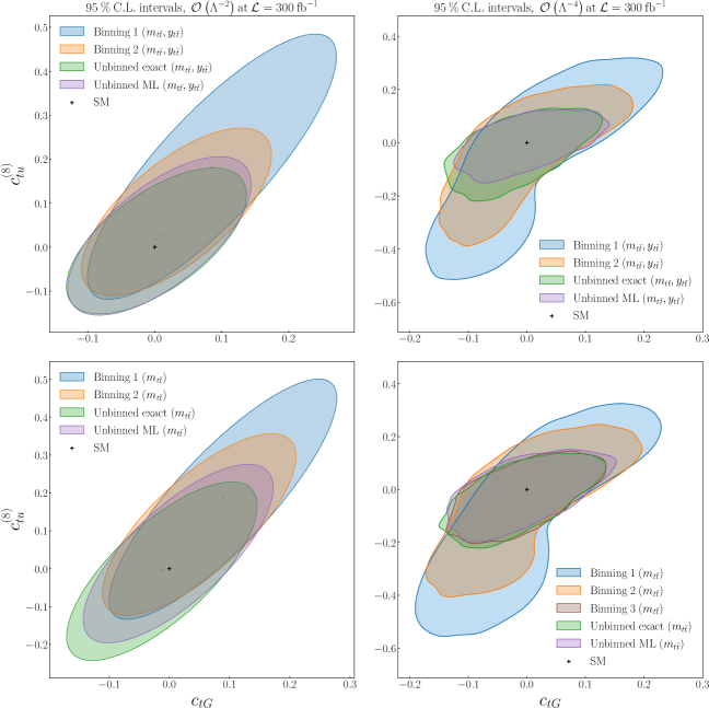
Figure 5.1: The 95% CL regions in the $(c_{tG},c_{tu}^{(8)})$ plane obtained for the parton-level top quark pair production process described in Sect. 4.2. We present results based on EFT calculations at the linear level (left) and also including quadratic contributions (right panels). The black cross indicates the SM result, which is the hypothesis assumed in the generation of the pseudo-data that enters the inference procedure. We compare the results from two binned analyses (Binning 1 and 2) with those of the corresponding unbinned observable, constructed either with the analytic likelihood calculation or with its machine learning parametrization. We demonstrate how the analytical calculation is reproduced for a sufficiently fine binning (Binning 3). We display the contours corresponding to two different observables, the first built upon two kinematic features $(m_{t\bar{t}},y_{t\bar{t}})$ (upper) and the second based on the invariant mass $m_{t\bar{t}}$ as a single feature (lower panels).

In the case of the linear EFT level results, displayed in left panels in Fig. 5.1, we note that there is a strong correlation between the two coefficients for the case of the coarse binning, indicating a quasi-flat direction. This is removed by using first a finer binning and then the unbinned observable, which in this case provides only a moderate improvement as compared to the finer binning. As in the case of the quadratic analysis, adding a second feature, $y_{t\bar{t}}$, does not significantly modify the results relative to the analysis of a single feature $m_{t\bar{t}}$.

5.3 Top-quark pair production: particle level results

We assess next the bounds on the EFT parameter space obtained from unbinned observables in the case of particle-level top quark pair production, specifically in the dilepton final state described in Sect. 4.3, $pp\to t\bar{t}\to b\ell^{+}\nu_{\ell}\bar{b}\ell^{-}\bar{\nu}_{\ell}$. As discussed there, this process is most sensitive to the $n_{\rm eft}=8$ operators with the highest Fisher information in inclusive $t\bar{t}$ production, as listed in Table 4.1. While for the quadratic EFT analysis it is possible to derive the posterior distribution associated to the full set of $n_{\rm eft}=8$ operators, at the linear level there are quasi-flat directions that destabilize the ML training of the likelihood ratio and the subsequent parameter inference. For this reason, in the linear EFT analysis of this process we consider a subset of $n_{\rm eft}=5$ operators that can be simultaneously constrained from inclusive top-quark pair production [83], given by

$$c_{tG},c_{qt}^{(8)},c_{Qu}^{(8)},c_{Qq}^{(1,8)},c_{td}^{(8)}\,.$$ (5.1)

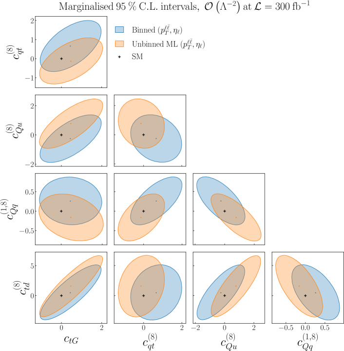
Figure 5.2: Pair-wise 95% CL contours for the Wilson coefficients entering top quark pair production in the dilepton final state, see Sect. 4.3 for more details. These contours are obtained by marginalizing over the full posterior distribution provided by Nested Sampling. We consider here $n_{\rm eft}=5$ Wilson coefficients that can be simultaneously constrained from inclusive top-quark pair production at the linear level in the EFT expansion. We compare the results obtained from both binned and unbinned ML observables constructed on the $(p_{T}^{\ell\bar{\ell}},\eta_{\ell})$ kinematic features. As in Fig. 5.1, the black cross indicates the SM values used to generate the pseudo-data that enters the inference. The comparison of the unbinned ML observable trained on $(p_{T}^{\ell\bar{\ell}},\eta_{\ell})$ with its counterpart trained on the full set of $n_{k}=18$ kinematic features is displayed in Fig. 5.3.

For this process we construct $n_{k}=18$ kinematic features built from the four-vectors of the final-state leptons and $b-$quarks. Considering further kinematic variables such as the missing $E_{T}$ would be redundant and not provide additional information. The distribution of these kinematic features in the SM and when quadratic EFT corrections are accounted for is displayed in Fig. 4.7, showing how different features provide complementary information to constrain the EFT and thus making a fully-fledged multivariate analysis both interesting and necessary in order to fully capture the EFT effects. For example, the pseudo-rapidity distributions bend around $\eta=0$ corresponding to the direction transverse to the beam pipe, while the transverse momenta are sensitive to energy growing effects in the high-$p_{T}$ tails of the distributions.

Fig. 5.2 displays the pair-wise 95% CL intervals for the $n_{\rm eft}=5$ Wilson coefficients in Eq. (5.1) relevant for the description of top quark pair production at the linear $\mathcal{O}(\Lambda^{-2})$ level. The black cross indicates the SM scenario used to generate the pseudo-data that enters the inference. The 95% CL contours shown are obtained from the full posterior distribution provided by Nested Sampling, marginalizing over the remaining Wilson coefficients for each of the operator pairs, with the ellipses drawn from the $N_{s}$ posterior samples provided by MultiNest. These are compared with the bounds provided by a binned observable based on the dilepton transverse momentum $p_{T}^{\ell\bar{\ell}}$ and the lepton pseudorapidity $\eta_{\ell}$ as kinematic features, where the binning is defined as

$$p_{T}^{\ell\bar{\ell}} \in \left[0,10,20,40,60,100,150,400,\infty\right)\,\textrm{GeV},$$

$$\eta^{\ell} \in \left[0,0.3,0.6,0.9,1.2,1.5,1.8,2.1,2.5\right]\,.$$

As for the parton-level case, a cut in the invariant mass $m_{t\bar{t}}$ is applied to ensure that Eq. (4.3) is satisfied and that statistical uncertainties dominate. Note that for all observables the pseudo-dataset used for the EFT parameter inference is the same and was not used during training.

From the comparisons in Fig. 5.2 one can observe how, for all observables and all operator pairings, the 95% CL intervals include the SM values used to generate the pseudo-data. The bounds obtained from the binned and unbinned observables are in general similar and compatible, and no major improvement is obtained with the adoption of the latter in this case. However, here we consider only $n_{k}=2$ kinematic features and hence ignore the potentially useful information contained in other variables that can be constructed from the final state kinematics. In order to assess their impact, Fig. 5.3 displays the same pair-wise marginalized comparison, now between ML unbinned observables with only $p_{T}^{\ell\bar{\ell}}$ and $\eta_{\ell}$ as input features and with the full set of $n_{k}=18$ kinematic variables displayed in Fig. 4.7. We now find a very significant change in the bounds on the EFT parameter space, improving by up to an order of magnitude or better in all cases. Again, the 95% CL contours include the SM hypothesis used to generate the pseudo-data. Furthermore, the inclusion of the full set of kinematic features reduces the correlations between operator pairs that arise when only $p_{T}^{\ell\bar{\ell}}$ and $\eta_{\ell}$ are considered, indicating a breaking of degeneracies in parameter space. This result indicates that a multivariate analysis improves the information on the EFT parameter space that can be extracted from this process as compared to that obtained from a subset of kinematic features.

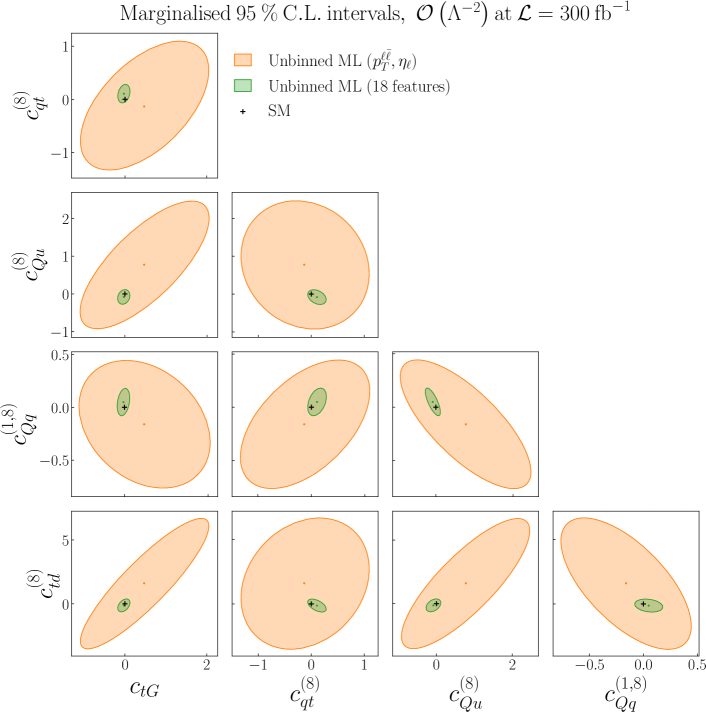
Figure 5.3: Same as Fig. 5.2 comparing the bounds on the EFT coefficients from the ML unbinned observables trained on $(p_{T}^{\ell\bar{\ell}},\eta_{\ell})$ and on the full set of $n_{k}=18$ kinematic features listed in Sect. 4.3, see also Fig. 4.7.

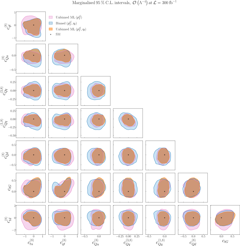
Figure 5.4: Same as Fig. 5.2 in the case of the EFT analysis carried out at the quadratic $\mathcal{O}(\Lambda^{-4})$ level. We display the results for pair-wise contours obtained from the marginalization of the posterior distribution in the space of $n_{\rm eft}=8$ Wilson coefficients. In comparison with the linear EFT analysis, it becomes possible to constrain three more coefficients from the same process once quadratic corrections are accounted for. We also include in this comparison the results obtained from the unbinned ML analysis based on $p_{T}^{\ell\bar{\ell}}$ as the single input feature.

We note that that the results displayed in Figs. 5.2 and 5.3 are expected to differ should the starting point be a global EFT analysis rather than a flat prior as is the case in the present proof-of-concept analysis. For instance, the two-light-two-heavy operators entering $t\bar{t}$ production at the linear level are highly correlated, which means that adopting a multivariate analysis leads to a sizable effect partly because it breaks degeneracies in the parameter space. Hence, the actual impact of unbinned multivariate observables for EFT analyses depends on which other datasets and processes are considered and can only be assessed on a case-by-case basis. In this respect, beyond the implications for the specific processes considered in this work, what our framework provides is a robust method to quantify the information on the EFT parameters provided by different types of observables constructed on exactly the same dataset: binned versus unbinned, different choices of binnings, and different numbers and types of kinematic features.

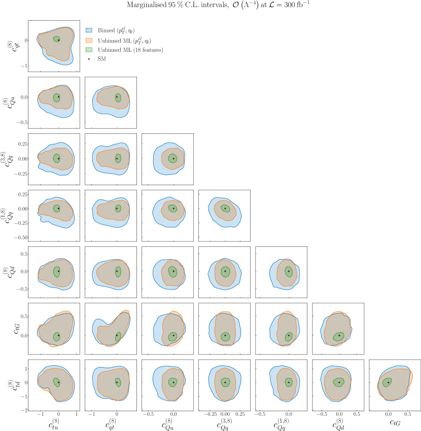
Figure 5.5: Same as Fig. 5.4 comparing the bounds obtained from the binned and unbinned observables built upon two kinematic features, $p_{T}^{\ell\bar{\ell}}$ and $\eta_{\ell}$, with the corresponding results for the unbinned ML observable trained on the full set of $n_{k}=18$ kinematic features.

As is well known, in top quark pair production quadratic EFT corrections are important for most operators, in particular due to energy-growing effects in the tails of distributions. These sizable effects are highlighted by the distortions with respect to the SM distributions induced by quadratic EFT effects, shown in Fig. 4.7, in the kinematic features used to train the ML classifier for this process. In order to investigate how the results based on linear EFT calculations vary once quadratic corrections are considered, in Figs. 5.4 and 5.5 we present the analogous comparisons to Figs. 5.2 and 5.3 respectively in the case of EFT calculations that also include the quadratic corrections. We display the results for pair-wise contours obtained from the marginalization of the posterior distribution in the space of the full set of $n_{\rm eft}=8$ Wilson coefficients, given that once quadratic corrections are accounted for it becomes possible to constrain the full set of relevant operators simultaneously. We also include in Fig. 5.4 the results obtained from the unbinned ML analysis based on $p_{T}^{\ell\bar{\ell}}$ as the single input feature, while Fig. 5.5 also displays the two-feature binned contours as reference. We note that once quadratic effects are accounted for the 95% CL contours will in general not be elliptic, and may even be composed of disjoint regions in the case of degenerate maxima.

Comparing the constraints provided by the binned $(p_{T}^{\ell\bar{\ell}},\eta_{\ell})$ observable in Fig. 5.4 with those in Figs. 5.2, one observes how the bounds on the EFT coefficients are improved when accounting for the quadratic EFT corrections. This improvement is consistent with the large quadratic corrections to the kinematic distributions entering the likelihood ratio of this process which lead to an enhanced sensitivity, and with previous studies [15, 77] within global SMEFT analyses. From the results Fig. 5.4 we find that for all operator pairs considered, the most stringent bounds are provided by the unbinned observable built upon the $(p_{T}^{\ell\bar{\ell}},\eta_{\ell})$ pair of kinematic features. Furthermore, one can identify the factor which brings in more information: either using the full event-by-event kinematics for a given set of features, or increasing the number of kinematic features being considered. For some operator combinations, the dominant effect turns out to be that of adding a second kinematic feature, for instance in the case of $(c_{tu}^{(8)},c_{td}^{(8)})$ binned and unbinned observables coincide when using the $(p_{T}^{\ell\bar{\ell}},\eta_{\ell})$ features while the unbinned $p_{T}^{\ell\bar{\ell}}$ observable results in larger uncertainties. For other cases, it is instead the information provided by the event-by-event kinematics which dominates, for example in the $(c_{Qq}^{(3,8)},c_{Qu}^{(8)})$ plane the constraints from binned $(p_{T}^{\ell\bar{\ell}},\eta_{\ell})$ are clearly looser than those from their unbinned counterparts.

The comparison between the constraints on the EFT parameter space provided by the unbinned observable based on two kinematic features, $(p_{T}^{\ell\bar{\ell}},\eta_{\ell})$, and those provided by its counterpart based on the full set $n_{k}=18$ kinematic features is displayed in Fig. 5.5. It confirms that at the quadratic level there is also a marked gain in constraining power obtained from increasing the number of kinematic variables considered in the analysis. For reference, the plot also displays the bounds obtained with the two-feature binned observable in the same process. Interestingly, when considering the full set of kinematic features, one obtains posterior contours which display a reduced operator correlation, highlighting how the unbinned multivariate operator is especially effective at removing (quasi)-degeneracies in the EFT coefficients. As for the linear case, the improvement in the bounds obtained with the multivariate can reach up to an order of magnitude as compared to the two-feature unbinned analysis.

One can compare the bounds obtained in the present study with those from the corresponding SMEFiT global analysis of LHC data. For the same EFT settings, the 95% CL marginalized bounds on the chromomagnetic operator $c_{tg}$ are $\left[0.062,0.24\right]$ in SMEFiT, to be compared with a bound of $\Delta c_{tg}\simeq 0.4$ obtained from the binned and unbinned $(p_{T}^{\ell\bar{\ell}},\eta_{\ell})$ observable and that of $\Delta c_{tg}\simeq 0.1$ from the multivariate unbinned observable trained using all features. While there are too many differences in the input dataset and other settings to make possible a consistent comparison, this initial estimate suggests that unbinned multivariate measurements based on Run III data could provide competitive constraints on the EFT parameter space as compared to the available binned observables.

All in all, we find that for inclusive top quark pair production, deploying unbinned multivariate observables makes it possible to tap into a source of information on the EFT parameter space which is not fully exploited in binned observables, both at the level of linear and quadratic EFT analyses, and that increasing the number of kinematic features considered in the likelihood parametrization enhances the constraining power of the measurement.

5.4 Higgs associated production with vector bosons

We consider next the impact of unbinned multivariate observables in Higgs associated production with $Z$ bosons in the $pp\rightarrow Zh\rightarrow b\bar{b}\ell^{+}\ell^{-}$ channel. The pseudo-data for this process has been generated with the settings and fiducial cuts described in Sect. 4.4, and the list of operators constrained is defined in Table 4.3. As for the case of $t\bar{t}$ production, we compare the bounds provided by binned and by unbinned observables at the level of linear and quadratic EFT calculations, and study the dependence of the results on the number of kinematic features used to parametrize the likelihood ratio.

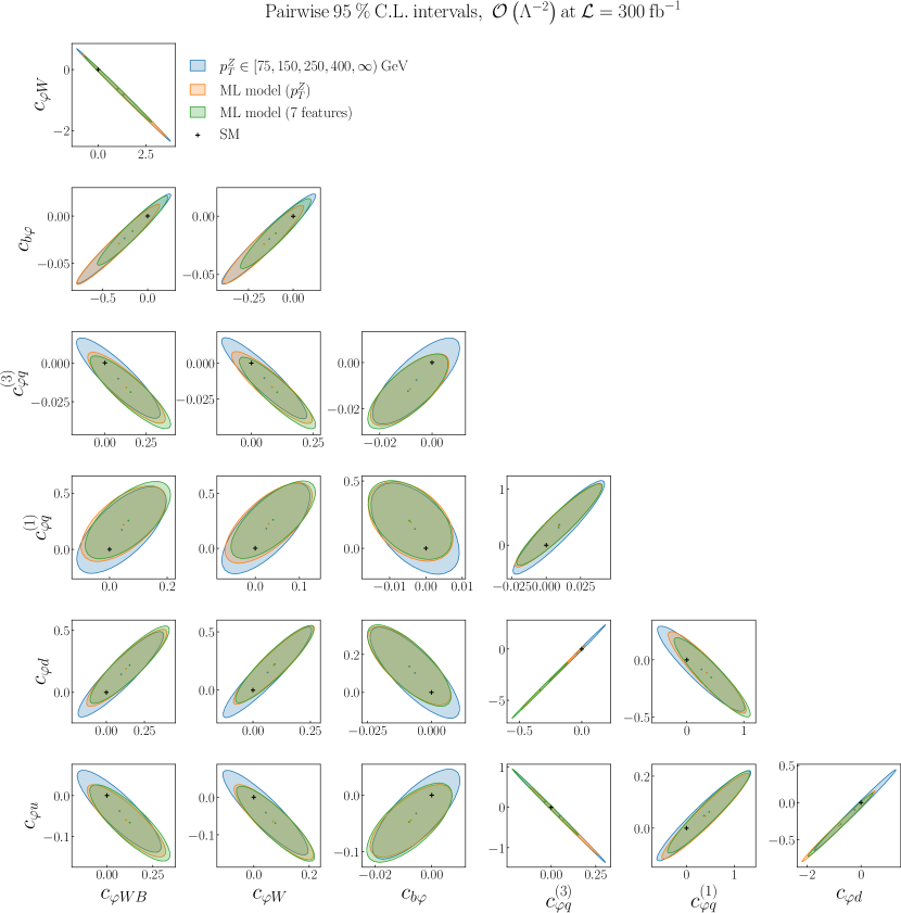
Figure 5.6: Pair-wise 95% CL contours obtained from two-parameter fits in case of $pp\rightarrow hZ\rightarrow b\bar{b}\ell^{+}\ell^{-}$ at the linear level in the EFT expansion for the $n_{\rm eft}=7$ Wilson coefficients relevant for the description of this process. For each panel, the contribution from the operators not displayed is set to zero. We compare the bounds obtained from a binned $p_{T}^{Z}$ distribution with those from two ML unbinned observables, first when only $p_{T}^{Z}$ is used for the training and then when $n_{k}=7$ kinematic features are used to parametrize the likelihood ratio.

Fig. 5.6 displays the pair-wise 95% CL contours obtained from two-parameter fits of $pp\rightarrow hZ\rightarrow b\bar{b}\ell^{+}\ell^{-}$ pseudo-data at the linear level in the EFT expansion. In these two-parameter fits, for each panel the contribution from the operators not being shown is set to zero. The choice of displaying the outcome of two-parameter fits, rather than a full marginalized analysis, is motivated by the fact that the linear EFT analysis is not stable when all coefficients are simultaneously considered due to quasi-flat directions and strong operator correlations. This restriction can be lifted once we account for quadratic effects.

We show the bounds obtained from a binned $p_{T}^{Z}$ distribution, with $p_{T}^{Z}$ being the dilepton transverse momentum, where the choice of binning is given by

$$p_{T}^{Z}\in[75,150,250,400,\infty)\,,$$ (5.2)

consistent with the definitions entering the Simplified Template Cross Section (STXS) [84] adopted by the LHC Higgs Working Group. These binned bounds are compared with those from two ML unbinned observables, first when only the dilepton transverse momentum $p_{T}^{Z}$ is used for the training and second when the full set of $n_{k}=7$ kinematic features is used to parametrize the likelihood ratio. As in the case of top quark production, comparing the constraints from the binned observable with those from the unbinned one trained on the same feature quantifies the information loss incurred by the binning procedure, while comparing one feature with multivariate unbinned observables determines the information loss associated to the use of a restricted set of kinematic features

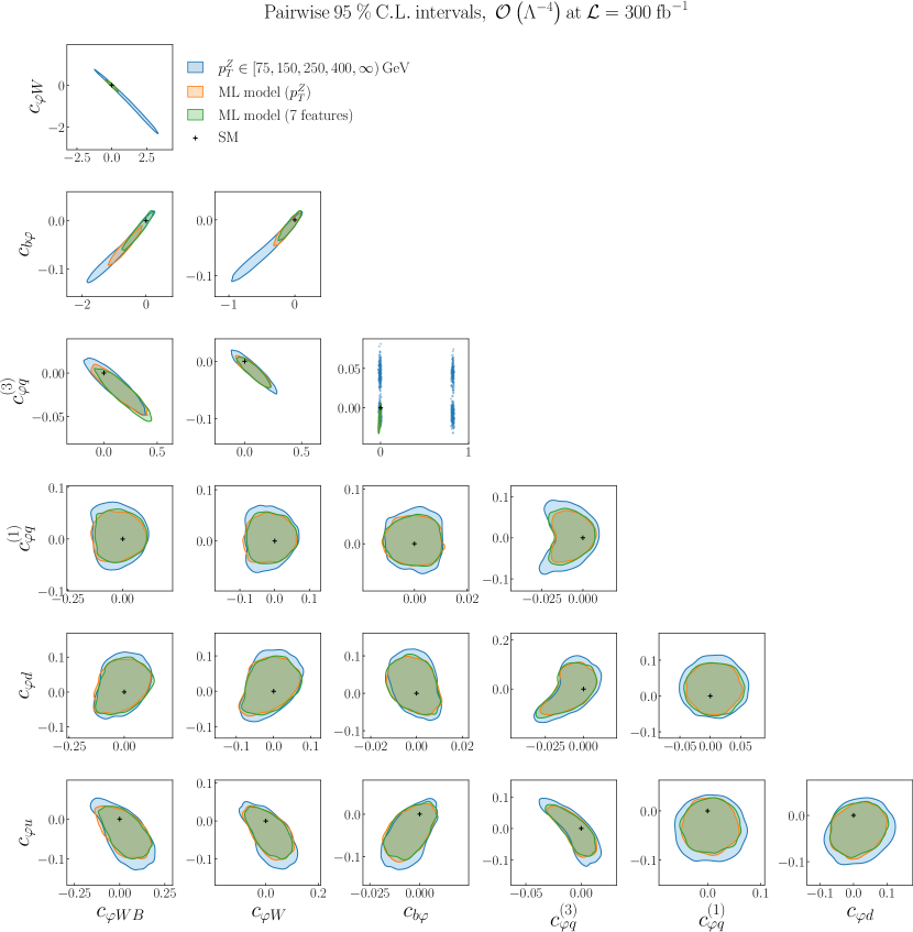
Figure 5.7: Same as Fig. 5.6 for the case in which the EFT calculations also include the quadratic $\mathcal{O}(\Lambda^{-4})$ corrections.

At this linear EFT level, the improvement in the constraints provided by unbinned observables as compared to their binned $p_{T}^{Z}$ counterparts is moderate, yet appreciable, for most operator pairs. The most stringent bounds are those associated with unbinned observables, and the constraints provided by the multivariate unbinned observable based on 7 kinematic features are similar to those associated to the single-feature version trained on $p_{T}^{Z}$. One observes strong correlations between all operators pairs being considered, indicating quasi-flat directions: these will be broken either by quadratic corrections or by adding other processes sensitive to the same SMEFT operators, such as vector-boson scattering and diboson data [16]. The analysis of Fig. 5.6 indicates that for the $hZ\rightarrow b\bar{b}\ell^{+}\ell^{-}$ process the chosen binning in $p_{T}^{Z}$ provides the bulk of the information on the EFT operators, with minor additional improvements provided by the unbinned multivariate analysis.

Therefore, for this specific process the formalism developed in this work provides a diagnosis tool that determines when and under which circumstances a binned analysis provides information on the EFT parameter space close to the optimal one, represented here by the bounds associated to the unbinned multivariate observable. This finding illustrates the two-fold applicability of our formalism: whenever unbinned multivariate observables markedly improve over their binned counterparts, they can be included in the global SMEFT fit, otherwise one obtains quantitative confirmation that the information provided by the specific settings of the binned observables is sufficiently close to the optimal amount.

The results of the corresponding analyses of the impact of unbinned observables in the $hZ\rightarrow b\bar{b}\ell^{+}\ell^{-}$ process in the presence of quadratic EFT corrections are shown in Fig. 5.7 for the case of two-parameter fits, and in Fig. 5.8 for the case where all relevant operators are considered simultaneously, producing marginalized constraints on each operator pair. As mentioned above, the latter is possible since quadratic corrections break up the EFT parameter degeneracies that destabilize the inference procedure in the linear case.

Considering first the results of Fig. 5.7, one finds that on the one hand the improvement associated to the use of unbinned observables is more marked as compared to the linear EFT case. On the other hand, the addition of other kinematic features on top of $p_{T}^{Z}$ does not modify the discrimination power of the unbinned observables, as also observed for the linear analysis. For specific operator pairs, there is a clear reduction in the parameter bounds based on the unbinned observables, for instance in the case of the $\left(c_{\varphi W},c_{\varphi WB}\right)$ pair. We note that enhanced discrimination in the presence of quadratic EFT corrections can be partially attributed to energy-growing effects in the $p_{T}^{Z}$ distribution which are more pronounced as compared to the linear level.

Another benefit associated to unbinned observables in this specific process is that of breaking degeneracies leading to a double maximum structure in the posterior distribution. Indeed, the unbinned observables removes the second minimum present in the binned analysis arising from a bimodal distribution in the ($c_{\varphi q}^{(3)}$, $c_{b\varphi}$)-plane and corresponding to the scenario where the quadratic EFT contribution becomes of the same magnitude and opposite sign as the linear term and hence canceling it. We also note that, as opposed to the $t\bar{t}$ production case, for the $hZ$ process, even with unbinned observables, one ends up with some operator pairs that exhibit relatively large correlations which would thus only be broken by adding other processes to the fit. The results of Fig. 5.7 highlight how in general the relevance of considering unbinned observables depends not only on the processes and on the order in the EFT expansion, but also on the specific directions in the EFT parameter space in which one is interested.

The results of Fig. 5.7 display good agreement between unbinned observables trained only on $p_{T}^{Z}$ and on the full set of $n_{k}=7$ kinematic features, suggesting that a multivariate analysis does not appear to be beneficial for this process. However, this interpretation turns out to be an artifact of restricting the analysis to the case of two-parameter fits, and a different picture emerges in the case of the marginalized analysis results displayed in Fig. 5.8. The impact on the EFT parameter space of adopting unbinned observables is more important now, leading in some cases to stringent bounds improved by up to a factor 5 as compared to the binned results, for instance for the $c_{\varphi W}$ operator. Furthermore, one can also appreciate the improved constraints associated to the multivariate observable based on the full set of kinematic features as compared to the single-feature unbinned observable. We also note how the degenerate minimum associated to the bottom Yukawa operator present in the binned analysis, now for all operator pairs, goes away when unbinned observables are considered. The comparison of Figs. 5.7 and 5.8 emphasizes that bounds obtained in two-parameter fits, neglecting the effects of other operators, will in general overestimate the EFT constraints associated to a given dataset.

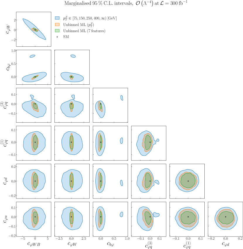
Figure 5.8: Same as Fig. 5.7 now where the $95\%$ CL contours are obtained from the marginalisation over the full posterior probability distribution, rather than from two-parameter fits.

To summarize, as in the case of top quark pair production, for $hZ$ production the use of unbinned multivariate observables is advantageous in constraining the EFT parameter space. Our analysis indicates that the choice of $p_{T}^{Z}$ binning adopted by the STXS analysis is close to being optimal, especially in the linear case, at least for the assumed integrated luminosity and for two-parameter fits. When considering a full marginalized analysis in the presence of quadratic EFT corrections, marked improvements associated first to the use of unbinned observables and second to that of multiple kinematic features are obtained. The use of unbinned observables also results in the removal of degenerate minima corresponding to solutions where the quadratic EFT correction approximately cancels out the linear one. The comparison between the output of the two-parameter and the marginalized fits emphasizes the crucial importance of carrying out global SMEFT interpretations, since setting to zero a subset of operators that contribute to a given process is likely to overestimate its impact in the EFT parameter space.

5.5 Methodological uncertainties

The results for the unbinned observables derived so far are obtained from EFT parameter inference carried out with Eq. (3.19), the parametrization of the likelihood ratio, as described in Sect. 5.1. As explained in Sect. 3.3, within our approach, rather than a single best model, we produce a distribution of models, denoted as replicas, each of them trained on a different set of Monte Carlo events. Hence the end result of our procedure is Eq. (3.23), the representation of the probability distribution of the likelihood ratio $\{\hat{r}^{(i)}_{\sigma}(\bm{x},\bm{c})\}$ composed of $N_{\rm rep}$ equiprobable replicas. The spread of this distribution provides a measure of methodological and procedural uncertainties associated e.g. to finite training datasets and inefficiencies of the optimization and stopping algorithms. Results presented in Sects. 5.2–5.4 are based on using the median of the replica distribution $\{\hat{r}^{(i)}_{\sigma}(\bm{x},\bm{c})\}$ to determine the bounds in the EFT parameter space, and here we assess the impact of methodological uncertainties by displaying results for parameter inference based on the full distribution of replicas of the likelihood ratio parametrization.

Figs. 5.9 and 5.10 display the bounds in the parameter space obtained for particle-level top-quark pair and $hZ$ associated production, respectively, from the unbinned multivariate observables based on the complete set of kinematic features and in the case of theory simulations that include quadratic EFT corrections. We compare results for parameter inference based on the median of the replica distribution $\{\hat{r}^{(i)}_{\sigma}(\bm{x},\bm{c})\}$, which coincide with those of Figs. 5.5 and 5.8, with results based on the full distribution of replicas. Namely, in the latter case one starts from the $N_{\rm rep}$ individual replicas of the profile likelihood ratio functions and performs Nested Sampling inference on each of them, to subsequently combine the resulting samples and estimate the posterior distribution by means of the KDE method. In this manner, the differences between the contours shown in Figs. 5.9 and 5.10 provide an estimate of how methodological uncertainties associated to the machine learning training procedure impact the derived bounds in the EFT parameter space.

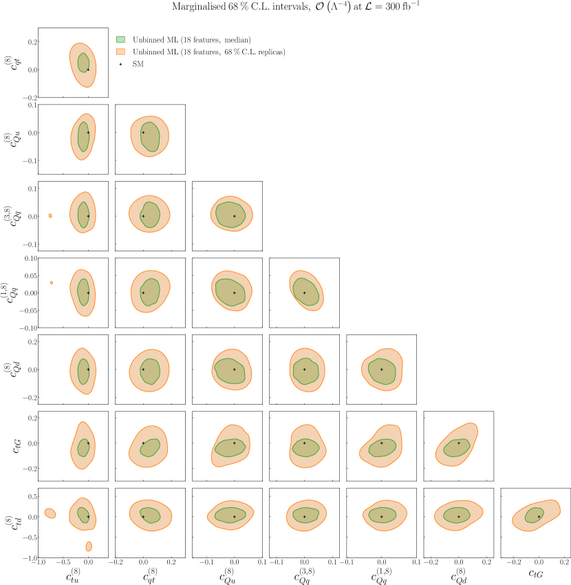
Figure 5.9: Same as Fig. 5.5 for the 68% CL contours in the EFT parameters obtained with the unbinned multivariate observable for particle-level top-quark pair production. We compare the bounds obtained from the median of the replica distribution of the likelihood ratio parametrization, as done in Fig. 5.5, with the corresponding bounds obtained taking into account the full replica distribution.

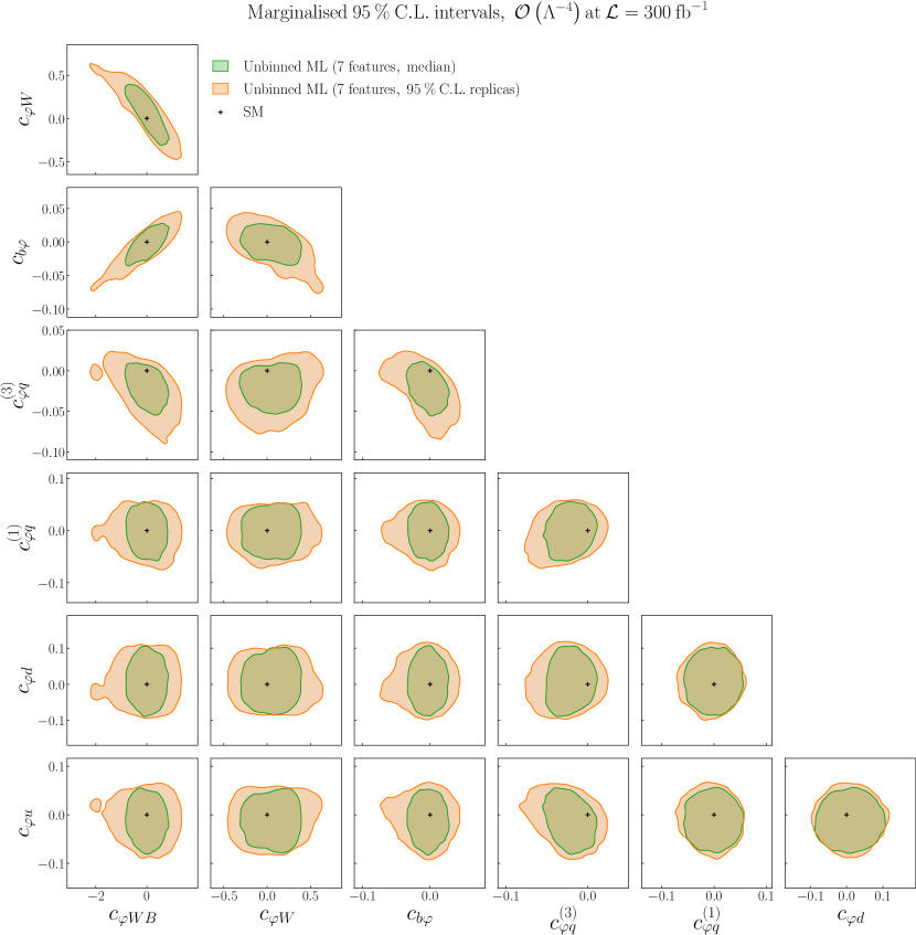
Figure 5.10: Same as Fig. 5.9 for Higgs associated production with a $Z$ boson, now for the 95% CL contours.

Inspection of Figs. 5.9 and 5.10 and comparison with the corresponding bounds displayed in Figs. 5.5 and 5.8 confirm that these procedural uncertainties, as estimated with the replica method, do not modify the qualitative results obtained from the median of the likelihood ratio. In particular, the observation that bounds obtained using multivariate unbinned observables are much stronger than those based on unbinned models based on one or two kinematic features, which is common to both the $t\bar{t}$ and $hZ$ processes, remains valid once replica uncertainties are accounted for. Furthermore, we note that in principle it is possible to reduce the spread of the replica distribution by training on higher-statistics samples and adopting more stringent stopping criteria. In this respect, our approach provides a strategy to quantify under which conditions the computational overhead required to achieve more accurate machine learning trainings is justified from the point of view of the impact on the EFT coefficients. This said, these results also indicate that in realistic scenarios based on finite training samples methodological uncertainties cannot be neglected, and should be accounted for in studies of the impact of ML-based observables in EFT analyses.

6 Summary and outlook

The general problem of identifying novel types of measurements which, given a theoretical framework, provide enhanced or even maximal sensitivity to the parameters of interest is ubiquitous in modern particle physics. Constructing such optimized observables has a two-fold motivation: on the one hand, to achieve the most stringent constraints on the model parameters from a specific process, and on the other hand, to provide bounds on the maximum amount of information that can be extracted from the same process. Optimized observables can hence be used to design traditional observables in a way that approaches or saturates the limiting sensitivity by highlighting the best choices of binning and kinematic features.

In this work, we have presented a new framework for the design of optimal observables for EFT applications at the LHC, making use of machine learning techniques to parametrize multivariate likelihoods for an arbitrary number of higher-dimensional operators. To illustrate the reach of our method, we have constructed multivariate unbinned observables for top-quark pair production and Higgs production in association with a $Z$ boson. We have demonstrated how these observables either lead to a significant improvement in the constraints on the EFT parameter space, or indicate the conditions upon which a traditional binned analysis already saturates the EFT sensitivity.

The ML4EFT framework presented in this work and the accompanying simulated event samples are made available as an open source code which can be interfaced with existing global EFT fitting tools such as SMEFiT, FitMaker [17], HepFit [14], and Sfitter [83]. Its scaling behavior with the number of parameters, together with its parallelization capabilities, make it suitable for its integration within global EFT fits which involve several tens of independent Wilson coefficients. While in its current implementation the parametrized likelihood ratios are provided in terms of the output of the trained network replicas, work in progress aims to tabulate this output in terms of fast interpolation grids, as done customarily in the case of PDF analyses [85, 86, 87, 88]. The resulting interpolated unbinned likelihood ratios can then be combined with Gaussian or Poissonian binned measurements within a global fit. While currently ML4EFT can only be used in combination with simulated Monte Carlo pseudo-data, all of the ingredients required for the analysis of actual LHC measurements are already in place.

The results presented in this work could be extended along several directions. First, one could include experimental and theoretical correlated systematic uncertainties, as required for the interpretation of measurements which are not dominated by statistics. Second, other machine learning algorithms could be adopted, which may offer performance advantages as compared to those used here: one possibility could be graph neural networks [89, 90] which make possible varying the kinematic features used for the training on an event-by-event basis. Third, ML4EFT could be applied to more realistic final states with higher order corrections, such as by means of NNLO+PS simulations of $t\bar{t}$ and $hV$ [91, 92, 93], and accounting for detector effects to bridge the gap between the theory predictions and the experimentally accessible quantities. It would also be interesting to compare the performance of different approaches to construct ML-assisted optimized observables for EFT applications in specific benchmark scenarios.

Beyond hadron colliders, the framework developed here could also be relevant to construct optimal observables for EFT analyses in the case of high-energy lepton colliders, such as electron-positron collisions at CLIC [94, 95] or at a multi-TeV muon collider [96, 97, 98]. As mentioned, statistically optimal observables were actually first designed for electron-positron colliders, where the simpler final state facilitates the calculation of the exact event likelihood for parameter inference [21, 22, 23]. These methods may not be suitable to the high multiplicity environment of multi-TeV lepton colliders, in particular due to the complex pattern of electroweak radiation. Therefore, the ML4EFT method could provide a suitable alternative to construct unbinned multivariate observables achieving maximal EFT sensitivity at high-energy lepton colliders.

In addition to applications to the SMEFT, our framework could also be relevant to other types of theory interpretations of collider data such as global PDF fits. In particular, PDFs at large values of Bjorken-$x$ are poorly constrained [99] due to the limited amount of experimental data available. This lack of knowledge degrades the reach of searches for both resonant and non-resonant new physics in the high-energy tail of differential distributions, as recently emphasized for the case of the forward-backward asymmetry in neutral-current Drell-Yan production [100]. Given that measurements of these high-energy tails are often dominated by statistical uncertainties, the ML4EFT method could be used to construct unbinned multivariate observables tailored to constrain large-$x$ PDFs at the LHC. Our method could also be applied in the context of a joint extraction of PDFs and EFT coefficients [101, 102, 103, 104, 105], required to disentangle QCD effects from BSM ones in kinematic regions where they potentially overlap, such as large Bjorken-$x$.

Acknowledgments

We are grateful to Gaia Grosso, Wouter Verkerke, and Andrea Wulzer for stimulating discussions. The work of J. t. H is supported by the Dutch Science Council (NWO) via an ENW-KLEIN-2 project. The research of J. R. is partially supported by NWO and by an ASDI grant of The Netherlands eScience Center. The research of V. S. is supported by the Generalitat Valenciana PROMETEO/2021/083 and the Ministerio de Ciencia e Innovacion PID2020-113644GB-I00. The work of M. M. is supported by the European Research Council under the European Union’s Horizon 2020 research and innovation Programme (grant agreement n.950246) and in part by STFC consolidated grant ST/T000694/1. The work of R. G. A. is supported by the ERC Starting Grant REINVENT-714788 and by Grant DataSMEFT23 (PNRR - DM 247 08/22).

Appendix A The ML4EFT framework

The ML4EFT framework presented in this work is an open source Python code designed to facilitate the integration of unbinned multivariate observables into fits of Wilson coefficients in the SMEFT. It is based on machine learning regression and classification techniques to parameterize high-dimensional likelihood ratios as required to carry out parameter inference in the context of global SMEFT analyses. ML4EFT is made available via the Python Package Index (pip) and can be installed directly by running

pip install ml4eft

or alternatively the code can be downloaded from its public GitHub repository,

https://github.com/LHCfitNikhef/ML4EFT.git

and then installed from source following the installation instructions. The framework is documented in a dedicated website

https://lhcfitnikhef.github.io/ML4EFT,

where, in addition, one can find a self-standing tutorial (which can also be run in Google Colab) where the user is guided step by step in how unbinned multivariate observables can be constructed given a choice of EFT coefficients and of final-state kinematic features.

In the same website we also provide links to the main results of this paper presented in Sect. 5, including the likelihood ratio parametrizations that have been obtained for the two processes ($t\bar{t}$ and $hZ$) considered here. We also include there animations demonstrating the training of the neural networks, such as e.g.

https://lhcfitnikhef.github.io/ML4EFT/sphinx/build/html/results/ttbar_analysis_parton2.html#overview

Additional unbinned multivariate observables to be constructed in the future using our framework will be added to the same page. Furthermore, we also plan to tabulate the neural network outputs using fast grid techniques so that these observables can be stand-alone integrated in global fits without the need to link the actual ML4EFT code.

Appendix B The unbinned Asimov data set

The Asimov data set was first introduced in [70] as an efficient method of obtaining the distribution of the profile likelihood ratio $q_{\bm{c}}$, Eq. (2.8), under the alternative hypothesis $\bm{c}^{\prime}\neq\bm{c}$ without having to resort to computationally expensive MC simulations. Since then, it has become part of the standard analysis toolkit at the LHC to determine e.g. expected exclusion limits. The analysis of [70] considers the Asimov data set applied to binned observables and here, by adopting a simple EFT-like toy model, we present its generalisation to a continuous Asimov data set. This makes possible determining expected exclusion limits in a sampling free way by extending the results of [70] to unbinned observables. While we do not make use of this unbinned Asimov data set in the results presented in this work, this derivation can play an important role in the general discussion of unbinned multivariate measurements for EFT studies.

Let us consider a kinematic variable $x$ (e.g. the invariant mass) restricted to $x\in X=[1,5]$ and distributed according to a probability distribution $f_{\sigma}(x,c)$. The EFT toy model is chosen such that the effect of the EFT on the kinematic variable is an enhancement in the tail of the distribution $f_{\sigma}(x,c)$ with respect to the SM, as is common in many EFT scenarios. The distribution $f_{\sigma}(x,c)$ is defined as

$$f_{\sigma}(x,c)\equiv{{1}\over{\sigma(X,c)}}\left[f_{\sigma}^{(\mathrm{sm})}(x)+0.1c\cdot f_{\sigma}^{(\mathrm{eft})}(x)\right],$$ (B.1)

with

$$f_{\sigma}^{(\mathrm{sm})}(x)={{1}\over{\sigma^{(\mathrm{sm})}}}{{(1+x^{2})\sqrt{x^{2}-1}}\over{x^{4}}}$$ (B.2)

and

$$f_{\sigma}^{(\mathrm{eft})}(x)={{1}\over{\sigma^{(\mathrm{eft})}}}{{(x^{2}-1)^{3/2}}\over{x}},$$ (B.3)

where $f_{\sigma}^{(\mathrm{sm})}(x)$ and $f_{\sigma}^{(\mathrm{eft})}(x)$ are both separately normalized by $\sigma^{(\mathrm{sm})}$ and $\sigma^{(\mathrm{eft})}$ respectively such that the overall normalization constant $\sigma(X,c)$ is given by

$$\sigma(X,c)=1+0.1c.$$ (B.4)

The number of expected events $\nu(c)$ is determined from $\sigma(X,c)$ and the luminosity $L$, which we set to $L=1000$ unless otherwise specified. We work with dimensionless parameters throughout this toy example.

In Fig. B.1(a) we show the distribution $f_{\sigma}(x,c)$ at $c=0$ and $c=1$, corresponding to the SM and the EFT hypotheses respectively. One can see a clear energy growing effect in the tail of the EFT distribution. The histograms have been constructed using accept/reject sampling and contain 1M samples from each hypothesis. These will serve as our parent data sets from which we will take subsequent samples in the following.

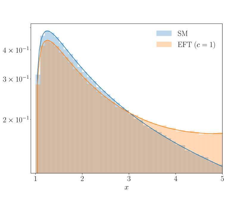
(a)

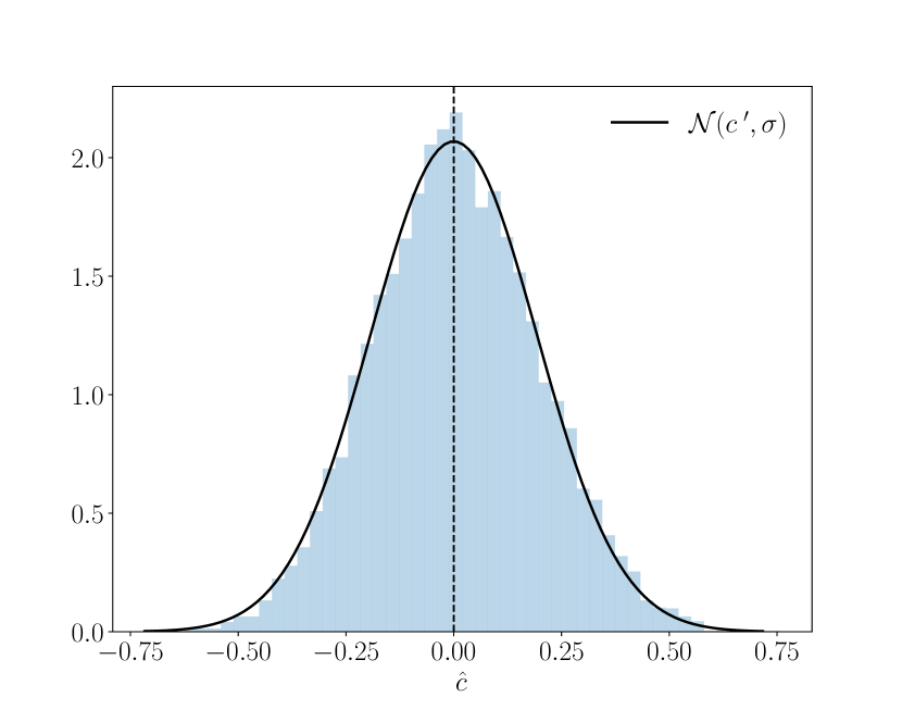
(b)

Figure B.1: Left: the probability distribution $f_{\sigma}(x,c)$ from Eq. (B.1) at $c=1$ and $c=0$, corresponding to the EFT and SM respectively. Right: the MLE $\hat{c}$ under the SM follows a Gaussian distribution centered around $c^{\prime}$ with standard deviation $\sigma$.

Now, taking the EFT at $c=1$ as our null hypothesis, the goal is to compute the expected significance at which we can either accept or reject the null assuming data generated under the SM (the alternative hypothesis). We adopt the PLR from Eq. (2.8) as our test statistic,

$$q_{c}=-2\left[\nu(\hat{c})-\nu(c)+\sum_{i=1}^{N_{\mathrm{ev}}}\log{{\nu(c)f_{\sigma}(x,c)}\over{\nu(\hat{c})f_{\sigma}(x,\hat{c})}}\right],$$ (B.5)

whose distribution under the SM and the EFT we denote by $\mathrm{pdf}(q_{c}|0)$ and $\mathrm{pdf}(q_{c}|c)$ respectively. One can imagine repeatedly drawing toy datasets from the SM parent data set, computing $q_{c}$, and evaluating its $p$-value under the null. The median p-value then serves as a measure of expected sensitivity. Moreover, since the $p$-value is monotonic with $q_{c}$, it is equivalent to report the $p$-value associated with the median $q_{c}$ under the SM, denoted $\mathrm{Med}[q_{c}|0]$,

$$p_{c,\mathrm{med}}=\int_{q_{c,\mathrm{med}}}^{\infty}\mathrm{pdf}(q_{c}|c)dq_{c}\qquad\text{with}\qquad q_{c,\mathrm{med}}\equiv\mathrm{Med}[q_{c}|0].$$ (B.6)

From the above discussion it becomes clear one not only needs $\mathrm{pdf}(q_{c}|c)$, which follows a $\chi^{2}$-distribution as discussed in Sec. 2.1, but also $\mathrm{pdf}(q_{c}|c^{\prime})$ with $c^{\prime}\neq c$. At this point we employ Wald’s theorem [106], which states that for a data set of size $N$ generated under $f_{\sigma}(x,c^{\prime})$, the PLR $q_{c}$ can be approximated by

$$q_{c}={{(c-\hat{c})^{2}}\over{\sigma^{2}}}+\mathcal{O}\left(1/\sqrt{N}\right),$$ (B.7)

where $\hat{c}$ follows a normal distribution with mean $c^{\prime}$ and a variance $\sigma^{2}$, i.e. $\hat{c}\sim\mathcal{N}(c^{\prime},\sigma)$. Not only does the approximation provided by Wald’s theorem depend on a large sample size $N$ [106], but the approximation improves as $c\rightarrow\hat{c}\simeq c^{\prime}$. This can be understood by Taylor expanding Eq. (2.8) about $\hat{c}$. Defining $\Delta\equiv(c-\hat{c})$, we find

$$q_{c}=-2\log{{\mathcal{L}(c)}\over{\mathcal{L}(\hat{c})}} =-2\log\left[1+{{1}\over{2\mathcal{L}(\hat{c})}}\left.{{\partial^{2}\mathcal{L}}\over{\partial c^{2}}}\right|_{c=\hat{c}}\Delta^{2}+\mathcal{O}\left(\Delta^{3}\right)\right]$$

$$=-{{1}\over{\mathcal{L}(\hat{c})}}\left.{{\partial^{2}\mathcal{L}}\over{\partial c^{2}}}\right|_{c=\hat{c}}\Delta^{2}+\mathcal{O}\left(\Delta^{3}\right)={{\Delta^{2}}\over{\sigma^{2}}}+\mathcal{O}\left(\Delta^{3}\right),$$

where on the last line we have used that

$${{1}\over{\sigma^{2}}}=-\left.{{\partial^{2}\log\mathcal{L}}\over{\partial c^{2}}}\right|_{c=\hat{c}}.$$ (B.8)

Let us define $q_{c}^{\mathrm{wald}}$ as the leading order approximation of Eq. (B.7),

$$q_{c}^{\mathrm{wald}}\equiv{{(c-\hat{c})^{2}}\over{\sigma^{2}}}.$$ (B.9)

Recalling that $\hat{c}\sim\mathcal{N}(c^{\prime},\sigma)$, we note that $q_{c}^{\mathrm{wald}}$ corresponds to a squared Gaussian random variable with unit variance and non-zero mean. This is known to follow a non-central $\chi^{2}$ distribution [70],

$$\mathrm{pdf}(q_{c}^{\mathrm{wald}}|c^{\prime})={{1}\over{2\sqrt{q_{c}}}}{{1}\over{\sqrt{2\pi}}}\left[\exp\left(-{{1}\over{2}}\left(\sqrt{q_{c}}+\sqrt{\Lambda}\right)^{2}\right)+\exp\left(-{{1}\over{2}}\left(\sqrt{q_{c}}-\sqrt{\Lambda}\right)^{2}\right)\right]\;,$$ (B.10)

with the non-centrality parameter $\Lambda$ given by

$$\Lambda={{(c-c^{\prime})^{2}}\over{\sigma^{2}}}.$$ (B.11)

Note how Eq. (B.10) reduces to a central $\chi^{2}$ distribution under the null hypothesis, i.e. when $c^{\prime}=c$, as dictated by Wilk’s theorem.

The problem of obtaining $\mathrm{pdf}(q_{c}|c^{\prime})$ with $c^{\prime}\neq c$ is now reduced to the question of determining the non-centrality parameter $\Lambda$ to be used in Eq. (B.10). We can construct this using MC toys: for example, in Fig. B.1(b) we show the distribution of $\hat{c}$ under the SM, obtained using $10$K toy data sets containing $n_{\rm ev}$ samples each, where $n_{\rm ev}$ is drawn from $\mathrm{Pois}(\nu(0))$ each time a new experiment is run. The distribution in Fig. B.1(b) gives $\sigma=0.19$, resulting in $\Lambda_{\mathrm{MC}}=27.12$. However, although constructing $\mathrm{pdf}(\hat{c}|c^{\prime})$ using MC toys gives us the info we need to extract $\Lambda$, it is computationally highly inefficient. This is especially so in case one needs to perform scans along different $c^{\prime}$, e.g. to find expected exclusion limits.

This is where the Asimov data set enters as an efficient tool to obtain $\Lambda$ [70]. The Asimov data set is defined such that one recovers the true value of $c$ during maximum likelihood estimation, i.e. $\hat{c}=c$. In the case of a Poissonian likelihood $\mathcal{L}_{\mathrm{pois}}$ defined as in Eq. (2.4), the MLE $\hat{c}$ satisfies

$$\left.{{d\log\mathcal{L}_{\mathrm{pois}}}\over{dc}}\right|_{c=\hat{c}}=\left.{{d}\over{dc}}\left\{-2\sum_{i=1}^{n_{\mathrm{bins}}}\left[n_{i}\log\nu_{i}(c)-\nu_{i}(c)\right]\right\}\right|_{c=\hat{c}}=0\,.\\$$ (B.12)

The Asimov data set is then constructed such that Eq. (B.12) implies $\hat{c}=c$, which can only be true if $n_{i}=\nu_{i}(c)$. Therefore, we define the Asimov data set under the hypothesis $c$ as

$$\mathcal{D}_{\mathrm{Asimov}}\equiv\{n_{i,A}\}=\{\nu_{i}(c)\}.$$ (B.13)

The non-centrality parameter $\Lambda$ can then be found by evaluating $q_{c}$ on the Asimov data set corresponding to the alternative hypothesis $c^{\prime}$, i.e. $n_{i,A}=\nu_{i}^{\prime}$,

$$\Lambda_{\mathrm{A,binned}}=q_{c}(\{n_{i,A}\})=-2\sum_{i=1}^{n_{\mathrm{bins}}}\left[\nu_{i}^{\prime}\log\left({{\nu_{i}}\over{\nu_{i}^{\prime}}}\right)-\nu_{i}+\nu_{i}^{\prime}\right],$$ (B.14)

where we have used the fact that $\hat{c}=c^{\prime}$ and therefore $\hat{\nu_{i}}=\nu_{i}^{\prime}$ by construction. The relationship between $\Lambda$ and $q_{c}$ can be understood by comparing Eqs. (B.9) and (B.11) and noting that they coincide when $\hat{c}=c^{\prime}$.

Now, one could wonder how Eq. (B.14) generalizes to the case of unbinned data. An intuitive starting point is to study the behavior of $\Lambda_{\mathrm{A,binned}}$ as one increases the number of bin insertions, and by doing so we find that after $\sim 10$ bins, $\Lambda_{\mathrm{A,binned}}$ converges to a stable value. Encouraged by this convergence, we take the infinitely narrow bin limit of Eq. (B.14),

$$\Lambda_{\mathrm{A,binned}} =-2\sum_{i=1}^{n_{\mathrm{bins}}}\left[\nu_{i}^{\prime}\log\left({{\nu_{i}}\over{\nu_{i}^{\prime}}}\right)-\nu_{i}+\nu_{i}^{\prime}\right]$$

$$\rightarrow-2\int_{-\infty}^{\infty}\left[\nu(c^{\prime})f_{\sigma}(x,c^{\prime})\log\left({{\nu(c)f_{\sigma}(x,c)}\over{\nu(c^{\prime})f_{\sigma}(x,c^{\prime})}}\right)-\nu(c)f_{\sigma}(x,c)+\nu(c^{\prime})f_{\sigma}(x,c^{\prime})\right]dx\equiv\Lambda_{\mathrm{A,unbinned}},$$ (B.15)

where we have sent $\nu_{i}(c)\rightarrow\nu(c)f_{\sigma}(x,c)dx$. Evaluating the integral in Eq. (B.15) gives $\Lambda_{\mathrm{A,unbinned}}=22.11$.

In Fig. B.2 we select three benchmark points at which to visualize the distribution $\mathrm{pdf}(q_{c}|c^{\prime})$: the SM ($c=0$) and the EFT at $c=0.5$, $c=1$. Firstly, the green histogram shows the distribution of $q_{c}$ evaluated on data following the EFT hypothesis. The distribution is obtained by repeatedly drawing samples of size $n_{ev}\sim\mathrm{Pois}(\nu(c))$ from the parent EFT dataset and calculating $q_{c}$ as given by the PLR in Eq. (2.8). The solid green curve indicates the distribution of a $\chi^{2}$ with 1 degree of freedom. We find excellent agreement between the green curve and histogram, as expected from Wilk’s theorem.

A similar procedure is used to obtain the blue histogram, this time corresponding to the SM hypothesis. We repeatedly draw samples of size $n_{ev}\sim\mathrm{Pois}(\nu(0))$ from the parent SM dataset and calculate $q_{c}$ as given by the PLR in Eq. (2.8). The resulting distribution is denoted by $\mathrm{pdf}(q_{c}^{\mathrm{exact}}|c)$. In contrast, the orange histogram is produced using the approximation given by Wald’s theorem in Eq. (B.9). For each sample drawn, we evaluate $q_{c}^{\mathrm{wald}}$ rather than the full expression for $q_{c}$, resulting in the distribution $\mathrm{pdf}(q_{c}^{\mathrm{wald}}|c)$. We notice a non-negligible difference in the distributions of $q_{c}$ before and after employing Wald’s theorem. As expected, this is due to the fact that the neglected $\mathcal{O}(\Delta^{3})$ term is in fact quite sizable, being on the order of a few percent. In Fig. B.2(b) we show that the difference between $\mathrm{pdf}(q_{c}^{\mathrm{wald}}|c)$ and $\mathrm{pdf}(q_{c}^{\mathrm{exact}}|c)$ gets smaller when we move to a smaller $\Delta$, corresponding to $c=0.5$.

Finally, we turn to the solid blue and orange curves. In orange, we plot the distribution of the non-central $\chi^{2}$ as given by Eq. (B.10), setting the non-centrality parameter $\Lambda$ to $\Lambda_{\mathrm{MC}}=27.12$. We find good agreement between the orange curve and the orange histogram, as expected from the fact that both employ Wald’s theorem. The blue curve, on the other hand, indicates the non-central $\chi^{2}$ distribution evaluated at $\Lambda_{\mathrm{A,unbinned}}=22.11$ as calculated using Eq. (B.15). In this case the agreement between the blue curve and histogram is non-trivial: it indicates that the non-centrality parameter evaluated on the unbinned Asimov dataset provides an excellent description of the distribution of the PLR $q_{c}$ evaluated on unbinned data. This is the case both at $c=1$ and $c=0.5$, and provides a validation of the expression for $\Lambda_{\mathrm{A,unbinned}}$ determined in Eq. (B.15). This agreement suggests Eq. (B.15) includes some higher order contributions that are otherwise omitted if one adopts instead Eq. (B.11). This was also conjectured in [70].

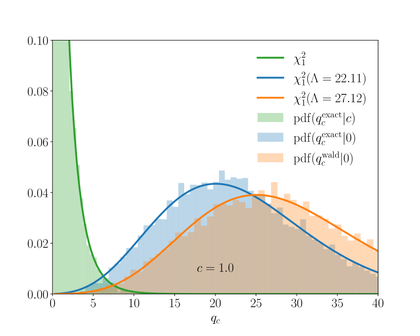
(a)

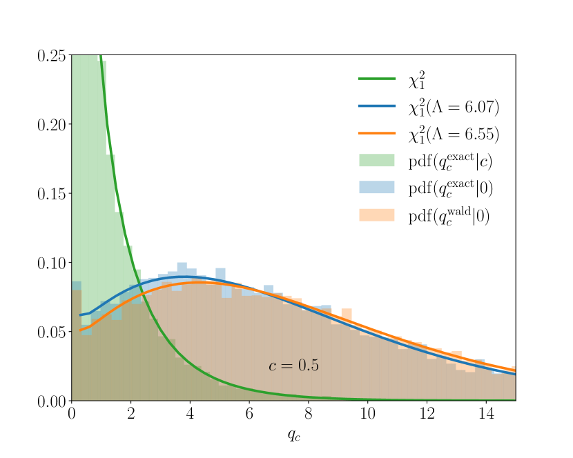
(b)

Figure B.2: The distributions of $q_{c}$ under the EFT and the SM hypotheses for $c=1.0$ (a) and $c=0.5$ (b). The blue curve agrees well with the distribution $\mathrm{pdf}(q_{c}^{\mathrm{exact}}|c)$, indicating that the distribution of $q_{c}$ is well described by the non-central $\chi^{2}$ evaluated with non-centrality parameter $\Lambda_{\mathrm{A,unbinned}}$. We notice a disagreement between the distribution of $q_{c}^{\mathrm{exact}}$ and $q_{c}^{\mathrm{wald}}$, meaning that neglecting the higher order corrections in Wald’s theorem leads to sizable differences. On the right (b) it can be seen that this difference gets smaller when $c\rightarrow c^{\prime}$, i.e. $\Delta\rightarrow 0$.

Finally, Eq. (B.15) generalizes straightforwardly to the case of $n_{\rm p}$ model parameters $\bm{c}$, and to the case of a multi-dimensional vector $\bm{x}$ of kinematic variables

$$\Lambda_{\mathrm{A,unbinned}}=\int_{-\infty}^{\infty}\left[\nu(\bm{c}^{\prime})f_{\sigma}(\bm{x},\bm{c}^{\prime})\log\left({{\nu(\bm{c})f_{\sigma}(\bm{x},\bm{c})}\over{\nu(\bm{c}^{\prime})f_{\sigma}(\bm{x},\bm{c}^{\prime})}}\right)-\nu(\bm{c})f_{\sigma}(\bm{x},\bm{c})+\nu(\bm{c}^{\prime})f_{\sigma}(\bm{x},\bm{c}^{\prime})\right]d\bm{x}.$$ (B.16)

References

- [1] ATLAS Collaboration, “A detailed map of Higgs boson interactions by the ATLAS experiment ten years after the discovery,” Nature 607 no. 7917, (2022) 52–59, arXiv:2207.00092 [hep-ex].
- [2] CMS Collaboration, “A portrait of the Higgs boson by the CMS experiment ten years after the discovery,” Nature 607 no. 7917, (2022) 60–68, arXiv:2207.00043 [hep-ex].
- [3] S. Dawson, C. Englert, and T. Plehn, “Higgs Physics: It ain’t over till it’s over,” Phys. Rept. 816 (2019) 1–85, arXiv:1808.01324 [hep-ph].
- [4] CMS Collaboration, S. Chatrchyan et al., “Observation of a New Boson at a Mass of 125 GeV with the CMS Experiment at the LHC,” Phys. Lett. B 716 (2012) 30–61, arXiv:1207.7235 [hep-ex].
- [5] ATLAS Collaboration, G. Aad et al., “Observation of a new particle in the search for the Standard Model Higgs boson with the ATLAS detector at the LHC,” Phys. Lett. B 716 (2012) 1–29, arXiv:1207.7214 [hep-ex].
- [6] S. Weinberg, “Baryon and Lepton Nonconserving Processes,” Phys. Rev. Lett. 43 (1979) 1566–1570.
- [7] W. Buchmuller and D. Wyler, “Effective Lagrangian Analysis of New Interactions and Flavor Conservation,” Nucl. Phys. B 268 (1986) 621–653.
- [8] B. Grzadkowski, M. Iskrzynski, M. Misiak, and J. Rosiek, “Dimension-Six Terms in the Standard Model Lagrangian,” JHEP 10 (2010) 085, arXiv:1008.4884 [hep-ph].
- [9] A. V. Manohar, “Introduction to Effective Field Theories,” arXiv:1804.05863 [hep-ph].
- [10] R. Alonso, E. E. Jenkins, A. V. Manohar, and M. Trott, “Renormalization Group Evolution of the Standard Model Dimension Six Operators III: Gauge Coupling Dependence and Phenomenology,” JHEP 04 (2014) 159, arXiv:1312.2014 [hep-ph].
- [11] M. Boggia et al., “The HiggsTools handbook: a beginners guide to decoding the Higgs sector,” J. Phys. G 45 no. 6, (2018) 065004, arXiv:1711.09875 [hep-ph].
- [12] I. Brivio and M. Trott, “The Standard Model as an Effective Field Theory,” Phys. Rept. 793 (2019) 1–98, arXiv:1706.08945 [hep-ph].
- [13] A. Biekoetter, T. Corbett, and T. Plehn, “The Gauge-Higgs Legacy of the LHC Run II,” SciPost Phys. 6 no. 6, (2019) 064, arXiv:1812.07587 [hep-ph].
- [14] J. De Blas et al., “HEPfit: a code for the combination of indirect and direct constraints on high energy physics models,” Eur. Phys. J. C 80 no. 5, (2020) 456, arXiv:1910.14012 [hep-ph].
- [15] SMEFiT Collaboration, J. J. Ethier, G. Magni, F. Maltoni, L. Mantani, E. R. Nocera, J. Rojo, E. Slade, E. Vryonidou, and C. Zhang, “Combined SMEFT interpretation of Higgs, diboson, and top quark data from the LHC,” JHEP 11 (2021) 089, arXiv:2105.00006 [hep-ph].
- [16] J. J. Ethier, R. Gomez-Ambrosio, G. Magni, and J. Rojo, “SMEFT analysis of vector boson scattering and diboson data from the LHC Run II,” Eur. Phys. J. C 81 no. 6, (2021) 560, arXiv:2101.03180 [hep-ph].
- [17] J. Ellis, M. Madigan, K. Mimasu, V. Sanz, and T. You, “Top, Higgs, Diboson and Electroweak Fit to the Standard Model Effective Field Theory,” JHEP 04 (2021) 279, arXiv:2012.02779 [hep-ph].
- [18] S. Bißmann, C. Grunwald, G. Hiller, and K. Kröninger, “Top and Beauty synergies in SMEFT-fits at present and future colliders,” JHEP 06 (2021) 010, arXiv:2012.10456 [hep-ph].
- [19] S. Bruggisser, R. Schäfer, D. van Dyk, and S. Westhoff, “The Flavor of UV Physics,” JHEP 05 (2021) 257, arXiv:2101.07273 [hep-ph].
- [20] J. de Blas, M. Ciuchini, E. Franco, A. Goncalves, S. Mishima, M. Pierini, L. Reina, and L. Silvestrini, “Global analysis of electroweak data in the Standard Model,” Phys. Rev. D 106 no. 3, (2022) 033003, arXiv:2112.07274 [hep-ph].
- [21] DELPHI Collaboration, J. Abdallah et al., “Measurements of CP-conserving Trilinear Gauge Boson Couplings WWV (V = gamma,Z) in e+e- Collisions at LEP2,” Eur. Phys. J. C 66 (2010) 35–56, arXiv:1002.0752 [hep-ex].
- [22] M. Diehl and O. Nachtmann, “Optimal observables for the measurement of three gauge boson couplings in e+ e- — W+ W-,” Z. Phys. C 62 (1994) 397–412.
- [23] G. Durieux, M. Perelló, M. Vos, and C. Zhang, “Global and optimal probes for the top-quark effective field theory at future lepton colliders,” JHEP 10 (2018) 168, arXiv:1807.02121 [hep-ph].
- [24] K. Cranmer et al., “Publishing statistical models: Getting the most out of particle physics experiments,” SciPost Phys. 12 no. 1, (2022) 037, arXiv:2109.04981 [hep-ph].
- [25] M. Arratia et al., “Publishing unbinned differential cross section results,” JINST 17 no. 01, (2022) P01024, arXiv:2109.13243 [hep-ph].
- [26] CMS Collaboration, “Search for new physics using effective field theory in 13 TeV pp collision events that contain a top quark pair and a boosted Z or Higgs boson,” arXiv:2208.12837 [hep-ex].
- [27] CMS Collaboration, K. Lee et al., “Probing effective field theory operators in the associated production of top quarks with a Z boson in multilepton final states at = 13 TeV,” JHEP 12 (2021) 083, arXiv:2107.13896 [hep-ex].
- [28] J. M. Campbell, W. T. Giele, and C. Williams, “The Matrix Element Method at Next-to-Leading Order,” JHEP 11 (2012) 043, arXiv:1204.4424 [hep-ph].
- [29] P. Artoisenet, V. Lemaitre, F. Maltoni, and O. Mattelaer, “Automation of the matrix element reweighting method,” JHEP 12 (2010) 068, arXiv:1007.3300 [hep-ph].
- [30] J. S. Gainer, J. Lykken, K. T. Matchev, S. Mrenna, and M. Park, “The Matrix Element Method: Past, Present, and Future,” in Community Summer Study 2013: Snowmass on the Mississippi. 7, 2013. arXiv:1307.3546 [hep-ph].
- [31] F. Fiedler, A. Grohsjean, P. Haefner, and P. Schieferdecker, “The Matrix Element Method and its Application in Measurements of the Top Quark Mass,” Nucl. Instrum. Meth. A 624 (2010) 203–218, arXiv:1003.1316 [hep-ex].
- [32] T. Martini and P. Uwer, “Extending the Matrix Element Method beyond the Born approximation: Calculating event weights at next-to-leading order accuracy,” JHEP 09 (2015) 083, arXiv:1506.08798 [hep-ph].
- [33] S. Chen, A. Glioti, G. Panico, and A. Wulzer, “Parametrized classifiers for optimal EFT sensitivity,” JHEP 05 (2021) 247, arXiv:2007.10356 [hep-ph].
- [34] R. T. D’Agnolo, G. Grosso, M. Pierini, A. Wulzer, and M. Zanetti, “Learning multivariate new physics,” Eur. Phys. J. C 81 no. 1, (2021) 89, arXiv:1912.12155 [hep-ph].
- [35] R. T. D’Agnolo and A. Wulzer, “Learning New Physics from a Machine,” Phys. Rev. D 99 no. 1, (2019) 015014, arXiv:1806.02350 [hep-ph].
- [36] J. Brehmer, F. Kling, I. Espejo, and K. Cranmer, “MadMiner: Machine learning-based inference for particle physics,” Comput. Softw. Big Sci. 4 no. 1, (2020) 3, arXiv:1907.10621 [hep-ph].
- [37] J. Brehmer, K. Cranmer, G. Louppe, and J. Pavez, “Constraining Effective Field Theories with Machine Learning,” Phys. Rev. Lett. 121 no. 11, (2018) 111801, arXiv:1805.00013 [hep-ph].
- [38] J. Brehmer, K. Cranmer, G. Louppe, and J. Pavez, “A Guide to Constraining Effective Field Theories with Machine Learning,” Phys. Rev. D 98 no. 5, (2018) 052004, arXiv:1805.00020 [hep-ph].
- [39] M. Letizia, G. Losapio, M. Rando, G. Grosso, A. Wulzer, M. Pierini, M. Zanetti, and L. Rosasco, “Learning new physics efficiently with nonparametric methods,” Eur. Phys. J. C 82 no. 10, (2022) 879, arXiv:2204.02317 [hep-ph].
- [40] S. Chatterjee, S. Rohshap, R. Schöfbeck, and D. Schwarz, “Learning the EFT likelihood with tree boosting,” arXiv:2205.12976 [hep-ph].
- [41] S. Chatterjee, N. Frohner, L. Lechner, R. Schöfbeck, and D. Schwarz, “Tree boosting for learning EFT parameters,” Comput. Phys. Commun. 277 (2022) 108385, arXiv:2107.10859 [hep-ph].
- [42] J. Brehmer, S. Dawson, S. Homiller, F. Kling, and T. Plehn, “Benchmarking simplified template cross sections in production,” JHEP 11 (2019) 034, arXiv:1908.06980 [hep-ph].
- [43] B. Bortolato, J. F. Kamenik, N. Košnik, and A. Smolkovič, “Optimized probes of -odd effects in the process at hadron colliders,” Nucl. Phys. B 964 (2021) 115328, arXiv:2006.13110 [hep-ph].
- [44] A. Butter, T. Plehn, N. Soybelman, and J. Brehmer, “Back to the Formula – LHC Edition,” arXiv:2109.10414 [hep-ph].
- [45] E. Arganda, X. Marcano, V. M. Lozano, A. D. Medina, A. D. Perez, M. Szewc, and A. Szynkman, “A method for approximating optimal statistical significances with machine-learned likelihoods,” Eur. Phys. J. C 82 no. 11, (2022) 993, arXiv:2205.05952 [hep-ph].
- [46] E. Arganda, M. de los Rios, A. D. Perez, and R. M. Sandá Seoane, “Imposing exclusion limits on new physics with machine-learned likelihoods,” PoS ICHEP2022 (2022) 1226.
- [47] E. Arganda, A. D. Perez, M. d. l. Rios, and R. M. Sandá Seoane, “Machine-Learned Exclusion Limits without Binning,” arXiv:2211.04806 [hep-ph].
- [48] A. V. Gritsan, J. Roskes, U. Sarica, M. Schulze, M. Xiao, and Y. Zhou, “New features in the JHU generator framework: constraining Higgs boson properties from on-shell and off-shell production,” Phys. Rev. D 102 no. 5, (2020) 056022, arXiv:2002.09888 [hep-ph].
- [49] P. De Castro and T. Dorigo, “INFERNO: Inference-Aware Neural Optimisation,” Comput. Phys. Commun. 244 (2019) 170–179, arXiv:1806.04743 [stat.ML].
- [50] J. Brehmer, G. Louppe, J. Pavez, and K. Cranmer, “Mining gold from implicit models to improve likelihood-free inference,” Proc. Nat. Acad. Sci. 117 no. 10, (2020) 5242–5249, arXiv:1805.12244 [stat.ML].
- [51] S. Wunsch, S. Jörger, R. Wolf, and G. Quast, “Optimal Statistical Inference in the Presence of Systematic Uncertainties Using Neural Network Optimization Based on Binned Poisson Likelihoods with Nuisance Parameters,” Comput. Softw. Big Sci. 5 no. 1, (2021) 4, arXiv:2003.07186 [physics.data-an].
- [52] R. T. d’Agnolo, G. Grosso, M. Pierini, A. Wulzer, and M. Zanetti, “Learning new physics from an imperfect machine,” Eur. Phys. J. C 82 no. 3, (2022) 275, arXiv:2111.13633 [hep-ph].
- [53] A. Coccaro, M. Pierini, L. Silvestrini, and R. Torre, “The DNNLikelihood: enhancing likelihood distribution with Deep Learning,” Eur. Phys. J. C 80 no. 7, (2020) 664, arXiv:1911.03305 [hep-ph].
- [54] J. Gao, L. Harland-Lang, and J. Rojo, “The Structure of the Proton in the LHC Precision Era,” Phys. Rept. 742 (2018) 1–121, arXiv:1709.04922 [hep-ph].
- [55] K. Kovařík, P. M. Nadolsky, and D. E. Soper, “Hadronic structure in high-energy collisions,” Rev. Mod. Phys. 92 no. 4, (2020) 045003, arXiv:1905.06957 [hep-ph].
- [56] R. Aggarwal, M. Botje, A. Caldwell, F. Capel, and O. Schulz, “New constraints on the up-quark valence distribution in the proton,” arXiv:2209.06571 [hep-ph].
- [57] S. S. Wilks, “The Large-Sample Distribution of the Likelihood Ratio for Testing Composite Hypotheses,” Annals Math. Statist. 9 no. 1, (1938) 60–62.
- [58] C. Degrande, G. Durieux, F. Maltoni, K. Mimasu, E. Vryonidou, and C. Zhang, “Automated one-loop computations in the standard model effective field theory,” Phys. Rev. D 103 no. 9, (2021) 096024, arXiv:2008.11743 [hep-ph].
- [59] NNPDF Collaboration, R. D. Ball et al., “An open-source machine learning framework for global analyses of parton distributions,” Eur. Phys. J. C 81 no. 10, (2021) 958, arXiv:2109.02671 [hep-ph].
- [60] NNPDF Collaboration, R. D. Ball et al., “The path to proton structure at 1% accuracy,” Eur. Phys. J. C 82 no. 5, (2022) 428, arXiv:2109.02653 [hep-ph].
- [61] S. Carrazza and J. Cruz-Martinez, “Towards a new generation of parton densities with deep learning models,” Eur. Phys. J. C 79 no. 8, (2019) 676, arXiv:1907.05075 [hep-ph].
- [62] I. Loshchilov and F. Hutter, “Decoupled weight decay regularization,”. https://arxiv.org/abs/1711.05101.
- [63] A. Paszke, S. Gross, F. Massa, A. Lerer, J. Bradbury, G. Chanan, T. Killeen, Z. Lin, N. Gimelshein, L. Antiga, A. Desmaison, A. Köpf, E. Yang, Z. DeVito, M. Raison, A. Tejani, S. Chilamkurthy, B. Steiner, L. Fang, J. Bai, and S. Chintala, “Pytorch: An imperative style, high-performance deep learning library,”. https://arxiv.org/abs/1912.01703.
- [64] S. Carrazza, J. M. Cruz-Martinez, and R. Stegeman, “A data-based parametrization of parton distribution functions,” Eur. Phys. J. C 82 no. 2, (2022) 163, arXiv:2111.02954 [hep-ph].
- [65] NNPDF Collaboration, R. D. Ball et al., “Parton distributions for the LHC Run II,” JHEP 04 (2015) 040, arXiv:1410.8849 [hep-ph].
- [66] W. T. Giele, S. A. Keller, and D. A. Kosower, “Parton Distribution Function Uncertainties,” arXiv:hep-ph/0104052.
- [67] W. T. Giele and S. Keller, “Implications of hadron collider observables on parton distribution function uncertainties,” Phys. Rev. D 58 (1998) 094023, arXiv:hep-ph/9803393.
- [68] NNPDF Collaboration, R. D. Ball, L. Del Debbio, S. Forte, A. Guffanti, J. I. Latorre, A. Piccione, J. Rojo, and M. Ubiali, “A Determination of parton distributions with faithful uncertainty estimation,” Nucl. Phys. B 809 (2009) 1–63, arXiv:0808.1231 [hep-ph]. [Erratum: Nucl.Phys.B 816, 293 (2009)].
- [69] NNPDF Collaboration, L. Del Debbio, S. Forte, J. I. Latorre, A. Piccione, and J. Rojo, “Unbiased determination of the proton structure function F(2)**p with faithful uncertainty estimation,” JHEP 03 (2005) 080, arXiv:hep-ph/0501067.
- [70] G. Cowan, K. Cranmer, E. Gross, and O. Vitells, “Asymptotic formulae for likelihood-based tests of new physics,” Eur. Phys. J. C 71 (2011) 1554, arXiv:1007.1727 [physics.data-an]. [Erratum: Eur.Phys.J.C 73, 2501 (2013)].
- [71] J. Alwall, R. Frederix, S. Frixione, V. Hirschi, F. Maltoni, O. Mattelaer, H. S. Shao, T. Stelzer, P. Torrielli, and M. Zaro, “The automated computation of tree-level and next-to-leading order differential cross sections, and their matching to parton shower simulations,” JHEP 07 (2014) 079, arXiv:1405.0301 [hep-ph].
- [72] I. Brivio, Y. Jiang, and M. Trott, “The SMEFTsim package, theory and tools,” JHEP 12 (2017) 070, arXiv:1709.06492 [hep-ph].
- [73] I. Brivio, “SMEFTsim 3.0 — a practical guide,” JHEP 04 (2021) 073, arXiv:2012.11343 [hep-ph].
- [74] R. D. Ball et al., “Parton distributions with LHC data,” Nucl. Phys. B 867 (2013) 244–289, arXiv:1207.1303 [hep-ph].
- [75] T. Hahn, “Generating Feynman diagrams and amplitudes with FeynArts 3,” Comput. Phys. Commun. 140 (2001) 418–431, arXiv:hep-ph/0012260.
- [76] T. Hahn and M. Perez-Victoria, “Automatized one loop calculations in four-dimensions and D-dimensions,” Comput. Phys. Commun. 118 (1999) 153–165, arXiv:hep-ph/9807565.
- [77] N. P. Hartland, F. Maltoni, E. R. Nocera, J. Rojo, E. Slade, E. Vryonidou, and C. Zhang, “A Monte Carlo global analysis of the Standard Model Effective Field Theory: the top quark sector,” JHEP 04 (2019) 100, arXiv:1901.05965 [hep-ph].
- [78] CMS Collaboration, A. M. Sirunyan et al., “Measurements of differential cross sections in proton-proton collisions at 13 TeV using events containing two leptons,” JHEP 02 (2019) 149, arXiv:1811.06625 [hep-ex].
- [79] ATLAS Collaboration, M. Aaboud et al., “Evidence for the decay with the ATLAS detector,” JHEP 12 (2017) 024, arXiv:1708.03299 [hep-ex].
- [80] F. Feroz, M. P. Hobson, E. Cameron, and A. N. Pettitt, “Importance Nested Sampling and the MultiNest Algorithm,” Open J. Astrophys. 2 no. 1, (2019) 10, arXiv:1306.2144 [astro-ph.IM].
- [81] S. Carrazza, J. I. Latorre, J. Rojo, and G. Watt, “A compression algorithm for the combination of PDF sets,” Eur. Phys. J. C 75 (2015) 474, arXiv:1504.06469 [hep-ph].
- [82] J. Butterworth et al., “PDF4LHC recommendations for LHC Run II,” J. Phys. G 43 (2016) 023001, arXiv:1510.03865 [hep-ph].
- [83] I. Brivio, S. Bruggisser, F. Maltoni, R. Moutafis, T. Plehn, E. Vryonidou, S. Westhoff, and C. Zhang, “O new physics, where art thou? A global search in the top sector,” JHEP 02 (2020) 131, arXiv:1910.03606 [hep-ph].
- [84] N. Berger et al., “Simplified Template Cross Sections - Stage 1.1” arXiv:1906.02754 [hep-ph].
- [85] A. Buckley, J. Ferrando, S. Lloyd, K. Nordström, B. Page, M. Rüfenacht, M. Schönherr, and G. Watt, “LHAPDF6: parton density access in the LHC precision era,” Eur. Phys. J. C 75 (2015) 132, arXiv:1412.7420 [hep-ph].
- [86] V. Bertone, R. Frederix, S. Frixione, J. Rojo, and M. Sutton, “aMCfast: automation of fast NLO computations for PDF fits,” JHEP 08 (2014) 166, arXiv:1406.7693 [hep-ph].
- [87] S. Carrazza, E. R. Nocera, C. Schwan, and M. Zaro, “PineAPPL: combining EW and QCD corrections for fast evaluation of LHC processes,” JHEP 12 (2020) 108, arXiv:2008.12789 [hep-ph].
- [88] T. Carli, D. Clements, A. Cooper-Sarkar, C. Gwenlan, G. P. Salam, F. Siegert, P. Starovoitov, and M. Sutton, “A posteriori inclusion of parton density functions in NLO QCD final-state calculations at hadron colliders: The APPLGRID Project,” Eur. Phys. J. C 66 (2010) 503–524, arXiv:0911.2985 [hep-ph].
- [89] J. Arjona Martínez, O. Cerri, M. Pierini, M. Spiropulu, and J.-R. Vlimant, “Pileup mitigation at the Large Hadron Collider with graph neural networks,” Eur. Phys. J. Plus 134 no. 7, (2019) 333, arXiv:1810.07988 [hep-ph].
- [90] M. Abdughani, J. Ren, L. Wu, and J. M. Yang, “Probing stop pair production at the LHC with graph neural networks,” JHEP 08 (2019) 055, arXiv:1807.09088 [hep-ph].
- [91] U. Haisch, D. J. Scott, M. Wiesemann, G. Zanderighi, and S. Zanoli, “NNLO event generation for production in the SM effective field theory,” JHEP 07 (2022) 054, arXiv:2204.00663 [hep-ph].
- [92] J. Mazzitelli, P. F. Monni, P. Nason, E. Re, M. Wiesemann, and G. Zanderighi, “Top-pair production at the LHC with MINNLOPS,” JHEP 04 (2022) 079, arXiv:2112.12135 [hep-ph].
- [93] S. Zanoli, M. Chiesa, E. Re, M. Wiesemann, and G. Zanderighi, “Next-to-next-to-leading order event generation for VH production with H → decay,” JHEP 07 (2022) 008, arXiv:2112.04168 [hep-ph].
- [94] CLIC Physics Working Group Collaboration, E. Accomando et al., “Physics at the CLIC multi-TeV linear collider,” in 11th International Conference on Hadron Spectroscopy, CERN Yellow Reports: Monographs. 6, 2004. arXiv:hep-ph/0412251.
- [95] “Physics and Detectors at CLIC: CLIC Conceptual Design Report,” arXiv:1202.5940 [physics.ins-det].
- [96] Muon Collider Collaboration, J. de Blas et al., “The physics case of a 3 TeV muon collider stage,” arXiv:2203.07261 [hep-ph].
- [97] S. Chen, A. Glioti, R. Rattazzi, L. Ricci, and A. Wulzer, “Learning from radiation at a very high energy lepton collider,” JHEP 05 (2022) 180, arXiv:2202.10509 [hep-ph].
- [98] D. Buttazzo, R. Franceschini, and A. Wulzer, “Two Paths Towards Precision at a Very High Energy Lepton Collider,” JHEP 05 (2021) 219, arXiv:2012.11555 [hep-ph].
- [99] W. Beenakker, C. Borschensky, M. Krämer, A. Kulesza, E. Laenen, S. Marzani, and J. Rojo, “NLO+NLL squark and gluino production cross-sections with threshold-improved parton distributions,” Eur. Phys. J. C 76 no. 2, (2016) 53, arXiv:1510.00375 [hep-ph].
- [100] R. D. Ball, A. Candido, S. Forte, F. Hekhorn, E. R. Nocera, J. Rojo, and C. Schwan, “Parton Distributions and New Physics Searches: the Drell-Yan Forward-Backward Asymmetry as a Case Study,” arXiv:2209.08115 [hep-ph].
- [101] A. Greljo, S. Iranipour, Z. Kassabov, M. Madigan, J. Moore, J. Rojo, M. Ubiali, and C. Voisey, “Parton distributions in the SMEFT from high-energy Drell-Yan tails,” JHEP 07 (2021) 122, arXiv:2104.02723 [hep-ph].
- [102] S. Carrazza, C. Degrande, S. Iranipour, J. Rojo, and M. Ubiali, “Can New Physics hide inside the proton?,” Phys. Rev. Lett. 123 no. 13, (2019) 132001, arXiv:1905.05215 [hep-ph].
- [103] S. Iranipour and M. Ubiali, “A new generation of simultaneous fits to LHC data using deep learning,” JHEP 05 (2022) 032, arXiv:2201.07240 [hep-ph].
- [104] D. Liu, C. Sun, and J. Gao, “Machine learning of log-likelihood functions in global analysis of parton distributions,” JHEP 08 (2022) 088, arXiv:2201.06586 [hep-ph].
- [105] J. Gao, M. Gao, T. J. Hobbs, D. Liu, and X. Shen, “Simultaneous CTEQ-TEA extraction of PDFs and SMEFT parameters from jet and data,” arXiv:2211.01094 [hep-ph].
- [106] A. Wald, “Tests of statistical hypotheses concerning several parameters when the number of observations is large,” Transactions of the American Mathematical Society 54 no. 3, (1943) 426–482. http://www.jstor.org/stable/1990256.