Efficient Spatially Sparse Inference for
Conditional GANs and Diffusion Models

Abstract

During image editing, existing deep generative models tend to re-synthesize the entire output from scratch, including the unedited regions. This leads to a significant waste of computation, especially for minor editing operations. In this work, we present Spatially Sparse Inference (SSI), a general-purpose technique that selectively performs computation for edited regions and accelerates various generative models, including both conditional GANs and diffusion models. Our key observation is that users prone to gradually edit the input image. This motivates us to cache and reuse the feature maps of the original image. Given an edited image, we sparsely apply the convolutional filters to the edited regions while reusing the cached features for the unedited areas. Based on our algorithm, we further propose Sparse Incremental Generative Engine (SIGE) to convert the computation reduction to latency reduction on off-the-shelf hardware. With about $1\%$-area edits, SIGE accelerates DDPM by $3.0\times$ on NVIDIA RTX 3090 and $4.6\times$ on Apple M1 Pro GPU, Stable Diffusion by $7.2\times$ on 3090, and GauGAN by $5.6\times$ on 3090 and $5.2\times$ on M1 Pro GPU. Compared to our conference version, we extend SIGE to accommodate attention layers and apply it to Stable Diffusion. Additionally, we offer support for Apple M1 Pro GPU and include more results with large and sequential edits.

Figure 1: We introduce Sparse Incremental Generative Engine (SIGE), an engine that selectively performs computations at the edited regions for image editing applications. The computation and latency are measured on NVIDIA RTX 3090 for a single forward. For the above examples, SIGE significantly reduces the computation of SDEdit with DDPM [1, 2] and Stable Diffusion [3], and GauGAN [4] while preserving the image quality. When combined with existing model compression methods such as GAN Compression [5], it further reduces the computation of GauGAN by $47\times$.

1 Introduction

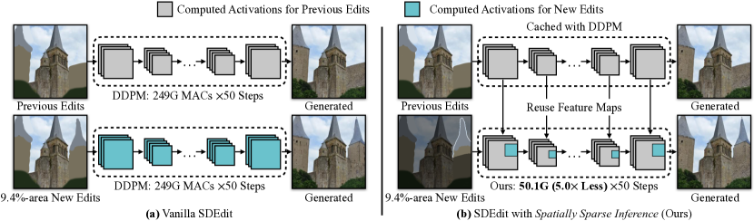
Figure 2: In the interactive editing scenario, a user adds a new building, which occupies 9.4% pixels. (a) Vanilla SDEdit has to apply denoising networks to the entire image, even though only a 9.4% area was edited. (b) Our method instead reuses the feature maps of the previous edits and only sparsely applies convolutions to the newly edited regions, which results in a $5.0\times$ MACs reduction for this example.

Deep generative models, such as GANs [6, 7] and diffusion models [8, 2, 1], excel at synthesizing photo-realistic images, enabling many image synthesis and editing applications. For example, users can edit an image by drawing sketches [9, 10], semantic maps [9, 4], or strokes [11]. All of these applications require users to interact with generative models frequently and therefore demand short inference time.

In practice, content creators often edit images gradually and only update a small image region each time. However, even for a minor edit, recent generative models often synthesize the entire image, including the unchanged areas, which leads to a significant waste of computation. As a concrete example shown in Figure 2(a), the result of the previous edits has already been computed, and the user further edits 9.4% areas. However, vanilla SDEdit [11] needs to apply the denoising network on the entire image to obtain the newly edited regions, wasting 80% computation on the unchanged areas. A naive approach to address this issue would be to first segment the newly edited regions, synthesize the corresponding output regions, and blend the outputs back into the previous output. Unfortunately, this method often creates visible seams between the newly edited and unedited regions. How could we save the computation by only updating the edited regions without losing global coherence?

In this work, we propose Spatially Sparse Inference (SSI), a general method to accelerate deep generative models, including conditional GANs and diffusion models, by utilizing the spatial sparsity of edited regions. Our method is motivated by the observation that feature maps in the unedited regions remain mostly the same during user editing. As shown in Figure 2(b), our key idea is to reuse the cached feature maps of the previous edits and sparsely update the newly edited areas. Specifically, given user input, we first compute a difference mask to locate the newly edited regions. For each convolution layer in the model, we only sparsely apply the filters to the masked regions while reusing the previous activations for the unchanged areas. The sparse update can significantly reduce the computation without hurting the image quality. However, the sparse update involves a gather-scatter process and often incurs significant latency overheads with existing deep learning frameworks. To address the issue, we propose Sparse Incremental Generative Engine (SIGE) to translate the theoretical computation reduction of our algorithm to measured latency reduction on various hardware.

To evaluate our method, we curate image editing and inpainting benchmarks on LSUN Church [12], Cityscapes [13] and LAION-5B [14]. Without loss of visual fidelity, we reduce the computation of DDPM [1, 2], Progressive Distillation [15], Stable Diffusion [3], and GauGAN [4] by up to $7.5\times$, $2.7\times$, $8.2\times$, and $18\times$, respectively, measured by MACs. Compared to existing generative model acceleration methods [5, 16, 17, 18, 19, 20, 21], our method directly uses the off-the-shelf pre-trained weights and could be applied to these methods as a plugin. When applied to GAN Compression [5], we reduce the computation of GauGAN by up $50\times$. See Figure 1 for some examples of our method. With SIGE, we accelerate DDPM by up to $3.0\times$ on NVIDIA RTX 3090, $4.6\times$ on Apple M1 Pro GPU, and $6.6\times$ on M1 Pro CPU, Stable Diffusion by up to $7.2\times$ on 3090, and GauGAN by up to $5.6\times$ on 3090, $5.2\times$ on M1 Pro GPU, and $14\times$ on M1 Pro CPU.

This journal paper extends our conference version [22] with new development and experiments in the following areas:

• We extend SIGE to support both self-attention and cross-attention layers by pruning unedited query tokens. This optimization can dramatically shrink the attention map size according to the edit size, reducing the computation and latency of the attention layers correspondingly.

• We further apply our method to Stable Diffusion [3], a widely-used text-to-image model with latency primarily bottlenecked by its self-attention layers. Since our previous engine can only accelerate convolutions, it can only reduce the computation by $1.6\times$ and latency by $1.1\times$ on Stable Diffusion, even with a $2.8\%$-area edit. In contrast, with our new attention optimization, we reduce Stable Diffusion’s computation and latency by $\sim 5\times$.

• We additionally support SIGE on the Metal Performance Shaders (MPS) backend to enable inference on the Apple M1 Pro GPU. On this hardware, we achieve up to $4.6\times$, $3.0\times$, and $5.2\times$ speedups for DDPM, Progressive Distillation, and GauGAN, respectively.

• We show additional results of SIGE with large and sequential edits. Specifically, on NVIDIA RTX 3090, our method remains faster than the original model with up to $\sim 70\%$ edits. For sequential edits, it can incrementally update the cached activations. We also include an extra ablation study regarding the dilation hyper-parameter to validate our design choice.

Our code, benchmarks and demo are available at https://github.com/lmxyy/sige.

2 Related Work

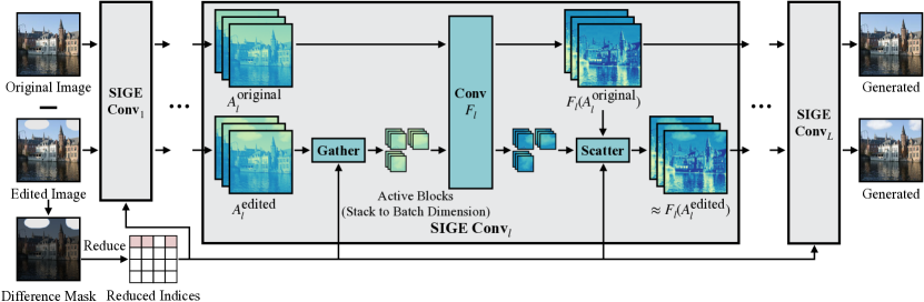
Figure 3: Tiling-based sparse convolution overview. For each convolution $F_{l}$ in the network, we wrap it into SIGE Conv_l. The activations of the original image are already pre-computed. When getting the edited image, we first compute a difference mask between the original and edited image and reduce the mask to the active block indices to locate the edited regions. In each SIGE Conv_l, we directly gather the active blocks from the edited activation $A^{\text{edited}}_{l}$ according to the reduced indices, stack the blocks along the batch dimension, and feed them into $F_{l}$. The gathered blocks have an overlap of width 2 if $F_{l}$ is $3\times 3$ convolution with stride 1 [23]. After getting the output blocks from $F_{l}$, we scatter them back into $F_{l}(A^{\text{original}}_{l})$ to get the edited output, which approximates $F_{l}(A^{\text{edited}}_{l})$.

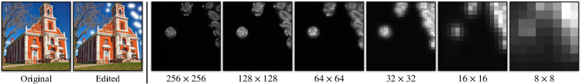
Figure 4: Left: Detailed edit example. Right: Channel-wise average of $|\Delta A_{l}|$ at the $l$-th layer of DDPM with different feature map resolutions. $|\Delta A_{l}|$ is sparse and non-zero values are aggregated at the edited regions.

Generative models. Generative models such as GANs [6, 7, 24, 25], diffusion models [2, 8, 26, 3], and auto-regressive models [27, 28] have demonstrated impressive photorealistic synthesis capability. They have also been extended to conditional image synthesis tasks such as image-to-image translation [29, 9, 30, 31], controllable image generation [11, 32, 4], and real image editing [33, 32, 34, 35, 36, 37, 38, 31]. Unfortunately, recent generative models have become increasingly computationally intensive, compared to their recognition counterparts. For example, GauGAN [4] consumes 281GMACs, 500$\times$ more than MobileNet [39, 40, 41]. Similarly, one key limitation of diffusion models [2] is their substantial computation cost and long inference time. To generate one image, DDPM requires hundreds or thousands of forwarding steps [2, 26], which is often infeasible in real-world interactive settings. To improve the sampling efficiency of DDPMs, recent works [1, 42, 43] propose to interpret the sampling process of DDPMs from the perspective of ordinary differential equations. However, these approaches still require hundreds of steps to generate high-quality samples. To further reduce the sampling cost, DDGAN [44] uses a multimodal conditional GAN to model each denoising step. Salimans et al. [15] propose to progressively distill a pre-trained DDPM model into a new one that requires fewer steps. Although this approach drastically reduces the sampling steps, the distilled model itself remains computationally prohibitive. Unlike prior work, our work focuses on reducing the computation cost of a pre-trained model. It is complementary to recent efforts on model compression, distillation, and the sampling step reduction of the diffusion models.

Model acceleration. People apply model compression techniques, including pruning [45, 46, 47, 48, 49, 50] and quantization [45, 51, 52, 53, 54, 55], to reduce the computation and model size of off-the-shelf deep learning models. Recent works apply Neural Architecture Search (NAS) [56, 57, 58, 59, 60, 61, 62] to automatically design efficient neural architectures. The above ideas can be successfully applied to accelerate the inference of GANs [5, 63, 64, 65, 16, 66, 17, 18, 19, 20, 21, 67]. Although these methods have achieved prominent compression and speedup ratios, they all reduce the computation from the model dimension but fail to exploit the redundancy in the spatial dimension during image editing. Besides, these methods require re-training the compressed model to maintain performance, while our method can be directly applied to existing pre-trained models. We show that our method can be combined with model compression [5] to achieve a $\sim 50\times$ MACs reduction in Section 4.2.

Sparse computation. Sparse computation has been widely explored in the weight domain [68, 69, 70, 71], input domain [72, 73], and activation domain [23, 74, 75, 76]. For activation sparsity, RRN [77] utilizes the sparsity in the consecutive video frame difference to accelerate video models. However, their sparsity is unstructured, which requires special hardware to reach its full speedup potential. Several works instead use structured sparsity. Li et al. [78] use a deep layer cascade to apply more convolution layers on the hard regions than the easy regions to improve the accuracy and speed of semantic segmentation. To accelerate 3D object detection, SBNet [23] uses a spatial mask, either from priori problem knowledge or an auxiliary network, to sparsify the activations. It adopts a tiling-based sparse convolution algorithm to handle spatial sparsity. Recent works further integrate the spatial mask generation network into the sparse inference network in an end-to-end manner [79] and extend the idea to different tasks [80, 81, 82, 83]. Compared to SBNet [23], our mask is directly derived from the difference between the original image and the edited image. Additionally, our method does not require any auxiliary network or extra model training. We also introduce other optimizations, such as normalization removal, kernel fusions and attention query pruning, to better adapt our engine for image editing.

3 Method

We build our method based on the following observation: during interactive image editing, a user often only changes the image content gradually. As a result, only a small subset of pixels in a local region is being updated at any moment. Therefore, we can reuse the activations of the original image for the unedited regions. As shown in Figure 3, we first pre-compute all activations of the original input image. During the editing process, we locate the edited regions by computing a difference mask between the original and edited image. We then reuse the pre-computed activations for the unedited areas and only update the edited regions by applying convolutional filters to them. In Section 3.1, we show the sparsity in the intermediate activations and present our main algorithm. In Section 3.2, we discuss the technical details of how our Sparse Incremental Generative Engine (SIGE) supports the sparse inference and converts the theoretical computation reduction to measured speedup on hardware.

3.1 Activation Sparsity

Preliminary. First, we closely study the computation within a single layer. We denote $A^{\text{original}}_{l}$ and $A^{\text{edited}}_{l}$ as the input tensor of the original image and edited image to the $l$-th convolution layer $F_{l}$, respectively. $W_{l}$ and $b_{l}$ are the weight and bias of $F_{l}$. The output of $F_{l}$ with input $A^{\text{edited}}_{l}$ could be computed in the following way due to the linearity of convolution:

$$F_{l}(A^{\text{edited}}_{l}) =W_{l}*A^{\text{edited}}_{l}+b_{l}$$

$$=W_{l}*(A^{\text{edited}}_{l}-A^{\text{original}}_{l})+(W_{l}*A^{\text{original}}_{l}+b_{l})$$

$$=W_{l}*\underbrace{\Delta A_{l}}_{\text{sparse}}+\underbrace{F_{l}(A^{\text{original}}_{l})}_{\text{pre-computed}},$$

where $*$ is the convolution operator and $\Delta A_{l}=A^{\text{edited}}_{l}-A^{\text{original}}_{l}$. If we have already pre-computed all the $F_{l}(A^{\text{original}}_{l})$, we only need to compute $W_{l}*\Delta A_{l}$. Naïvely, computing $W_{l}*\Delta A_{l}$ has the same complexity as $W_{l}*A^{\text{edited}}_{l}$. However, since the edited image shares similar features with the original image given a small edit, $\Delta A_{l}$ should be sparse. Below, we discuss different strategies to leverage the activation sparsity to accelerate model inference.

Our first attempt was to prune $\Delta A_{l}$ by zeroing out elements smaller than a certain threshold to achieve the target sparsity. Unfortunately, this pruning method fails to achieve measured speedup due to the overheads of the on-the-fly pruning and irregular sparsity pattern.

Structured sparsity. Fortunately, user edits are often highly structured and localized. As a result, $\Delta A_{l}$ should also share the structured spatial sparsity, where non-zero values are mostly aggregated within the edited regions, as shown in Figure 4. We then directly use the original and edited images to compute a difference mask and sparsify $\Delta A_{l}$ with this mask.

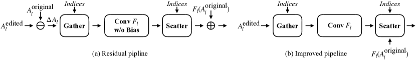
Figure 5: Titling-based sparse convolution pipelines. (a) We first compute the activation difference $\Delta A_{l}$ and gather the active blocks along the batch dimension from it according to the indices reduced from the difference mask. We then feed the blocks into the convolution $F_{l}$ without bias, scatter the output into a zero tensor, and add the residual $F_{l}(A^{\text{original}}_{l})$ back. (b) We directly gather the blocks from $A^{\text{edited}}_{l}$ without computing $\Delta A_{l}$. $F_{l}$ is computed with bias. We scatter the output into $F_{l}(A^{\text{original}}_{l})$ instead of a zero tensor.

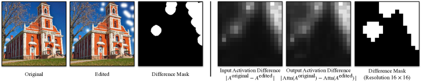
Figure 6: The input and output activation differences of a $16\times 16$ self-attention layer in the DDPM model. Left: Detailed edit example with the difference mask. Right: Activation differences with the downsampled difference mask. Attn is the self-attention layer. Brighter colors refer to larger differences. Both the input and output differences match the mask well.

3.2 Sparse Engine SIGE

But how could we leverage the structured sparsity to accelerate $W_{l}*\Delta A_{l}$? A naïve approach is to crop a rectangular edited region out of $\Delta A_{l}$ for each convolution and only compute features for the cropped regions. Unfortunately, this naïve cropping method works poorly for the irregular edited regions (e.g., the example shown in Figure 4).

Tiling-based sparse convolution. Instead, as shown in Figure 5(a), we use a tiling-based sparse convolution algorithm. We first downsample the difference mask to different scales and dilate the downsampled masks (width 1 for diffusion models and 2 for GauGAN). Then we divide $\Delta A_{l}$ into multiple small blocks of the same size spatially and index the difference mask at the corresponding resolution. Each block index refers to a single block with non-zero elements. We then gather the non-zero blocks (i.e., active blocks) along the batch dimension and feed them into the convolution $F_{l}$. Finally, we scatter the output blocks into a zero tensor according to the indices to recover the original spatial size and add the pre-computed residual $F_{l}(A^{\text{original}}_{l})$ back. The gathered active blocks overlap with width 2 for $3\times 3$ convolution with stride 1 to ensure the output blocks of the adjacent input blocks are seamlessly stitched together [23].

This pipeline in Figure 5(a) is equivalent to a simpler pipeline in Figure 5(b). Instead of gathering $\Delta A_{l}$, we could directly gather $A^{\text{edited}}_{l}$. The convolution needs to be computed with bias $b_{l}$. Besides, we need to scatter the output blocks into $F_{l}(A^{\text{original}}_{l})$ instead of a zero tensor. Thus, we do not need to store $A^{\text{original}}_{l}$ anymore, which further saves memory and removes the overheads of addition and subtraction. Figure 3 visualizes the pipeline.

However, the aforementioned pipeline still fails to produce a noticeable speedup due to extra kernel calls and memory movement overheads in Gather and Scatter. For example, the original dense $3\times 3$ convolution with 128 channels and input resolution $256\times 256$ takes 0.78ms on NVIDIA RTX 3090. The sparse convolution using pipeline Figure 5(b) on the example shown in Figure 4 (15.5% edited regions) still needs 0.42ms in total, with the Gather and Scatter operations accounting for a significant overhead of 0.17ms (41%). To mitigate these overheads, we further optimize SIGE by pre-computing normalization parameters and applying kernel fusion. Additionally, we extend SIGE to support attention layers.

Pre-computing normalization parameters. For batch normalization [84], it is easy to remove the normalization layer during inference time since we can use pre-computed mean and variance statistics from model training. However, recent generative models often use instance normalization [85, 86] or group normalization [87, 88], which compute the statistics on the fly during inference. These normalization layers incur overheads as we need to estimate the statistics from the full-size tensors. However, as the original and edited images are quite similar given a small user edit, we assume $A^{\text{original}}_{l}\approx A^{\text{edited}}_{l}$. This allows us to reuse the statistics of $A^{\text{original}}_{l}$ for the normalization instead of recomputing them for $A^{\text{edited}}_{l}$. Thus, normalization layers could be replaced by simple Scale+Shift operations with pre-computed $A^{\text{original}}_{l}$ statistics.

Kernel fusion. As mentioned before, both the Gather and Scatter operations introduce significant data movement overheads. To reduce it, we fuse several element-wise operations (Scale+Shift and Nonlinearity) into Gather and Scatter [23, 89, 90] and only apply these element-wise operations to the active blocks (i.e., edited regions). Furthermore, we perform the in-place computation to reduce the number of kernel calls and memory allocation overheads.

In Scatter, we need to copy the pre-computed activation $F_{l}(A^{\text{original}}_{l})$. This copying operation is highly redundant, as most elements from $F_{l}(A^{\text{original}}_{l})$ do not involve any computation given a small edit and will be discarded in the next Gather. To reduce the tensor copying overheads, we fuse the Scatter with the following Gather by directly gathering the active blocks from $F_{l}(A^{\text{original}}_{l})$ and the input blocks to be scattered. Sometimes, the residual connection in the ResBlock [91] contains a shortcut $1\times 1$ convolution to match the channel number of the residual and the ResBlock output. We also fuse the Scatter in the shortcut branch, main branch, and the residual addition together to avoid the tensor copying overheads in the shortcut Scatter. Please refer to Appendix A for more details.

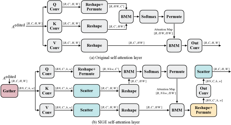
Figure 7: The original self-attention layer vs. SIGE self-attention layer. All convolutions are $1\times 1$, with batch size $B$, and the number of input and hidden channels $C$ and $C^{\prime}$, respectively. The height and width of the input are represented by $H$ and $W$. $N$ denotes the number of active blocks, and $h$ and $w$ denote the height and width of the active blocks. For simplicity, we omit the original activation and active indices input to Gather and Scatter. The original pipeline computes the attention map for all query tokens. Our SIGE pipeline instead first gathers the active blocks and feeds them to the Q, K, and V convolutions. Then, only the keys and values are scattered back. Thus, only the edited query tokens are preserved, so the attention map size is reduced. After the Out Conv, the result tensor is scattered back into the original activation to obtain the final output.

Extension to attention layers. Recent models have adopted attention layers to enhance the image quality [92, 93] and controllability [3]. These attention layers could model long-range dependencies across image regions, potentially introducing non-local changes. However, when the edited region is small, it only has limited impacts on the unedited areas. Figure 6 illustrates the difference maps for both the input and output activations of a $16\times 16$ self-attention layer in the DDPM model, both of which closely match the difference mask. This indicates that user edits often change activations locally, even with attention layers, and our method’s assumption still holds.

Based on this observation, we extend SIGE to attention layers. Figure 7 illustrates the difference between the vanilla and SIGE self-attention layer. As the unedited regions remain mostly unchanged, there is no need to compute the attention map for these areas. In our pipeline, Gather selectively prunes the unedited regions, only preserving the edited ones. After the Q, K, and V convolutions, we only scatter the keys and values back into the original activations. Thus, the query token number is reduced according to the edit ratio, and more importantly, it also reduces the size of the attention map correspondingly. Such memory reduction can lead to almost linear speedup even on an NVIDIA RTX 3090 GPU, as shown in Figure 1 and Figure 9.

4 Experiments

Model	Method	MACs		PSNR ($\uparrow$)		LPIPS ($\downarrow$)		FID ($\downarrow$)	mIoU ($\uparrow$)
		Value	Ratio	with G.T.	with Orig.	with G.T.	with Orig.
DDPM	Original	249G	–	26.8	–	0.069	–	65.4	–
	40% Pruning	–	–	24.9	31.0	0.991	0.101	72.2	–
	Patch	72.0G	3.5$\times$	26.8	40.6	0.076	0.022	66.4	–
	Ours	65.3G	3.8$\times$	26.8	52.4	0.070	0.009	65.8	–
	Original	66.9G	–	21.9	–	0.143	–	90.0	–
PD	40% Pruning	–	–	21.6	37.6	0.164	0.051	101	–
	Ours	32.5G	2.1$\times$	21.9	60.7	0.154	0.003	90.1	–
GauGAN	Original	281G	–	15.8	–	0.409	–	55.4	62.4
	GAN Comp. [5]	31.2G	9.0$\times$	15.8	19.5	0.412	0.288	55.5	61.5
	Ours	30.7G	9.2$\times$	15.8	26.5	0.413	0.113	54.4	62.1
	0.19 GauGAN	13.3G	21$\times$	15.5	18.6	0.424	0.322	57.9	53.5
	GAN Comp. (S)	9.64G	29$\times$	15.7	19.1	0.422	0.310	50.4	57.4
	GAN Comp.+Ours	7.06G	40$\times$	15.7	19.2	0.416	0.299	54.6	60.0
	Original	805G	–	19.3	–	0.153	–	27.2	–
Stable Diffusion	50% Pruning	–	–	20.5	20.7	0.172	0.149	36.6	–
	Ours	387G	2.1$\times$	19.2	19.9	0.157	0.126	26.8	–

TABLE I: Quantitative evaluation. MACs measures the average computation for a single model forward over the entire dataset. PSNR/LPIPS with G.T. means computing the metrics with the ground-truth images, and with Orig. means computing with the generated samples from the original model. $P\%$ Pruning: Uniformly pruning $P\%$ model weights without fine-tuning. Patch: Cropping the smallest image patch that covers all the edited regions and blending the output patch into the original image. 0.19 GauGAN: Uniformly reducing each layer of GauGAN to 19% channels and training from scratch. GAN Comp. (S): GAN Compression with a larger compression ratio. For all models, our method outperforms other baselines with less computation.

Below we first describe our experiment setups, including models, baselines, datasets, and evaluation protocols. We then discuss our main qualitative and quantitative results. Finally, we include a detailed ablation study regarding the importance of each algorithmic design.

4.1 Setups

Models. We conduct experiments on the following four models, including diffusion models and GAN-based models, to explore the generality of our method.

• DDPM [2] is a diffusion probabilistic model that models the data distribution through an iterative denoising process. It adopts a U-Net [94] backbone for the denoising network. For fast sampling, we use DDIM [1] sampler to reduce the number of denosing steps from 1000 to 100.

• Progressive Distillation (PD) [15] adopts network distillation [95] to progressively reduce the number of steps for diffusion models.

• Stable Diffusion (SD) [3] is a text-to-image latent diffusion model [3]. It uses a VAEGAN-based autoencoder to compress the image to a compact latent and applies the diffusion model in the latent space. The model includes multiple cross-attention layers to support text conditioning.

• GauGAN [4] is a paired image-to-image translation model which learns to generate a high-fidelity image given a semantic label map.

Baselines. We compare our methods against the following baselines:

• Patch. We crop the smallest patch covering all the edited regions, feed it into the model, and blend the output patch into the original image.

• Crop. For each convolution $F_{l}$, we crop the smallest rectangular region that covers all masked elements of the activation $A^{\text{edited}}_{l}$, feed it into $F_{l}$, and scatter the output patch into $F_{l}(A^{\text{original}}_{l})$.

• $P\%$ Pruning. We uniformly prune $P\%$ model weights without further fine-tuning. This is fair as our method uses pre-trained weights without fine-tuning. Since the fine-grained pruning is unstructured, it requires special hardware to achieve measured speedup, so we do not report MACs for this baseline.

• 0.19 GauGAN. We reduce each convolution layer of GauGAN to $19\%$ channels ($21\times$ MACs reduction) and train it from scratch.

• GAN Compression [5]. A general-purpose compression method for conditional GANs. GAN Comp. (S) means GAN Compression with a larger compression ratio.

• 0.5 Original means linearly scaling each layer of the original model to 50% channels, and we only use this to benchmark our efficiency results.

Datasets. We use the following three datasets:

• LSUN Church. We use the LSUN Church Outdoor dataset [12] and follow the same preprocessing steps as prior works [2, 42]. To automatically generate a stroke editing benchmark, we first use Detic [96] to segment the images in the validation set. For each segmented object, we use its segmentation mask to inpaint the image by CoModGAN [97] and treat the inpainted image as the original image. We generate the corresponding user strokes by first blurring the masked regions with the median filter and quantizing it into 6 colors following SDEdit [11]. We collect 454 editing pairs in total (431 synthetic + 23 manual). We evaluate DDPM [2, 1] and PD [15] on this dataset.

• Cityscapes. The dataset [13] contains images of German street scenes. The training and validation sets consist of 2,975 and 500 images, respectively. Our editing dataset has 1,505 editing pairs in total. We evaluate GauGAN [4] on this dataset.

• LAION. We select a random subset of 1,000 images from LAION-5B [14] that meet or exceed $1024\times 1024$ resolution. These images are then center-cropped and resized to $512\times 512$ resolution. Next, we randomly occlude between $1\%$ and $25\%$ of the image area using circular masks. We use Stable Diffusion [3] to inpaint the region and evaluate the visual quality of the output.

Please refer to Appendix B for more details about the benchmark datasets.

Metrics. Following previous works [11, 5, 4], we use the standard metrics Peak Signal Noise Ratio (PSNR, higher is better), LPIPS (lower is better) [98], and Fréchet Inception Distance (FID, lower is better) [99, 100] to evaluate the image quality. For Cityscapes, we additionally adopt a semantic segmentation metric to evaluate the generated images. Specifically, we run DRN-D-105 [101] on the generated images and compute the mean Intersection over Union (mIoU) of the segmentation results. Generally, a higher mIOU indicates that the generated images look more realistic and better align with the input.

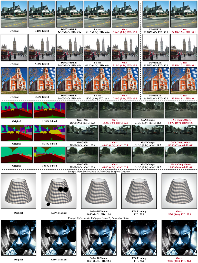
Figure 8: Qualitative results of our method under different edit or mask sizes. MACs measure the computation for a single model forward. Our method well preserves the visual fidelity of the original model without losing global context. On the contrary, Patch (cropping the smallest image patch that covers all the edited regions and scattering the output patch back into the original image) performs poorly because of the lack of global context when the edit is small.

Implementation details. We use DDIM sampler [1] for both DDPM and Stable Diffusion (SD). Specifically, the number of total denoising steps for DDPM, SD, and Progressive Distillation (PD) are 100, 50, and 8, respectively, and we use 50, 40, and 5 steps for SDEdit [11]. We dilate the difference mask by 5, 5, 2, 5, and 1 pixels for DDPM, SD, PD with resolution 128, PD with resolution 256, and GauGAN, respectively. For SD decoder, we dilate the difference mask by 45 pixels. Besides, we apply SIGE to all convolutional layers whose input feature map resolutions are larger than $32\times 32$, $16\times 16$, $8\times 16$ and $16\times 32$ for DDPM, PD, original GauGAN, and GAN Compression, respectively. For SD, we apply SIGE to all convolutional layers and attention layers except ones in the middle stages. As the attention layers in DDPM and PD only consume a small portion of the overall latency, we do not apply SIGE to them. For diffusion models, we pre-compute and reuse the statistics of the original image for all group normalization layers [87]. For GANs, we pre-compute and reuse the statistics of the original image for all instance normalization layers [85] whose resolution is higher than $16\times 32$. For all models, the sparse block size for $3\times 3$ convolution is 6, and $1\times 1$ convolution is 4. All results are measured with FP32 precision.

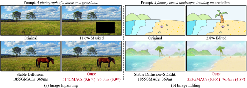
Figure 9: Qualitative results of Stable Diffusion [3]. The computation and latency are measured for a single diffusion step on NVIDIA RTX 3090. For image inpainting, with $11.6\%$ masked regions, our method reduces the computation by $3.6\times$, resulting in a $3.9\times$ speedup. For image editing, we reduce the computation by $5.3\times$, achieving a $4.8\times$ speedup with a $2.8\%$-area edit.

Model

Edit Size

Method

MACs

3090

2080Ti

Intel Core i9

M1 Pro CPU

M1 Pro GPU

Value

Ratio

Value

Ratio

Value

Ratio

Value

Ratio

Value

Ratio

Value

Ratio

DDPM

–

Original

248G

–

37.5ms

–

54.6ms

–

609ms

–

12.9s

–

183ms

–

0.5 Original

62.5G

4.0$\times$

20.0ms

1.9$\times$

31.2ms

1.8$\times$

215ms

2.8$\times$

3.22s

4.0$\times$

90.5ms

2.0$\times$

1.20%

Crop

32.6G

7.6$\times$

15.5ms

2.4$\times$

29.3ms

1.9$\times$

185ms

3.3$\times$

1.85s

6.9$\times$

52.1ms

3.5$\times$

Ours

33.4G

7.5$\times$

12.6ms

3.0$\times$

19.1ms

2.9$\times$

147ms

4.1$\times$

1.96s

6.6$\times$

39.5ms

4.6$\times$

15.5%

Crop

155G

1.6$\times$

30.5ms

1.2$\times$

44.5ms

1.2$\times$

441ms

1.4$\times$

8.09s

1.6$\times$

144ms

1.3$\times$

Ours

78.9G

3.2$\times$

19.4ms

1.9$\times$

29.8ms

1.8$\times$

304ms

2.0$\times$

5.04s

2.6$\times$

75.8ms

2.4$\times$

PD256

–

Original

119G

–

35.1ms

–

51.2ms

–

388ms

–

6.18s

–

178ms

–

0.5 Original

31.0G

3.8$\times$

29.4ms

1.2$\times$

43.2ms

1.2$\times$

186ms

2.1$\times$

1.72s

3.6$\times$

151ms

1.2$\times$

1.20%

Ours

25.9G

4.6$\times$

18.6ms

1.9$\times$

26.4ms

1.9$\times$

152ms

2.5$\times$

1.55s

4.0$\times$

59.9ms

3.0$\times$

15.5%

Ours

48.5G

2.5$\times$

21.4ms

1.6$\times$

30.7ms

1.7$\times$

250ms

1.6$\times$

3.22s

1.9$\times$

73.3ms

2.4$\times$

GauGAN

–

Original

281G

–

45.4ms

–

49.5ms

–

682ms

–

14.1s

–

151ms

–

GAN Compression

31.2G

9.0$\times$

15.1ms

3.0$\times$

25.0ms

2.0$\times$

333ms

2.1$\times$

2.11s

6.7$\times$

75.3ms

2.0$\times$

1.18%

Ours

15.3G

18$\times$

8.11ms

5.6$\times$

19.3ms

2.6$\times$

114ms

6.0$\times$

0.990s

14$\times$

29.1ms

5.2$\times$

GAN Comp.+Ours

5.59G

50$\times$

8.72ms

5.2$\times$

16.2ms

3.1$\times$

53.1ms

13$\times$

0.370s

38$\times$

25.6ms

5.9$\times$

13.5%

Ours

69.8G

4.0$\times$

17.8ms

2.5$\times$

27.1ms

1.8$\times$

238ms

2.9$\times$

4.06s

3.5$\times$

89.1ms

1.7$\times$

GAN Comp.+Ours

10.8G

26$\times$

10.0ms

4.5$\times$

17.4ms

2.8$\times$

94.4ms

7.2$\times$

0.741s

19$\times$

45.5ms

3.3$\times$

–

Original

1855G

–

369ms

–

–

–

8.93s

–

–

–

–

–

Stable

0.5 Original

593G

3.1$\times$

279ms

1.3$\times$

–

–

6.79s

1.3$\times$

–

–

–

–

Diffusion

2.78$\%$

Ours

353G

5.3$\times$

76.4ms

4.8$\times$

–

–

1.37s

6.5$\times$

–

–

–

–

11.5$\%$

Ours

514G

3.6$\times$

95.0ms

3.9$\times$

–

–

2.35s

3.5$\times$

–

–

–

–

TABLE II: Measured computation and latency for a single model forward on different devices. The detailed edit examples are shown in Figure 8 and 9. 0.5 Original: Linearly scaling each layer of the model to 50% channels. Crop: For each convolution, we find the smallest patch covering the masked elements, crop it out, feed it into the convolution and scatter the output patch into the original image activation. Our method could reduce up to 18$\times$ MACs and achieve up to 5.6$\times$, $2.9\times$, 6.0$\times$, 14$\times$, and $5.2\times$ latency reductions on NVIDIA RTX 3090, 2080Ti, Intel Core i9-10920X and M1 Pro CPU and GPU. With GAN Compression, we could further speed up GauGAN by $9.5\times$ on Intel Core-i9 and $38\times$ on Apple M1 Pro CPU.

4.2 Main Results

Image quality. We report the quantitative results of applying our method to DDPM [2, 1], PD [15], GauGAN [4], and Stable Diffusion [3] on SDEdit [11] image editing and text-guided inpainting in Table I. Figure 8 shows some qualitative results. For PSNR and LPIPS, with G.T. means computing the metric with the ground-truth images. With Orig. means computing the metric with the samples generated by the original model. On LSUN Church, we only use 431 synthetic images for the PSNR/LPIPS with G.T. metrics, as manual edits do not have ground truths. For the other metrics, we use the entire LSUN Chur ch dataset (431 synthetic + 23 manual edits). On Cityscapes, we view the synthetic semantic maps as the original input and the ground-truth semantic maps as the edited input for the PSNR/LPIPS with G.T. metrics, which has 1505 samples. For the other metrics, we include the symmetric edits (view the ground-truth semantic maps as the original inputs and synthetic semantic maps as the edited inputs), with 3010 samples in total. For the models with method Patch and Ours, whose computation is edit-dependent, we measure the average MACs over the whole dataset.

For SDEdit with DDPM and PD, our method outperforms all baselines consistently and achieves results on par with the original model. The Patch inference fails when the edited region is small as the global context is insufficient. Although our method only applies convolutional filters to the local edited regions, it can reuse the global context stored in the original activations. Therefore, it performs the same as the original model. For GauGAN, our method also performs better than GAN Compression [5] with an even larger MACs reduction. When applying it to GAN Compression, we further achieve a $\sim 40\times$ MACs reduction with minor performance degradation, beating both 0.19 GauGAN and GAN Comp. (S). For Stable Diffusion, SIGE reduces its computation by $2.1\times$ on average while maintaining LPIPS [98] and FID [99, 100]. As illustrated in Figure 8, although 50% Pruning achieves higher PSNR values, it significantly lags in visual quality compared to both the original model and our method. In addition to the automatically generated inpainting examples, we manually curate two $512\times 1024$ examples on image inpainting and image-to-image translation in Figure 9. Our method closely mirrors the original model’s results while reducing the cost by $4\sim 5\times$.

Model efficiency. For real-world interactive image editing applications, inference acceleration on hardware is more critical than computation reduction. To verify the effectiveness of our proposed engine, we measure the speedup of the edit examples shown in Figure 8 for DDPM, PD and GauGAN and 9 for Stable Diffusion on five devices, including NVIDIA RTX 3090, NVIDIA RTX 2080Ti, Intel Core i9-10920X CPU, and Apple M1 Pro CPU and GPU, with different computational powers. We use batch size 1 to simulate real-world use. For GPU devices, we first perform 200 warm-up runs and measure the average latency of the next 200 runs. For CPU devices, we perform 10 warm-up runs and 10 test runs, repeat this process 5 times and report the average latency. The results are shown in Table II.

The original Progressive Distillation [15] can only generate $128\times 128$ images, which is too small for real use. We add some extra layers to adapt the model to resolution $256\times 256$. For the Crop baseline, we also pre-compute the normalization parameters for fair comparisons. When the edit pattern is like a rectangle, this baseline reduces similar computation with ours (e.g., the first example of DDPM in Figure 8). However, the speedup is still worse than ours on various devices due to the large memory index overheads in native PyTorch. When the edited region is far from a rectangle (e.g., the third example of DDPM), the cropped patch has much redundancy. Therefore, even though only 15.5% areas are edited, the MACs reduction is only 1.6$\times$. For Stable Diffusion, as mentioned in Section 7, by selectively pruning unedited queries, SIGE reduces the attention map size and memory overheads in attention layers. For $512\times 1024$ image editing example in Figure 9, the first self-attention layer of the diffusion network takes $64\times 128$ input, resulting in an $8192\times 8192$ attention map. SIGE reduces the attention map size to $672\times 8192$ ($12\times$ smaller). Therefore, it can achieve a similar speedup ratio to the computation reduction even on GPUs. SIGE achieves up to 5.6$\times$, 2.9$\times$, 6.0$\times$, 14$\times$, and 5.2$\times$ speedups on RTX 3090, 2080Ti, Intel Core i9-10920X, Apple M1 Pro CPU and GPU, respectively. When applied to GAN Compression, SIGE achieves 9.5$\times$ and 38$\times$ latency reductions on Intel Core i9 and Apple M1 Pro CPU, respectively. Additionally, we apply SIGE to the encoder and decoder part of Stable Diffusion. For the image editing example in Figure 9, this results in an $8\times$ speedup for the encoder and a $5\times$ speedup for the decoder.

Large edits. In Figure 10, we further analyze the DDPM’s and GauGAN’s computation/latency vs. edit ratio curves on both NVIDIA RTX 3090 and Intel Core i9. On both devices, computation and latency scale linearly with the edit ratio. For the RTX 3090, our method delivers speed improvements up to edit ratios between $65\%$ and $75\%$. On the Intel Core i9, the ceiling is approximately $45\%$. Figure 11 showcases examples with large edit ratios exceeding $50\%$, where SIGE still matches the original model in visual quality. Moreover, in real-world applications, users can break down large edits into smaller increments. Our method facilitates fast updates as these incremental edits are applied, as discussed below.

Sequential edits. In Figure 12, we show the results of sequential edits with our method. Specifically, One-time Pre-computation performs as well as the Full Model, demonstrating that our method can be applied to multiple sequential edits with only one-time pre-computation in most cases. Moreover, for extremely large edits, we could use SIGE to incrementally update the pre-computed features (Incremental Pre-computation) and condition the later edits on the recomputed one. Its results are also as good as the full model.

4.3 Ablation Study

Below we perform several ablation studies to show the effectiveness of each design choice.

Memory usage. The pre-computed activations of the original image require additional memory storage. We profile the peak memory usage of the original model and our method in PyTorch. Our method only increases the peak memory usage of a single forward for DDPM [2], PD [15], GauGAN [4], and GAN Compression [5] by 0.1G, 0.1G, 0.8G, and 0.3G, respectively with FP32 precision. Specifically, it needs to store additional 169M, 56M, 239M, 275M, and 120M parameters for DDPM, PD, Stable Diffusion [3], original GauGAN and GAN Compression, respectively, for a single forward. For the diffusion models, we need to store activations for all iteration steps (e.g., 50 for DDIM sampler [1] and 5 for PD). However, data movement and kernel computation are asynchronous on GPU, so we could store the activations in CPU memory and load the on-demand ones on GPU to reduce peak memory usage.

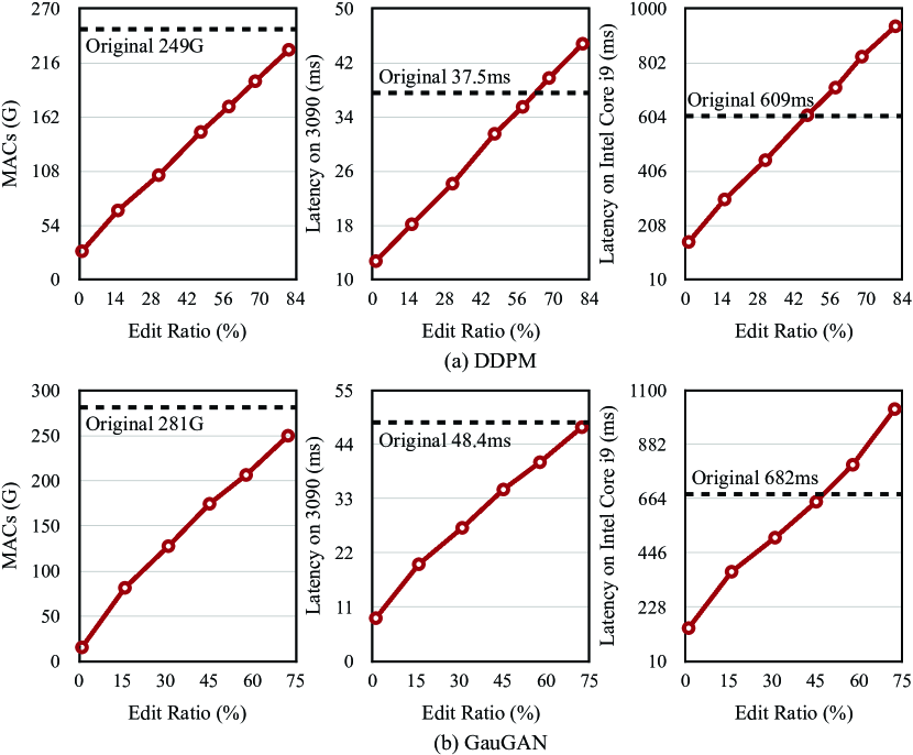
Figure 10: Computation/latency vs. edit ratio curves of SIGE for DDPM and GauGAN. The black dashed line represents the performance of the original model. Both computation and latency scale linearly with the edit ratio. On NVIDIA RTX 3090, our method attains speedups for edits up to $75\%$, and on Intel Core i9, up to $45\%$.

Figure 11: Qualitative results of SIGE with large edits. With $50\sim 60\%$ edits, SIGE can still preserve visual fidelity of the original model without losing global context while reducing the computation by up to $1.5\times$.

Figure 12: Sequential editing results with SIGE. The computation and latency are measured on NVIDIA RTX 3090 for a single forward. Full Model means the results with the full model. One-time Pre-computation means we pre-compute the original image features for all the edit steps. Incremental Pre-computation means we incrementally update the pre-computed features with SIGE before the next edit step. The image quality of all methods is quite similar.

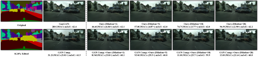
Figure 13: Visualization results of different dilation sizes on GauGAN. Although without mIoU improvement, increasing the dilation could smoothly blend the boundary between the edited region and unedited regions to improve the image quality slightly. Specifically, the shadow boundary of the added car fades when dilation increases. However, it will incur more computations.

Speedup of each design. Table III shows the effectiveness of each optimization we add to SIGE. For DDPM on RTX 2080Ti, naïvely applying the tiling-based sparse convolution can reduce the computation by 7.6$\times$. Still, the latency reduction is only 1.6$\times$ due to the large memory overheads in Gather and Scatter. Pre-computing the normalization parameters can remove the latency of normalization statistics calculation and reduce the overall latency to 29.6ms. Fusing element-wise operations into the Gather and Scatter can remove redundant operations in the unedited regions and also reduce the memory allocation overheads (about 9ms). Finally, fusing the Scatter and Gather to Scatter-Gather and Scatter in the shortcut branch and main branch can further reduce about 1.6ms tensor copying overheads, achieving a 2.9$\times$ speedup. For Stable Diffusion [3] on RTX 3090, both the computation reduction ($1.6\times$) and the speedup ($1.1\times$) are poor without our SIGE attention, as the large attention map incurs significant memory overheads. With our SIGE attention, we achieve a $5.3\times$ MACs reduction. Moreover, as we prune the unedited query tokens to reduce the attention map size accordingly, the memory overheads decrease correspondingly. Therefore, the speedup is much more prominent (4.8$\times$).

Experiments with TensorRT. Real-world model deployment also depends on deep learning backends with optimized libraries and runtimes. To demonstrate the effectiveness and extensibility of SIGE, we also implement our kernels in a widely-used backend TensorRT and benchmark the DDPM latency results on RTX 2080Ti in Table IV. Specifically, our speedup ratio becomes more prominent with TensorRT compared to PyTorch, especially for small edits, as TensorRT better supports small convolutional kernels with higher GPU utilization than PyTorch.

Dilation hyper-parameter. We show the results of our method with different dilation on GauGAN in Figure 13. Increasing the dilation incurs more computations but also slightly improves the image quality. Specifically, the shadow boundary of the added car fades as the dilation increases. We choose dilation 1 since the image quality is almost the same as 20 while delivering the best speed.

Models	MACs	Optimizations					Latency
		Sparse	Norm.	Elem.	Sct.	Attn.	Value	Ratio
	249G						54.6ms	–
		$\checkmark$					34.0ms	1.6$\times$
DDPM	32.6G	$\checkmark$	$\checkmark$				29.6ms	1.8$\times$
	(7.6$\times$)	$\checkmark$	$\checkmark$	$\checkmark$			20.7ms	2.6$\times$
		$\checkmark$	$\checkmark$	$\checkmark$	$\checkmark$		19.1ms	2.9$\times$
	1855G						369ms	–
SD	1193G (1.6$\times$)	$\checkmark$	$\checkmark$	$\checkmark$	$\checkmark$		335ms	1.1$\times$
	353G (5.3$\times$)	$\checkmark$	$\checkmark$	$\checkmark$	$\checkmark$	$\checkmark$	76.4ms	4.8$\times$

TABLE III: Ablation study of each optimization. Sparse: Using tiling-based sparse convolution. Norm.: Pre-computing normalization parameters. Elem.: Fusing element-wise operations. Sct.: Fusing Scatter to reduce the tensor copying overheads. Attn.: Using SIGE attention layers. With all optimizations, we could reduce the latency of DDPM by 2.9$\times$ on NVIDIA RTX 2080Ti and Stable Diffusion by 4.8$\times$ on RTX 3090.

Method	Edit Size	MACs		PyTorch		TensorRT
		Value	Ratio	Value	Ratio	Value	Ratio
Original	–	249G	–	54.6ms	–	47.7ms	–
	1.20%	33.4G	7.5$\times$	19.1ms	2.9$\times$	14.4ms	3.3$\times$
Ours	7.19%	51.8G	4.8$\times$	22.1ms	2.5$\times$	18.6ms	2.6$\times$
	15.5%	78.9G	3.2$\times$	29.8ms	1.8$\times$	26.9ms	1.8$\times$

TABLE IV: Latency comparisons of DDPM on RTX 2080Ti between PyTorch and TensorRT. The speedup ratio is larger in TensorRT than PyTorch, especially when the edit size is small.

5 Conclusion & Discussion

For image editing, existing deep generative models often waste computation by re-synthesizing the image regions that do not require modifications. To solve this issue, we have presented a general-purpose method, Spatially Sparse Inference (SSI), to selectively perform computation on edited regions, and Sparse Incremental Generative Engine (SIGE) to convert the computation reduction to latency reduction on commonly-used hardware. We have demonstrated the effectiveness of our approach in various hardware settings.

Limitations. As discussed in Section 4.3, our method requires extra memory to store the original activations, which slightly increases the peak GPU memory usage. It may not work on certain memory-constrained devices, especially for the diffusion models (e.g., DDPM [1]), since our method requires storing activations of all denoising steps. However, recent advancements of few-step samplers [1, 44, 102, 103, 104, 43, 105] and low-precision inference [106, 107] have lowered the memory threshold and make it possible to apply our method to diffusion models.

We assume the text input is fixed when applying SIGE to Stable Diffusion [3]. For text changes, our method requires recomputing the cached activations, potentially limiting its use cases. Besides, our current method cannot handle text-to-image generation, since even minor adjustments to the text can lead to significant global changes. We leave this as future work.

Our engine has limited speedup on convolutions with low resolution. When the input resolution is low, the active block size needs to be even smaller to get a decent sparsity, such as 1 or 2. However, such extremely small block sizes have bad memory locality and will result in low hardware efficiency.

Besides, we sometimes observe some noticeable boundaries between the edited regions and unedited regions in our generated samples of GauGAN [4]. This is because, for GauGAN model, the unedited regions also change slightly when we perform normal inference. However, since our method does not update the unedited region, there may be some visible seams between the edited and unedited areas, even though the semantics are coherent. Dilating the difference mask would help reduce the gap.

In most cases, the edit will only update the edited regions. However, sometimes the edit will also introduce global illumination changes such as shadow and reflection. For this case, as we only update the edited areas, we cannot update the global changes outside them accordingly.

Societal impact. In this paper, we investigate how to update user edits locally without losing global coherence to enable smoother interaction with the generative models. In real-world scenarios, people could use an interactive interface to edit an image, and our method could provide a quick and high-quality preview for their edits, which eases the process of visual content creation and reduces energy consumption, leading to a greener AI application. The reduced cost also provides a good user experience for lower-end devices, which further democratizes the applications of generative models.

However, our method can be utilized by malicious users to generate fake content, deceive people, and spread misinformation, which may lead to potential negative social impacts. Following previous works [11], we explicitly specify the usage permission of our engine with proper licenses. Additionally, we run a forensics detector [108] to detect the generated results of our method. On GauGAN, our generated images can be detected with $97.2\%$ average precision (AP). However, on DDPM [2, 1] and Progressive Distillation [15], the APs are only $56.6\%$ and $52.4\%$. Such low APs are caused by the model differences between GANs and diffusion models, as observed in SDEdit [11]. We believe developing forensic methods for diffusion models is a critical future research direction.

Appendix A Kernel Fusion

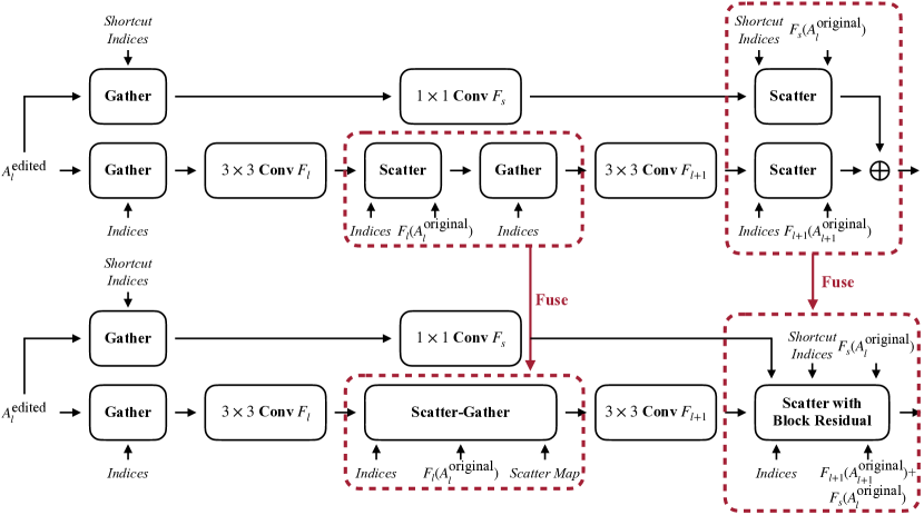
Figure 14: Visualization of kernel fusion in DDPM [1] ResBlock [91]. We omit the element-wise operations for simplicity and follow the notations in Section 3. As the kernel sizes of the convolution in the shortcut branch and main branch are different, their reduced active block indices are different (Indices and Shortcut Indices). To reduce the tensor copying overheads in Scatter, we fuse Scatter with the following Gather into Scatter-Gather and fuse the Scatter in the shortcut, main branch, and residual addition into Scatter with Block Residual. We pre-compute an additional Scatter Map for the Scatter-Gather kernel.

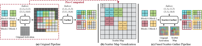
Figure 15: Scatter-Gather fusion visualization. (a) The original pipeline of a Gather directly follows a Scatter. The indices indicate the top left corner of the Scatter/Gather position (zero-based). The black blocks are discarded by the Gather, which incur redundant data movement. (b) We pre-compute the Scatter process and get a Scatter Map, which tracks the data source during Scatter. If the input data come from the original activation, it stores NULL at this location (gray blocks). Otherwise, it will store a triple locating the data in the input blocks (non-gray blocks). (c) In the fused Scatter-Gather kernel, we directly use the Scatter Map to index and fetch the data from the input blocks and the original activation, avoiding copying the entire original feature map.

As mentioned in Section 3.2, we fuse Scatter and the following Gather into a Scatter-Gather operator and fuse Scatter in the shortcut, main branch, and residual addition together into Scatter with Block Residual. The detailed fusion pattern is shown in Figure 14. For simplicity, we omit the element-wise operations (e.g., Nonlinearity and Scale+Shift). Below we elaborate on each fusion design. Please refer to our code for the detailed implementation.

A.1 Scatter-Gather Fusion

When a Gather directly follows a Scatter, we could fuse these two operators into a Scatter-Gather to avoid copying the entire original activation $F_{l}(A^{\text{original}}_{l})$. As shown in Figure 15(a), in the original pipeline, the black blocks are copied from the original activation and then discarded by Gather, which incur redundant data movement. To address this issue, we pre-build a Scatter Map to track the data source (Figure 15(b)). For example, if the data at position $(h,w)$ in the Scatter output comes from the original activation, then Scatter Map will store NULL at $(h,w)$ (gray blocks). Otherwise, it will store a triple at this position (non-gray blocks). The first element of the triple indicates the block ID that the data come from, while the latter two indicate the offsets of the data within the block. Note that the pre-computation is cheap and only needs to be computed once for each resolution. Therefore, in the fused Scatter-Gather, we could use the Scatter Map to index and fetch the data directly from either the input blocks or the original activation, given the Gather indices. For example, if we want to fetch the data at location $(h,w)$, we will look up this position in the Scatter Map. If it is NULL, we would fetch the data at location $(h,w)$ in the original activation. Otherwise, we will fetch data in the input blocks indexed by the triple. In this way, we could avoid copying the unused regions in Scatter.

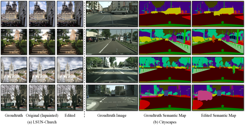
Figure 16: Examples of our synthetic edits on (a) LSUN Church and (b) Cityscapes. On LSUN Church, we view the inpainted image as the original image and generate the edits by quantizing color at the corresponding regions. On Cityscapes, we generate the edits by pasting some foreground objects on the ground-truth semantic maps.

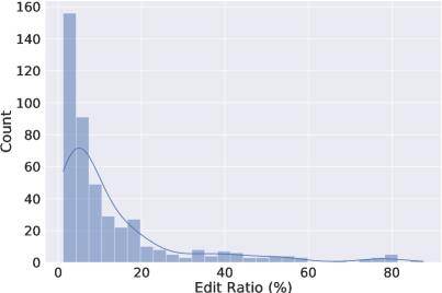
(a)

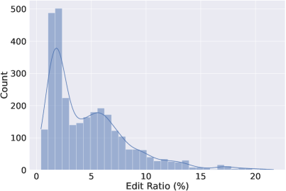
(b)

Figure 17: Detailed edit ratio distribution of our synthetic datasets.

A.2 Shortcut Scatter Fusion

The $1\times 1$ convolution in the shortcut branch consumes much less computation than the convolution in the main branch. Therefore, the overheads of Gather and Scatter weigh more in the shortcut branch. We fuse the Scatter in the shortcut branch and main branch along with residual addition into Scatter with Block Residual to reduce these overheads. Specifically, as shown in Figure 14, we first scatter $F_{l+1}$ output into the pre-computed $F_{l+1}(A^{\text{original}}_{l})+F_{s}(A^{\text{original}}_{l})$ and add the original residual $F_{s}(A^{\text{original}}_{l})$ only at the scattered locations correspondingly according to Indices. Then we calibrate the resulting feature map with $F_{s}$ output by adding the residual difference $F_{s}(A^{\text{edited}}_{l})-F_{s}(A^{\text{original}}_{l})$ at the scattered locations indexed by Shortcut Indices in place.

Appendix B Benchmark Datasets

Below, we elaborate on how we build the synthetic datasets.

LSUN Church. Figure 16(a) shows some examples of our synthetic edits on LSUN Church. The average edited area of the whole dataset is 13.1%. The detailed distribution is shown in Figure LABEL:fig:church-editing.

Cityscapes. We collect 27 foreground object semantic masks from the validation set. The objects include 4 bicycles, 1 motorcycle, 7 cars, 6 trucks, 3 buses, 5 persons, and 1 train. Figure 18(a) visualizes some collected semantic masks. We generate the edits by randomly pasting one of these objects to the ground-truth semantic maps with augmentation. The augmentation includes random horizontal flip, resize (scale factor in $[0.8,1.2]$), and translation ($[-32,32]$ for vertical one and $[-64,64]$ for horizontal one). To make the synthetic edits more reasonable, when the scale factor is larger than 1, the vertical translation can only be positive. Otherwise, it can only be negative. Figure 16(b) shows some edit examples. The average edited area of the entire dataset is 4.77%. The detailed distribution is shown in Figure LABEL:fig:cityscapes-editing.

LAION. We automatically construct our inpainting masks by overlaying circles of random sizes at arbitrary positions. Additional mask examples are displayed in Figure 18(b).

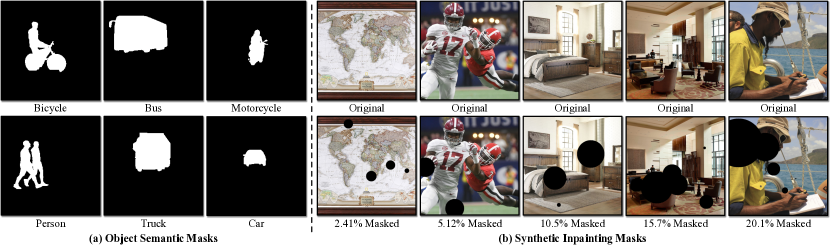
Figure 18: (a) Examples of collected foreground object semantic masks on Cityscapes [13]. (b) Mask examples of the synthetic inpainting datasets on LAION-5B [14].

Method	MACs		PSNR ($\uparrow$)		LPIPS ($\downarrow$)		mIoU ($\uparrow$)
	Value	Ratio	w/ G.T.	w/ Orig.	w/ G.T.	w/ Orig.
Original	281G	–	15.9	–	0.414	–	57.3
GAN Comp. [5]	31.2G	9.0$\times$	15.8	19.1	0.417	0.329	56.3
Ours	30.7G	9.2$\times$	15.9	27.5	0.425	0.076	56.1
0.19 GauGAN	13.3G	21$\times$	15.4	18.4	0.427	0.356	49.5
GAN Comp. (S)	9.64G	29$\times$	15.8	18.9	0.422	0.344	51.2
GAN Comp.+Ours	7.06G	40$\times$	15.8	18.8	0.429	0.345	52.4

TABLE V: Quality evaluation of GauGAN at the edited regions. PSNR/LPIPS w/ G.T. means computing the metrics with the ground-truth images, and w/ Orig. means computing with the generated samples from the original model. 0.19 GauGAN: Reducing each layer of GauGAN to 19% channels and training from scratch. GAN Comp. (S): GAN Compression with larger compression ratio. Our method matches the performance of GAN Compression [5]. When applying it to GAN Compression, our method demonstrates comparable results to GAN Comp. (S) with less computation, achieving a $40\times$ MACs reduction.

Appendix C Additional Results

Quality results at the edited regions. In Table I, we show the quantitative quality results of our method. For DDPM and PD, the unedited areas in the generated images keep the same as the input images due to the mask trick in SDEdit [11]. For GauGAN, the generated unedited regions vary across different methods. In this case, the image quality in these areas will influence the metrics we report in Table I. We also include the quantitative quality results of GauGAN at the edited regions in Table V. Our method could still preserve the image quality of the original GauGAN and match the performance of GAN Compression [5]. When applied to GAN Compression, it reduces $40\times$ MACs on average, achieving results on par with GAN Comp. (S) with less computation.

Additional visualization. In Figure 19, we show more visual results of DDPM [1] and Progressive Distillation [15] on LSUN Church [12]. Besides LSUN Church, we additionally apply SIGE to DDPM on CelebA [109] and AFHQ Dogs [110], as shown in Figure 21, respectively. In Figure 20, we show more visual results of GauGAN on Cityscapes [13]. In Figure 22, we show more visual results of Stable Diffusion [3] on image-to-image translation.

Appendix D License & Computation Resources

Here we show all the licenses of our used assets. Our backbone models DDIM [1], ILVR [33], Progressive Distillation [15], Stable Diffusion, GauGAN [4] and GAN Compression [5] is under MIT license, MIT license, Apache license, CreativeML Open RAIL-M, Creative Commons license and BSD license, respectively. SDEdit is under MIT license. The license of Cityscapes [13] is here. The CelebA [109] license is here. AFHQ-Dogs [110] is under Creative Common license. LSUN Church [12] does not have an explicit license. The examples in Figure 9(a) and Figure 22 are under Creative Commons License. The drawing in Figure 9(b) is created by ourselves, referring to the painting in this link.

Since our method does not involve any model training, all our generated results are obtained on a single NVIDIA RTX 3090, which only takes $1\sim 2$ hours to process all the test images ($\sim 10,000$ in total), including both the original models and our method. We measure the model latency on NVIDIA RTX 3090, 2080Ti, Intel Core i9-10920X CPU, and Apple M1 Pro CPU. On Apple M1 Pro CPU, we use Intel Anaconda for our Python environment.

Appendix E Changelog

V1 Initial preprint release (NeurIPS 2022).

V2 Fix the figure display issue on mobile devices.

V3 (a) Add additional method details. (b) Support attention layers and add the results of Stable Diffusion [3] (Section 7 and Figure 8).

V4 Accepted by T-PAMI. (a) Support MPS backend (Table II). (b) Curate an inpainting benchmark from LAION-5B [14] to evaluate Stable Diffusion [3] (Table I and Figure 8). (c) Expanded large editing analysis (Figure 10). (d) Additional visual results on multiple datasets (Figures 21 and 22).

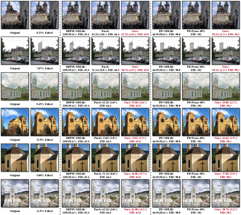
Figure 19: More visual results on LSUN Church of SDEdit with DDPM [1] and Progressive Distillation. MACs measure the computation for a single model forward. Prune 40%: Uniformly pruning 40% weights of the model without fine-tuning. Patch: Cropping the smallest image patch that covers all the edited regions of the model input and blending the model output back to the input image. Our method achieves lower FID with fewer MACs for both DDPM and Progressive Distillation.

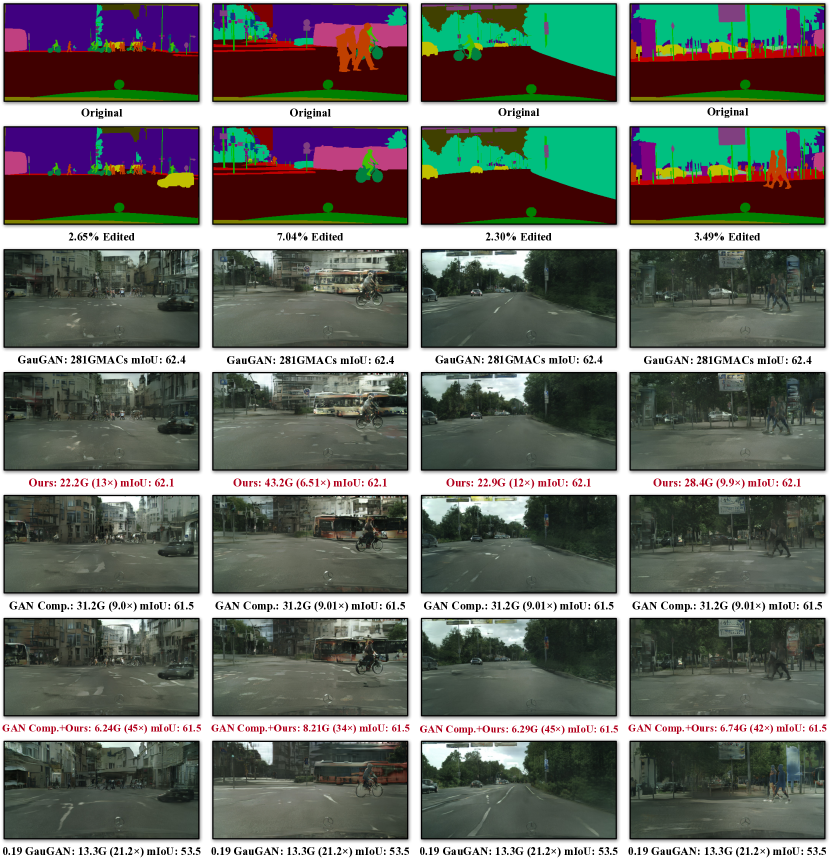
Figure 20: More visual results on Cityscapes of GauGAN [4]. 0.19 GauGAN: Uniformly reducing each layer of GauGAN to 19% channels and training from scratch. Our method could achieve higher mIoU than GAN Compression with fewer MACs. When applying to GAN Compression, our method achieves a $34\sim 45\times$ MACs reduction with a minor mIoU drop.

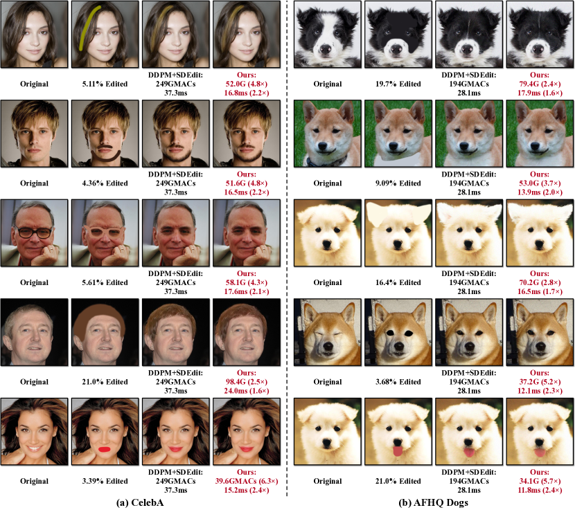
Figure 21: Visual results of DDPM [2] on CelebA [109] and AFHQ Dogs [110]. The computation and latency are measured for a single diffusion step on NVIDIA RTX 3090. SIGE reduces the computation of the original by up to $6.3\times$, achieving an up to $2.4\times$ speedup.

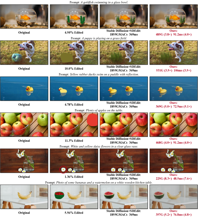
Figure 22: Visual results of Stable Diffusion on text-guided image editing. The computation and latency are measured for a single diffusion step on NVIDIA RTX 3090. SIGE achieves an up to $7.6\times$ speedup under a $1.4\%$ edit.

References

- [1] J. Song, C. Meng, and S. Ermon, “Denoising diffusion implicit models,” in ICLR, 2020.
- [2] J. Ho, A. Jain, and P. Abbeel, “Denoising diffusion probabilistic models,” NeurIPS, 2020.
- [3] R. Rombach, A. Blattmann, D. Lorenz, P. Esser, and B. Ommer, “High-resolution image synthesis with latent diffusion models,” in CVPR, 2022.
- [4] T. Park, M.-Y. Liu, T.-C. Wang, and J.-Y. Zhu, “Semantic image synthesis with spatially-adaptive normalization,” in CVPR, 2019.
- [5] M. Li, J. Lin, Y. Ding, Z. Liu, J.-Y. Zhu, and S. Han, “Gan compression: Efficient architectures for interactive conditional gans,” in CVPR, 2020.
- [6] I. Goodfellow, J. Pouget-Abadie, M. Mirza, B. Xu, D. Warde-Farley, S. Ozair, A. Courville, and Y. Bengio, “Generative adversarial nets,” NeurIPS, 2014.
- [7] T. Karras, S. Laine, and T. Aila, “A style-based generator architecture for generative adversarial networks,” in CVPR, 2019.
- [8] J. Sohl-Dickstein, E. Weiss, N. Maheswaranathan, and S. Ganguli, “Deep unsupervised learning using nonequilibrium thermodynamics,” in ICML, 2015.
- [9] P. Isola, J.-Y. Zhu, T. Zhou, and A. A. Efros, “Image-to-image translation with conditional adversarial networks,” in CVPR, 2017.
- [10] P. Sangkloy, J. Lu, C. Fang, F. Yu, and J. Hays, “Scribbler: Controlling deep image synthesis with sketch and color,” in CVPR, 2017.
- [11] C. Meng, Y. He, Y. Song, J. Song, J. Wu, J.-Y. Zhu, and S. Ermon, “SDEdit: Guided image synthesis and editing with stochastic differential equations,” in ICLR, 2022.
- [12] F. Yu, Y. Zhang, S. Song, A. Seff, and J. Xiao, “Lsun: Construction of a large-scale image dataset using deep learning with humans in the loop,” arXiv preprint arXiv:1506.03365, 2015.
- [13] M. Cordts, M. Omran, S. Ramos, T. Rehfeld, M. Enzweiler, R. Benenson, U. Franke, S. Roth, and B. Schiele, “The cityscapes dataset for semantic urban scene understanding,” in CVPR, 2016.
- [14] C. Schuhmann, R. Beaumont, R. Vencu, C. Gordon, R. Wightman, M. Cherti, T. Coombes, A. Katta, C. Mullis, M. Wortsman et al., “Laion-5b: An open large-scale dataset for training next generation image-text models,” Advances in Neural Information Processing Systems, vol. 35, pp. 25 278–25 294, 2022.
- [15] T. Salimans and J. Ho, “Progressive distillation for fast sampling of diffusion models,” in ICLR, 2021.
- [16] L. Hou, Z. Yuan, L. Huang, H. Shen, X. Cheng, and C. Wang, “Slimmable generative adversarial networks,” in AAAI, 2021.
- [17] Y. Fu, W. Chen, H. Wang, H. Li, Y. Lin, and Z. Wang, “Autogan-distiller: Searching to compress generative adversarial networks,” in ICML, 2020.
- [18] S. Li, M. Lin, Y. Wang, C. Fei, L. Shao, and R. Ji, “Learning efficient gans for image translation via differentiable masks and co-attention distillation,” IEEE Transactions on Multimedia, 2022.
- [19] Q. Jin, J. Ren, O. J. Woodford, J. Wang, G. Yuan, Y. Wang, and S. Tulyakov, “Teachers do more than teach: Compressing image-to-image models,” in CVPR, 2021.
- [20] T. R. Shaham, M. Gharbi, R. Zhang, E. Shechtman, and T. Michaeli, “Spatially-adaptive pixelwise networks for fast image translation,” in CVPR, 2021.
- [21] H. Wang, S. Gui, H. Yang, J. Liu, and Z. Wang, “Gan slimming: All-in-one gan compression by a unified optimization framework,” in ECCV, 2020.
- [22] M. Li, J. Lin, C. Meng, S. Ermon, S. Han, and J.-Y. Zhu, “Efficient spatially sparse inference for conditional gans and diffusion models,” in NeurIPS, 2022.
- [23] M. Ren, A. Pokrovsky, B. Yang, and R. Urtasun, “Sbnet: Sparse blocks network for fast inference,” in CVPR, 2018.
- [24] T. Karras, S. Laine, M. Aittala, J. Hellsten, J. Lehtinen, and T. Aila, “Analyzing and improving the image quality of stylegan,” in CVPR, 2020.
- [25] A. Brock, J. Donahue, and K. Simonyan, “Large scale gan training for high fidelity natural image synthesis,” in ICLR, 2019.
- [26] P. Dhariwal and A. Nichol, “Diffusion models beat gans on image synthesis,” NeurIPS, 2021.
- [27] P. Esser, R. Rombach, and B. Ommer, “Taming transformers for high-resolution image synthesis,” in CVPR, 2021.
- [28] A. Razavi, A. Van den Oord, and O. Vinyals, “Generating diverse high-fidelity images with vq-vae-2,” in NeurIPS, vol. 32, 2019.
- [29] C. Saharia, W. Chan, H. Chang, C. Lee, J. Ho, T. Salimans, D. Fleet, and M. Norouzi, “Palette: Image-to-image diffusion models,” in SIGGRAPH, 2022.
- [30] J.-Y. Zhu, T. Park, P. Isola, and A. A. Efros, “Unpaired image-to-image translation using cycle-consistent adversarial networks,” in ICCV, 2017.
- [31] P. Zhu, R. Abdal, Y. Qin, and P. Wonka, “Sean: Image synthesis with semantic region-adaptive normalization,” in CVPR, 2020.
- [32] A. Nichol, P. Dhariwal, A. Ramesh, P. Shyam, P. Mishkin, B. McGrew, I. Sutskever, and M. Chen, “Glide: Towards photorealistic image generation and editing with text-guided diffusion models,” arXiv preprint arXiv:2112.10741, 2021.
- [33] J. Choi, S. Kim, Y. Jeong, Y. Gwon, and S. Yoon, “Ilvr: Conditioning method for denoising diffusion probabilistic models,” in ICCV, 2021.
- [34] G. Kim and J. C. Ye, “Diffusionclip: Text-guided image manipulation using diffusion models,” arXiv preprint arXiv:2110.02711, 2021.
- [35] J.-Y. Zhu, P. Krähenbühl, E. Shechtman, and A. A. Efros, “Generative visual manipulation on the natural image manifold,” in ECCV, 2016.
- [36] O. Patashnik, Z. Wu, E. Shechtman, D. Cohen-Or, and D. Lischinski, “Styleclip: Text-driven manipulation of stylegan imagery,” in ICCV, 2021.
- [37] R. Abdal, Y. Qin, and P. Wonka, “Image2stylegan: How to embed images into the stylegan latent space?” in ICCV, 2019.
- [38] ——, “Image2stylegan++: How to edit the embedded images?” in CVPR, 2020.
- [39] A. Howard, M. Sandler, G. Chu, L.-C. Chen, B. Chen, M. Tan, W. Wang, Y. Zhu, R. Pang, V. Vasudevan et al., “Searching for mobilenetv3,” in ICCV, 2019.
- [40] A. G. Howard, M. Zhu, B. Chen, D. Kalenichenko, W. Wang, T. Weyand, M. Andreetto, and H. Adam, “Mobilenets: Efficient convolutional neural networks for mobile vision applications,” arXiv preprint arXiv:1704.04861, 2017.
- [41] M. Sandler, A. Howard, M. Zhu, A. Zhmoginov, and L.-C. Chen, “Mobilenetv2: Inverted residuals and linear bottlenecks,” in CVPR, 2018.
- [42] Y. Song, J. Sohl-Dickstein, D. P. Kingma, A. Kumar, S. Ermon, and B. Poole, “Score-based generative modeling through stochastic differential equations,” in ICLR, 2020.
- [43] Z. Kong and W. Ping, “On fast sampling of diffusion probabilistic models,” in ICML Workshop on Invertible Neural Networks, Normalizing Flows, and Explicit Likelihood Models, 2021.
- [44] Z. Xiao, K. Kreis, and A. Vahdat, “Tackling the generative learning trilemma with denoising diffusion GANs,” in ICLR, 2022.
- [45] S. Han, H. Mao, and W. J. Dally, “Deep Compression: Compressing Deep Neural Networks with Pruning, Trained Quantization and Huffman Coding,” in ICLR, 2016.
- [46] Y. He, J. Lin, Z. Liu, H. Wang, L.-J. Li, and S. Han, “AMC: AutoML for Model Compression and Acceleration on Mobile Devices,” in ECCV, 2018.
- [47] J. Lin, Y. Rao, J. Lu, and J. Zhou, “Runtime neural pruning,” in NeurIPS, 2017.
- [48] Y. He, X. Zhang, and J. Sun, “Channel pruning for accelerating very deep neural networks,” in ICCV, 2017.
- [49] Z. Liu, J. Li, Z. Shen, G. Huang, S. Yan, and C. Zhang, “Learning efficient convolutional networks through network slimming,” in ICCV, 2017.
- [50] Z. Liu, H. Mu, X. Zhang, Z. Guo, X. Yang, K.-T. Cheng, and J. Sun, “MetaPruning: Meta Learning for Automatic Neural Network Channel Pruning,” in ICCV, 2019.
- [51] S. Zhou, Y. Wu, Z. Ni, X. Zhou, H. Wen, and Y. Zou, “Dorefa-net: Training low bitwidth convolutional neural networks with low bitwidth gradients,” arXiv preprint arXiv:1606.06160, 2016.
- [52] M. Rastegari, V. Ordonez, J. Redmon, and A. Farhadi, “Xnor-net: Imagenet classification using binary convolutional neural networks,” in ECCV, 2016.
- [53] K. Wang, Z. Liu, Y. Lin, J. Lin, and S. Han, “Haq: Hardware-aware automated quantization with mixed precision,” in CVPR, 2019.
- [54] J. Choi, Z. Wang, S. Venkataramani, P. I.-J. Chuang, V. Srinivasan, and K. Gopalakrishnan, “Pact: Parameterized clipping activation for quantized neural networks,” arXiv preprint arXiv:1805.06085, 2018.
- [55] B. Jacob, S. Kligys, B. Chen, M. Zhu, M. Tang, A. Howard, H. Adam, and D. Kalenichenko, “Quantization and training of neural networks for efficient integer-arithmetic-only inference,” in CVPR, 2018.
- [56] B. Zoph and Q. V. Le, “Neural Architecture Search with Reinforcement Learning,” in ICLR, 2017.
- [57] B. Zoph, V. Vasudevan, J. Shlens, and Q. V. Le, “Learning Transferable Architectures for Scalable Image Recognition,” in CVPR, 2018.
- [58] H. Liu, K. Simonyan, and Y. Yang, “DARTS: Differentiable Architecture Search,” in ICLR, 2019.
- [59] H. Cai, L. Zhu, and S. Han, “ProxylessNAS: Direct Neural Architecture Search on Target Task and Hardware,” in ICLR, 2019.
- [60] M. Tan, B. Chen, R. Pang, V. Vasudevan, M. Sandler, A. Howard, and Q. V. Le, “MnasNet: Platform-Aware Neural Architecture Search for Mobile,” in CVPR, 2019.
- [61] B. Wu, X. Dai, P. Zhang, Y. Wang, F. Sun, Y. Wu, Y. Tian, P. Vajda, Y. Jia, and K. Keutzer, “FBNet: Hardware-Aware Efficient ConvNet Design via Differentiable Neural Architecture Search,” in CVPR, 2019.
- [62] J. Lin, W.-M. Chen, Y. Lin, J. Cohn, C. Gan, and S. Han, “Mcunet: Tiny deep learning on iot devices,” in NeurIPS, 2020.
- [63] J. Lin, R. Zhang, F. Ganz, S. Han, and J.-Y. Zhu, “Anycost gans for interactive image synthesis and editing,” in CVPR, 2021.
- [64] H. Shu, Y. Wang, X. Jia, K. Han, H. Chen, C. Xu, Q. Tian, and C. Xu, “Co-evolutionary compression for unpaired image translation,” in ICCV, 2019.
- [65] Y. Liu, Z. Shu, Y. Li, Z. Lin, F. Perazzi, and S.-Y. Kung, “Content-aware gan compression,” in CVPR, 2021.
- [66] R. Ma and J. Lou, “Cpgan: An efficient architecture designing for text-to-image generative adversarial networks based on canonical polyadic decomposition,” Scientific Programming, 2021.
- [67] A. Aguinaldo, P.-Y. Chiang, A. Gain, A. Patil, K. Pearson, and S. Feizi, “Compressing gans using knowledge distillation,” arXiv preprint arXiv:1902.00159, 2019.
- [68] S. Han, J. Pool, J. Tran, and W. Dally, “Learning both weights and connections for efficient neural network,” NeurIPS, 2015.
- [69] H. Li, A. Kadav, I. Durdanovic, H. Samet, and H. P. Graf, “Pruning filters for efficient convnets,” ICLR, 2016.
- [70] B. Liu, M. Wang, H. Foroosh, M. Tappen, and M. Pensky, “Sparse convolutional neural networks,” in CVPR, 2015.
- [71] M. Jaderberg, A. Vedaldi, and A. Zisserman, “Speeding up convolutional neural networks with low rank expansions,” in BMVC, 2014.
- [72] H. Tang, Z. Liu, X. Li, Y. Lin, and S. Han, “Torchsparse: Efficient point cloud inference engine,” in MLSys, 2022.
- [73] G. Riegler, A. Osman Ulusoy, and A. Geiger, “Octnet: Learning deep 3d representations at high resolutions,” in CVPR, 2017.
- [74] P. Judd, A. Delmas, S. Sharify, and A. Moshovos, “Cnvlutin2: Ineffectual-activation-and-weight-free deep neural network computing,” arXiv preprint arXiv:1705.00125, 2017.
- [75] S. Shi and X. Chu, “Speeding up convolutional neural networks by exploiting the sparsity of rectifier units,” arXiv preprint arXiv:1704.07724, 2017.
- [76] X. Dong, J. Huang, Y. Yang, and S. Yan, “More is less: A more complicated network with less inference complexity,” in CVPR, 2017.
- [77] B. Pan, W. Lin, X. Fang, C. Huang, B. Zhou, and C. Lu, “Recurrent residual module for fast inference in videos,” in CVPR, 2018.
- [78] X. Li, Z. Liu, P. Luo, C. Change Loy, and X. Tang, “Not all pixels are equal: Difficulty-aware semantic segmentation via deep layer cascade,” in CVPR, 2017.
- [79] T. Verelst and T. Tuytelaars, “Dynamic convolutions: Exploiting spatial sparsity for faster inference,” in CVPR, 2020.
- [80] L. Wang, X. Dong, Y. Wang, X. Ying, Z. Lin, W. An, and Y. Guo, “Exploring sparsity in image super-resolution for efficient inference,” in CVPR, 2021.
- [81] Y. Han, G. Huang, S. Song, L. Yang, Y. Zhang, and H. Jiang, “Spatially adaptive feature refinement for efficient inference,” TIP, 2021.
- [82] Y. Wang, Y. Yue, Y. Lin, H. Jiang, Z. Lai, V. Kulikov, N. Orlov, H. Shi, and G. Huang, “Adafocus v2: End-to-end training of spatial dynamic networks for video recognition,” in CVPR, 2022.
- [83] M. Parger, C. Tang, C. D. Twigg, C. Keskin, R. Wang, and M. Steinberger, “Deltacnn: End-to-end cnn inference of sparse frame differences in videos,” in CVPR, 2022.
- [84] S. Ioffe and C. Szegedy, “Batch normalization: Accelerating deep network training by reducing internal covariate shift,” in ICML, 2015.
- [85] D. Ulyanov, A. Vedaldi, and V. Lempitsky, “Instance normalization: The missing ingredient for fast stylization,” arXiv preprint arXiv:1607.08022, 2016.
- [86] X. Huang and S. Belongie, “Arbitrary style transfer in real-time with adaptive instance normalization,” in ICCV, 2017.
- [87] Y. Wu and K. He, “Group normalization,” in ECCV, 2018.
- [88] A. Q. Nichol and P. Dhariwal, “Improved denoising diffusion probabilistic models,” in ICML, 2021.
- [89] Y. Ding, L. Zhu, Z. Jia, G. Pekhimenko, and S. Han, “Ios: Inter-operator scheduler for cnn acceleration,” MLSys, 2021.
- [90] Z. Jia, O. Padon, J. Thomas, T. Warszawski, M. Zaharia, and A. Aiken, “Taso: optimizing deep learning computation with automatic generation of graph substitutions,” in SOSP, 2019.
- [91] K. He, X. Zhang, S. Ren, and J. Sun, “Deep residual learning for image recognition,” in CVPR, 2016.
- [92] H. Zhang, I. Goodfellow, D. Metaxas, and A. Odena, “Self-attention generative adversarial networks,” in ICML, 2019.
- [93] A. Vaswani, N. Shazeer, N. Parmar, J. Uszkoreit, L. Jones, A. N. Gomez, Ł. Kaiser, and I. Polosukhin, “Attention is all you need,” NeurIPS, 2017.
- [94] O. Ronneberger, P. Fischer, and T. Brox, “U-net: Convolutional networks for biomedical image segmentation,” in Medical Image Computing and Computer-Assisted Intervention–MICCAI 2015: 18th International Conference, Munich, Germany, October 5-9, 2015, Proceedings, Part III 18. Springer, 2015, pp. 234–241.
- [95] G. Hinton, O. Vinyals, J. Dean et al., “Distilling the knowledge in a neural network,” arXiv preprint arXiv:1503.02531, vol. 2, no. 7, 2015.
- [96] X. Zhou, R. Girdhar, A. Joulin, P. Krähenbühl, and I. Misra, “Detecting twenty-thousand classes using image-level supervision,” in arXiv preprint arXiv:2201.02605, 2021.
- [97] S. Zhao, J. Cui, Y. Sheng, Y. Dong, X. Liang, E. I. Chang, and Y. Xu, “Large scale image completion via co-modulated generative adversarial networks,” in ICLR, 2021.
- [98] R. Zhang, P. Isola, A. A. Efros, E. Shechtman, and O. Wang, “The unreasonable effectiveness of deep features as a perceptual metric,” in CVPR, 2018.
- [99] M. Heusel, H. Ramsauer, T. Unterthiner, B. Nessler, and S. Hochreiter, “Gans trained by a two time-scale update rule converge to a local nash equilibrium,” NeurIPS, 2017.
- [100] G. Parmar, R. Zhang, and J.-Y. Zhu, “On aliased resizing and surprising subtleties in gan evaluation,” in CVPR, 2022.
- [101] F. Yu, V. Koltun, and T. Funkhouser, “Dilated residual networks,” in CVPR, 2017.
- [102] C. Lu, Y. Zhou, F. Bao, J. Chen, C. Li, and J. Zhu, “Dpm-solver: A fast ode solver for diffusion probabilistic model sampling in around 10 steps,” arXiv preprint arXiv:2206.00927, 2022.
- [103] ——, “Dpm-solver++: Fast solver for guided sampling of diffusion probabilistic models,” arXiv preprint arXiv:2211.01095, 2022.
- [104] D. Watson, J. Ho, M. Norouzi, and W. Chan, “Learning to efficiently sample from diffusion probabilistic models,” arXiv preprint arXiv:2106.03802, 2021.
- [105] C. Meng, R. Gao, D. P. Kingma, S. Ermon, J. Ho, and T. Salimans, “On distillation of guided diffusion models,” arXiv preprint arXiv:2210.03142, 2022.
- [106] Y. Shang, Z. Yuan, B. Xie, B. Wu, and Y. Yan, “Post-training quantization on diffusion models,” arXiv preprint arXiv:2211.15736, 2022.
- [107] X. Li, L. Lian, Y. Liu, H. Yang, Z. Dong, D. Kang, S. Zhang, and K. Keutzer, “Q-diffusion: Quantizing diffusion models,” arXiv preprint arXiv:2302.04304, 2023.
- [108] S.-Y. Wang, O. Wang, R. Zhang, A. Owens, and A. A. Efros, “Cnn-generated images are surprisingly easy to spot… for now,” in CVPR, 2020.
- [109] Z. Liu, P. Luo, X. Wang, and X. Tang, “Deep learning face attributes in the wild,” in ICCV, 2015.
- [110] Y. Choi, Y. Uh, J. Yoo, and J.-W. Ha, “Stargan v2: Diverse image synthesis for multiple domains,” in CVPR, 2020.