To spike or not to spike: the whims of the Wonham filter in the strong noise regime

Abstract.

We study the celebrated Shiryaev-Wonham filter in its historical setup [Won64] where the hidden Markov jump process has two states. We are interested in the weak noise regime for the observation equation. Interestingly, this becomes a strong noise regime for the filtering equations.

Earlier results of the authors show the appearance of spikes in the filtered process, akin to a metastability phenomenon. This paper is aimed at understanding the smoothed optimal filter, which is relevant for any system with feedback. In particular, we demonstrate that there is a sharp phase transition between a spiking regime and a regime with perfect smoothing.

 

 

1. Introduction

Filtering Theory adresses the problem of estimating a hidden process ${\mathbf{x}}=({\mathbf{x}}_{t}\;;\;t\geq 0)$ which can not be directly observed. At hand, one has access to an observation process which is naturally correlated to ${\mathbf{x}}$. The most simple setup, called the “signal plus noise” model, is the one where the observation process ${\mathbf{y}}^{\gamma}=({\mathbf{y}}^{\gamma}_{t}\;;\;t\geq 0)$ is of the form

$$d{\mathbf{y}}^{\gamma}_{t}={\mathbf{x}}_{t}dt+\cfrac{1}{\sqrt{\gamma}}\ dB_{t}$$ (1.1)

where $B=(B_{t}\;;\;t\geq 0)$ is a standard Wiener process and $\gamma>0$. Moreover it is natural to assume that the noise is intrinsic to the observation system, so that the Brownian motion $B=B^{\gamma}$ has no reason of being the same for different values of $\gamma$. See Figure 1.1 for an illustration which visually highlights the difficulty of recognizing a drift despite Brownian motion fluctuations. In this paper we shall focus on the case where $(\textbf{x}_{t}\;;\;t\geq 0)$ is a pure jump Markov process on $\{0,1\}$ with càdlàg trajectories. We denote $\lambda p$ (resp. $\lambda(1-p)$) the jump rate between $0$ and $1$ (resp. between $1$ and $0$), with $p\in(0,1)$ and $\lambda>0$. This is the historical setting of the celebrated Wonham filter [Won64, Eq. (19)].

In the mean square sense, the best estimator taking value in $\{0,1\}$ at time $t$ of $\textbf{x}_{t}$, given the observation $({\textbf{y}}^{\gamma}_{s})_{s\leq t}$, is equal to

$${\hat{\mathbf{x}}^{\gamma}}_{t}= \ \mathds{1}_{\left\{\pi^{\gamma}_{t}>\frac{1}{2}\right\}}$$ (1.2)

where $\pi^{\gamma}_{t}$ is the conditional probability

$$\pi^{\gamma}_{t}:= \ {\mathbb{P}}\left({\bf x}_{t}=1\ |\ \left({\bf y}^{\gamma}_{s}\right)_{s\leq t}\right)\ .$$ (1.3)

Our interest lies in the situation where the intensity $1/\sqrt{\gamma}$ of the observation noise is small, i.e. $\gamma$ is large. At first glance, one could argue that weak noise limits for the observation process are not that interesting because we are dealing with extremely reliable systems since they are subject to very little noise. This paper aims at demonstrating that this regime is interesting from both a theoretical and a practical point of view.

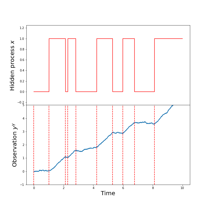
Figure 1.1. Numerical simulation of the hidden process ${\mathbf{x}}$ and the observation process ${\mathbf{y}}^{\gamma}$ for $\gamma=10^{2}$. The challenge is to infer the drift of ${\mathbf{y}}^{\gamma}$, in spite of Brownian noise and in a very short window. Parameters are $\lambda=1.3$ and $p=0.4$. There are $10^{6}$ time steps to discretize $[0,10]$. The code is available at the online repository                             %\quad␣\quad␣\quad␣\quadhttps://github.com/redachhaibi/Spikes-in-Classical-Filtering

A motivating example. Let us describe a simple situation that falls into that scope and motivates our study. Consider for example a single classical bit – say, inside of a DRAM chip. The value of the bit is subject to changes, some of which are caused by CPU instructions and computations, some of which are due to errors. The literature points to spontaneous errors due to radiation, heat and various conditions [SPW09]. The value of that process is modeled by the Markov process ${\mathbf{x}}$ as defined above. Here, the process ${\bf y}^{\gamma}$ is the electric current received by a sensor on the chip, which monitors any changes. Any retroaction, for example code correction in ECC memory [KLK⁺14, PKHM19], requires the observation during a finite window $\delta>0$. And the reaction is at best instantaneous. For anything meaningful to happen, everything depends thus on the behavior of:

$$\pi_{t}^{\delta,\gamma}:= \ {\mathbb{P}}\left({\bf x}_{t-\delta}=1\ |\ \left({\bf y}^{\gamma}_{s}\right)_{s\leq t}\right)\ ,$$ (1.4)

and instead to consider the estimator ${\hat{x}}_{t}^{\gamma}$ given by Eq. (1.2), we are left with the estimator

$${\hat{\mathbf{x}}^{\delta,\gamma}}_{t}=\mathds{1}_{\left\{\pi^{\delta,\gamma}_{t}>\frac{1}{2}\right\}}\ .$$

From an engineering point of view, it is the interplay between different time scales which is important in order to design a system with high performance: if the noise is weak, how fast can a feed-back response be? For a given process $z=({z}_{t}\;;t\geq 0)$ with values in $[0,1]$ we denote the hitting time of $(\frac{1}{2},1)$ by $T({z}):=\inf\left\{t\geq 0\;;\;{z}_{t}>\frac{1}{2}\right\}$. Assume for example that initially ${\bf x}_{0}=0$. For a given time $t>0$, a natural problem is to estimate, as $\gamma\to\infty$, the probability to predict a false value of the bit given its value remains equal to $0$ during the time interval $[0,t]$, i.e.

$${\mathbb{P}}\left(T({\hat{\mathbf{x}}}^{\delta,\gamma})\leq t\;|\;T({\bf x})>t\right)\ .$$ (1.5)

1.1. Informal statement of the result.

A consequence of the results of this paper is the precise identification of the regimes $\delta:=\delta(\gamma)$ for which the probability in (1.5) vanishes or not as $\gamma\to\infty$:

• If $\limsup_{\gamma\to\infty}\delta(\gamma)\tfrac{\gamma}{\log\gamma}<2$, i.e. $\delta$ is too small, the retroaction/control system can be surprised by a spike, causing a misfire in detecting the regime change and the limiting error probability in Eq. (1.5) is equal to $1-\exp\left(-\lambda pt\right)$;
  

• If $\liminf_{\gamma\to\infty}\delta(\gamma)\tfrac{\gamma}{\log\gamma}>2$, i.e. $\delta$ is sufficiently large, the estimator will be very good at detecting jumps of the Markov process ${\bf x}$, the limiting error probability in Eq. (1.5) vanishing, however the reaction time will deteriorate.
  

While the literature usually focuses on $L^{2}(\Omega)$ considerations for filtering processes, we focus on this article on pathwise properties of the filtering process under investigation when $\gamma\rightarrow\infty$. Indeed, it is clear that the question addressed just above cannot be answered in an $L^{2}(\Omega)$ framework only.

Let us now present in some informal way the reasons for which we have this difference of behavior. As it will be recalled later the process $\pi^{\gamma}=\left(\pi^{\gamma}_{t}\ ;\ t\geq 0\right)$ satisfies in law

$$d\pi^{\gamma}_{t}=-\lambda\left(\pi^{\gamma}_{t}-p\right)dt+\sqrt{\gamma}\pi^{\gamma}_{t}\left(1-\pi^{\gamma}_{t}\right)dW_{t}\ ,$$ (1.6)

where $W=(W_{t}\;;\;t\geq 0)$ is a Brownian motion with a now strong parameter $\sqrt{\gamma}$ in front of it. This is the so called Shiryaev-Wonham filtering theory. As shown in [BCC⁺22], when $\gamma$ goes to infinity the process $\pi^{\gamma}$ converges in law to an unusual and singular process in a suitable topology (see Figure 1.2). Indeed as exhibited in the figure, the limiting process is the Markov jump process $({\bf x}_{t}\;;\;t\geq 0)$ but decorated with vertical lines, called spikes, whose extremities are distributed according an inhomogeneous point Poisson process. As we can observe on Figure 1.3 if $\delta$ is sufficiently large, the spikes in the process $\pi^{\gamma,\delta}$ are suppressed while if $\delta$ is sufficiently small they survive. The spikes are responsible of the non vanishing error probability in Eq. (1.5) since they are interpreted by the estimator ${\hat{\mathbf{x}}}^{\delta,\gamma}$ as a jump from $0$ to $1$ of the process $\bf x$. The fact that the transition between the two regimes is precisely $2\frac{\log\gamma}{\gamma}$ is more complicated to explain without going into computational details. Building on our earlier results, we examine hence in this paper the effect of smoothing and the relevance of various time scales required for filtering, smoothing and control in the design of a system with feedback.

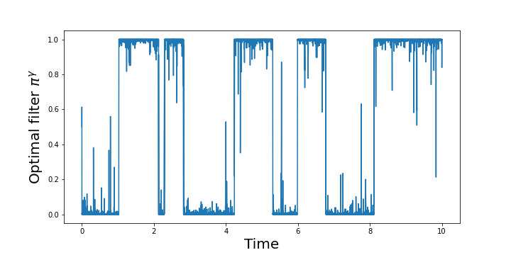
Figure 1.2. “The whims of the Wonham filter”: Informally, on a very short time interval, it is difficult to distinguish between a change in the drift of ${\mathbf{y}}^{\gamma}$ and an exceptionnal time of Brownian motion. The figure shows a numerical simulation of the process $\left(\pi_{t}^{\gamma}\ ;\ t\geq 0\right)$ for the same realization of ${\mathbf{x}}$ as Fig. 1.1. Same time discretization. This time we chose the larger $\gamma=10^{4}$ to highlight spikes.

Figure 1.3. Numerical simulation of the process $\left(\pi_{t}^{\delta,\gamma}\ ;\ t\geq 0\right)$ for the same realization of ${\mathbf{x}}$ as Fig. 1.1. Same time discretisation. We have $\gamma=10^{4}$ and $\delta_{\gamma}=C\frac{\log\gamma}{\gamma}$, with $C\in\{\frac{1}{2},1,2,4,8\}$.

Remark 1.1 (Duality between weak and strong noise).

Notice that the observation equation (1.1) has a factor $\frac{1}{\sqrt{\gamma}}$, while the filtering equation (1.6) has a factor $\sqrt{\gamma}$. This is a well-known duality between the weak noise limit in the observation process and the strong noise limit filtered state.

In fact, when analyzing the derivation of the Wonham-Shiryaev filter, this is simply due to writing:

$$d{\bf y}^{\gamma}_{t}=\frac{1}{\sqrt{\gamma}}\left(dB_{t}+\sqrt{\gamma}{\mathbf{x}}_{t}dt\right)=:\frac{1}{\sqrt{\gamma}}dW^{\mathbb{Q}}_{t}\ ,$$

and using the Girsanov transform to construct a new measure ${\mathbb{Q}}$, for the Kallianpur-Streibel formula, under which $W^{\mathbb{Q}}$ is a Brownian motion – [VH07, Chapter 7].

1.2. Literature review of filtering theory in the $\gamma\rightarrow\infty$ regime.

The understanding of the behavior of the classical filter for jump Markov processes with small Brownian observation noise has attracted some attention in the 90’s. Most of the work focused on the long time regime [Won64, KL92, KZ96, AZ97b, AZ97a, Ass97], by studying for example stationary measures, asymptotic stability or transmission rates. In the case where the jump Markov process is replaced by a diffusion process with a signal noise, possibly small, [Pic86, AZ98] study the efficiency (in the $L^{2}$ sense and at fixed time) of some asymptotically optimal filters. In [PZ05] are obtained quenched large deviations principles for the distribution of the optimal filter at a fixed time for one dimensional nonlinear filtering in the small observation noise regime – see also [RBA22]. In a similar context Atar obtains in [Ata98] some non-optimal upper bounds for the asymptotic rate of stability of the filter.

Going through the aforementioned literature one can observe that the term $\log(\gamma)/\gamma$ already appears in those references. Indeed the quantities of interest include the (average) long time error rate [Ass97, Eq. (1.4)]

$$\alpha^{*}=\lim_{t\to\infty}\frac{1}{t}\int_{0}^{t}\min(\pi_{s}^{\gamma},1-\pi_{s}^{\gamma})ds$$

or the probability of error in long time ([Won64] and [KZ96, Theorem 1’])

$$\mathcal{P}_{err}(\gamma)=\lim_{t\to\infty}\inf_{\zeta\in L_{\infty}(\mathcal{F}_{t}^{{\mathbf{y}}})}\mathbb{P}(\zeta\neq{\mathbf{x}}_{t})=\lim_{t\to\infty}{\mathbb{P}}(\hat{\mathbf{x}}_{t}\neq{\mathbf{x}}_{t})$$

or the long time mean squared error [Gol00]

$${\mathcal{E}}_{mse}(\gamma)=\lim_{t\to\infty}\inf_{\zeta\in L_{\infty}(\mathcal{F}_{t}^{{\mathbf{y}}})}\mathbb{E}(\zeta-{\mathbf{x}}_{t})^{2}=\lim_{t\to\infty}\mathbb{E}(\pi_{t}^{\gamma}-{\mathbf{x}}_{t})^{2}\ .$$

Here ${\mathcal{F}}^{{\mathbf{y}}}$ denotes the natural filtration of ${\mathbf{y}}={\mathbf{y}}^{\gamma}$. These quantities are shown to be of order $\log(\gamma)/\gamma$ up to a constant which is related to the invariant measure of ${\mathbf{x}}$ and some relative entropy but which is definitively not $2$ – see [Gol00, Eq. (3)]. Note that all these quantities are of asymptotic nature and their analysis goes through the invariant measure. Beyond the appearance of the quantity $\log(\gamma)/\gamma$, which is fortuitous, our results are of a completely different nature since we want to obtain a sharp result on a fixed finite time interval. Also, due to the spiking phenomenon and the singularity of the involved processes, there is no chance that the limits can be exchanged.

To the best of the authors’ knowledge, this paper is the first of its kind to aim for a trajectorial description of the limit, in the context of classical filtering theory. However, the spiking phenomenon has first been identified in the context of quantum filtering [Mab09, Fig. 2] and more specifically, for the control and error correction of qubits. The spiking phenomenon is already seen as a possible source of error where correction can be made while no error has occurred. To quote [Mab09, Section 4], when discussing the relevance of the optimal Wonham filter in the strong noise regime, it “is not a good measure of the information content of the system, as it is very sensitive to the whims of the filter”.

Then, in the studies of quantum trajectories with strong measurement, a flurry of developments have recently taken place, following the pioneering works of Bauer, Bernard and Tilloy [TBB15, BBT16]. Strong interaction with the environment, which is natural in the quantum setting, corresponds to a strong noise in the quantum trajectories.

Note that, the SDEs are the same when comparing classical to quantum filtering. Nevertheless, the noise has a fundamentally different nature. And there is no hidden process ${\mathbf{x}}$ in the quantum setting. See [BBC⁺21, BCC⁺22] for a recent account and more references on the quantum literature.

2. Statement of the problem and Main Theorem

2.1. The Shiryaev-Wonham filter

Let us start by presenting the Shiryaev-Wonham filter and refer to [Won64, Lip01, VH07] for more extensive material.

2.1.1. General setup

In this paragraph only, we present the Shiryaev-Wonham filter on $n$ states, which will allow to highlight the structural aspects of Eq. (1.6) and later make comments on the general setting. In general, one considers a Markov process ${\mathbf{x}}=\left({\mathbf{x}}_{t}\ ;\ t\geq 0\right)$ on a finite state space $E=\{x_{1},x_{2},\dots,x_{n}\}$ and a continuous observation process ${\bf y}^{\gamma}$ of the usual additive form “signal plus noise”:

$$d{\bf y}^{\gamma}_{t}:= \ G\left({\mathbf{x}}_{t}\right)dt+\frac{1}{\sqrt{\gamma}}dB_{t}\ .$$

Here $G:E\rightarrow{\mathbb{R}}$ is a function taking distinct values for identifiability purposes. The filtered state is given by:

$$\rho^{\gamma}_{t}(x_{i}):={\mathbb{P}}\left({\mathbf{x}}_{t}=x_{i}\ |\ \left({\bf y}^{\gamma}_{s}\right)_{s\leq t}\right)\ .$$

The generator of ${\mathbf{x}}$ is denoted by ${\mathcal{L}}$. The claim of the Shiryaev-Wonham filter is that the filtering equation becomes:

$$\begin{split}d\rho^{\gamma}_{t}(x_{i})=&\ \sum_{j}\left(\rho^{\gamma}_{t}(x_{j}){\mathcal{L}}(x_{j},x_{i})-\rho^{\gamma}_{t}(x_{i}){\mathcal{L}}(x_{i},x_{j})\right)dt+\sqrt{\gamma}\rho^{\gamma}_{t}(x_{i})\left(G(x_{i})-\langle\rho^{\gamma}_{t},G\rangle\right)dW_{t}\ .\end{split}$$ (2.1)

Here $W$ is the innovation process, and is a ${\mathcal{F}}^{{\mathbf{y}}}$-standard Brownian motion. The quantity $\langle\rho^{\gamma}_{t},G\rangle$ denotes the expectation of $G$ with respect to the probability measure $\rho_{t}^{\gamma}$. Throughout the paper, we only consider $E=\{0,1\}$, i.e. the two state regime.

2.1.2. Two states

In this case, all the information is contained in

$$\pi_{t}^{\gamma}:=\rho^{\gamma}_{t}(1)={\mathbb{P}}\left({\mathbf{x}}_{t}=1\ |\ \left({\bf y}^{\gamma}_{s}\right)_{s\leq t}\right)\ .$$

Making explicit in this case Eq. (2.1) we observe that is has exactly the same type of dynamic as the one studied in the authors’ previous paper [BCC⁺22]. Using the notation

$${\mathcal{L}}=\begin{pmatrix}-\lambda_{0,1}&\lambda_{0,1}\\ \lambda_{1,0}&-\lambda_{1,0}\\ \end{pmatrix}\ .$$

we have indeed that Eq. (2.1) can be rewritten as

$$d\pi^{\gamma}_{t}=-\lambda\left(\pi^{\gamma}_{t}-p\right)dt+\sqrt{\gamma}\sigma\pi^{\gamma}_{t}\left(1-\pi^{\gamma}_{t}\right)dW_{t}\ ,$$

where

$$\lambda=\lambda_{0,1}+\lambda_{1,0}\ ,\quad p=\lambda_{1,0}/\lambda\ ,\quad\sigma=G^{1}-G^{0}\ .$$ (2.2)

Without loss of generality, we shall assume $\sigma=1$ in the rest of the paper. Also $(G^{0},G^{1})=(0,1)$. In the end, our setup is indeed given by Eq. (1.1) and (1.6), which we repeat for convenience:

$$d{\bf y}^{\gamma}_{t}= \ {\mathbf{x}}_{t}dt+\frac{1}{\sqrt{\gamma}}dB_{t}\ ,$$ (2.3)

$$d\pi^{\gamma}_{t}= -\lambda\left(\pi^{\gamma}_{t}-p\right)dt+\sqrt{\gamma}\pi^{\gamma}_{t}\left(1-\pi^{\gamma}_{t}\right)dW_{t}\ .$$ (2.4)

Remark 2.1.

The invariant probability measure $\mu$ of the Markov process ${\mathbf{x}}$ solves

$${\mathcal{L}}^{*}\mu=0\Longleftrightarrow\mu=\begin{bmatrix}p\\ 1-p\end{bmatrix}\ .$$

Without any computation, this is intuitively clear, as setting $\gamma\rightarrow 0$ yields an extremely strong observation noise and no noise in the filtering equation:

$$d\pi^{\gamma=0}_{t}=-\lambda(\pi_{t}^{\gamma=0}-p)dt$$

whose asymptotic value is $p$. Informally, this says that, in the absence of information, the best estimation of the law ${\mathcal{L}}({\mathbf{x}}_{t})$ in long time is the invariant measure. This is essentially the content of [Chi06, Theorem 4], which holds for a Shiryaev-Wonham filter with any finite number of states.

2.1.3. Innovation process

The innovation appearing in the SDE is the ${\mathcal{F}}^{{\mathbf{y}}}$-Brownian motion obtained as:

$$dW_{t}=\sqrt{\gamma}\left(d{\mathbf{y}}_{t}-\langle G,\rho_{t}\rangle dt\right)=dB_{t}+\sqrt{\gamma}\left(G({\mathbf{x}}_{t})-\langle G,\rho_{t}\rangle\right)dt\ .$$

With the simplifying assumption that $(G^{0},G^{1})=(0,1)$, we obtain:

$$dW_{t}=dB_{t}+\sqrt{\gamma}\left({\mathbf{x}}_{t}-\pi_{t}^{\gamma}\right)dt\ .$$ (2.5)

2.2. Trajectorial strong noise limits and the question

Eq. (1.6) falls in the scope of [BCC⁺22] which treats the strong noise limits of a large class of one-dimensional SDEs. There the authors give a general result for SDEs not necessarily related to filtering theory. More precisely, the result is two-fold. On the one hand, the process $\pi^{\gamma}$ converges in a weak “Lebesgue-type” topology to a Markov jump process. On the other hand, if one considers a strong “uniform-type” it is possible to capture the convergence to a spike process.

Fixing an arbitrary horizon time $H>0$ . The weaker topology uses the distance:

$${\rm d}_{\mathbb{L}}(f,g):=\int_{0}^{H}\left(\left|f(t)-g(t)\right|\wedge 1\right)dt\ ,$$ (2.6)

inducing the Lebesgue $\mathbb{L}^{0}$ topology on the compact set $[0,H]$. Notice that the previous paper [BCC⁺22] deals with an infinite time horizon. Of course, the restricted topology is the same.

The stronger topology is defined by using the Hausdorff distance for graphs. In this paper, a graph is nothing but a closed (hence compact) subset ${\mathcal{G}}=\bigsqcup_{t\in[0,H]}(\{t\}\times{\mathcal{G}}_{t})$ of $[0,H]\times\mathbb{[}0,1]$, where ${\mathcal{G}}_{t}=\{x\in[0,1]\;;\;(t,x)\in{\mathcal{G}}\}$ denotes the slice of the graph ${\mathcal{G}}$ at time $t$. The Hausdorff distance ${\rm d}_{\mathbb{H}}({\mathcal{G}},{\mathcal{G}}^{\prime})$ between two graphs ${\mathcal{G}}$ and ${\mathcal{G}}^{\prime}$ is then defined by:

$${\rm d}_{{\mathbb{H}}}({\mathcal{G}},{\mathcal{G}}^{\prime}):= \ \inf\left\{\varepsilon>0\ |\ {\mathcal{G}}\subset{\mathcal{G}}^{\prime}+\varepsilon{\mathbb{B}}\ ,\ {\mathcal{G}}^{\prime}\subset{\mathcal{G}}+\varepsilon{\mathbb{B}}\right\}=\max_{\begin{subarray}{c}z\in{\mathcal{G}}\\ z^{\prime}\in{\mathcal{G}}^{\prime}\end{subarray}}\left\{{\rm d}(z,{\mathcal{G}}^{\prime}),{\rm d}(z^{\prime},{\mathcal{G}})\right\}$$ (2.7)

where ${\mathbb{B}}$ is the unit ball of ${\mathbb{R}}^{2}$ and, for $a\in\mathbb{R}^{2}$ and $B\subset\mathbb{R}^{2}$, ${\rm d}(a,B)=\inf_{b\in B}\|a-b\|$. This distance is the appropriate one which allow to capture the spiking process. Indeed, when interpreting in terms of processes, this distance corresponds to the distance associated to the convergence of the graph of the processes. Spikes are then understood as vertical lines for the limit of $\pi^{\gamma}$. Those lines are of Lebesgue measure zero and cannot be enlightened by smoothing measure of type ${\rm d}_{\mathbb{L}}$. Note that usual topology of stochastic convergence process as Skorohod topology are useless in this context due to the singularity of the limiting processes as it as been pointed out in [BCC⁺22].

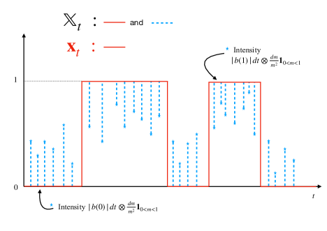
Figure 2.1. Sketch of the two limiting processes. The hidden Markov pure jump process ${\mathbf{x}}$ is in red, and the set-valued spike process ${\mathbb{X}}$ is in blue.

Such convergences were established thanks to a convenient (but fictitious) coupling of the processes $\left(\pi^{\gamma}\ ;\ \gamma>0\right)$ for different $\gamma>0$. In contrast, the filtering problem has a natural coupling for different $\gamma>0$ which is given by the observation equation (1.1). In this context, let us state a small adaptation of the theorem:

Theorem 2.2 (Variant of the Main Theorem of [BCC⁺22]).

There is a two-faceted convergence.

1. In the $\mathbb{L}^{0}$ topology and in probability, we have the following convergence :

   $$\left(\pi^{\gamma}_{t}\ ;0\leq t\leq H\right)\stackrel{{\scriptstyle\gamma\rightarrow\infty}}{{\longrightarrow}}\left({\mathbf{x}}_{t}\ ;0\leq t\leq H\right)\ .$$

   Equivalently, that is to say

   $$\forall\varepsilon>0,\quad\lim_{\gamma\rightarrow\infty}{\mathbb{P}}\left({\rm d}_{\mathbb{L}}(\pi^{\gamma},{\mathbf{x}})>\varepsilon\right)=0\ .$$

   Here ${\mathbf{x}}_{0}\in\{0,1\}$ is Bernoulli distributed with parameter $\pi^{\gamma}_{0}$ the initial condition of $\pi^{\gamma}$.
   

2. In the Hausdorff topology for graphs and in law, we have that the graph of $\left(\pi^{\gamma}_{t}\ ;0\leq t\leq H\right)$ converges to a spike process ${\mathbb{X}}=\bigsqcup_{t\in[0,H]}(\{t\}\times{\mathbb{X}}_{t})$ described by Fig. 2.1.
   

3. In the Hausdorff topology for graphs and in law, we have that the graph of $\hat{\mathbf{x}}^{\gamma}=\left(\hat{\mathbf{x}}^{\gamma}_{t}\ ;0\leq t\leq H\right)$, defined by Eq. (1.2), converges to another singular random closed set $\hat{\mathbb{X}}=\bigsqcup_{t\in[0,H]}(\{t\}\times\hat{\mathbb{X}}_{t})$ where

   $$\hat{{\mathbb{X}}}_{t}=\{0,1\}\mathds{1}_{\{{\mathbb{X}}_{t}\cap[0,\frac{1}{2})\neq\emptyset,{\mathbb{X}}_{t}\cap(\frac{1}{2},1]\neq\emptyset\}}+\{0\}\mathds{1}_{\{{\mathbb{X}}_{t}\subset[0,\frac{1}{2})\}}+\{1\}\mathds{1}_{\{{\mathbb{X}}_{t}\subset(\frac{1}{2},1]\}}\ .$$

Notice that the first convergence is in the weaker Lebesgue-type topology and holds in probability i.e. on the same probability space. The second and third convergences are in the stronger uniform-type topology, however they only hold in law.

Pointers to the proof.

The second point is indeed a direct corollary of [BCC⁺22] since almost sure convergence after a coupling implies convergence in law, regardless of the coupling. Although this coupling will be used in the paper further down the road, the reader should not give it much thought for the moment.

The third point is also immediate modulo certain subtleties. Recalling that $\hat{\mathbf{x}}_{t}^{\gamma}=\mathds{1}_{\{\pi_{t}^{\gamma}>\frac{1}{2}\}}$ and that the graph of $\pi^{\gamma}$ converges to the random closed set ${\mathbb{X}}$, it suffices to apply the Mapping Theorem [Bil13, Theorem 2.7]. Indeed, a spike ${\mathbb{X}}_{t}\subset[0,1]$ is mapped to either $\{0\}$, $\{1\}$ or $\{0,1\}$ when examining the range of the indicator $\mathds{1}_{\cdot>\frac{1}{2}}$ on ${\mathbb{X}}_{t}$. However, when invoking the Mapping Theorem, one needs to check that discontinuity points of the map $\mathds{1}_{\cdot>\frac{1}{2}}$ have measure zero for the law of ${\mathbb{X}}$. This is indeed true since there are no spikes of height $\frac{1}{2}$ almost surely.

The first point, although simpler and intuitive, does not come from [BCC⁺22]. In the case of filtering, the process ${\mathbf{x}}$ is intrinsically defined, and we require the use of the speficic coupling given by the additive model (1.1). Let us show how the result is reduced to a single claim. The result is readily obtained from the Markov inequality and the $L^{1}(\Omega)$ convergence:

$$\lim_{\gamma\rightarrow\infty}{\mathbb{E}}\ {\rm d}_{\mathbb{L}}\left(\pi^{\gamma},{\mathbf{x}}\right)=0\ .$$

The above convergence itself only requires the definition of ${\rm d}_{\mathbb{L}}$ in Eq. (2.6), Lebesgue’s dominated convergence theorem and the claim

$$\forall t>0,\quad\lim_{\gamma\rightarrow\infty}{\mathbb{E}}\left|\pi_{t}^{\gamma}-{\mathbf{x}}_{t}\right|^{2}=0\ .$$ (2.8)

In order to prove Claim (2.8), recall that by definition $\pi_{t}^{\gamma}$ is a conditional expectation:

$$\pi_{t}^{\gamma} =\ {\mathbb{P}}\left({\bf x}_{t}=1\ |\ \left({\bf y}^{\gamma}_{s}\right)_{s\leq t}\right)$$

$$=\textrm{argmin}_{c\in{\mathcal{F}}_{t}^{{\mathbf{y}}}}{\mathbb{E}}(\mathds{1}_{{\mathbf{x}}_{t}=1}-c)^{2}$$

$$=\textrm{argmin}_{c\in{\mathcal{F}}_{t}^{{\mathbf{y}}}}{\mathbb{E}}({\mathbf{x}}_{t}-c)^{2}\ .$$

At this stage, let $\varepsilon>0$ and let us introduce the process $z^{\varepsilon}=(z^{\varepsilon}_{t}\ ;\ t\geq\varepsilon)$ defined for all $t\geq\varepsilon$ by

$$z^{\varepsilon}_{t}=\frac{1}{\varepsilon}\int_{t-\varepsilon}^{t}d{\mathbf{y}}_{s}^{\gamma}\ .$$

This process is clearly $({\mathcal{F}}_{t}^{{\mathbf{y}}})_{t\geq\varepsilon}$ adapted, so for all $t\geq\varepsilon$, by definition of $\pi_{t}^{\gamma}$

$${\mathbb{E}}\left|\pi_{t}^{\gamma}-{\mathbf{x}}_{t}\right|^{2}\leq \ {\mathbb{E}}\left|z^{\varepsilon}_{t}-{\mathbf{x}}_{t}\right|^{2}$$

$$= \ {\mathbb{E}}\left|\frac{1}{\varepsilon}\int_{t-\varepsilon}^{t}d{\mathbf{y}}_{s}^{\gamma}-{\mathbf{x}}_{t}\right|^{2}$$

$$= \ {\mathbb{E}}\left|\frac{1}{\varepsilon}\int_{t-\varepsilon}^{t}{\mathbf{x}}_{s}ds-{\mathbf{x}}_{t}+\frac{1}{\varepsilon\sqrt{\gamma}}\int_{t-\varepsilon}^{t}dB_{s}\right|^{2}$$

$$\leq \ 2{\mathbb{E}}\left|\frac{1}{\varepsilon}\int_{t-\varepsilon}^{t}{\mathbf{x}}_{s}ds-{\mathbf{x}}_{t}\right|^{2}+2{\mathbb{E}}\left|\frac{1}{\varepsilon\sqrt{\gamma}}\int_{t-\varepsilon}^{t}dB_{s}\right|^{2}$$

$$= \ 2{\mathbb{E}}\left|\frac{1}{\varepsilon}\int_{t-\varepsilon}^{t}({\mathbf{x}}_{s}-{\mathbf{x}}_{t})ds\right|^{2}+\frac{2}{\varepsilon\gamma}$$

$$\leq \ 2{\mathbb{E}}\left|\frac{1}{\varepsilon}\int_{t-\varepsilon}^{t}\mathds{1}_{\{{\mathbf{x}}_{s}\neq{\mathbf{x}}_{t}\}}ds\right|^{2}+\frac{2}{\varepsilon\gamma}$$

$$\leq \ 2{\mathbb{P}}\left({\mathbf{x}}\textrm{ jumps at least one time during }[t-\varepsilon,t]\right)+\frac{2}{\varepsilon\gamma}\ .$$

Note that we have used that for $\varepsilon\leq s\leq t,$

$$\{{\mathbf{x}}_{s}\neq{\mathbf{x}}_{t}\}\subset\{{\mathbf{x}}\textrm{ jumps at least one time during }[t-\varepsilon,t]\}.$$

Taking $\gamma\rightarrow\infty$ then $\varepsilon\rightarrow 0$ proves Claim (2.8). ∎

We can now formally state the question of interest:

Question 2.3.

For different regimes of $\delta=\delta_{\gamma}$ and $\gamma$, how do the spikes behave in the stochastic process (1.4)? Basically, we need an understanding of the tradeoff between spiking and smoothing. The intuition is that there are two regimes:

• The slow feedback regime: the smoothing window $\delta$ is large enough so that the optimal estimator $\pi^{\delta,\gamma}$ correctly estimates the hidden process ${\mathbf{x}}$.

• The fast feedback regime: the smoothing window $\delta$ is too small so that $\pi^{\delta,\gamma}$ does not correctly estimate the hidden process ${\mathbf{x}}$. One does observe the effect of spikes.

2.3. Main Theorem

Our finding is that there is sharp transition between the slow feedback regime and the fast feedback regime:

Theorem 2.4 (Main theorem).

As long as $\delta_{\gamma}\rightarrow 0$, we have the convergence in the $\mathbb{L}^{0}$ topology and in probability, as in the first item of Theorem 2.2:

$$\left(\pi^{\delta_{\gamma},\gamma}_{t}\ ;0\leq t\leq H\right)\stackrel{{\scriptstyle\gamma\rightarrow\infty}}{{\longrightarrow}}\left({\mathbf{x}}_{t}\ ;0\leq t\leq H\right)\ .$$ (2.9)

However, in the stronger topologies, there exists a sharp transition when writing:

$$\delta_{\gamma}=C\frac{\log\gamma}{\gamma}\ .$$

The following convergences hold in the Hausdorff topology on graphs in $[0,H]\times[0,1]$.

• (Fast feedback regime) If $C<2$, smoothing does not occur and we have convergence in law to the spike process:

  $$\lim_{\gamma\rightarrow\infty}\pi^{\delta_{\gamma},\gamma}={\mathbb{X}}\ .$$

• (Slow feedback regime) If $C>2$, smoothing occurs and we have convergence:

  $$\lim_{\gamma\rightarrow\infty}\pi^{\delta_{\gamma},\gamma}={\mathbf{x}}\ .$$

  This convergence holds equivalently for the usual $M_{2}$ Skorohod topology and for the Hausdorf topology on graphs.

Sketch of proof.

The proof given in Theorem 2.2 carries verbatim to proving (2.9). We will not be repeat it.

For the rest of the paper, since we only need to establish convergences in law, for the Hausdorff topology, it is more convenient to prove almost sure convergence for any coupling of the Wiener process $B=B^{\gamma}$ in Eq. (1.1). Equivalently, we can choose a coupling of $W=W^{\gamma}$, which we take as the Dambis-Dubins-Schwarz coupling of [BCC⁺22]. In that setting, we know that $\lim_{\gamma\rightarrow\infty}\pi^{\gamma}={\mathbb{X}}$.

In Section 3, we give in Proposition 3.1 a derivation of $\pi^{\delta_{\gamma},\gamma}$ in terms of the process $\pi^{0,\gamma}=\pi^{\gamma}=\left(\pi^{\gamma}_{t}\ ;\ t\geq 0\right)$. This will allow for a informal discussion explaining the phenomenon via a certain damping factor $\int_{s}^{t}a^{\gamma}$.

Before the core of the proof, we do some preparatory work in Section 4, where we prove that only the damping term needs to be analyzed and give a trajectorial decomposition.

The core of the proof is in Section 5. The proof of the first statement is in Subsection 5.3, while the proof of the second statement is in Subsection 5.4. ∎

2.4. Further remarks

On the transition: Without much change in the proof, one can consider $C=C_{\gamma}$ depending on $\gamma$. In that setting, the fast feed-back regime and the slow feed-back regime correspond respectively to

$$\limsup_{\gamma\rightarrow\infty}C_{\gamma}<2\textrm{ and }\liminf_{\gamma\rightarrow\infty}C_{\gamma}>2\ .$$

Furthermore, one could ask the question of what happens at exactly the transition and if there is possible zooming around the constant $C_{\gamma}=2$. We chose to consider the matter beyond the scope of the paper.

Away from the transition: Because of the monotonicity of the damping, as a positive integral, one can easily deduce what is happening if $C_{\gamma}$ remains away from the threshold constant $2$.

Is the convergence to the spike process only in law as $\gamma\rightarrow\infty$? Not in probability or almost surely? This point is rather subtle and we mainly choose to sweep it under the rug. Nevertheless, let us make the following comment. In the context of filtering, the spikes correspond to exceptionally fast points of the Brownian motion appearing in the noise $B=B^{\gamma}$. Let us assume that for some (unphysical) reason, $B^{\gamma}$ remains the same i.e. one can perfectly tune the strength of the noise at will. For different $\gamma$, the spikes appear as functionals of the Brownian motion $B$ at different scales. Therefore, we argue that there is no hope for obtaining a natural trajectorial limit to the spike process as $\gamma\rightarrow\infty$.

On the general Wonham-Shiryaev filter: It is a natural question to generalize our Main Theorem to the Wonham-Shiryaev filter with $n$ states from Eq. (2.1). However, the mathematical technology dealing with the spiking phenomenon in a multi-dimensional setting is an open problem still under investigation.

3. Smoothing transform

We shall express the equation satisfied by (1.4). The general theory is given in [Lip01, Chapter 9]. For $s\leq t$ we write:

$$\pi_{s,t}^{\gamma}:=\pi_{s,t}^{\gamma}(1)=\ {\mathbb{P}}\left({\mathbf{x}}_{s}=1\ |\ \left({\bf y}^{\gamma}_{s}\right)_{s\leq t}\right)\ .$$

and, in particular, the process defined by Eq. (1.4) is such that

$$\pi^{\delta_{\gamma},\gamma}_{t}=\pi^{\gamma}_{t-\delta_{\gamma},t}.$$

Proposition 3.1.

For any $0\leq s\leq t$ we have that

$$\pi_{s,t}^{\gamma}=\pi_{t}^{\gamma}\ e^{-\int_{s}^{t}a_{u}^{\gamma}du}+\int_{s}^{t}\lambda_{1,0}\frac{\pi^{\gamma}_{u}}{1-\pi^{\gamma}_{u}}e^{-\int_{s}^{u}a^{\gamma}_{v}dv}du$$ (3.1)

where the instantaneous damping term is given by

$$a^{\gamma}_{u}:=a(\pi^{\gamma}_{u})=\lambda_{1,0}\frac{\pi^{\gamma}_{u}}{1-\pi^{\gamma}_{u}}+\lambda_{0,1}\frac{1-\pi^{\gamma}_{u}}{\pi^{\gamma}_{u}}\ .$$ (3.2)

Proof.

To simplify notation, during the proof we forget the dependence in $\gamma$ and denote, for all $\alpha\in\{0,1\}$

$$\Pi_{s,t}(\alpha):=\ {\mathbb{P}}\left({\mathbf{x}}_{s}=\alpha\ |\ \left({\bf y}^{\gamma}_{s}\right)_{s\leq t}\right)\ ,\quad\Pi_{t}(\alpha):=\ {\mathbb{P}}\left({\mathbf{x}}_{t}=\alpha\ |\ \left({\bf y}^{\gamma}_{s}\right)_{s\leq t}\right)\ .$$

Thanks to [Lip01, Theorem 9.5], we have:

$$\partial_{s}\Pi_{s,t} =-\Pi_{s}{\mathcal{L}}\left[\tfrac{\Pi_{s,t}}{\Pi_{s}}\right]+\tfrac{\Pi_{s,t}}{\Pi_{s}}{\mathcal{L}}^{*}\left[\Pi_{s}\right]\ ,$$

which we will specialize to the point $\alpha=1$. Note that:

$$\Pi_{s,t}(1) =\pi_{s,t}\ ,$$

$${\mathcal{L}}\left[\tfrac{\Pi_{s,t}}{\Pi_{s}}\right](1) =\lambda_{1,0}\tfrac{\Pi_{s,t}(0)}{\Pi_{s}(0)}-\lambda_{1,0}\tfrac{\Pi_{s,t}(1)}{\Pi_{s}(1)}$$

$$=\lambda_{1,0}\left(\tfrac{1-\pi_{s,t}}{1-\pi_{s}}-\tfrac{\pi_{s,t}}{\pi_{s}}\right)\ ,$$

$${\mathcal{L}}^{*}\left[\Pi_{s}\right](1) =\lambda_{0,1}\Pi_{s}(0)-\lambda_{1,0}\Pi_{s}(1)$$

$$=\lambda_{0,1}\left(1-\pi_{s}\right)-\lambda_{1,0}\pi_{s}\ .$$

Resuming the computation:

$$\partial_{s}\pi_{s,t} =-\pi_{s}\lambda_{1,0}\left(\frac{1-\pi_{s,t}}{1-\pi_{s}}-\frac{\pi_{s,t}}{\pi_{s}}\right)+\frac{\pi_{s,t}}{\pi_{s}}\left(\lambda_{0,1}\left(1-\pi_{s}\right)-\lambda_{1,0}\pi_{s}\right)$$

$$=-\lambda_{1,0}\frac{\pi_{s}}{1-\pi_{s}}-\pi_{s}\lambda_{1,0}\left(\frac{-\pi_{s,t}}{1-\pi_{s}}-\frac{\pi_{s,t}}{\pi_{s}}\right)+\frac{\pi_{s,t}}{\pi_{s}}\left(\lambda_{0,1}\left(1-\pi_{s}\right)-\lambda_{1,0}\pi_{s}\right)$$

$$=-\lambda_{1,0}\frac{\pi_{s}}{1-\pi_{s}}+\pi_{s,t}\lambda_{1,0}\frac{1}{1-\pi_{s}}+\pi_{s,t}\left(\lambda_{0,1}\left(\frac{1}{\pi_{s}}-1\right)-\lambda_{1,0}\right)$$

$$=-\lambda_{1,0}\frac{\pi_{s}}{1-\pi_{s}}+\pi_{s,t}\left[\lambda_{1,0}\frac{\pi_{s}}{1-\pi_{s}}+\lambda_{0,1}\frac{1-\pi_{s}}{\pi_{s}}\right]$$

$$=-\lambda_{1,0}\frac{\pi_{s}}{1-\pi_{s}}+\pi_{s,t}a_{s}\ .$$

One recognizes an ordinary differential equation in the variable $s$, with $s\leq t$. Upon solving, we have:

$$\pi_{s,t}=\pi_{t}\ e^{-\int_{s}^{t}a_{u}du}+\int_{s}^{t}\lambda_{1,0}\frac{\pi_{u}}{1-\pi_{u}}e^{-\int_{s}^{u}a_{v}dv}du.$$

This is exactly the result. ∎

Remark 3.2.

Recall Eq. (3.2). Notice the exact derivative:

$$\int_{s}^{t}\lambda_{0,1}\frac{1-\pi_{u}}{\pi_{u}}e^{-\int_{s}^{u}a_{v}dv}du+\int_{s}^{t}\lambda_{1,0}\frac{\pi_{u}}{1-\pi_{u}}e^{-\int_{s}^{u}a_{v}dv}du=\int_{s}^{t}a_{u}e^{-\int_{s}^{u}a_{v}dv}du=1-e^{-\int_{s}^{t}a_{u}du}\ .$$

Corollary 3.3.

We have a dual expression:

$$1-\pi^{\gamma}_{s,t}=(1-\pi^{\gamma}_{t})\ e^{-\int_{s}^{t}a^{\gamma}_{u}du}+\int_{s}^{t}\lambda_{0,1}\frac{1-\pi^{\gamma}_{u}}{\pi^{\gamma}_{u}}e^{-\int_{s}^{u}a^{\gamma}_{v}dv}du\ .$$

We have:

$$\begin{split}\pi^{\gamma}_{s,t}=&\ {\mathbf{x}}_{t}+(\pi^{\gamma}_{t}-{\mathbf{x}}_{t})e^{-\int_{s}^{t}a^{\gamma}_{u}du}-{\mathbf{x}}_{t}(1-e^{-\int_{s}^{t}a^{\gamma}_{u}du})+\int_{s}^{t}\lambda_{1,0}\frac{\pi^{\gamma}_{u}}{1-\pi^{\gamma}_{u}}e^{-\int_{s}^{u}a^{\gamma}_{v}dv}du\\ =&\ {\mathbf{x}}_{t}+(\pi^{\gamma}_{t}-{\mathbf{x}}_{t})e^{-\int_{s}^{t}a^{\gamma}_{u}du}+(1-{\mathbf{x}}_{t})(1-e^{-\int_{s}^{t}a^{\gamma}_{u}du})-\int_{s}^{t}\lambda_{0,1}\frac{1-\pi^{\gamma}_{u}}{\pi^{\gamma}_{u}}e^{-\int_{s}^{u}a^{\gamma}_{v}dv}du\ .\end{split}$$ (3.3)

In a single expression, one can write:

$$\pi_{s,t}^{\gamma}= \ {\mathbf{x}}_{t}+(\pi^{\gamma}_{t}-{\mathbf{x}}_{t})e^{-\int_{s}^{t}a^{\gamma}_{u}du}$$ (3.4)

$$\ +\mathds{1}_{\{{\mathbf{x}}_{t}=0\}}\int_{s}^{t}\lambda_{1,0}\frac{\pi_{u}^{\gamma}}{1-\pi^{\gamma}_{u}}e^{-\int_{s}^{u}a^{\gamma}_{v}dv}du-\mathds{1}_{\{{\mathbf{x}}_{t}=1\}}\int_{s}^{t}\lambda_{0,1}\frac{1-\pi^{\gamma}_{u}}{\pi_{u}^{\gamma}}e^{-\int_{s}^{u}a^{\gamma}_{v}dv}du\ .$$

Proof.

The dual expression is obvious by symmetry or using the following exact derivative from Remark 3.2:

$$\pi_{s,t}= \pi_{t}\ e^{-\int_{s}^{t}a_{u}du}+\int_{s}^{t}a_{u}e^{-\int_{s}^{u}a_{v}dv}du-\int_{s}^{t}\lambda_{0,1}\frac{1-\pi_{u}}{\pi_{u}}e^{-\int_{s}^{u}a_{v}dv}du$$

$$= \pi_{t}\ e^{-\int_{s}^{t}a_{u}du}+1-e^{-\int_{s}^{t}a_{u}du}-\int_{s}^{t}\lambda_{0,1}\frac{1-\pi_{u}}{\pi_{u}}e^{-\int_{s}^{u}a_{v}dv}du\ .$$

For the final expressions in Eq. (3.3), write:

$$\pi_{s,t}= \pi_{t}\ e^{-\int_{s}^{t}a_{u}du}+\int_{s}^{t}\lambda_{1,0}\frac{\pi_{u}}{1-\pi_{u}}e^{-\int_{s}^{u}a_{v}dv}du$$

$$= {\mathbf{x}}_{t}+\left(\pi_{t}-{\mathbf{x}}_{t}\right)\ e^{-\int_{s}^{t}a_{u}du}-{\mathbf{x}}_{t}\left(1-e^{-\int_{s}^{t}a_{u}du}\right)+\int_{s}^{t}\lambda_{1,0}\frac{\pi_{u}}{1-\pi_{u}}e^{-\int_{s}^{u}a_{v}dv}du\ .$$

This yields the first one. The second is obtained via Remark 3.2. ∎

Intuition: Whenever there is no jump on $[t-\delta_{\gamma},t]$, all spikes are of size $<1$. If $\pi_{t}^{\gamma}$ is collapsing on $0$, then:

$$\int_{t-\delta_{\gamma}}^{t}\lambda_{1,0}\frac{\pi^{\gamma}_{u}}{1-\pi^{\gamma}_{u}}\exp\left({-\int_{t-\delta^{\gamma}}^{u}a^{\gamma}_{v}dv}\right)du=o(1)$$

and reciprocally when the collapse is on $1$. From the previous corollary, we thus have:

$$\pi_{t}^{\delta_{\gamma},\gamma}= {\mathbf{x}}_{t}+(\pi^{\gamma}_{t}-{\mathbf{x}}_{t})e^{-D_{t}^{\gamma}}+o_{\gamma}(1)$$

where the damping term is given by

$$D_{t}^{\gamma}=\int_{t-\delta_{\gamma}}^{t}a_{u}^{\gamma}\ du=\int_{t-\delta_{\gamma}}^{t}\left\{\lambda_{1,0}\tfrac{\pi^{\gamma}_{u}}{1-\pi^{\gamma}_{u}}+\lambda_{0,1}\tfrac{1-\pi^{\gamma}_{u}}{\pi^{\gamma}_{u}}\right\}\ du\ .$$ (3.5)

Assuming that the damping term $D^{\gamma}$ converges to some limiting process $D$ we expect that

$$\lim_{\gamma\rightarrow\infty}\pi_{t}^{\delta_{\gamma},\gamma}={\mathbf{x}}_{t}+({\mathbb{X}}_{t}-{\mathbf{x}}_{t})e^{-D_{t}}\ .$$ (3.6)

Above, the limiting graph is defined by its slice at time $t$, which is given by ${\mathbb{X}}_{t}$ translated by $-{\mathbf{x}}_{t}$ and then rescaled by a factor $e^{-D_{t}}$, and then translated by ${\mathbf{x}}_{t}$ again.

Informally, there are three cases:

• Slow feedback: $D=\infty$ and therefore

  $$\lim_{\gamma\rightarrow\infty}\pi_{t}^{\delta_{\gamma},\gamma}={\mathbf{x}}_{t}\ .$$

• Transitory regime: $D$ is non-trivial and therefore

  $$\lim_{\gamma\rightarrow\infty}\pi_{t}^{\delta_{\gamma},\gamma}={\mathbf{x}}_{t}+({\mathbb{X}}_{t}-{\mathbf{x}}_{t})e^{-D_{t}}\ ,$$

  with $D$ having a statistic which needs to be analyzed. This analysis is beyond the scope of this paper as mentioned in Subsection 2.4.

• Fast feedback: $D=0$ and therefore

  $$\lim_{\gamma\rightarrow\infty}\pi_{t}^{\delta_{\gamma},\gamma}={\mathbb{X}}_{t}\ .$$

4. Reduction to the control of the damping term

Here we prove a useful intermediary step, which informally says that:

$$\pi_{t}^{\delta_{\gamma},\gamma}\approx{\mathbf{x}}_{t}+\left(\pi^{\gamma}_{t}-{\mathbf{x}}_{t}\right)e^{-D_{t}^{\gamma}}.$$ (4.1)

This is the combination of two simplifying facts:

• During jumps, Hausdorff proximity is guaranteed. Indeed, the graph of the spike process and ${\mathbf{x}}$ are very close in the Hausdorff sense and they take the full segment $[0,1]$ vertically. Thus no matter where $\pi_{s,t}$ is, the Hausdorff distance will be small.

• If $|t-s|\rightarrow 0$, away from jumps, the remainder benefits from smoothing.

Once this is established, we only need to control the damping term $D^{\gamma}$ outside from small spikes. Let us now make these informal statements rigorous.

Let us start with few notations and conventions. If $f:t\in I\mapsto f_{t}\in[0,1]$ is a function defined on a closed subset $I$ of $[0,H]$, we denote by ${\mathcal{G}}(f)$ its graph:

• If $f$ is a continuous function continuous then we define its graph by

  $${\mathcal{G}}(f)=\{(t,f_{t})\;;\;t\in I\}.$$

• If $f$ is a càdlàg function then, by denoting by ${\mathfrak{d}}_{f}$ the set of discontinuous points of $f$, we define its graph by

  $${\mathcal{G}}(f)=\{(t,f_{t})\;;\;t\in I\backslash{\mathfrak{d}}_{f}\}\cup_{t\in{\mathfrak{d}}_{f}}(\{t\}\times[0,1])\ .$$

We recall that the slice at time $t$ of a graph $\mathcal{G}$ is denoted by $\mathcal{G}_{t}$. In order to simplify the notations, we write ${\mathcal{G}}^{\gamma}={\mathcal{G}}(\pi^{\delta_{\gamma},\gamma})$ for the graph induced by the process of interest (which has contiunous trajectories). And we write ${\mathcal{G}}^{\infty}={\mathcal{G}}^{C,\infty}$ is the candidate for the limiting graph, either the completed graphs ${\mathbb{X}}$ (if $C<2$) or ${\mathcal{G}}({\mathbf{x}})$ (if $C>2$). By the convention above, in the definition of ${\mathcal{G}}({\mathbf{x}})$, the graph induced by the process ${\mathbf{x}}$, we add a vertical bar when there is a jump. We define also ${\mathcal{G}}^{\gamma,\circ}$ the graph whose slice at time $t\in[\delta_{\gamma},H]$ is given by

$${\mathcal{G}}^{\gamma,\circ}_{t}\ :=\ {\mathcal{G}}_{t}({\mathbf{x}})+(\pi^{\gamma}_{t}-{\mathbf{x}}_{t})e^{-D_{t}^{\gamma}}$$ (4.2)

and the empty set if $t\in(0,\delta_{\gamma})$. Observe in particular that $\mathcal{G}^{\gamma,\circ}$ contains the vertical bar $[0,1]$ when there is a jump of ${\mathbf{x}}$. We define also the graph ${\mathcal{G}}^{\gamma,\diamond}$ whose slice at time $t\in[\delta_{\gamma},H]$ is given by

$${\mathcal{G}}_{t}^{\gamma,\diamond}:={\mathcal{G}}_{t-\delta_{\gamma}}({\mathbf{x}})+(\pi_{t-\delta_{\gamma}}^{\gamma}-{\mathbf{x}}_{t-\delta_{\gamma}})e^{-D_{t}^{\gamma}}\ .$$ (4.3)

The following formalises the informal statement of Eq. (4.1):

Proposition 4.1.

Consider a coupling such that almost surely

$$\lim_{\gamma\to\infty}{\rm d}_{\mathbb{L}}(\pi^{\gamma},{\mathbf{x}})=0\ ,$$ (4.4)

$$\lim_{\gamma\to\infty}{\rm d}_{\mathbb{H}}({\mathcal{G}}(\pi^{\gamma}),\mathbb{X})=0\ .$$ (4.5)

Then, almost surely:

$$\lim_{\gamma\rightarrow\infty}{\rm d}_{\mathbb{L}}(\pi^{\delta_{\gamma},\gamma},{\mathbf{x}}) =0\ ,$$ (4.6)

$$\lim_{\gamma\rightarrow\infty}{\rm d}_{\mathbb{H}}({\mathcal{G}}^{\gamma},{\mathcal{G}}^{\gamma,\circ}) =0\ .$$ (4.7)

Proof.

Let $J_{1},J_{2},\dots$ be the successive jump times of ${\mathbf{x}}$ and denote by $N=\sup\{i\geq 1\;;\;J_{i}\leq H\}<\infty$ the number of jumps in the time interval $[0,H]$. It is easy to prove that

$$\lim_{\eta\to 0}\mathbb{P}\left(\;\inf_{i\leq N}|J_{i}-J_{i-1}|\geq 2\eta\right)=1\ .$$

On the event $\Omega_{\eta}=\{\inf_{i\leq N}|J_{i}-J_{i-1}|\geq 2\eta\}$ we define then the compact sets for $\varepsilon<\eta$:

$$\begin{split}&J_{\varepsilon}:=\cup_{i=1}^{N}[J_{i}-\varepsilon,J_{i}+\varepsilon]\ ,\quad J_{\varepsilon}^{\square}:=J_{\varepsilon}\times[0,1]\ ,\\ &K_{\varepsilon}:=[0,H]\backslash\cup_{i=1}^{N}(J_{i}-\varepsilon,J_{i}+\varepsilon)\ ,\quad K_{\varepsilon}^{\square}:=K_{\varepsilon}\times[0,1]\ .\end{split}$$

By Theorem 1.12.15 in [Bar06] we have that for any compact subsets $A,B,C,D$ of $[0,H]\times[0,1]$,

$${\rm d}_{{\mathbb{H}}}(A\cup B,C\cup D)\leq\max\left\{{\rm d}_{\mathbb{H}}(A,C),{\rm d}_{\mathbb{H}}(B,D)\right\}\ .$$ (4.8)

Since ${\mathcal{G}}^{\gamma}=({\mathcal{G}}^{\gamma}\cap J_{\varepsilon}^{\square})\cup({\mathcal{G}}^{\gamma}\cap K_{\varepsilon}^{\square})$ (and similarly for $\mathcal{G}^{\gamma}$ replaced by ${\mathcal{G}}^{\gamma,\circ}$) it follows that

$${\rm d}_{\mathbb{H}}({\mathcal{G}}^{\gamma},{\mathcal{G}}^{\gamma,\circ}) \leq{\rm d}_{\mathbb{H}}\left({\mathcal{G}}^{\gamma}\cap J_{\varepsilon}^{\square},{\mathcal{G}}^{\gamma,\circ}\cap J_{\varepsilon}^{\square}\right)+{\rm d}_{\mathbb{H}}\left({\mathcal{G}}^{\gamma}\cap K_{\varepsilon}^{\square},{\mathcal{G}}^{\gamma,\circ}\cap K_{\varepsilon}^{\square}\right)\ .$$

Hence we only have to prove that on each event $\Omega_{\eta}$:

$$\lim_{\varepsilon\rightarrow 0}\limsup_{\gamma\to\infty}{\rm d}_{\mathbb{H}}\left({\mathcal{G}}^{\gamma}\cap J_{\varepsilon}^{\square},{\mathcal{G}}^{\gamma,\circ}\cap J_{\varepsilon}^{\square}\right)=0\ ,$$ (4.9)

and

$$\lim_{\varepsilon\rightarrow 0}\limsup_{\gamma\to\infty}{\rm d}_{\mathbb{H}}\left({\mathcal{G}}^{\gamma}\cap K_{\varepsilon}^{\square},{\mathcal{G}}^{\gamma,\circ}\cap K_{\varepsilon}^{\square}\right)=0\ .$$ (4.10)

Step 1: Hausdorff proximity away from the jump times: proof of Eq. (4.10)

Step 1.1: Spikes are of size less than $1-\varepsilon$ with high probability.

Let $M^{*}$ be the largest length of a spike:

$$M^{*}:=\max_{t\in[0,H]}\max_{y\in{\mathbb{X}}_{t}\backslash{\mathcal{G}}_{t}({\mathbf{x}})}\left\{\left|y\right|\mathds{1}_{{\mathbf{x}}_{t}=0},(1-\left|y\right|)\mathds{1}_{{\mathbf{x}}_{t}=1}\right\}\ .$$ (4.11)

From the explicit description of the law of ${\mathbb{X}}$, $M^{*}$ is the maximum decoration of a Poisson process on $[0,H]\times[0,1]$ with intensity

$$\left(p\mathds{1}_{\{{\mathbf{x}}_{t}=0\}}+(1-p)\mathds{1}_{\{{\mathbf{x}}_{t}=1\}}\right)\lambda dt\otimes\frac{dm}{m^{2}}\ .$$

Upon conditioning on the process ${\mathbf{x}}$, and considering the definition of a Poisson process [Kin92, §2.1], notice that that the number of points falling inside $[0,H]\times(1-\eta,1)$ is a Poisson random variable with parameter

$$\int_{[0,H]\times(1-\eta,1)}\left(p\mathds{1}_{\{{\mathbf{x}}_{t}=0\}}+(1-p)\mathds{1}_{\{{\mathbf{x}}_{t}=1\}}\right)\lambda dt\otimes\frac{dm}{m^{2}}\ .$$

As such the event $\{M^{*}\leq 1-\eta\}$ corresponds to having this Poisson random variable being zero, so that:

$$\begin{split}&{\mathbb{P}}\left(M^{*}\leq 1-\eta\right)\\ =&\ {\mathbb{E}}\exp\left(-\int_{[0,H]\times(1-\eta,1)}\left(p\mathds{1}_{\{{\mathbf{x}}_{t}=0\}}+(1-p)\mathds{1}_{\{{\mathbf{x}}_{t}=1\}}\right)\lambda dt\otimes\frac{dm}{m^{2}}\right)\\ =&\ {\mathbb{E}}\exp\left(-\lambda\left(1/(1-\eta)-1\right)\int_{0}^{H}\left(p\mathds{1}_{\{{\mathbf{x}}_{t}=0\}}+(1-p)\mathds{1}_{\{{\mathbf{x}}_{t}=1\}}\right)dt\right)\\ =&{\mathbb{E}}\exp\left(-\frac{\lambda\eta}{1-\eta}\int_{0}^{H}\left(p\mathds{1}_{\{{\mathbf{x}}_{t}=0\}}+(1-p)\mathds{1}_{\{{\mathbf{x}}_{t}=1\}}\right)dt\right)\\ \geq&\exp\left(-\frac{\lambda\eta}{1-\eta}H\max(p,1-p)\right)\ .\end{split}$$ (4.12)

As such, it is clear that from Eq. (4.12) that

$$\lim_{\eta\to 0}\mathbb{P}(M^{*}\leq 1-\eta)=1\ .$$

We observe now, by definition of Hausdorff distance, that for any $t\in K_{\varepsilon}$ and $u\in[t-\delta_{\gamma},t]$ there exists $s\in[0,H]$ and $x\in\mathbb{X}_{s}$ such that

$$\|(s,x)-(u,\pi_{u}^{\gamma})\|^{2}=|s-u|^{2}+|x-\pi_{u}^{\gamma}|^{2}\leq{\rm d}^{2}_{{\mathbb{H}}}\left({\mathcal{G}}(\pi^{\gamma}),\mathbb{X}\right)\ .$$

From the definition of $M^{*}$, it implies that

$$\sup_{\begin{subarray}{c}t\in K_{\varepsilon}\\ {{\mathbf{x}}}_{t}=0\end{subarray}}\;\sup_{u\in[t-\delta_{\gamma},t]}\pi_{u}^{\gamma}\leq M^{*}+{\rm d}_{{\mathbb{H}}}\left({\mathcal{G}}(\pi^{\gamma}),\mathbb{X}\right)$$ (4.13)

and

$$\begin{split}\inf_{\begin{subarray}{c}t\in K_{\varepsilon}\\ {{\mathbf{x}}}_{t}=1\end{subarray}}\;\inf_{u\in[t-\delta_{\gamma},t]}\pi_{u}^{\gamma}\geq(1-M^{*})-{\rm d}_{{\mathbb{H}}}\left({\mathcal{G}}(\pi^{\gamma}),\mathbb{X}\right)\ .\end{split}$$ (4.14)

Let us then denote the event

$$\Omega_{\eta}^{\prime}:=\Omega_{\eta}\cap\{M^{*}\leq 1-2\eta\}$$

which satisfies, $\liminf_{\eta\to 0}\mathbb{P}(\Omega_{\eta}^{\prime})=1$, and on which we have

$$\min\left(M_{0}^{\gamma},M_{1}^{\gamma}\right)\geq \ 2\eta-{\rm d}_{{\mathbb{H}}}\left({\mathcal{G}}(\pi^{\gamma}),\mathbb{X}\right)$$ (4.15)

where

$$M_{0}^{\gamma}:=\inf_{\begin{subarray}{c}t\in K_{\varepsilon}\\ {{\mathbf{x}}}_{t}=0\end{subarray}}\;\inf_{u\in[t-\delta_{\gamma},t]}1-\pi_{u}^{\gamma}\quad \text{and}\quad M_{1}^{\gamma}:=\inf_{\begin{subarray}{c}t\in K_{\varepsilon}\\ {{\mathbf{x}}}_{t}=1\end{subarray}}\;\inf_{u\in[t-\delta_{\gamma},t]}\pi_{u}^{\gamma}\ .$$

Notice in particular that:

$$\limsup_{\gamma\rightarrow\infty}\frac{1}{M_{0}^{\gamma}}+\frac{1}{M_{1}^{\gamma}}\leq\frac{1}{\eta}\ .$$ (4.16)

Step 1.2:

Recall Eq. (3.4). For $t\in[\delta_{\gamma},H]\backslash J_{\varepsilon}$, on the event ${\Omega}_{\eta}^{\prime}$, we have thanks to Eq. (4.15), that

$$\left|\pi_{t}^{\delta_{\gamma},\gamma}-\left({\mathbf{x}}_{t}+(\pi^{\gamma}_{t}-{\mathbf{x}}_{t})e^{-D_{t}^{\gamma}}\right)\right|$$

$$\leq \mathds{1}_{\{{\mathbf{x}}_{t}=0\}}\int_{t-\delta_{\gamma}}^{t}\lambda_{1,0}\frac{\pi_{u}^{\gamma}}{1-\pi^{\gamma}_{u}}du+\mathds{1}_{\{{\mathbf{x}}_{t}=1\}}\int_{t-\delta_{\gamma}}^{t}\lambda_{0,1}\frac{1-\pi^{\gamma}_{u}}{\pi_{u}^{\gamma}}du$$

$$\leq \ \left(\frac{1}{M_{0}^{\gamma}}+\frac{1}{M_{1}^{\gamma}}\right)\left(\mathds{1}_{\{{\mathbf{x}}_{t}=0\}}\int_{t-\delta_{\gamma}}^{t}\pi_{u}^{\gamma}du+\mathds{1}_{\{{\mathbf{x}}_{t}=1\}}\int_{t-\delta_{\gamma}}^{t}(1-\pi^{\gamma}_{u})du\right)$$

$$\stackrel{{\scriptstyle(*)}}{{=}} \ \left(\frac{1}{M_{0}^{\gamma}}+\frac{1}{M_{1}^{\gamma}}\right)\left(\mathds{1}_{\{{\mathbf{x}}_{t}=0\}}\int_{t-\delta_{\gamma}}^{t}(\pi_{u}^{\gamma}-{\mathbf{x}}_{u})du+\mathds{1}_{\{{\mathbf{x}}_{t}=1\}}\int_{t-\delta_{\gamma}}^{t}({\mathbf{x}}_{u}-\pi^{\gamma}_{u})du\right)$$

$$= \ \left(\frac{1}{M_{0}^{\gamma}}+\frac{1}{M_{1}^{\gamma}}\right)\int_{t-\delta_{\gamma}}^{t}\left|\pi_{u}^{\gamma}-{\mathbf{x}}_{u}\right|du$$

$$\leq \ \left(\frac{1}{M_{0}^{\gamma}}+\frac{1}{M_{1}^{\gamma}}\right)\delta_{\gamma}\ .$$

The step marked with (*) holds because there is no jump during $[t-\delta_{\gamma},t]$ for $t\in K_{\varepsilon}$ as soon as $\delta_{\gamma}<\varepsilon$. Taking limits and using Eq. (4.16), we conclude that:

$$\limsup_{\gamma\rightarrow\infty}\sup_{t\in K_{\varepsilon}}\left|\pi_{t}^{\delta_{\gamma},\gamma}-\left({\mathbf{x}}_{t}+(\pi^{\gamma}_{t}-{\mathbf{x}}_{t})e^{-D_{t}^{\gamma}}\right)\right|\leq \ \limsup_{\gamma\rightarrow\infty}\frac{\delta_{\gamma}}{\eta}=0\ .$$ (4.17)

This limit holds on $\Omega_{\eta}^{\prime}$ for all $\eta>0$. We have thus proven that away from jumps the Hausdorff distance tends to zero. This concludes the proof of Eq. (4.10).

Step 2: Proof of Eq. (4.6)

From the definition of the distance $d_{\mathbb{L}}$

$${\rm d}_{\mathbb{L}}(\pi^{\delta_{\gamma},\gamma},{\mathbf{x}})$$

$$= \ \int_{0}^{H}\left|\pi^{\delta_{\gamma},\gamma}_{t}-{\mathbf{x}}_{t}\right|dt$$

$$\leq \ 2\varepsilon N+\int_{K_{\varepsilon}}\left|\pi^{\delta_{\gamma},\gamma}_{t}-{\mathbf{x}}_{t}\right|dt$$

$$\leq \ 2\varepsilon N+{\rm d}_{\mathbb{L}}\left(\pi^{\gamma},{\mathbf{x}}\right)+\int_{K_{\varepsilon}}\left|\pi^{\delta_{\gamma},\gamma}_{t}-\left({\mathbf{x}}_{t}+(\pi^{\gamma}-{\mathbf{x}}_{t})e^{-D^{\gamma}_{t}}\right)\right|dt\ \ .$$

Now notice that because $\lim_{\gamma\rightarrow\infty}{\rm d}_{\mathbb{L}}\left(\pi^{\gamma},{\mathbf{x}}\right)=0$ and the estimate from Eq. (4.17), we have:

$$\limsup_{\gamma\rightarrow\infty}{\rm d}_{\mathbb{L}}(\pi^{\delta_{\gamma},\gamma},{\mathbf{x}})\leq 2\varepsilon N$$

for all $\varepsilon>0$, and $N<\infty$ almost surely. This concludes the proof of Eq. (4.6).

Step 3: Hausdorff proximity around jump times: proof of Eq. (4.9)

Thanks to the triangular inequality, to prove Eq. (4.9), it is sufficient to prove that

$$\limsup_{\gamma\to\infty}{\rm d}_{\mathbb{H}}\left({\mathcal{G}}^{\gamma}\cap J_{\varepsilon}^{\square},J_{\varepsilon}^{\square}\right)\lesssim\varepsilon$$ (4.18)

and

$$\limsup_{\gamma\to\infty}{\rm d}_{\mathbb{H}}\left({\mathcal{G}}^{\gamma,\circ}\cap J_{\varepsilon}^{\square},J_{\varepsilon}^{\square}\right)\lesssim\varepsilon\ .$$ (4.19)

For Eq. (4.18), it is then sufficient to show that on $\Omega_{\eta}$:

$$\forall t\in J_{\varepsilon},\quad\exists(s,y)\in J_{\varepsilon}^{\square}, \quad\left|(t,\pi_{t}^{\delta_{\gamma},\gamma})-(s,y)\right|\lesssim\varepsilon\ ,$$ (4.20)

$$\forall(t,x)\in J_{\varepsilon}^{\square},\quad\exists s\in J_{\varepsilon}, \quad\left|(s,\pi_{s}^{\delta_{\gamma},\gamma})-(t,x)\right|\lesssim\varepsilon\ .$$ (4.21)

The first inequality (4.20) is readily obtained by noticing that $J_{\varepsilon}^{\square}$ contains vertical lines at the moment of jumps:

$$\cup_{i}\{J_{i}\}\times[0,1]\subset J_{\varepsilon}^{\square}\ .$$

As such, we simply need to pick $s=J_{i}$ and $y=\pi_{t}^{\delta_{\gamma},\gamma}$, where $i$ is such that $t\in[J_{i}-\varepsilon,J_{i}+\varepsilon]$.

For the second inequality (4.21) we notice that we can assume that $t$ is a jump time of ${\mathbf{x}}$ since any $(t,x)\in J_{\varepsilon}^{\square}$ is at distance at most $\varepsilon$ from a jump time. Hence we assume $t=J_{i}$ for some $i$. Observe now that

$$\inf_{j}\inf_{s\in[J_{j}-\varepsilon,J_{j}+\varepsilon]}|{{\mathbf{x}}}_{s}-\pi_{s}^{\delta_{\gamma},\gamma}|$$

$$\leq\ \frac{1}{2\varepsilon}\sum_{j}\int_{s\in[J_{j}-\varepsilon,J_{j}+\varepsilon]}|{{\mathbf{x}}}_{s}-\pi_{s}^{\delta_{\gamma},\gamma}|ds$$

$$\leq\ \frac{1}{2\varepsilon}\int_{0}^{H}|{{\mathbf{x}}}_{s}-\pi_{s}^{\delta_{\gamma},\gamma}|ds$$

which goes to $0$ as $\gamma$ goes to infinity by Eq. (4.6). Observe that the process ${\mathbf{x}}$ takes different values in $[J_{i}-\varepsilon,J_{i})$ and in $(J_{i},J_{i}+\varepsilon]$. The previous bound implies that

$$\forall 1\leq j\leq N,\quad\exists s,s^{\prime}\in[J_{j}-\varepsilon,J_{j}+\varepsilon]\text{\rm{ s.t. }}\pi_{s}^{\delta_{\gamma},\gamma}\leq\eta_{\gamma},\quad 1-\pi_{s^{\prime}}^{\delta_{\gamma},\gamma}\leq\eta_{\gamma}$$ (4.22)

where $\lim_{\gamma\to\infty}\eta_{\gamma}=0$. Because $\pi^{\delta_{\gamma},\gamma}$ is continuous, the Intermediate Value Theorem states that Eq. (4.21) is satisfied for $\gamma$ large enough. Hence we have proved Eq. (4.18).

To prove Eq. (4.19), we recall that $\mathcal{G}^{\gamma,\circ}$ contains the vertical bar $[0,1]$ when there is a jump of ${\mathbf{x}}$. It follows then immediately that

$$\forall(t,x)\in{\mathcal{G}}^{\gamma,\circ}\cap J_{\varepsilon}^{\square},\quad\exists(s,y)\in J_{\varepsilon}^{\square}, \quad\left|(t,x)-(s,y)\right|\lesssim\varepsilon\ ,$$ (4.23)

$$\forall(t,x)\in J_{\varepsilon}^{\square},\quad\exists(s,y)\in{\mathcal{G}}^{\gamma,\circ}\cap J_{\varepsilon}^{\square}, \quad\left|(t,x)-(s,y)\right|\lesssim\varepsilon\ ,$$ (4.24)

and Eq. (4.19) follows. ∎

5. Proof of Main Theorem: Study of the damping term

We have reduced the proof of the main theorem to the establishment of the two following facts:

• If $C<2$ then

  $$\lim_{\gamma\to\infty}D_{t}^{\gamma}=0\ ,$$ (5.1)

  for the relevant times $t$, which correspond to a spike.

• If $C>2$ then

  $$\lim_{\gamma\to\infty}D_{t}^{\gamma}=\infty\ .$$ (5.2)

  again, for the relevant times $t$.

In order to prove these two facts we need to …

5.1. Decomposition of trajectory

Recall that without loss of generality, we are assuming the almost sure convergence of $\pi^{\gamma}$ to the spike process ${\mathbb{X}}$ – see the discussion in the sketch of proof of the Main Theorem 2.4. Let $\varepsilon>0$ be a positive sufficiently small number, which will be taken to zero at the end of the proof. We define a sequence of stopping times with $T^{\gamma}_{0}(\varepsilon)=0$ and, by recurrence on $j\geq 1$,

$$S^{\gamma}_{j-1}(\varepsilon):=\inf\left\{t\geq T_{j-1}(\varepsilon)\ \Big{|}\ \pi^{\gamma}_{t}\leq\tfrac{\varepsilon}{2}\quad\text{or}\quad\pi^{\gamma}_{t}\geq 1-\tfrac{\varepsilon}{2}\right\}\ ,$$

$$T^{\gamma}_{j}(\varepsilon):=\inf\left\{t\geq S_{j-1}^{\gamma}(\varepsilon)\ \Big{|}\ \pi^{\gamma}_{t}\geq\varepsilon\quad\text{and}\quad\pi^{\gamma}_{t}\leq 1-\varepsilon\right\}\ .$$

To enlighten the notation, dependence in $\gamma$ and $\varepsilon$ of these stopping times is usually omitted. The $T_{j}$’s have to be understood as the beginnings of spikes (or jumps), and the $S_{j}$’s have to be understood as the end of spikes (or jumps). There exists a finite random variable $N:=N^{\varepsilon}_{\gamma}$ such that $S_{N}>H$, i.e. there are $N$ intervals $[T_{j},S_{j}]$ completely included in $[0,H]$. Indeed, we know from our previous work, that $\pi^{\gamma}$ converges a.s. to ${\mathbb{X}}$ for the Hausdorff topology on graphs as $\gamma$ goes to infinity. Also, for any $\varepsilon>0$, there are finitely many spikes with size between $\varepsilon$ and $1-\varepsilon$. Therefore $N_{\gamma}^{\varepsilon}$ is necessary a.s. bounded independently of $\gamma$. As noted in the previous paper, hitting times of open sets are continuous observables for this topology.

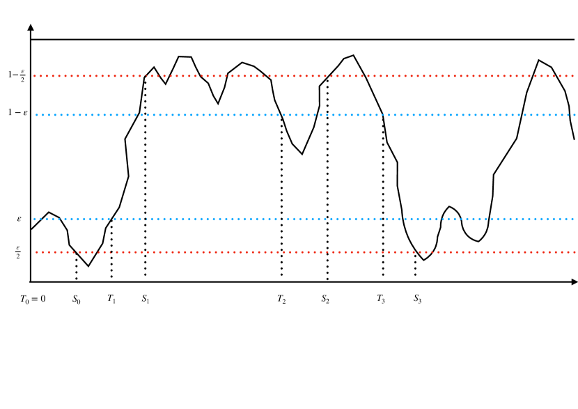
Figure 5.1. Decomposition of trajectory.

Let us start with a useful lemma, which shows that the damping does not need to be controlled outside the excursion intervals $\bigsqcup_{j}[T_{j},S_{j}]$.

Lemma 5.1.

Assume $0\leq{\rm d}_{\mathbb{H}}(\pi^{\gamma},{\mathbb{X}})\leq\varepsilon<\eta<\frac{1}{2}$. For all $t\in[0,H]\backslash\bigsqcup_{j}[T_{j},S_{j}]$, we have:

$$\left|\pi_{t}^{\gamma}-{\mathbf{x}}_{t}\right|\leq\varepsilon\ ,$$

on the event $\{M^{*}<1-2\eta\}\cap\Omega_{\eta}$.

Proof.

By definition, we have for such times $t$:

$$\pi_{t}^{\gamma}\wedge(1-\pi_{t}^{\gamma})\leq\varepsilon\ ,$$

so that the natural estimator $\hat{{\mathbf{x}}}_{t}:=\mathds{1}_{\{\pi_{t}^{\gamma}>\frac{1}{2}\}}$ is easily determined.

By definition of Hausdorff, there exists a pair $(s,x)\in[0,H]\times{\mathbb{X}}_{s}$ such that

$$|t-s|^{2}+|x-\pi_{t}^{\gamma}|^{2}\leq{\rm d}_{\mathbb{H}}(\pi^{\gamma},{\mathbb{X}})^{2}\ ,$$

which implies

$$|x-\hat{{\mathbf{x}}}_{t}|\leq|x-\pi_{t}^{\gamma}|+|\pi_{t}^{\gamma}-\hat{{\mathbf{x}}}_{t}|\leq{\rm d}_{\mathbb{H}}(\pi^{\gamma},{\mathbb{X}})+\varepsilon\leq 2\varepsilon\ .$$

On the event $\{M^{*}<1-2\eta\}$, it entails that

$$|x-{\mathbf{x}}_{s}|\leq M^{*}<1-2\eta\ .$$

Necessarily

$$|{\mathbf{x}}_{s}-\hat{{\mathbf{x}}}_{t}|<1-2\eta+2\varepsilon<1\ ,$$

which amounts to equality. Using that $|s-t|\leq\varepsilon<\eta$, there are no jumps between $s$ and $t$ on the event $\Omega_{\eta}$. We thus have ${\mathbf{x}}_{s}={\mathbf{x}}_{t}=\hat{{\mathbf{x}}}_{t}$. ∎

We consider the event ${\tilde{\Omega}}_{\eta}$ such that for $\mathbb{X}$ all the spikes have size between $\eta$ and $1-\eta$ and the inter-distance between successive spikes/jumps is at least $2\eta$. By definition of $\mathbb{X}$ we have that

$$\lim_{\eta\to 0}\mathbb{P}({\tilde{\Omega}}_{\eta})=1\ .$$

For any $\varepsilon<\eta$ let us consider

$$I=I_{\varepsilon}^{\gamma}:=\left\{j\in\{1,\ldots,N^{\varepsilon}_{\gamma}\}\;;\;[T_{j},S_{j}]\cap K_{\varepsilon}\neq\emptyset\right\}\ .$$ (5.3)

Separation argument: A single segment $[T_{j},S_{j}]$ corresponds, in the large $\gamma$ limit, to either a spike of size larger than $\varepsilon$, or a jump. Because $[T_{j},S_{j}]\cap K_{\varepsilon}\neq\emptyset$, we are far from jumps and the segment $[T_{j},S_{j}]$ necessarily corresponds to a spike. Notice that multiple $[T_{j},S_{j}]$ can correspond to the same spike – see Fig. 5.2. However, a single spike $\{s\}\times{\mathbb{X}}_{s}$ of size larger than $\varepsilon$ in the limiting process determines multiple $[T_{j},S_{j}]$. For a spike $\{s\}\times\mathbb{X}_{s}$, with $0\leq s\leq H$, we denote them by $I_{\varepsilon}(s)$ the finite set:

$$I_{\varepsilon}(s):=\left\{j\in{\mathbb{N}}\ |\ [T_{j},S_{j}]=[T_{j}^{\gamma},S_{j}^{\gamma}]\textrm{ asymptotically coalesces to the spike }\{s\}\times{\mathbb{X}}_{s}\right\}\ .$$

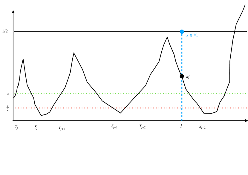
Figure 5.2. Microscopic spike.

Now because of the Hausdorff convergence of $\pi^{\gamma}$ to ${\mathbb{X}}$ and the fact that spikes larger than $\varepsilon$ are separated by a random constant $S_{\varepsilon}>0$, we have that:

$$s\neq s^{\prime}\implies{\rm d}(\cup_{j\in I_{\varepsilon}(s)}[T_{j},S_{j}],\cup_{j\in I_{\varepsilon(s^{\prime})}}[T_{j},S_{j}])>S_{\varepsilon}-{\rm d}_{\mathbb{H}}({\mathcal{G}}(\pi^{\gamma}),\mathbb{X})\ .$$

Thanks to this, supposing the spike at $s$ is starting from $0$, i.e. $\pi_{T_{j}}^{\gamma}=\varepsilon$, we can strengthen the claim:

$$\forall u\in[T_{j},S_{j}],\quad 1-\tfrac{\varepsilon}{2}\geq\pi^{\gamma}_{u}$$

for any $j\in I_{s}$ to

$$\forall u\in\left[T_{j},S_{j}\vee\left(T_{j}+S_{\varepsilon}-{\rm d}_{\mathbb{H}}({\mathcal{G}}(\pi^{\gamma}),\mathbb{X})\right)\right],\quad 1-\tfrac{\varepsilon}{2}\geq\pi^{\gamma}_{u}\ .$$ (5.4)

Proposition 5.2.

Recall the definition of the damping term $D^{\gamma}$ given in Eq. (3.5) and of the set $I_{\varepsilon}^{\gamma}$ in Eq. (5.3). Assume that either

$$C<2\quad\textrm{ and }\quad\forall\varepsilon>0,\quad\lim_{\gamma\rightarrow\infty}\;\sup_{j\in I_{\varepsilon}^{\gamma}}\sup_{t\in[T_{j},S_{j}]}D_{t}^{\gamma}=0\$$ (5.5)

or

$$C>2\quad\textrm{ and }\quad\forall\varepsilon>0,\quad\lim_{\gamma\rightarrow\infty}\inf_{j\in I_{\varepsilon}^{\gamma}}\inf_{t\in[T_{j},S_{j}]}D_{t}^{\gamma}=\infty\ .$$ (5.6)

Then we have

$$\lim_{\gamma\to\infty}{\rm d}_{\mathbb{H}}(\mathcal{G}^{\gamma},\mathcal{G}^{\infty})=0$$

Proof.

By Proposition 4.1 and triangular inequality it is sufficient to prove

$$\lim_{\gamma\to\infty}{\rm d}_{\mathbb{H}}(\mathcal{G}^{\gamma,\circ},\mathcal{G}^{\infty})=0\ .$$

Case 1: $C<2$. Then $\mathcal{G}^{\infty}=\mathbb{X}$ and thanks to the triangular inequality:

$${\rm d}_{\mathbb{H}}(\mathcal{G}^{\gamma,\circ},\mathbb{X})\leq{\rm d}_{\mathbb{H}}(\mathcal{G}^{\gamma,\circ},\mathcal{G}\left(\pi^{\gamma}\right))+{\rm d}_{\mathbb{H}}(\mathcal{G}\left(\pi^{\gamma}\right),{\mathbb{X}})\ .$$

The second term goes to zero thanks to Theorem 2.2 of [BCC⁺22]. It thus suffices to show that

$$\lim_{\gamma\to\infty}{\rm d}_{\mathbb{H}}(\mathcal{G}^{\gamma,\circ},\mathcal{G}\left(\pi^{\gamma}\right))=0\ .$$ (5.7)

As such, starting with the definition of Hausdorff distance:

$$\begin{split}{\rm d}_{\mathbb{H}}(\mathcal{G}^{\gamma,\circ},\mathcal{G}\left(\pi^{\gamma}\right))&=\sup_{\begin{subarray}{c}a\in{\mathcal{G}}^{\gamma,\circ}\\ b\in{\mathcal{G}}(\pi^{\gamma})\end{subarray}}\left\{{\rm d}\left(a,{\mathcal{G}}(\pi^{\gamma})\right),{\rm d}\left(b,\mathcal{G}^{\gamma,\circ}\right)\right\}\\ &\leq\sup_{a\in{\mathcal{G}}^{\gamma,\circ}}{\rm d}\left(a,{\mathcal{G}}(\pi^{\gamma})\right)+\sup_{b\in{\mathcal{G}}(\pi^{\gamma})}{\rm d}\left(b,\mathcal{G}^{\gamma,\circ}\right)\\ &\leq\sup_{a\in{\mathcal{G}}^{\gamma,\circ}\cap K_{\varepsilon}^{\square}}{\rm d}\left(a,{\mathcal{G}}(\pi^{\gamma})\right)+\sup_{a\in{\mathcal{G}}^{\gamma,\circ}\cap J_{\varepsilon}^{\square}}{\rm d}\left(a,{\mathcal{G}}(\pi^{\gamma})\right)\\ &+\sup_{b\in{\mathcal{G}}(\pi^{\gamma})\cap K_{\varepsilon}^{\square}}{\rm d}\left(b,\mathcal{G}^{\gamma,\circ}\right)+\sup_{b\in{\mathcal{G}}(\pi^{\gamma})\cap J_{\varepsilon}^{\square}}{\rm d}\left(b,\mathcal{G}^{\gamma,\circ}\right)\ .\end{split}$$ (5.8)

On $K_{\varepsilon}^{\square}$, we are dealing with graphs of functions, so that

$$\sup_{a\in{\mathcal{G}}^{\gamma,\circ}}{\rm d}\left(a,{\mathcal{G}}(\pi^{\gamma})\right) =\sup_{t\in K_{\varepsilon}}{\rm d}\left({\mathbf{x}}_{t}+(\pi_{t}^{\gamma}-{\mathbf{x}}_{t})e^{-D_{t}^{\gamma}},{\mathcal{G}}(\pi^{\gamma})\right)$$

$$\leq\sup_{t\in K_{\varepsilon}}\left|{\mathbf{x}}_{t}+\left(\pi_{t}^{\gamma}-{\mathbf{x}}_{t}\right)e^{-D_{t}^{\gamma}}-\pi^{\gamma}_{t}\right|$$

where the inequality comes from a ‘slice by slice’ bound. The same argument gives that

$$\sup_{b\in{\mathcal{G}}(\pi^{\gamma})\cap K_{\varepsilon}^{\square}}{\rm d}\left(b,\mathcal{G}^{\gamma,\circ}\right)\leq\sup_{t\in K_{\varepsilon}}\left|{\mathbf{x}}_{t}+\left(\pi_{t}^{\gamma}-{\mathbf{x}}_{t}\right)e^{-D_{t}^{\gamma}}-\pi^{\gamma}_{t}\right|\ .$$

Recalling Eq. (5.8), we get

$$\begin{split}{\rm d}_{\mathbb{H}}(\mathcal{G}^{\gamma,\circ},\mathcal{G}\left(\pi^{\gamma}\right))&\leq 2\sup_{t\in K_{\varepsilon}}\left|{\mathbf{x}}_{t}+\left(\pi_{t}^{\gamma}-{\mathbf{x}}_{t}\right)e^{-D_{t}^{\gamma}}-\pi^{\gamma}_{t}\right|\\ &+\sup_{a\in{\mathcal{G}}^{\gamma,\circ}\cap J_{\varepsilon}^{\square}}{\rm d}\left(a,{\mathcal{G}}(\pi^{\gamma})\right)+\sup_{b\in{\mathcal{G}}(\pi^{\gamma})\cap J_{\varepsilon}^{\square}}{\rm d}\left(b,\mathcal{G}^{\gamma,\circ}\right)\\ &\leq 2\sup_{t\in K_{\varepsilon}}\left|\pi_{t}^{\gamma}-{\mathbf{x}}_{t}\right|\left(1-e^{-D_{t}^{\gamma}}\right)\\ &+\sup_{a\in{\mathcal{G}}^{\gamma,\circ}\cap J_{\varepsilon}^{\square}}{\rm d}\left(a,{\mathcal{G}}(\pi^{\gamma})\right)+\sup_{b\in{\mathcal{G}}(\pi^{\gamma})\cap J_{\varepsilon}^{\square}}{\rm d}\left(b,\mathcal{G}^{\gamma,\circ}\right)\\ &\leq 2\sup_{t\in K_{\varepsilon}}\left|\pi_{t}^{\gamma}-{\mathbf{x}}_{t}\right|\left(1-e^{-D_{t}^{\gamma}}\right)\\ &+\sup_{a\in J_{\varepsilon}^{\square}}{\rm d}\left(a,{\mathcal{G}}(\pi^{\gamma})\right)+\sup_{b\in J_{\varepsilon}^{\square}}{\rm d}\left(b,\mathcal{G}^{\gamma,\circ}\right)\ .\end{split}$$

Now, any point in $J_{\varepsilon}^{\square}$ is at most at distance $\varepsilon$ of $J_{0}^{\square}=\sqcup_{i}\{J_{i}\}\times[0,1]$. This gives:

$$\begin{split}{\rm d}_{\mathbb{H}}(\mathcal{G}^{\gamma,\circ},\mathcal{G}\left(\pi^{\gamma}\right))&\leq 2\varepsilon+\sup_{a\in J_{0}^{\square}}{\rm d}\left(a,{\mathcal{G}}(\pi^{\gamma})\right)+\sup_{b\in J_{0}^{\square}}{\rm d}\left(b,\mathcal{G}^{\gamma,\circ}\right)\\ &+2\sup_{t\in K_{\varepsilon}}\left|\pi_{t}^{\gamma}-{\mathbf{x}}_{t}\right|\left(1-e^{-D_{t}^{\gamma}}\right)\ .\end{split}$$

Because $\mathcal{G}^{\gamma,\circ}$ contains the set of vertical lines $J_{0}^{\square}$, $\sup_{b\in J_{0}^{\square}}{\rm d}\left(b,\mathcal{G}^{\gamma,\circ}\right)=0$. Regarding the term $\sup_{a\in J_{0}^{\square}}{\rm d}\left(a,{\mathcal{G}}(\pi^{\gamma})\right)$, we know that

$$\forall 1\leq j\leq N,\quad\exists s,s^{\prime}\in[J_{j}-\varepsilon,J_{j}+\varepsilon]\text{\rm{ s.t. }}\pi_{s}^{\gamma}\leq\eta_{\gamma},\quad 1-\pi_{s^{\prime}}^{\gamma}\leq\eta_{\gamma}$$ (5.9)

with $\lim_{\gamma\to\infty}\eta_{\gamma}=0$. This claim can be proved exactly as for Eq. (4.22), replacing $\pi^{\delta_{\gamma},\gamma}$ by the simpler process $\pi^{\gamma}$ during the proof. Since $\pi^{\gamma}$ has continuous trajectories, the Intermediate Value Theorem implies that

$$\lim_{\gamma\to\infty}\sup_{a\in J_{0}^{\square}}{\rm d}\left(a,{\mathcal{G}}(\pi^{\gamma})\right)=0\ .$$

Therefore, by sending $\varepsilon$ to $0$ after sending $\gamma$ to infinity, Eq. (5.7) is proved once we show that

$$\begin{split}\limsup_{\varepsilon\to 0}\limsup_{\gamma\to\infty}\sup_{t\in K_{\varepsilon}}\left|\pi_{t}^{\gamma}-{\mathbf{x}}_{t}\right|\left(1-e^{-D_{t}^{\gamma}}\right)=0\ .\end{split}$$ (5.10)

Observe now that

$$\sup_{t\in K_{\varepsilon}}\left|\pi_{t}^{\gamma}-{\mathbf{x}}_{t}\right|\left(1-e^{-D_{t}^{\gamma}}\right)$$

$$\leq \sup_{j\leq N}\left\{\sup_{t\in K_{\varepsilon}\cap[T_{j},S_{j}]}\left|\pi_{t}^{\gamma}-{\mathbf{x}}_{t}\right|\left(1-e^{-D_{t}^{\gamma}}\right)+\sup_{t\notin\sqcup[T_{j},S_{j}]}\left|\pi_{t}^{\gamma}-{\mathbf{x}}_{t}\right|\right\}$$

$$\leq \sup_{j\in I_{\varepsilon}^{\gamma}}\left\{\sup_{t\in K_{\varepsilon}\cap[T_{j},S_{j}]}\left(1-e^{-D_{t}^{\gamma}}\right)+\sup_{t\notin\sqcup[T_{j},S_{j}]}\left|\pi_{t}^{\gamma}-{\mathbf{x}}_{t}\right|\right\}\ .$$

Thanks to Lemma 5.1, we find on the good event, that

$$\limsup_{\varepsilon\to 0}\limsup_{\gamma\to\infty}\left\{\sup_{t\in K_{\varepsilon}}\left|\pi_{t}^{\gamma}-{\mathbf{x}}_{t}\right|\left(1-e^{-D_{t}^{\gamma}}\right)\right\}$$

$$\leq \limsup_{\varepsilon\to 0}\limsup_{\gamma\to\infty}\left\{\sup_{j\in I_{\varepsilon}^{\gamma}}\;\sup_{t\in K_{\varepsilon}\cap[T_{j},S_{j}]}\left(1-e^{-D_{t}^{\gamma}}\right)\right\}\ .$$

In the last line we used also Eq. (5.3). Because of the inequality $1-e^{-x}\leq x$ for all $x\geq 0$, Eq. (5.10) follows from assumption (5.5) and the proof is complete.

Case 2: $C>2$. Here ${\mathcal{G}}^{\infty}={\mathcal{G}}({\mathbf{x}})$. The proof in this case is slightly different. By Eq. (4.8), we have that

$${\rm d}_{\mathbb{H}}({\mathcal{G}}^{\gamma,\circ},{\mathcal{G}}({\mathbf{x}})) \leq{\rm d}_{\mathbb{H}}\left({\mathcal{G}}^{\gamma,\circ}\cap J_{\varepsilon}^{\square},{\mathcal{G}}({\mathbf{x}})\cap J_{\varepsilon}^{\square}\right)+{\rm d}_{\mathbb{H}}\left({\mathcal{G}}^{\gamma,\circ}\cap K_{\varepsilon}^{\square},{\mathcal{G}}({\mathbf{x}})\cap K_{\varepsilon}^{\square}\right)\ .$$

Since the graphs ${\mathcal{G}}({\mathbf{x}})$ and ${\mathcal{G}}^{\gamma,\circ}$ contain both the set $J_{0}^{\square}$ of vertical lines, we get easily that

$$\limsup_{\varepsilon\to 0}\limsup_{\gamma\to\infty}{\rm d}_{\mathbb{H}}\left({\mathcal{G}}^{\gamma,\circ}\cap J_{\varepsilon}^{\square},J_{\varepsilon}^{\square}\right)=0$$

and

$$\limsup_{\varepsilon\to 0}{\rm d}_{\mathbb{H}}\left({\mathcal{G}}({\mathbf{x}})\cap J_{\varepsilon}^{\square},J_{\varepsilon}^{\square}\right)=0$$

so that it remains only to prove that

$$\limsup_{\varepsilon\to 0}\limsup_{\gamma\to\infty}{\rm d}_{\mathbb{H}}\left({\mathcal{G}}^{\gamma,\circ}\cap K_{\varepsilon}^{\square},{\mathcal{G}}({\mathbf{x}})\cap K_{\varepsilon}^{\square}\right)=0\ .$$

Since, on $K_{\varepsilon}$, we are dealing with the graphs of functions, we give a bound ‘slice by slice’:

$${\rm d}_{\mathbb{H}}\left({\mathcal{G}}^{\gamma,\circ}\cap K_{\varepsilon}^{\square},{\mathcal{G}}({\mathbf{x}})\cap K_{\varepsilon}^{\square}\right)$$

$$\leq \sup_{t\in K_{\varepsilon}}\left|{\mathbf{x}}_{t}+\left(\pi_{t}^{\gamma}-{\mathbf{x}}_{t}\right)e^{-D_{t}^{\gamma}}-{\mathbf{x}}_{t}\right|$$

$$\leq \sup_{t\in K_{\varepsilon}}\left|\pi_{t}^{\gamma}-{\mathbf{x}}_{t}\right|e^{-D_{t}^{\gamma}}$$

$$\leq \sup_{j\leq N}\sup_{t\in K_{\varepsilon}\cap[T_{j},S_{j}]}e^{-D_{t}^{\gamma}}+\sup_{t\notin\sqcup[T_{j},S_{j}]}\left|\pi_{t}^{\gamma}-{\mathbf{x}}_{t}\right|$$

$$\leq \exp\left(-\inf_{j\leq N}\inf_{t\in K_{\varepsilon}\cap[T_{j},S_{j}]}D_{t}^{\gamma}\right)+\sup_{t\notin\sqcup[T_{j},S_{j}]}\left|\pi_{t}^{\gamma}-{\mathbf{x}}_{t}\right|\ .$$

Thanks to Lemma 5.1, we find on the good event:

$${\rm d}_{\mathbb{H}}\left({\mathcal{G}}^{\gamma,\circ}\cap K_{\varepsilon}^{\square},{\mathcal{G}}(\pi^{\gamma})\cap K_{\varepsilon}^{\square}\right)$$

$$\leq \varepsilon+\exp\left(-\inf_{j\leq N}\inf_{t\in K_{\varepsilon}\cap[T_{j},S_{j}]}D_{t}^{\gamma}\right)$$

$$= \varepsilon+\exp\left(-\inf_{j\in I_{\varepsilon}^{\gamma}}\inf_{t\in K_{\varepsilon}\cap[T_{j},S_{j}]}D_{t}^{\gamma}\right)\ .$$

Notice in the last equality the appearance of the index set $I_{\varepsilon}^{\gamma}$ because if $j\notin I_{\varepsilon}^{\gamma}$ then $K_{\varepsilon}\cap[T_{j},S_{j}]=\emptyset$ (see the definition in Eq. (5.3)). This latter bound goes to zero by assumption (5.6). ∎

5.2. Coordinates via logistic regression

In the previous paper [BCC⁺22], a crucial role was played by the scale function which is the unique change of variable $f=h_{\gamma}$ such that $f(\pi_{t}^{\gamma})$ is a martingale. This uniqueness is of course up to affine transformations. Another useful change of variable is as follows. Instead of asking for a vanishing drift, one can ask for a constant volatility term.

Lemma 5.3.

Recall Eq. (2.4). Up to affine transformations, the unique function $f:(0,1)\to\mathbb{R}$ such that $f(\pi^{\gamma})$ has constant volatility term is the logistic function

$$f:x\in(0,1)\to f(x):=\log\frac{x}{1-x}\ .$$

The process $Y_{t}^{\gamma}:=f(\pi_{t}^{\gamma})$ satisfies:

$$dY_{t}^{\gamma}= \sqrt{\gamma}dW_{t}+\left(\lambda(2p-1)+\lambda pe^{-Y_{t}}-\lambda(1-p)e^{Y_{t}}+\dfrac{\gamma}{2}\tanh\left(\tfrac{Y_{t}}{2}\right)\right)dt$$ (5.11)

$$= \sqrt{\gamma}dB_{t}+\left(\lambda(2p-1)+\lambda pe^{-Y_{t}}-\lambda(1-p)e^{Y_{t}}+\gamma\left({\mathbf{x}}_{t}-\frac{1}{2}\right)\right)dt\$$ (5.12)

where $(W_{t}\;;\;t\geq 0)$ and $(B_{t}\;;\;t\geq 0)$ are related by Eq. (2.5).

Proof.

In order to lighten notation we omit the superscript $\gamma$ in the next equations. For a given smooth function $f$, Itô formula yields

$$df(\pi_{t})= \left(-f^{\prime}(\pi_{t})\lambda(\pi_{t}-p)+\frac{1}{2}\gamma f^{\prime\prime}(\pi_{t})\pi_{t}^{2}(1-\pi_{t})^{2}\right)dt+f^{\prime}(\pi_{t})\pi_{t}(1-\pi_{t})\sqrt{\gamma}dW_{t}\ .$$

As such, $f(\pi_{t})$ has constant volatility term, say $\sqrt{\gamma}$, if and only if:

$$1=f^{\prime}(x)x(1-x)\Longleftrightarrow\ f(x)=\log\frac{x}{1-x}+\log\kappa\ ,$$

for a certain choice of constant $\kappa>0$. The first claim is proved.

Now, choosing $\kappa=1$ for convenience, let us derive the SDE for $Y=f(\pi)$. By using $f^{\prime}(x)=\tfrac{1}{x(1-x)},\quad f^{\prime\prime}(x)=\tfrac{2x-1}{x^{2}(1-x)^{2}}\ ,$ we obtain:

$$dY_{t}= \left(-\lambda\frac{\pi_{t}-p}{\pi_{t}(1-\pi_{t})}+\frac{1}{2}\gamma\left(2\pi_{t}-1\right)\right)dt+\sqrt{\gamma}dW_{t}$$

$$= \left(\lambda p+\lambda pe^{-Y_{t}}-\lambda(1-p)e^{Y_{t}}-\lambda(1-p)+\frac{1}{2}\gamma\left(2\pi_{t}-1\right)\right)dt+\sqrt{\gamma}dW_{t}\ \ ,$$

hence the first expression (5.11) with $2\pi_{t}-1=\frac{2}{1+e^{-Y_{t}}}-1=\tanh(\tfrac{Y_{t}}{2})$.

For the second expression (5.12), recalling that $dW_{t}=dB_{t}+\sqrt{\gamma}\left({\mathbf{x}}_{t}-\pi_{t}\right)dt\ ,$ we get:

$$dY_{t}= \left(\lambda(2p-1)+\lambda pe^{-Y_{t}}-\lambda(1-p)e^{Y_{t}}+\frac{1}{2}\gamma\left(2\pi_{t}-1\right)+\gamma\left({\mathbf{x}}_{t}-\pi_{t}\right)\right)dt+\sqrt{\gamma}dB_{t}$$

$$= \left(\lambda(2p-1)+\lambda pe^{-Y_{t}}-\lambda(1-p)e^{Y_{t}}+\gamma\left({\mathbf{x}}_{t}-\frac{1}{2}\right)\right)dt+\sqrt{\gamma}dB_{t}\ .$$

∎

Given this information the instantaneous damping term in Eq. (3.2) takes a particularly convenient expression:

$$a_{t}^{\gamma}= \lambda pe^{Y_{t}^{\gamma}}+\lambda(1-p)e^{-Y_{t}^{\gamma}}\ .$$ (5.13)

Discussion:

In particular, in order to prove that the damping term $D^{\gamma}$ in Eq. (3.5) either converges to zero or diverges to infinity, it suffices to control for $|t-s|\ll 1$:

$$D^{\gamma}_{t}=\int_{t-\delta_{\gamma}}^{t}a_{u}^{\gamma}du\asymp\int_{t-\delta_{\gamma}}^{t}\left(e^{Y^{\gamma}_{u}}+e^{-Y^{\gamma}_{u}}\right)du\ .$$

Depending on whether $\pi^{\gamma}_{u}\approx 0$ ($Y^{\gamma}_{u}\approx-\infty$) or $\pi^{\gamma}_{u}\approx 1$ ($Y^{\gamma}_{u}\approx\infty$), one of the two expressions is dominant. Assuming $\pi^{\gamma}_{u}\approx 0$ on the entire interval $[t-\delta_{\gamma},t]$, we have:

$$\int_{t-\delta_{\gamma}}^{t}a_{u}^{\gamma}du\asymp\int_{t-\delta_{\gamma}}^{t}e^{-Y^{\gamma}_{u}}du\ .$$

Continuing:

$$Y_{u}-Y_{s}= \sqrt{\gamma}\left(W_{u}-W_{s}\right)+\int_{s}^{u}\left(\frac{\lambda p}{\pi_{v}}-\frac{\lambda(1-p)}{1-\pi_{v}}+\frac{1}{2}\gamma\left(2\pi_{v}-1\right)\right)du$$

$$= \sqrt{\gamma}\left(W_{u}-W_{s}\right)-\frac{1}{2}\gamma(u-s)+\int_{s}^{u}\left(\frac{\lambda p}{\pi_{v}}-\frac{\lambda(1-p)}{1-\pi_{v}}+\gamma\pi_{v}\right)dv\ .$$

We have thus proved the expression which is useful for $\pi_{u}\approx 0$:

$$Y_{u}-Y_{s}= \sqrt{\gamma}\left(W_{u}-W_{s}\right)-\frac{1}{2}\gamma(u-s)+\int_{s}^{u}\left(\frac{\lambda p}{\pi_{v}}-\frac{\lambda(1-p)}{1-\pi_{v}}+\gamma\pi_{v}\right)dv\ .$$ (5.14)

If $\pi_{u}\approx 1$, then the useful expression is:

$$Y_{u}-Y_{s}= \sqrt{\gamma}\left(W_{u}-W_{s}\right)+\frac{1}{2}\gamma(u-s)+\int_{s}^{u}\left(\frac{\lambda p}{\pi_{v}}-\frac{\lambda(1-p)}{1-\pi_{v}}-\gamma(1-\pi_{v})\right)dv\ .$$ (5.15)

Path transforms: In order to systematically control the fluctuations of the process $Y$, we make the following change of variables. For $t\geq 0$, define:

$$a_{t}:= \ Y_{t}-\log\left(\lambda p\right)\ ,$$ (5.16)

$$b_{t}:= \ \sqrt{\gamma}W_{t}-\frac{\gamma}{2}t+r_{t}\ ,$$ (5.17)

$$r_{t}:= \ \int_{0}^{t}du\left(\lambda(2p-1)-\lambda(1-p)e^{Y_{u}}+\frac{\gamma}{2}\left(1+\tanh(\frac{Y_{u}}{2})\right)\right)\ .$$ (5.18)

The choice of letter for $r$ is that it will later play the role of residual quantity. Thanks to this reformulation, the SDE defining $Y$ in Eq. (5.11) becomes:

$$da_{t}= \ db_{t}+e^{-a_{t}}dt\ .$$ (5.19)

The following lemma gives two ways of integrating Eq. (5.19) – in the sense that we consider $b$ known and $a$ unknown.

Lemma 5.4.

Consider two real-valued semi-martingales $a$ and $b$ satisfying Eq. (5.19). Then for all $0\leq s\leq t$, we have the backward and forward formulas:

$$a_{s,t}=b_{s,t}-\log\left(1-\frac{1}{e^{a_{t}}}\int_{s}^{t}e^{b_{u,t}}du\right)\ .$$

$$a_{s,t}=b_{s,t}+\log\left(1+\frac{1}{e^{a_{s}}}\int_{s}^{t}e^{-b_{s,u}}du\right)\ .$$

Proof.

We start by writing:

$$a_{s,t}=b_{s,t}+\int_{s}^{t}e^{-a_{u}}du\ .$$

Backward integration: Consider $t$ as fixed and $s$ as vaying. Then differentiate in $s$ the expression for $s\leq t$:

$$a_{s,t}=b_{s,t}+\frac{1}{e^{a_{t}}}\int_{s}^{t}e^{a_{u,t}}du\ .$$

It yields:

$$\frac{d}{ds}\left(a_{s,t}-b_{s,t}\right)=-\frac{1}{e^{a_{t}}}e^{a_{s,t}}=-\frac{1}{e^{a_{t}}}e^{a_{s,t}-b_{s,t}}e^{b_{s,t}}\ .$$

Equivalently:

$$\frac{d}{ds}\left(e^{-(a_{s,t}-b_{s,t})}\right)=\frac{1}{e^{a_{t}}}e^{b_{s,t}}\ .$$

Integrating between on $[s,t]$ gives:

$$1-e^{-(a_{s,t}-b_{s,t})}=\frac{1}{e^{a_{t}}}\int_{s}^{t}e^{b_{u,t}}du\ ,$$

which gives the backward formula.

Forward integration: The other way around, fix $s$ and take $t$ as vaying. Then differentiate in $s$ the expression for $s\leq t$:

$$a_{s,t}=b_{s,t}+\frac{1}{e^{a_{s}}}\int_{s}^{t}e^{-a_{s,u}}du\ .$$

It yields:

$$\frac{d}{dt}\left(a_{s,t}-b_{s,t}\right)=\frac{1}{e^{a_{s}}}e^{-a_{s,t}}=\frac{1}{e^{a_{s}}}e^{-(a_{s,t}-b_{s,t})}e^{-b_{s,t}}\ .$$

Equivalently:

$$\frac{d}{dt}\left(e^{a_{s,t}-b_{s,t}}\right)=\frac{1}{e^{a_{s}}}e^{-b_{s,t}}\ .$$

Integrating between on $[s,t]$ gives:

$$e^{a_{s,t}-b_{s,t}}-1=\frac{1}{e^{a_{s}}}\int_{s}^{t}e^{-b_{s,u}}du\ ,$$

which gives the forward formula. ∎

Controlling the residual $r$: Recall that in the context of Proposition 4.1 and the expression of the damping term in Eq. (5.13), we need to control:

$$D_{t}=\int_{s=t-\delta_{\gamma}}^{t}a_{u}du\ .$$

As such the relevant time inequalities are $T_{j}-\delta_{\gamma}\leq s\leq u\leq t\leq S_{j}$.

Let $(s_{k})_{k}$ be the sequence of ordered times of the spikes of length greater than $\varepsilon$ in $[0,H]$. For fixed $\varepsilon$ they are in (random) finite number, say $k_{\varepsilon}$. We have

$$I_{\varepsilon}^{\gamma}=\sqcup_{\ell=1}^{k_{\varepsilon}}\ I_{\varepsilon}(s_{\ell})\cap I_{\varepsilon}^{\gamma}$$

and, thanks to the separation argument and the fact that $\sum_{i}|S_{i}-T_{i}|=\mathcal{O}_{\varepsilon}(1/\gamma)$, there exists a constant $C(\varepsilon)$ such that for any $i\in I_{\varepsilon}(s_{\ell})\cap I_{\varepsilon}^{\gamma}$ and any $v\in[T_{i},S_{i}]$, $|v-s_{\ell}|\leq C(\varepsilon)/\gamma$.

Let us denote by $j\in I_{\varepsilon}^{\gamma}$ the integer such that $t\in[T_{j},S_{j}]$ and by $k\in\{1,\ldots,k_{\varepsilon}\}$ the integer such that $j\in I_{\varepsilon}(s_{k})$. To simplify notation we write $s=t-\delta_{\gamma}$. We have that

$$|s-s_{k}|\leq\delta_{\gamma}+C(\varepsilon)/\gamma\ .$$ (5.20)

Examining this specific interval $[S_{j},T_{j}]$, it corresponds to one of the following two situations

1. $\pi_{T_{j}}^{\gamma}=1-\varepsilon,\,\pi_{S_{j}}^{\gamma}=1-\varepsilon/2$: in the limit, it is a spike from $1$ to $1$ for $\mathbb{X}$ ;

2. $\pi_{T_{j}}^{\gamma}=\varepsilon,\,\pi_{S_{j}}^{\gamma}=\varepsilon/2$: in the limit, it is a spike from $0$ to $0$ for $\mathbb{X}$ .

By symmetry, we only have to consider case ii).

Lemma 5.5.

For all indices $j$ such that correspond to a spike from $0$ to $0$, we have

$$\sup_{T_{j}-\delta_{\gamma}\leq s\leq t\leq S_{j}}|r_{s,t}|=o_{\varepsilon}(\log\gamma)\ .$$ (5.21)

The implied constant is random yet finite, depends on $\varepsilon>0$ but is independent of $j$ and $\gamma$.

Proof.

By definition of the $T_{i}$’s and $S_{i}$’s, we have that $1-\varepsilon/2\geq\pi_{u}^{\gamma}\geq\varepsilon/2$ for $u\in[T_{j},S_{j}]$. In fact, thanks to the separation argument, the left bound holds on a much longer interval just like in Eq. (5.4). As such, for $S_{\varepsilon}-{\rm d}_{\mathbb{H}}({\mathcal{G}}(\pi^{\gamma}),\mathbb{X})>\delta_{\gamma}$, we have

$$\sup_{T_{j}-\delta_{\gamma}\leq u\leq S_{j}}\pi_{u}\leq 1-\varepsilon/2$$ (5.22)

which implies

$$\sup_{T_{j}-\delta_{\gamma}\leq u\leq S_{j}}Y_{u}^{\gamma}\leq{\mathcal{O}}_{\varepsilon}(1)\ .$$

Again within the range $T_{j}-\delta_{\gamma}\leq s\leq u\leq t\leq S_{j}$, let us control the process $r$ from Eq. (5.18). We have:

$$\left|r_{s,t}\right|\leq \ \left[\lambda(2p-1)+\lambda(1-p)\exp(\sup_{T_{j}-\delta_{\gamma}\leq u\leq S_{j}}Y_{u}^{\gamma})\right](t-s)+\frac{\gamma}{2}\int_{s}^{t}\left(1+\tanh(\frac{Y_{u}}{2})\right)du$$

$$\leq \ {\mathcal{O}}_{\varepsilon}(1)\left(\delta_{\gamma}+S_{j}-T_{j}\right)+\frac{\gamma}{2}\int_{s}^{t}\pi_{u}du\ ,$$

where we used in the last line the fact that

$$1+\tanh(\frac{Y_{u}}{2})=1+\frac{e^{Y_{u}}-1}{e^{Y_{u}}+1}=\frac{2}{1+e^{-Y_{u}}}=\pi_{u}\ .$$

By Corollary 2.4 in [BCC⁺22] we know that the time spent by $\pi^{\gamma}$ in the interval $[\eta,1-\eta]$ during the time window $[0,H]$ is of order ${\mathcal{O}}_{\eta}(1/\gamma)$. Hence $\sum_{j}|S_{j}-T_{j}|={\mathcal{O}}_{\varepsilon}(1/\gamma)$ and:

$$\left|r_{s,t}\right|\leq \ \ {\mathcal{O}}_{\varepsilon}(1)\left(\delta_{\gamma}+\frac{1}{\gamma}\right)+{\mathcal{O}}_{\eta}(1)+\frac{\gamma}{2}\int_{s}^{t}\pi_{u}\mathds{1}_{\{\pi_{u}<\eta\}}du$$

$$\leq \ {\mathcal{O}}_{\varepsilon}(1)\delta_{\gamma}+{\mathcal{O}}_{\eta}(1)+\frac{\eta\gamma}{2}\left(t-s\right)$$

$$\leq \ {\mathcal{O}}_{\varepsilon}(1)\delta_{\gamma}+{\mathcal{O}}_{\eta}(1)+\eta\gamma{\mathcal{O}}_{\varepsilon}(1)\left(\delta_{\gamma}+\frac{1}{\gamma}\right)\ .$$

Taking $\eta=\eta_{\gamma}\rightarrow 0$ slowly enough so that the second term remains dominated by the third, we have:

$$\left|r_{s,t}\right|\leq \ \ {\mathcal{O}}_{\varepsilon}(\delta_{\gamma})+{\mathcal{O}}_{\varepsilon}(\eta_{\gamma}\log\gamma)$$

$$= \ o_{\varepsilon}(\log\gamma)\ .$$

∎

5.3. Fast feedback regime $C<2$

As announced in Proposition 5.2, we only need to prove an uniform absence of damping:

$$\lim_{\gamma\rightarrow\infty}\sup_{j\in I_{\varepsilon}^{\gamma}}\sup_{t\in[T_{j},S_{j}]}D_{t}^{\gamma}=0\ .$$ (5.23)

We proceed by symmetry as in Lemma 5.5, by considering only spikes from $0$ to $0$. As in the proof of that lemma, we have which implies

$$\sup_{t-\delta_{\gamma}\leq u\leq t}Y_{u}^{\gamma}\leq{\mathcal{O}}_{\varepsilon}(1)\ .$$

Hence:

$$D_{t}^{\gamma}=\int_{s}^{t}a_{u}^{\gamma}du \lesssim\int_{s}^{t}\left(e^{-Y^{\gamma}_{u}}+e^{Y^{\gamma}_{u}}\right)du$$

$$\lesssim\delta_{\gamma}+\int_{s}^{t}e^{-Y^{\gamma}_{u}}du$$

$$=\delta_{\gamma}+e^{-Y^{\gamma}_{t}}\int_{s}^{t}e^{-(Y^{\gamma}_{u}-Y_{t}^{\gamma})}du$$

$$\lesssim\delta_{\gamma}+\int_{s}^{t}e^{Y_{u,t}^{\gamma}}du\ .$$

Let us now control this last term. Thanks to the reformulation of Eq. (5.16–5.18) and then the backward formula of Lemma 5.4 we have:

$$\int_{s}^{t}e^{Y_{u,t}^{\gamma}}du$$

$$= \int_{s}^{t}e^{a_{u,t}^{\gamma}}du$$

$$= \int_{s}^{t}\frac{e^{b_{u,t}^{\gamma}}}{\left(1-\frac{1}{e^{a_{t}}}\int_{u}^{t}e^{b_{v,t}}dv\right)}du$$

$$= e^{a_{t}}\int_{s}^{t}\frac{\frac{1}{e^{a_{t}}}e^{b_{u,t}^{\gamma}}}{\left(1-\frac{1}{e^{a_{t}}}\int_{u}^{t}e^{b_{v,t}}dv\right)}du$$

$$= e^{a_{t}}\int_{s}^{t}d\log\left(1-\frac{1}{e^{a_{t}}}\int_{u}^{t}e^{b_{v,t}}dv\right)$$

$$= -e^{a_{t}}\log\left(1-\frac{1}{e^{a_{t}}}\int_{s}^{t}e^{b_{u,t}}du\right)\ .$$

Going back to the previous equation, we find:

$$D_{t}^{\gamma} \lesssim\delta_{\gamma}-e^{a_{t}}\log\left(1-\frac{1}{e^{a_{t}}}\int_{s}^{t}e^{b_{u,t}}du\right)$$

$$=\delta_{\gamma}-\frac{e^{Y_{t}}}{\lambda p}\log\left(1-\lambda pe^{-Y_{t}}\int_{s}^{t}e^{r_{u,t}+\sqrt{\gamma}W_{u,t}-\frac{\gamma}{2}(t-u)}du\right)\ .$$

Because $t\in[T_{j},S_{j}]$, $\frac{1}{2}\varepsilon\leq Y_{t}\leq\varepsilon$ and therefore it suffices to prove:

$$\sup_{T_{j}-\delta_{\gamma}\leq t\leq S_{j}}\int_{s=t-\delta_{\gamma}}^{t}e^{r_{u,t}+\sqrt{\gamma}W_{u,t}-\frac{\gamma}{2}(t-u)}du\stackrel{{\scriptstyle\gamma\rightarrow\infty}}{{\longrightarrow}}0\ .$$

Now thanks to Lemma 5.5 and Lévy’s modulus of continuity:

$$\int_{s=t-\delta_{\gamma}}^{t}e^{r_{u,t}+\sqrt{\gamma}W_{u,t}-\frac{\gamma}{2}(t-u)}du$$

$$= \int_{0}^{\delta_{\gamma}}e^{r_{t-u,t}+\sqrt{\gamma}W_{t_{u},t}-\frac{\gamma}{2}u}du$$

$$\leq \int_{0}^{\delta_{\gamma}}\exp\left(o_{\varepsilon}(\log\gamma)+\sqrt{\gamma}(1+o(1))\sqrt{2u\log\frac{1}{u}}-\frac{\gamma}{2}u\right)du$$

$$= \frac{2\log\gamma}{\gamma}\int_{0}^{\frac{C}{2}}\gamma^{o_{\varepsilon}(1)}\exp\left((1+o(1))2\sqrt{w\log\gamma\log\frac{\gamma}{2w\log\gamma}}-w\log\gamma\right)dw$$

$$\leq \frac{2\log\gamma}{\gamma}\int_{0}^{\frac{C}{2}}\gamma^{o_{\varepsilon}(1)+(1+o(1))2\sqrt{w}-w}dw$$

$$= 2\log\gamma\int_{0}^{\frac{C}{2}}\gamma^{o_{\varepsilon}(1)-(1-\sqrt{w})^{2}}dw\ .$$

Observe that this upper bound goes to zero as $\gamma\rightarrow\infty$ for any $C<2$. Therefore we are done. We have proved Eq. (5.5), which indeed gives no damping.

Remark 5.6 (On Lévy’s modulus of continuity).

In fact, because of the DDS coupling, $W=W^{\gamma}$ actually depends on $\gamma$. Therefore, the control provided by Lévy’s modulus of continuity is not almost sure. The $o(1)$ has to be understood in the sense of small with high probability.

5.4. Slow feedback regime $C>2$

Here we assume that $C>2$.

We shall prove that there is damping:

$$\lim_{\gamma\rightarrow\infty}\inf_{j}\inf_{t\in[T_{j},S_{j}]}\int_{s=t-\delta_{\gamma}}^{t}a_{u}^{\gamma}du=\infty\ .$$ (5.24)

We know that for $\gamma$ large enough, because $\sum_{j}|S_{j}-T_{j}|={\mathcal{O}}_{\varepsilon}(1/\gamma$, we know that in the above infimum

$$s\leq S_{j}-\delta_{\gamma}<T_{j}\leq t\ .$$

As such, this setting, we need to prove that:

$$\int_{S_{j}-\delta_{\gamma}}^{T_{j}}a_{u}^{\gamma}du\asymp\int_{S_{j}-\delta_{\gamma}}^{T_{j}}\left(e^{Y_{u}}+e^{-Y_{u}}\right)du\rightarrow\infty\ ,$$

for uniformly in $s\in\cup_{j}[T_{j},S_{j}]$ i.e. around spikes. Let us denote by $j$ the integer such that $t\in[T_{j},S_{j}]$. Because there are finitely many $j^{\prime}s$, we need to prove it for a single $j$. Examining this specific interval, if it corresponds to a jump, then it is basically already controlled. Otherwise, it is a spike from $0$ to $0$, or from $1$ to $1$. By symmetry, we assume $\pi_{u}\approx 0$ most of the time. Thus, we only need to prove:

$$\int_{S_{j}-\delta_{\gamma}}^{T_{j}}a_{u}^{\gamma}du\asymp o(1)+\int_{S_{j}-\delta_{\gamma}}^{T_{j}}e^{-Y_{u}}\rightarrow\infty\ .$$

Step 1: Starting backward from $T_{j}$, the process $Y$ reaches $-\log\gamma+K$. Let us prove that there is a $\tau\in[S_{j}-\delta_{\gamma},T_{j}]$ such that:

$$Y_{\tau}=-\log\gamma+K\ ,$$

where $K$ is a large but fixed constant.

Without loss of generality, we can look for $\tau\in[T_{j}-\delta_{\gamma},T_{j}]$. Indeed, by slightly reducing the constant $C>2$ to $2<C^{\prime}<C$, we will have for $\gamma$ large enough $S_{j}-C\frac{\log\gamma}{\gamma}<T_{j}-C^{\prime}\frac{\log\gamma}{\gamma}$.

Now, recall that for $u\leq t\in[T_{j},S_{j}]$:

$$Y_{t}-Y_{t-u}=\sqrt{\gamma}W_{t-u,t}-\frac{1}{2}\gamma u+r_{t-u,t}+\lambda p\int_{t-u}^{t}e^{-Y_{v}}dv\ .$$

If

$$\forall u\leq v\leq t,\ Y_{v}\geq-\log\gamma+K\ ,$$

we have:

$$e^{-K}\lambda p\gamma u-\frac{1}{2}\gamma u+\sqrt{\gamma}W_{t-u,t}+r_{t-u,t}\leq Y_{t-u,t}\leq\log\gamma-K+Y_{t}\leq\log\gamma-K+{\mathcal{O}}_{\varepsilon}(1)\ ,$$

which implies, after using Lemma 5.5:

$$e^{-K}\lambda p\gamma u-\frac{1}{2}\gamma u+\sqrt{\gamma}W_{t-u,t}+o_{\varepsilon}(\log\gamma)\leq\log\gamma-K+{\mathcal{O}}_{\varepsilon}(1)\ .$$

In particular, if $Y$ does not reach $-\log\gamma+K$ on $[t-\delta_{\gamma},t]$, then for all $w\in[0,\frac{1}{2}C]$, we have $u=\frac{2\log\gamma}{\gamma}w\in[0,\delta_{\gamma}]$ and

$$2e^{-K}\lambda pw\log\gamma-w\log\gamma+\sqrt{\gamma}W_{t-u,t}+o_{\varepsilon}(\log\gamma)\leq\log\gamma-K+{\mathcal{O}}_{\varepsilon}(1)\ .$$

Hence

$$\forall t\in[T_{j},S_{j}],\ \forall w\in[0,\frac{1}{2}C],\ \frac{\sqrt{\gamma}}{\log\gamma}W_{t-\frac{2\log\gamma}{\gamma}w,t}\leq o_{\varepsilon}(1)+1+w\left(1-2e^{-K}\lambda p\right)\ .$$

So that:

$$\forall w\in[0,\frac{1}{2}C],\ \frac{\sqrt{\gamma}}{\log\gamma}\sup_{t\in[T_{j},S_{j}]}W_{t-\frac{2\log\gamma}{\gamma}w,t}\leq o_{\varepsilon}(1)+1+w\left(1-2e^{-K}\lambda p\right)\ .$$

Invoking again Lévy’s modulus of continuity on the random interval $[T_{j},S_{j}]$:

$$\forall w\in[0,\frac{1}{2}C],\ (1+o(1))\frac{\sqrt{\gamma}}{\log\gamma}\sqrt{2\frac{2\log\gamma}{\gamma}w\log\frac{\gamma}{2w\log\gamma}}\leq o_{\varepsilon}(1)+1+w\left(1-2e^{-K}\lambda p\right)\ ,$$

which is equivalent to:

$$\forall w\in[0,\frac{1}{2}C],\ (1+o(1))2\sqrt{w}\leq o_{\varepsilon}(1)+1+w\left(1-2e^{-K}\lambda p\right)\ .$$

Taking the limit $\gamma\rightarrow\infty$, gives the clean expression:

$$\forall w\in[0,\frac{1}{2}C],\ 2\sqrt{w}\leq 1+w\left(1-2e^{-K}\lambda p\right)\ .$$

This inequality is clearly violated for $K$ large enough but fixed, and a certain $1<w<\frac{1}{2}C$.

Step 2: Further information.

From the backward formula of Lemma 5.4, we see that:

$$Y_{t-u,t}$$

$$= \sqrt{\gamma}W_{t-u,t}-\frac{\gamma}{2}u-\log\left(1-\lambda pe^{-Y_{t}}\int_{t-u}^{t}e^{r_{v,t}+\sqrt{\gamma}W_{v,t}-\frac{\gamma}{2}(t-v)}dv\right)$$

$$= \sqrt{\gamma}W_{t-u,t}-\frac{\gamma}{2}u-\log\left(1-\lambda pe^{-Y_{t}}\int_{0}^{u}e^{r_{t-v,t}+\sqrt{\gamma}W_{t-v,t}-\frac{\gamma}{2}v}dv\right)\ .$$

Using the modulus of continuity:

$$-Y_{t-u}$$

$$\geq \sqrt{\gamma}W_{t-u,t}-\frac{\gamma}{2}u+o_{\varepsilon}\left(\log\gamma\right)\ .$$

From the forward formula, on the other hand:

$$Y_{t,t+u}$$

$$= \sqrt{\gamma}W_{t,t+u}-\frac{\gamma}{2}u+\log\left(1+\lambda pe^{-Y_{t}}\int_{t}^{t+u}e^{-r_{t,v}-\sqrt{\gamma}W_{t,v}+\frac{\gamma}{2}(v-t)}dv\right)$$

$$= \sqrt{\gamma}W_{t,t+u}-\frac{\gamma}{2}u+\log\left(1+\lambda pe^{-Y_{t}}\int_{0}^{u}e^{-r_{\tau,\tau+v}-\sqrt{\gamma}W_{t,t+v}+\frac{\gamma}{2}v}dv\right)\ ,$$

which easier to control in order to prove a divergence to $\infty$.

As such, we plan on using a forward estimate once we have reached $\tau$. By modifiying the previous step and using the forward formula, we have that $T_{j}-\tau>\frac{c\log\gamma}{\gamma}$ for some small $c>0$.

Step 3: Conclusion. Now, we know that $Y$ reaches $-\log\gamma+K$ at $\tau\in[T_{j}-\delta_{\gamma},T_{j}]$ as soon as $C>2$. Moreover, $\tau-T_{j}$ is sufficiently large.

Because

$$\int_{S_{j}-\delta_{\gamma}}^{T_{j}}a_{u}^{\gamma}du\asymp o(1)+\int_{S_{j}-\delta_{\gamma}}^{T_{j}}e^{-Y_{u}}\geq o(1)+\int_{\tau}^{T_{j}}e^{-Y_{u}}\ ,$$

it thus suffices to prove

$$\int_{\tau}^{T_{j}}e^{-Y_{u}}\rightarrow\infty\ .$$

Thanks to the forward integration from Lemma 5.4, we have:

$$\int_{\tau}^{T_{j}}e^{-Y_{u}}$$

$$= e^{-K}\gamma\int_{0}^{T_{j}-\tau}e^{-Y_{\tau,\tau+u}}$$

$$= e^{-K}\gamma\int_{0}^{T_{j}-\tau}\frac{e^{-\sqrt{\gamma}W_{\tau,\tau+u}+\frac{\gamma}{2}u}}{\left(1+\lambda pe^{-Y_{\tau}}\int_{0}^{u}e^{-r_{\tau,\tau+v}-\sqrt{\gamma}W_{\tau,\tau+v}+\frac{\gamma}{2}v}dv\right)}$$

$$= e^{-K}\gamma\int_{0}^{T_{j}-\tau}\frac{e^{-\sqrt{\gamma}W_{\tau,\tau+u}+\frac{\gamma}{2}u}}{\left(1+\lambda pe^{-Y_{\tau}}\int_{0}^{u}e^{-r_{\tau,\tau+v}-\sqrt{\gamma}W_{\tau,\tau+v}+\frac{\gamma}{2}v}dv\right)}$$

$$\asymp \log\left(1+\lambda pe^{-Y_{\tau}}\int_{0}^{T_{j}-\tau}e^{-r_{\tau,\tau+v}-\sqrt{\gamma}W_{\tau,\tau+v}+\frac{\gamma}{2}v}dv\right)$$

$$= \log\left(1+\lambda pe^{-K}\gamma\int_{0}^{T_{j}-\tau}\exp\left(o_{\varepsilon}(\log\gamma)-\sqrt{\gamma}W_{\tau,\tau+v}+\frac{\gamma}{2}v\right)dv\right)$$

$$\geq \log\left(1+\lambda pe^{-K}\gamma(T_{j}-\tau)\exp\left(\frac{1}{T_{j}-\tau}\int_{0}^{T_{j}-\tau}\left(o_{\varepsilon}(\log\gamma)-\sqrt{\gamma}W_{\tau,\tau+v}+\frac{\gamma}{2}v\right)dv\right)\right),$$

where in the last step, we used Jensen’s inequality.

Simplifying further:

$$\int_{\tau}^{T_{j}}e^{-Y_{u}}$$

$$\geq \log\left(1+\lambda pe^{-K}(T_{j}-\tau)\gamma^{1+o_{\varepsilon}(1)}\exp\left(\frac{1}{T_{j}-\tau}\int_{0}^{T_{j}-\tau}\left(-\sqrt{\gamma}W_{\tau,\tau+v}+\frac{\gamma}{2}v\right)dv\right)\right)$$

$$\geq o_{\varepsilon}(\log\gamma)+\frac{1}{T_{j}-\tau}\int_{0}^{T_{j}-\tau}\left(-\sqrt{\gamma}W_{\tau,\tau+v}+\frac{\gamma}{2}v\right)dv$$

$$= o_{\varepsilon}(\log\gamma)+\frac{\gamma}{4}(T_{j}-\tau)-\frac{1}{T_{j}-\tau}\int_{0}^{T_{j}-\tau}\sqrt{\gamma}W_{\tau,\tau+v}dv\ .$$

This lower bound allows to conclude, once we prove it goes to $\infty$ as $\gamma\rightarrow\infty$. This is done by picking $\tau$ to be a generic point for Brownian motion, where LIL is satisfied, instead of the full Lévy modulus of continuity. Hence spikes do disappear.

Appendix A Scale function and time change

Let us recall the expressions of the scale function and change of time used in the paper [BCC⁺22]. We define the scale function $h=h_{\gamma}$ of Eq. (1.6) as:

$$h_{\gamma}(x)=x_{0}+\int_{x_{0}}^{x}dy\ \exp\left[\frac{2\lambda}{\gamma}g(y)\right]\ ,$$ (A.1)

where

$$g(y):=p\left(\frac{1}{y}+\log\frac{1-y}{y}\right)+(1-p)\left(\frac{1}{1-y}+\log\frac{y}{1-y}\right)\ .$$ (A.2)

Thanks to the Dambis-Dubins-Schwartz theorem, if $\pi^{\gamma}$ denotes the solution of Eq. (1.6), there is a Brownian motion $\beta$ starting from $x_{0}\in(0,1)$ such that:

$$\pi_{t}^{\gamma}=h_{\gamma}^{\langle-1\rangle}\left(\beta_{T_{t}^{\gamma}}\right)\ .$$ (A.3)

The time change $T^{\gamma}$ is given by:

$$dT_{t}^{\gamma}= \gamma h_{\gamma}^{\prime}(\pi_{t})^{2}\pi_{t}^{2}(1-\pi_{t})^{2}\ dt=\gamma\exp\left[\frac{4\lambda}{\gamma}g(\pi_{t})\right]\pi_{t}^{2}(1-\pi_{t})^{2}\ dt\$$ (A.4)

and the inverse change is given by [BCC⁺22, Subsection 3.2]

$$d\left[T^{\gamma}_{\ell}\right]^{\langle-1\rangle}=\ \frac{1}{\gamma\ \left[h_{\gamma}^{\prime}\circ h_{\gamma}^{\langle-1\rangle}(\beta_{\ell})\right]^{2}\ h_{\gamma}^{\langle-1\rangle}(\beta_{\ell})^{2}\ (1-h_{\gamma}^{\langle-1\rangle}(\beta_{\ell}))^{2}}\ d\ell=:\ \varphi_{\gamma}(\beta_{\ell})d\ell\ .$$

For $s\leq t$ and $y\in{\mathbb{R}}$ we denote $L_{s,t}^{y}(\beta)$ the occupation time of level $y$ by $\beta$ during the time interval $(s,t)$. Via the occupation time formula:

$$\left[T^{\gamma}_{\ell}\right]^{\langle-1\rangle}= \ \int_{0}^{\ell}\ \varphi_{\gamma}(\beta_{u})\ du=:\ \int_{\mathbb{R}}\varphi_{\gamma}(a)\ L_{\ell}^{a}(\beta)\ da\$$ (A.5)

and the weak convergence of $\varphi_{\gamma}$ to a mixture of $(2\lambda{p})^{-1}\delta_{0}+(2\lambda(1-{p}))^{-1}\delta_{1}$ we can deduce the almost sure convergence:

$$\left[T^{\gamma}_{\ell}\right]^{\langle-1\rangle}_{\ell}\;\stackrel{{\scriptstyle\gamma\rightarrow\infty}}{{\longrightarrow}}\; \frac{1}{2\lambda{p}}L^{0}_{\ell}(\beta)+\frac{1}{2\lambda(1-{p})}L^{1}_{\ell}(\beta)\ ,$$ (A.6)

uniformly on all compact sets of the form $[0,L]$.

We observe finally that introducing

$$\sigma_{t}:=\inf\left\{\ell\geq 0,\ \frac{L_{\ell}^{0}(\beta)}{2\lambda{p}}+\frac{L_{\ell}^{1}(\beta)}{2\lambda(1-{p})}>t\right\}\ ,$$

we have that

$$({\mathbf{x}}_{t})_{t\geq 0}=(\beta_{\sigma_{t}})_{t\geq 0}$$

the equality being in law.

Appendix B Asymptotic analysis of a singular additive functional

Recalling Eq. (3.1), it is important to control

$$\int_{s}^{t}a^{\gamma}_{u}du=\int_{s}^{t}a(\pi^{\gamma}_{u})du\ ,$$

where $a_{u}$ is given by Eq. (3.2). More generally, for any positive map $f:[0,1]\rightarrow{\mathbb{R}}_{+}$, we define the additive functional:

$$A^{\gamma}_{s,t}(f):=\int_{s}^{t}f(\pi^{\gamma}_{u})du\ .$$ (B.1)

Lemma B.1.

We have the exact expression:

$$A^{\gamma}_{s,t}(f)=\int_{0}^{1}\ \frac{f(x)}{\gamma x^{2}(1-x)^{2}}e^{-\frac{2\lambda}{\gamma}g(x)}L^{h_{\gamma}(x)}_{T_{s}^{\gamma},T_{t}^{\gamma}}(\beta)\ dx\ .$$

In particular, with $f={\mathds{1}}$ we get that

$$A_{s,t}^{\gamma}({\mathds{1}})=\frac{1}{\gamma}\int_{0}^{1}\cfrac{e^{-\tfrac{2\lambda}{\gamma}g(x)}}{x^{2}(1-x)^{2}}\ L_{T_{s}^{\gamma},T_{t}^{\gamma}}^{h_{\gamma}(x)}(\beta)\ dx\ =t-s\ .$$ (B.2)

Proof.

Recalling Eq. (A.4) and Eq. (A.3) we have that

$$A^{\gamma}_{s,t}(f)=\int_{s}^{t}du\ f(\pi^{\gamma}_{u})=\int_{s}^{t}dT_{u}^{\gamma}\ \frac{f(\pi^{\gamma}_{u})}{\gamma\exp\left[\frac{4\lambda}{\gamma}g(\pi^{\gamma}_{u})\right]\left[\pi^{\gamma}_{u}(1-\pi^{\gamma}_{u})\right]^{2}}$$

$$= \int_{s}^{t}\frac{f\circ h_{\gamma}^{\langle-1\rangle}(\beta_{T_{u}^{\gamma}})}{\gamma\exp\left[\frac{4\lambda}{\gamma}g\circ h_{\gamma}^{\langle-1\rangle}(\beta_{T_{u}^{\gamma}})\right]h_{\gamma}^{\langle-1\rangle}(\beta_{T_{u}^{\gamma}})^{2}(1-h_{\gamma}^{\langle-1\rangle}(\beta_{T_{u}^{\gamma}}))^{2}}dT_{u}^{\gamma}$$

$$= \int_{T_{s}^{\gamma}}^{T_{t}^{\gamma}}\frac{f\circ h_{\gamma}^{\langle-1\rangle}(\beta_{\ell})}{\gamma\exp\left[\frac{4\lambda}{\gamma}g\circ h_{\gamma}^{\langle-1\rangle}(\beta_{\ell})\right]h_{\gamma}^{\langle-1\rangle}(\beta_{\ell})^{2}(1-h_{\gamma}^{\langle-1\rangle}(\beta_{\ell}))^{2}}d\ell\ .$$

Invoking the occupation time formula:

$$A^{\gamma}_{s,t}(f)$$

$$= \int_{{\mathbb{R}}}dy\ \frac{f\circ h_{\gamma}^{\langle-1\rangle}(y)}{\gamma\left(h_{\gamma}^{\prime}\circ h_{\gamma}^{\langle-1\rangle}(y)\right)^{2}h_{\gamma}^{\langle-1\rangle}(y)^{2}(1-h_{\gamma}^{\langle-1\rangle}(y))^{2}}L^{y}_{T_{s}^{\gamma},T_{t}^{\gamma}}(\beta)$$

$$= \int_{0}^{1}dx\ \frac{f(x)}{\gamma h_{\gamma}^{\prime}(x)x^{2}(1-x)^{2}}L^{h_{\gamma}(x)}_{T_{s}^{\gamma},T_{t}^{\gamma}}(\beta)$$

$$= \int_{0}^{1}dx\ \frac{f(x)}{\gamma x^{2}(1-x)^{2}}e^{-\frac{2\lambda}{\gamma}g(x)}L^{h_{\gamma}(x)}_{T_{s}^{\gamma},T_{t}^{\gamma}}(\beta)\ .$$

∎

References

- [Ass97] David Assaf. Estimating the state of a noisy continuous time markov chain when dynamic sampling is feasible. The Annals of Applied Probability, 7(3):822–836, 1997.
- [Ata98] Rami Atar. Exponential stability for nonlinear filtering of diffusion processes in a noncompact domain. Ann. Probab., 26(4):1552–1574, 1998.
- [AZ97a] Rami Atar and Ofer Zeitouni. Exponential stability for nonlinear filtering. Ann. Inst. H. Poincaré Probab. Statist., 33(6):697–725, 1997.
- [AZ97b] Rami Atar and Ofer Zeitouni. Lyapunov exponents for finite state nonlinear filtering. SIAM J. Control Optim., 35(1):36–55, 1997.
- [AZ98] Rami Atar and Ofer Zeitouni. A note on the memory length of optimal nonlinear filters. Systems Control Lett., 35(2):131–135, 1998.
- [Bar06] Michael Fielding Barnsley. Superfractals. Cambridge University Press, Cambridge, 2006.
- [BBC+21] Tristan Benoist, Cédric Bernardin, Raphaël Chetrite, Reda Chhaibi, Joseph Najnudel, and Clément Pellegrini. Emergence of jumps in quantum trajectories via homogenization. Communications in Mathematical Physics, 387(3):1821–1867, 2021.
- [BBT16] Michel Bauer, Denis Bernard, and Antoine Tilloy. Zooming in on quantum trajectories. Journal of Physics A: Mathematical and Theoretical, 49(10):10LT01, 2016.
- [BCC+22] C Bernardin, R Chetrite, R Chhaibi, J Najnudel, and C Pellegrini. Spiking and collapsing in large noise limits of SDE’s. arXiv preprint arXiv:1810.05629, To Appear In Annals of Applied Probability, 2022.
- [Bil13] Patrick Billingsley. Convergence of probability measures. John Wiley & Sons, 2013.
- [Chi06] Pavel Chigansky. On filtering of markov chains in strong noise. IEEE transactions on information theory, 52(9):4267–4272, 2006.
- [Gol00] Georgii Ksenofontovich Golubev. On filtering for a hidden markov chain under square performance criterion. Problemy Peredachi Informatsii, 36(3):22–28, 2000.
- [Kin92] John Frank Charles Kingman. Poisson processes, volume 3. Clarendon Press, 1992.
- [KL92] Rafail Z. Khasminskii and Betty V. Lazareva. On some filtration procedure for jump Markov process observed in white Gaussian noise. Ann. Statist., 20(4):2153–2160, 1992.
- [KLK+14] Samira Khan, Donghyuk Lee, Yoongu Kim, Alaa R Alameldeen, Chris Wilkerson, and Onur Mutlu. The efficacy of error mitigation techniques for dram retention failures: A comparative experimental study. ACM SIGMETRICS Performance Evaluation Review, 42(1):519–532, 2014.
- [KZ96] Rafail Khasminskii and Ofer Zeitouni. Asymptotic filtering for finite state Markov chains. Stochastic Process. Appl., 63(1):1–10, 1996.
- [Lip01] Liptser, Robert S and Shiryaev, Albert N. Statistics of random processes: I. General theory, volume 1. Springer Science & Business Media, 2001.
- [Mab09] Hideo Mabuchi. Continuous quantum error correction as classical hybrid control. New Journal of Physics, 11(10):105044, oct 2009.
- [OT74] Steven Orey and S. James Taylor. How Often on a Brownian Path Does the Law of Iterated Logarithm Fail? Proceedings of the London Mathematical Society, s3-28(1):174–192, 01 1974, https://academic.oup.com/plms/article-pdf/s3-28/1/174/4282677/s3-28-1-174.pdf.
- [Pic86] Jean Picard. Nonlinear filtering of one-dimensional diffusions in the case of a high signal-to-noise ratio. SIAM J. Appl. Math., 46(6):1098–1125, 1986.
- [PKHM19] Minesh Patel, Jeremie S Kim, Hasan Hassan, and Onur Mutlu. Understanding and modeling on-die error correction in modern dram: An experimental study using real devices. In 2019 49th Annual IEEE/IFIP International Conference on Dependable Systems and Networks (DSN), pages 13–25. IEEE, 2019.
- [PZ05] Étienne Pardoux and Ofer Zeitouni. Quenched large deviations for one dimensional nonlinear filtering. SIAM J. Control Optim., 43(4):1272–1297, 2004/05.
- [RBA22] Anugu Sumith Reddy, Amarjit Budhiraja, and Amit Apte. Some large deviation asymptotics in small noise filtering problems. SIAM J. Control Optim., 60(1):385–409, 2022.
- [SPW09] Bianca Schroeder, Eduardo Pinheiro, and Wolf-Dietrich Weber. Dram errors in the wild: a large-scale field study. ACM SIGMETRICS Performance Evaluation Review, 37(1):193–204, 2009.
- [TBB15] Antoine Tilloy, Michel Bauer, and Denis Bernard. Spikes in quantum trajectories. Phys. Rev. A, 92(5):052111, 2015.
- [VH07] Ramon Van Handel. Stochastic calculus, filtering, and stochastic control. Course notes., URL http://www. princeton. edu/rvan/acm217/ACM217. pdf, 14, 2007.
- [Won64] W Murray Wonham. Some applications of stochastic differential equations to optimal nonlinear filtering. Journal of the Society for Industrial and Applied Mathematics, Series A: Control, 2(3):347–369, 1964.