Dynamic dielectric function and phonon self-energy from electrons strongly correlated with acoustic phonons in 2D Dirac crystals

Abstract

The unique structure of two-dimensional (2D) Dirac crystals, with electronic bands linear in the proximity of the Brillouin-zone boundary and the Fermi energy, creates anomalous situations where small Fermi-energy perturbations critically affect the electron-related lattice properties of the system. The Fermi-surface nesting (FSN) conditions determining such effects via electron-phonon interaction, require accurate estimates of the crystal’s response function $(\chi)$ as a function of the phonon wavevector q for any values of temperature, as well as realistic hypotheses on the nature of the phonons involved. Numerous analytical estimates of $\chi(\textbf{q})$ for 2D Dirac crystals beyond the Thomas-Fermi approximation have been so far carried out only in terms of dielectric response function $\chi(q,\omega)$, for photon and optical-phonon perturbations, due to relative ease of incorporating a q-independent oscillation frequency $(\omega)$ in their calculation. However, models accounting for Dirac-electron interaction with ever-existing acoustic phonons, for which $\omega$ does depend on q and is therefore dispersive, are essential to understand many critical crystal properties, including electrical and thermal transport. The lack of such models has often led to the assumption that the dielectric response function $\chi(q)$ in these systems can be understood from free-electron behavior. Here, we show that different from free-electron systems, $\chi(q)$ calculated for acoustic phonons in 2D Dirac crystals using the Lindhard model, exhibits a cuspidal point at the FSN condition even in the static case and at 0 K. Strong variability of $\frac{\partial\chi}{\partial q}$ persists also at finite temperatures, while $\chi(q)$ may tend to infinity in the dynamic case even where the speed of sound is small, albeit nonnegligible, over the Dirac-electron Fermi velocity. The implications of our findings for electron-acoustic phonon interaction and transport properties such as the phonon line width derived from the phonon self-energy will also be discussed.

1 Introduction

Dirac crystals are a broad class of zero band-gap solids in which the electronic band structure is linear in the crystal momentum, $\hbar\textbf{k}$, instead of quadratic, as commonly observed in metals and semiconductors.[wehling2014dirac, wang2015rare, cayssol2013introduction] This leads to dispersionless electrons with a behavior reminiscent of photons on the Dirac light cone in relativity.[dirac1928quantum] In two-dimensional (2D) Dirac crystals, the best known of which is graphene, the density of electronic states near the Dirac point also linearly tends to zero, thus enabling additional remarkable properties, including extreme carrier mobility and quantum Hall effects, and the possibility of topologically insulating characteristics.[xu2016hydrogenated, offidani2018anomalous, zhang2021two, kou2013graphene] The experimental discovery of a plethora of new 2D Dirac crystals in recent years [chowdhury2016theoretical, acun2015germanene, meng2021two, wang2019review, cayssol2013introduction, moore2010birth] compels their deeper understanding.

In undoped Dirac crystals, the valence and conduction bands meet at the Brillouin-zone boundary Dirac K-point. The Fermi energy $E_{\mathrm{F}}$ coincides with the energy of this point, with the Fermi surface area collapsing to zero. Thus, the crystal’s Fermi surface degenerates into a single point of the electronic band structure.[wehling2014dirac, wang2015rare] Such a degeneracy enables us to tune the density of electronic states at $E_{\mathrm{F}}$, as well as the system’s electrical and thermal conductivity, via external electric fields or tunable doping–an effect that leads the carrier density to increase by orders of magnitude upon small fluctuations of $E_{\mathrm{F}}$.[novoselov2007electronic, li2018review] These Fermi-level shifts are also expected to dramatically alter the strength of the interaction between charge carriers and lattice phonons,[roy2014migdal, hu2021phonon] which may have profound effects on the applicability of the Born-Oppenheimer approximation, leading to highly specific dielectric properties from electrons strongly correlated with acoustic phonons in 2D Dirac crystals.[pisana2007breakdown, born1927quantentheorie, kazemian2017modelling]

A key parameter to understand the effects of strong electron-phonon correlation is the crystal’s dielectric response function, $\chi(q)$. $\chi(q)$ differs from the dielectric susceptibility $\chi(q,\omega)$ in that it takes into account the dispersion relationship $\omega_{\textbf{q}}$ of the phonons for which it is calculated and cannot simply be obtained from replacing $\omega_{\textbf{q}}$ into $\chi(q,\omega)$, with which processes violating the conservation of energy or momentum would be inappropriately considered. For phonons of wavevector, q, $\chi(q)$ originates from the superposition of all of the inelastic scattering of electrons and holes by such phonons. The customary approach for calculating $\chi(q)$ with appropriate selection rules relies on the Thomas-Fermi (also known as) Debye-Huckel [jishi2013feynman, ashcroft2001festkorperphysik, huckel1923theory] approximation, which assumes long wavelength and a short wave number from the scattered phonons. Such an assumption is specifically designed for metals with large $(>10^{22}cm^{-3})$ electron densities and large Fermi surfaces in the proximity of $E_{\mathrm{F}}$ and, therefore, q much shorter than the dimensions of the Fermi surface, implying short screening length.[maldague1978many] On the contrary the Fermi surface area in undoped 2D Dirac crystals collapses to zero, as already stated. The screening length may tend to infinity and the Fermi wavenumber $\textbf{k}_{\mathrm{F}}$ corresponding to the Fermi surface radius, is expected to remain very small also in the presence of external electric fields and doping, always leading to free-electron densities $10^{19}cm^{-3}$ orders of magnitude below the expected applicability of the models [huckel1923theory] suitable for metals. This discounts the applicability to 2D Dirac crystals of early models based on the polarizability of 2D gases in the context of short-range screening.[maldague1978many]

Because 2D Dirac crystals are zero-band gap semiconductors they dramatically amplify the effects of any phonon disturbance for which $q\approx 2k_{\mathrm{F}}$. This effect, known as Fermi-surface nesting (FSN) [yan2020superconductivity, ali2016butterfly] and potentially leading to Kohn anomalies [lazzeri2006nonadiabatic, kohn1959image] has been often considered using the Lindhard model. The Lindhard model is a method for calculating the effects of electric field screening by electrons in solids based on first-order quantum perturbation theory and it accurately predicts a common limitation of most of these calculations. For example, Kohn anomalies and FSN conditions for free electron gases of any dimensionality are correctly predicted using a static Lindhard model at 0 K[mihaila2011lindhard]. In 2D Dirac crystals, the Lindhard model of electron screening by phonons has been considered by many authors such as [wunsch2006dynamical, hwang2007dielectric, bahrami2017exchange, zhu2021dynamical, iurov2017exchange, lu2016friedel, calandra2007electron, lazzeri2006nonadiabatic], however, because of the use of a $q$ independent from the disturbance energy $\hbar\omega_{0}$ in these reports none of them are well suited to estimate the Lindhard response function for acoustic phonon branches in 2D Dirac crystals. This is because a common limitation of most Lindhard model calculations is the use of the random phase approximation (RPA) in which the contribution to the dielectric response function from the total electric potential is assumed to average out so that only the potential at wave vector $k$ contributes. This considers only relatively weak electron screening potential and does not take into account the dispersion relationship $\omega_{q}$ of the phonon mode for which it is calculated, and cannot simply be obtained from replacing $\omega_{q}$ into $\chi(q,\omega)$.

Acoustic phonons, for which the energy $\hbar\omega_{q}=c\cdot q$ is proportional to the wavenumber via $c$, which is the speed of sound written in energy units are present in any crystalline lattice regardless of the number of atoms within their basis. Because acoustic phonons are responsible for the long-wavelength, low-energy end of the vibrational density-of-states, they are critically important for a host of measurable properties including but not limited to thermal transport [hao2011mechanical, mahdizadeh2014thermal], electric conductivity[kozikov2010electron, kim2016electronic], and Brillouin scattering [wang2008brillouin, cong2019probing], particularly at low or room temperatures where the optical phonons are not excited. Such properties are often calculated in 2D Dirac crystals by considering weak electron-phonon interaction and, consequently, short-range charge screening effects at the level of Thomas-Fermi.[samaddar2016charge, hwang2007carrier] This is unreliable in the very frequent case in which small Fermi-energy fluctuations by doping or impurities produce Fermi level shifts bringing $k_{\mathrm{F}}$ within the range of acoustic phonon wavenumbers $q$. This may lead to FSN and anomalous electron-phonon interaction. For example, Ramezanali et al[ramezanali2009finite] found that the accuracy of specific-heat calculations in graphene can be remarkably improved by introducing a Lindhard-based correction still assuming random-phase approximation and relatively weak electron-phonon coupling, which limits the generality of their approach. Furthermore, by deriving the dielectric response function as a function of $q$ using the Lindhard model we can improve on the phonon self-energy calculation performed in 2D Dirac crystals. The phonon line width derived from the phonon self-energy provides a way to gain experimental information about the electron-phonon coupling strength. The calculations for the phonon self-energy have been mostly carried out at $\mathrm{T}\to 0$[allen1972neutron] and $q=0$[garcia2013coupling] which limits the application of such results.

The objective of our work is to analytically calculate the dielectric response function of electrons strongly correlated with acoustic phonons by using the Lindhard model beyond the RPA in 2D Dirac crystals. Using scaling laws and introducing reduced phonon and electron wavevectors, respectively $\boldsymbol{\psi}$ and $\boldsymbol{\xi}$, as well as a reduced temperature $\tau$ and reduced speeds of sound $\mathrm{w_{F}}$

$$\boldsymbol{\xi}=\frac{\textbf{k}}{2k_{\mathrm{{F}}}}\qquad\boldsymbol{\psi}=\frac{\textbf{q}}{2k_{\mathrm{{F}}}}\qquad\tau=\frac{k_{B}\mathrm{T}}{2\mathrm{v_{F}}k_{\mathrm{{F}}}}\qquad\mathrm{w_{F}}=\frac{c}{\mathrm{v_{F}}},$$ (1)

(where $\mathrm{v_{F}}=E_{\mathrm{F}}/k_{\mathrm{F}}$ is the Fermi velocity) we show that a universal scaling law for the Lindhard dielectric response of acoustic phonons only depending on the dimensionless quantities in Eq.(1) can be established. Such an expression will be general enough to describe the electron-lattice interaction at any Fermi-level shifts and temperatures even for cases where the small-$\tau$ Sommerfeld approximation [ashcroft2001festkorperphysik] customarily used in solid state physics is not valid. Further, using the derived dielectric response function we calculate the phonon line width from the phonon self-energy and compare our results with experimental data presented in the literature.

2 Methodology

Using the normalized quantities in Eq.(1) the Lindhard dielectric response function[ashcroft2001festkorperphysik, maldague1978many] takes the form:

$$\chi(q,\omega)=-\frac{(2{k}_{\mathrm{F}})e^{2}}{2\pi^{2}}\int\frac{f_{\boldsymbol{\xi}-\frac{\psi}{2}}-f_{\boldsymbol{\xi}+\frac{\psi}{2}}}{E_{\boldsymbol{\xi}+\frac{\psi}{2}}-{E_{\boldsymbol{\xi}-\frac{\psi}{2}}}-\hbar\omega_{\psi}}d\boldsymbol{\xi},$$ (2)

where $f_{\boldsymbol{\xi}\pm\psi/{2}}$ are the occupation function of the single particle state following the Fermi-Dirac distribution and $\hbar\omega_{\psi}$ is the phonon energy. The integral is over the momentum space of the Fermi sphere and $E_{\boldsymbol{\xi}\pm\psi/2}$ are the energy of the created and annihilated electrons, respectively. We do not integrate over the electron spins and have simplified the problem by multiplying Eq.(2) by a factor of 2. As shown in Fig. 1(a) the $\pi$-$\pi*$ electron energy spacing in a 2D Dirac crystal at the zone center $E_{\Gamma}$[geim2010rise, katsnelson2007graphene] is too high relative to the energy of acoustical phonons [alofi2014theory] $E_{ph}=\hbar\omega_{\psi}$ for any electron-phonon interactions to take place without violating the conservation of energy. The electron energy spacing becomes comparable to the energy of phonons at the K-point thus making the electron-phonon interactions possible. Assuming a honeycomb lattice structure as shown in Fig. 1(b) the electron-phonon interactions in the reciprocal lattice shown by the shaded grey region occur at the two-zone boundary points K1 and K2 depicted by the Dirac cones.

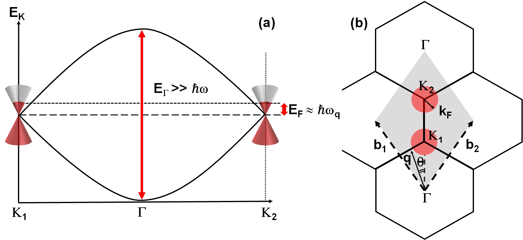
Figure 1: (a) The $\pi$-$\pi*$ electron energy spacing along a straight line from the center to the bounds of a 2D Dirac lattice. The electron energy spacing at the zone center is much larger than the phonon energy making the electron-phonon interactions impossible. The electron energy spacing decreases and becomes comparable to the phonon energy as we move toward the lattice zone boundaries making the electron-phonon interactions possible. (b) The reciprocal lattice of a honeycomb structured lattice is shown as the grey-shaded region where we have two Dirac cones in which electron-phonon interactions take place at.

To derive an analytical expression for the Lindhard dielectric response function we must solve the difference between the occupation number of the levels above and below the Fermi energy, which is provided by the Fermi Dirac statistics in the numerator of the integral in Eq.(2) by applying a suitable approximation. The most used approximation for simplifying the Fermi-Dirac distribution function is the “single step” function used at $\mathrm{T}\approx 0$ K where the Fermi-Dirac distribution has a value of 1 for energies below the Fermi energy, and a value of 0 for energies above.[pathria2016statistical] However, at finite temperatures the “single step” function approximation is no longer accurate since the distribution gets smeared out, as some electrons begin to be thermally excited to energy levels above $E_{\mathrm{F}}$. We, therefore, approximate the Fermi-Dirac distribution with a “double step” function which has three values 1, 1/2, and 0 and covers the distribution of electrons at different energies more accurately, shown in Fig. 2(a). Furthermore, while at T = 0 K the chemical potential $\mu$ is equal to $E_{\mathrm{F}}$ this is no longer the case at finite temperatures where $\mu$ becomes dependent on both $E_{\mathrm{F}}$ and T. Therefore, to find the values of the Fermi-Dirac distribution function at different energies using the “double step” function we must find a relation between $\mu$, $E_{\mathrm{F}}$ and T.

In metals where we have large free electron density in the proximity of the Fermi energy $E_{\mathrm{F}}$, we use the Sommerfeld expansion to write the chemical potential, $\mu$, as a function of $E_{\mathrm{F}}$ and T [ashcroft2001festkorperphysik]. However, Sommerfeld expansion cannot be reliable for 2D Dirac crystals which have a limited concentration of free electrons and we need to express small fluctuations of $\mu$ over $E_{\mathrm{F}}$. Therefore, to write $\mu$ in terms of $E_{\mathrm{F}}$ and T for 2D Dirac crystals we have to develop a new relation. To this end, we define $\Delta E_{\pm}$ to be the range of the singly occupied energy levels in the Dirac cone situated above and below the Fermi energy, respectively, shown in Fig. 2(b). The integrated density of states over $\Delta E_{\pm}$ are equal and are defined as $\Delta g_{\pm\mathrm{(T)}}$. By analyzing Fig. 2(b) we can write $\mu$ as a function of $E_{\mathrm{F}}$ and $\Delta E_{\pm}$ in the following manner:

$$\mu=E_{F}+\frac{\Delta E_{+}-\Delta E_{-}}{2}.$$ (3)

To write $\Delta E_{\pm}$ in terms of $E_{\mathrm{F}}$ and T we first write the sum of the singly occupied energy levels in the Dirac cone situated above and below the Fermi energy level, Fig. 2(b), as follow:

$$\Delta E_{+}+\Delta E_{-}=k_{B}\mathrm{T}.$$ (4)

We further know that the integrated density of states over $\Delta E_{+}$ and $\Delta E_{-}$ are equal. This results in the surface area of the two red and blue regions on the Dirac cone in Fig. 2(b) to be equal to one another and result in the following equation:

$$\Delta E_{-}(2E_{\mathrm{F}}-\Delta E_{-})=\Delta E_{+}(2E_{\mathrm{F}}+\Delta E_{+}).$$ (5)

By inserting Eq.(4) into Eq.(5) we find a relation between $\Delta E_{\pm}$ and $E_{\mathrm{F}}$ and T. We can therefore write the chemical potential as:

$$\mu(E_{\mathrm{F}},\mathrm{T})=E_{\mathrm{F}}+\frac{\Delta E_{+}-\Delta E_{-}}{2}=\sqrt{\Big{|}E_{\mathrm{F}}^{2}-\Big{(}\frac{k_{B}\mathrm{T}}{2}\Big{)}^{2}\Big{|}}.$$ (6)

To find the difference between $f_{\boldsymbol{\xi}+\psi/{2}}$ and $f_{\boldsymbol{\xi}-\psi/{2}}$ versus the energy we use a “double step” function approximation as shown in Fig. 2(a). By computing the area under the curve for the two occupation levels shown in Fig. 2(c) we have:

$$f_{\boldsymbol{\xi}+\frac{\psi}{2}}-f_{\boldsymbol{\xi}-\frac{\psi}{2}}=\left\{\begin{array}[]{ll}``1/2"&\sqrt{\Big{|}E_{\mathrm{F}}^{2}-\Big{(}\frac{k_{B}\mathrm{T}}{2}\Big{)}^{2}\Big{|}}-\frac{k_{B}\mathrm{T}}{2}-\frac{cq}{2}<E_{\xi}<\sqrt{\Big{|}E_{\mathrm{F}}^{2}-\Big{(}\frac{k_{B}\mathrm{T}}{2}\Big{)}^{2}\Big{|}}-\frac{k_{B}\mathrm{T}}{2}+\frac{cq}{2}\\ ``1/2"&\sqrt{\Big{|}E_{\mathrm{F}}^{2}-\Big{(}\frac{k_{B}\mathrm{T}}{2}\Big{)}^{2}\Big{|}}+\frac{k_{B}\mathrm{T}}{2}-\frac{cq}{2}<E_{\xi}<\sqrt{\Big{|}E_{\mathrm{F}}^{2}-\Big{(}\frac{k_{B}\mathrm{T}}{2}\Big{)}^{2}\Big{|}}+\frac{k_{B}\mathrm{T}}{2}+\frac{cq}{2}\end{array}\right.$$ (7)

Where the energy bounds in Eq.(7) for which $f_{\boldsymbol{\xi}+\psi/{2}}-f_{\boldsymbol{\xi}-\psi/{2}}=1/2$ is shown by the purple shaded region in Fig. 2(c). The difference between the two, sets the bounds of integration for calculating the dielectric response function at non-zero temperature. By analyzing Eq.(7) at $\mathrm{T}\approx 0$ K we observe that the two purple regions in Fig. 2(c) overlap with one another, and the “double step” function turns into a “single step” function further confirming our results.

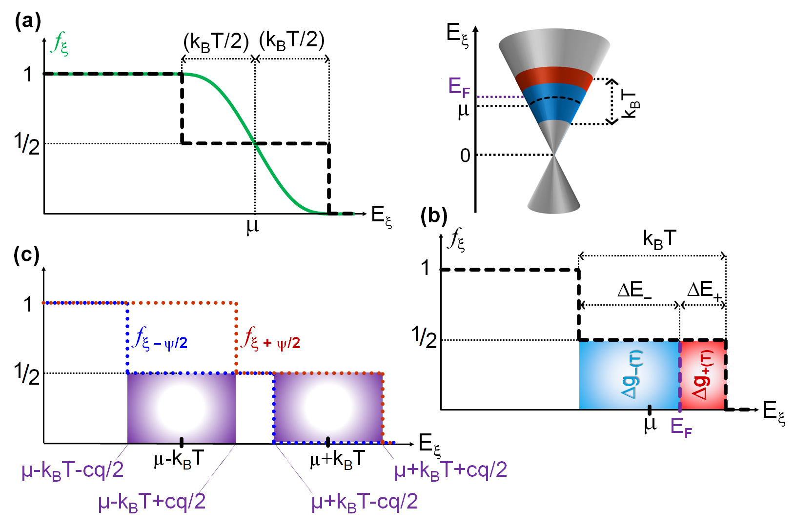
Figure 2: (a) “Double step” approximation of the occupation function of an electron used in this paper to calculate the dielectric response function for $\mathrm{T}\neq 0$ K. (b) The “double step” approximation and the Dirac cone of a 2D crystal with an elevated Fermi energy level $E_{\mathrm{F}}$. Areas of the Dirac cone highlighted in red and blue lead to equal number of states at energy ranges $\Delta E_{+}$ and $\Delta E_{-}$ above and below $E_{\mathrm{F}}$, respectively. (c) The difference between $f_{\boldsymbol{\xi}+\psi/2}$ and $f_{\boldsymbol{\xi}-\psi/2}$ as a function of energy in a 2D Dirac crystal shown in the two purple squares which set the bounds of integration for calculating the dielectric response function.

By raising the temperature, the Fermi energy of the 2D Dirac crystal shifts leading the bounds of the integration in Eq.(2) for the dielectric response function to also change. While the bounds of the integration for $\xi(\psi,\omega)$ at T = 0 K are between $1/2\pm\psi/2$, using the “double step” function to derive the difference in the Fermi-Dirac distribution for $\mathrm{T}\neq 0$ K we have:

$$\begin{split}\chi(\psi&,\omega)=-\frac{e^{2}}{4\pi^{2}}\\ &\Bigg{(}\int_{\frac{\mu}{2E_{\mathrm{F}}}-\frac{\tau}{2}-\frac{\psi}{2}}^{\frac{\mu}{2E_{\mathrm{F}}}-\frac{\tau}{2}+\frac{\psi}{2}}d\xi_{x}\int_{\xi_{y,min}}^{\xi_{y,max}}\frac{d\xi_{y}}{E_{\boldsymbol{\xi}+\frac{\psi}{2}}-{E_{\boldsymbol{\xi}-\frac{\psi}{2}}}-cq}+\int_{\frac{\mu}{2E_{\mathrm{F}}}+\frac{\tau}{2}-\frac{\psi}{2}}^{\frac{\mu}{2E_{\mathrm{F}}}+\frac{\tau}{2}+\frac{\psi}{2}}d\xi_{x}\int_{\xi_{y,min}}^{\xi_{y,max}}\frac{d\xi_{y}}{E_{\boldsymbol{\xi}+\frac{\psi}{2}}-{E_{\boldsymbol{\xi}-\frac{\psi}{2}}}-cq}\Bigg{)}.\end{split}$$ (8)

Where we have written the dielectric response function in dimensionless coordinates as $\chi(\psi,\omega)=\chi(q,\omega)/2k_{\mathrm{F}}$. We see that by approximating the occupation function of the electron with a “double step” function we split the integral in Eq.(2) into two integrals where the bounds of each integral is one of the purple shaded regions depicted in Fig. 2(c).

A disadvantage of the Lindhard model over more simplistic approximations such as Thomas-Fermi, is the requirement of carrying out integrations that often cannot be performed analytically, and may become cumbersome where: $i)$ the model is dynamic–i.e. one assumes that phonons not only carry momentum, but also energy $\hbar\omega_{0}$; or $ii)$ nonzero temperature is considered–a necessary requirement to compare $\chi(q)$ with experiments involving, for example, T-dependent electrical or transport measurements; or $iii)$ the phonon energy $\hbar\omega_{q}$ is wavevector-dependent in a dispersive system–a respect in which it is worthwhile noting that the phonon energy is not only required in dynamic Lindhard-model calculations but also static ones, as it affects the electron Fermi-Dirac distribution, also at 0 K. Of course, the complexity of the calculation will increase if more than one of the phenomena $(i-iii)$ are considered. To simplify the integral we assume the extreme carrier mobility in 2D Dirac crystals results in their Fermi velocity to be much larger than the speed of sound, $\mathrm{v}_{\mathrm{F}}>>c$. This has been experimentally confirmed in various 2D Dirac crystals such as graphene[hwang2012fermi], borophene[xu2016hydrogenated], Weyl semimetals[lee2015fermi], and silicene[kara2012review] where $c<0.01\mathrm{v}_{\mathrm{F}}$. Defining $\mathrm{w}_{\mathrm{F}}=c/\mathrm{v}_{\mathrm{F}}$ we can expand the dielectric response function around $\mathrm{w}_{\mathrm{F}}$ with $\mathrm{w}_{\mathrm{F}}\to 0$ in the following manner:

$$\chi {}_{\mathrm{w}{}_{\mathrm{F}}}(\psi )=\chi {}_0(\psi )+$$ (9)