Evidence of Periodic Variability in $\gamma$-ray Emitting Blazars with Fermi-LAT

Abstract

It is well known that blazars can show variability on a wide range of time scales. This behavior can include periodicity in their $\gamma$-ray emission, whose clear detection remains an ongoing challenge, partly due to the inherent stochasticity of the processes involved and also the lack of adequately-well sampled light curves. We report on a systematic search for periodicity in a sample of 24 blazars, using twelve well-established methods applied to Fermi-LAT data. The sample comprises the most promising candidates selected from a previous study, extending the light curves from nine to twelve years, and broadening the energy range analyzed from $>$1 GeV to $>$0.1 GeV. These improvements allow us to build a sample of blazars that display a period detected with global significance $\gtrsim 3\,\sigma$. Specifically, these sources are PKS 0454$-$234, S5 0716+714, OJ 014, PG 1553+113 and PKS 2155$-$304. Periodic $\gamma$-ray emission may be an indication of modulation of the jet power, particle composition, or geometry, but most likely originates in the accretion disk, possibly indicating the presence of a supermassive black hole binary system.

1 Introduction

Active Galactic Nuclei (AGN), i.e. galaxies with an accreting supermassive black hole (SMBH) in the center, are among the most luminous persistent objects in the Universe (e.g.,  Soltan,, 1982; Cavaliere and Padovani,, 1989; Witta,, 2006). The complex interplay between the black hole hosted at the AGN core and the surrounding circumnuclear gas leads to the formation of an accretion disk and may influence the properties of the host galaxy (e.g., the stellar mass of the inner bulge, Haring and Rix,, 2004). A small fraction of AGN is distinguished by the presence of a pair of highly collimated, relativistic jets. These jets typically form in opposite directions, perpendicular to the rotational plane of the SMBH-accretion disk system. When one of the jets is closely aligned with the line of sight, the object is referred to as a blazar. The observed emission from blazars is strongly dominated by the jet, spans energies ranging from radio to $\gamma$-rays, and can be highly variable on time scales ranging from seconds to years (e.g., Urry,, 1996, 2011).

During their cosmological evolution galaxies can merge (e.g., Jiang et al.,, 2012), frequently at moderate/high redshifts (e.g., Rieger,, 2007; Lin et al.,, 2008) when they are also more gas-rich (e.g., Tacconi,, 2010). In the process of a AGN merger, one expects that the two SMBHs hosted at the respective centers eventually meet and form a binary system with a typical separation of about kiloparsec (Begelman et al.,, 1980). Such a binary system is referred to as supermassive black hole binary (SMBHB). As a consequence of dynamical friction, the SMBHs can converge to the center of mass of the galaxy and shrink their separation down to sub-parsec distances (e.g., Dosopoulou and Antonini,, 2017). Finally, the last stage of merging is the coalescence of the SMBHBs into a single SMBH (e.g., Colpie,, 2014), resulting in one of the loudest sources of gravitational waves in the Universe (e.g., Enoki et al.,, 2004).

The identification of SMBHB systems with sub-parsec separation is an important topic of astrophysics but remains challenging since they cannot generally be spatially resolved and because they are rare. Limits on the nanohertz stochastic gravitational wave background from the Pulsar Timing Array (PTA, Holgado et. al,, 2018; Rieger,, 2019) suggest that only a minor fraction ($\lesssim\,$0.01–0.1%) of blazars could be harboring SMBHBs with sub-parsec separations (e.g., Liu et al.,, 2014). Such SMBHBs could imprint peculiar time-variability patterns in their emitted radiation with periods of on the order of one year.

One of the strategies employed to pinpoint candidate SMBHBs has been the search for periodic modulation, also known as quasi-periodic oscillations, in AGN light curves (LCs). The detection of periodicity in blazars has been limited by the lack of continuous and sensitive long-term sampling. Recently, the Large Area Telescope (LAT) on board the Fermi Gamma-ray Space Telescope has alleviated this issue by scanning the entire sky regularly with high sensitivity (Atwood et al.,, 2009). During more than a decade of continuous monitoring since Fermi was launched in 2008, the LAT has collected a wealth of valuable data, offering the unprecedented opportunity to monitor flux variations from thousands of blazars in the GeV band. Densely sampled, unbiased, high-quality LCs are now accessible for all sources in the LAT catalogs. The fourth $Fermi$-LAT source catalog (4FGL, Abdollahi et al.,, 2020; Ballet et al.,, 2020) is based on the first 8 years of LAT observations and includes more than 5000 sources, among which about 3000 are confidently associated with blazar counterparts. Recently, the 4FGL-DR3 catalog has been published, which is based on the first 12 years of LAT observations (Abdollahi et al.,, 2022).

Searching for periodicity in a time series (an ordered sequence of fluxes as a function of time) requires measuring the power of the time series at each frequency and identifying the dominant frequency, if any. This information is captured in periodograms, which are obtained through a variety of techniques such as Lomb-Scargle (Lomb,, 1976; Scargle,, 1982) and wavelets (Torrence and Compo,, 1998; Foster,, 1996). For the most part, studies in the literature that search for periodicity in blazar $\gamma$-ray LCs have mainly focused on a few selected objects and typically have employed at most two or three time-series algorithms (e.g., Tavani et al.,, 2018; Zhang et al., 2017a, ; Bhatta and Dhital,, 2020). These previous studies found a few candidates with periodicity (e.g., PG 1553+113 or OJ 287, Ackermann et al.,, 2015; Valtonen et al.,, 2016, respectively) but due to the stochastic nature of emission in blazars, these findings remain under debate (e.g., Covino et al.,, 2019). As a pioneering investigation in Peñil et al., (2020, P20, hereafter), we performed a comprehensive search for periodicities in blazar $\gamma$-ray LCs, targeting $\sim$2,000 blazars and adopting ten of the most used methods for time-series analysis. Our effort discovered 24 periodic blazar candidates with local (pre-trial) significance above $3\sigma$.

In the work presented here, we reanalyze the 24 candidates from P20, employing new data that cover three additional years of Fermi-LAT observations. We apply a similar periodicity-detection pipeline as the one described by P20 and include new statistical methods. Specifically, we also use the autoregressive models Autoregressive Integrated Moving Average (ARIMA) and Autoregressive Fractionally Integrated Moving Average (ARFIMA) to deal with the stochastic uncertainty introduced by noise in the periodicity search. Finally, we also take into account the look-elsewhere effect to provide robust significances for the detected periods.

The paper is organized as follows. In $\S$2, the blazar sample and data reduction methodology are presented. Then, $\S$3 details the periodicity analysis methodology and $\S$4 shows and discusses our results. In $\S$5, there is a description of the potential interpretation of the results focusing on the two sources with the most significant periodicity. We summarize the findings in $\S$6.

2 $\gamma$-ray sample

2.1 Fermi-LAT data reduction

The $Fermi$-LAT data are reduced with the Python package fermipy (Wood et al.,, 2017). The following procedure is adopted for each source in the sample. We select photons of the Pass 8 SOURCE class (Atwood et al.,, 2013; Bruel et al.,, 2018), in a region of interest (ROI) of 15^∘ $\times$ 15^∘ square, centered at the target. To minimize the contamination from $\gamma$ rays produced in the Earth’s upper atmosphere, a zenith angle cut of $\theta<90^{\circ}$ is applied. We also applied the standard data quality cuts ($\rm DATA\_QUAL>0)\&\&(LAT\_CONFIG==1$) and removed time periods coinciding with solar flares and $\gamma$-ray bursts detected by the LAT. The ROI model includes all 4FGL catalog sources (Abdollahi et al.,, 2020) located within 20^∘ from the ROI center, as well as the Galactic and isotropic diffuse emission (gll_iem_v07.fits and iso_P8R3_SOURCE_V6_v06.txt).

We perform a binned analysis in the 0.1-800 GeV energy range, using 10 bins per decade in energy and 0.1^∘ spatial bins, and adopting the P8R3_SOURCE_V2 instrument response functions. First, a maximum likelihood analysis is performed over the full time range considered here, i.e. 2008 Aug 04 15:43:36 UTC to 2020 Dec 10 00:01:26 UTC. In the fit, we model the sources in the ROI, adopting the spectral shapes and parameters reported in 4FGL. We allow the normalization and spectral index of the target source to vary, as well as the normalizations of all sources within 3^∘ of the ROI center and the isotropic and Galactic diffuse components. Since our data span a different integration time with respect to 4FGL, our first results are checked for potential newly-detected sources with an iterative procedure. To this aim, a test statistic (TS) map is produced. The TS is defined as $2\log(L/L_{0})$, where $L$ is the likelihood of the model with a point source at a given position and $L_{0}$ is the likelihood without the source. A TS value of 25 corresponds to a statistical significance of $\gtrsim 4.0\sigma$ (according to the prescription adopted in Abdollahi et al.,, 2020; Mattox, et al., 1996). A TS map is produced by including a putative point source at each pixel of the map and evaluating its significance over the current best-fit model. The test source is modeled with a power-law spectrum where only the normalization is allowed to vary in the fit, whereas the photon index is fixed at 2. We look for significant peaks (TS$>$25) in the TS map, with a minimum separation of 0.5^∘ from existing sources in the model, and add a new point source to the model at the position of the most significant peak found. Then, the ROI is fitted again, and a new TS map is produced. This process is iterated until no more significant excesses are found, generally leading to the addition of two point-sources.

In order to produce the LCs, we split the data for each source into 28-day bins and perform a full likelihood fit in each time bin. For the likelihood fits of the time bins, the best-fit ROI model obtained from the full time-interval analysis is adopted. We first attempt a fit allowing variation in the normalizations of the target and of all sources in the inner $3^{\circ}$ of the ROI, along with the diffuse components. If the fit does not converge, the number of free parameters is progressively restricted in the fit in an iterative way until the fit successfully converges. We begin this iterative process by fixing sources in the ROI that are weakly detected (i.e., with TS$<$4). Next, we fix sources with TS$<$9. Then, we fix sources up to $1^{\circ}$ from the ROI center and those with TS$<$25. Finally, we fix all parameters except the target source’s normalization. We consider the target source to be detected when TS$>$1 in the corresponding time bin. Whenever this condition is not fulfilled, a 95% confidence upper limit is reported from the likelihood distribution (these points are denoted by down arrows in the plots of the LCs).

2.2 Source selection

The blazar sample in P20 was analyzed using 9 years of Fermi-LAT observations (see Table 1). In this work we reanalyze the 24 periodicity candidates pinpointed in P20 in a similar way but with several improvements:

1. Extend the observing time to 12 years, from August 2008 until December 2020.

2. Expand the energy range from $\rm{>1}$ GeV to $\rm{>0.1}$ GeV, thus increasing the photon statistics, improving the signal-to-noise ratio, and dramatically reducing the number of upper limits in the LCs. For example, S4 1144+40 had a fraction of 40% upper limits in P20, which is reduced to $<$1% here.

3. Retain the information for the LC points with low statistics (i.e., non-detection) by substituting the upper-limit data with the value of the flux that maximizes the likelihood function for that time bin.

We use the same 28-days binning for the LCs. This time binning provides an adequate compromise between a computationally manageable analysis and sensitivity to long-term variations (of the order of a year).

3 Methodology

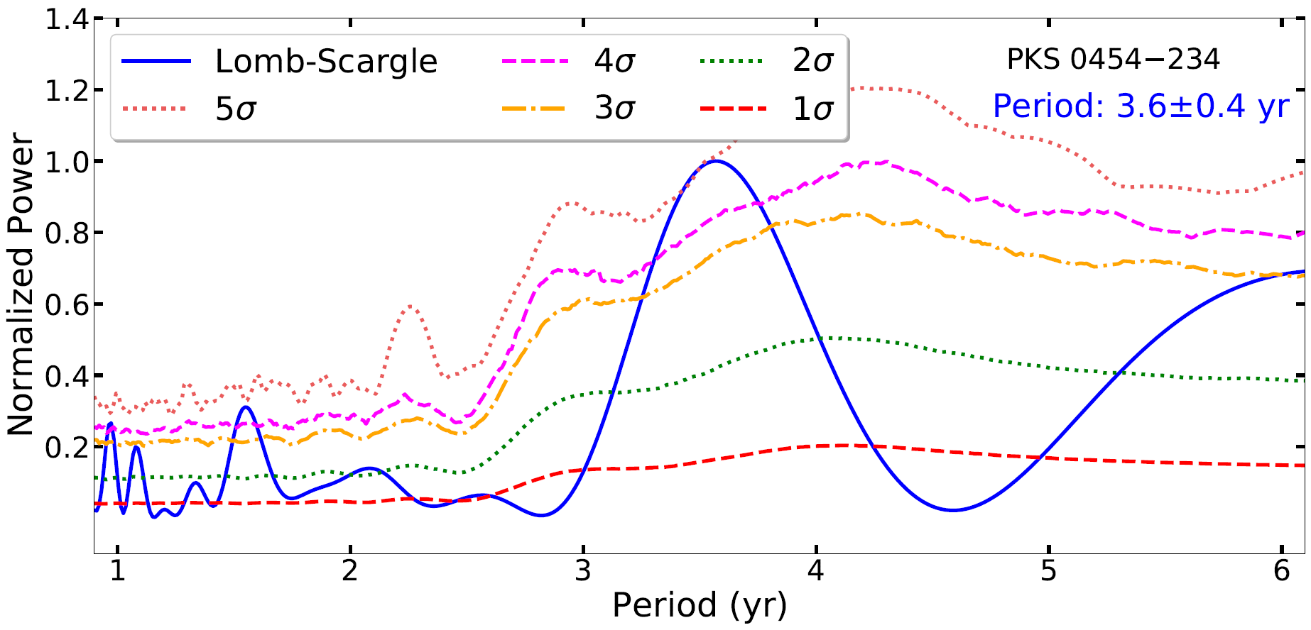
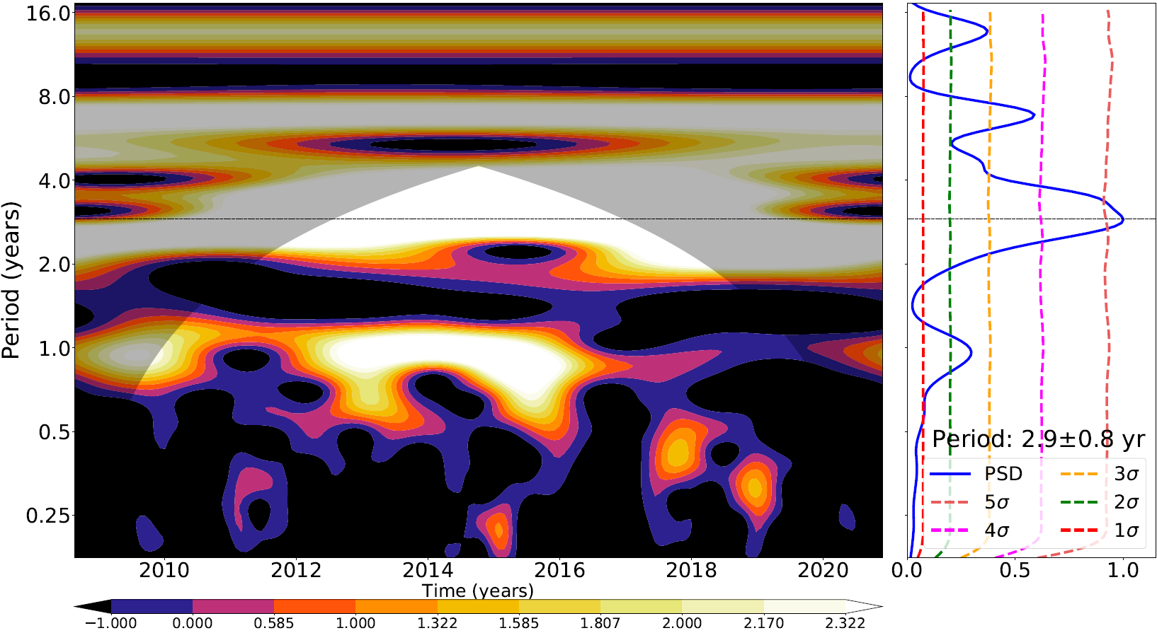
Figure 1: Examples of the application of two methods for the search of periodicity. Left: Lomb-Scargle periodogram (Lomb,, 1976; Scargle,, 1981) for PKS 0454$-$234, showing a significant peak at a $\sim$3.6 yr period. The significance levels were obtained by simulating artificial LCs based on the technique from Emmanoulopoulos, (2013). Right: results from continuous CWT for S5 0716$-$71. The colormap shows the periodicity information as a function of time, where the color represents the PSD of the signal, identifying patterns and scales in variability, highlighting the presence of any period in the signal. The cone of influence (captured by the shaded section) denotes where putative modulations are either too close to the sampling interval or too close to the total signal length. To the right of the colormap is a periodogram, and significance levels are indicated (also obtained with by simulating artificial LCs). A significant peak is observed at a $\sim$2.9 yr period, which is present during the twelve years of the light curve. A secondary periodicity of $\sim$1 yr is detected with $2.5\sigma$ significance. This putative $\sim$1 year period is weakly represented in the first eight years of the light curve, as can be seen in the colormap.

3.1 Periodicity search methods

Periodicity searches are limited in part by noise. Many Galactic and extragalactic astrophysical sources show erratic brightness fluctuations with steep power spectra (e.g.,  Gao et al.,, 2003). In this context, the noise is defined as random variations in the source emission. Noise is classified according to the power-law index $\beta$ of the power spectral density (PSD, $\propto f^{-\beta}$ where $f$ is frequency, Rieger,, 2019). The PSD measures the power in a signal as a function of the frequency. White, pink, and red noises are characterized by indices of $\beta\!=\!0$, $\beta\!=\!1$, and $\beta\!=\!2$, respectively (e.g.,  Tarnopolski,, 2020).

We search for long-term ($\sim$years) periodicity since we are looking for blazars to be SMBHB candidates in the gas-driven regime (see $\S$5). Consequently, we choose to search for periods in the [1-6] year range.

While a study of shorter periods (e.g., $\sim$months) would suffer less contamination due to red noise, other challenges appear. First, the smaller bins contain fewer $\gamma$-ray photons, so the statistical uncertainty per bin is larger. Second, in the context of searching for binaries, the residence time at a given orbital period $t_{\rm orb}$ scales as $t_{\rm orb}^{8/3}$ in the gravitational wave-driven regime (Haiman et al.,, 2009). Thus, considering month-long periods rather than year-long periods would reduce the expected number of binaries in the sample by more than 99%. On the other hand, this also implies that any periodicity found shorter than $\sim$year-long is more likely to be due to other processes, e.g. disk and/or jet procession from a single SMBH. These alternative processes are interesting in their own right, and we intend to explore shorter periods in future works.

Careful considerations must be taken in a periodicity-search analysis. In general, each method has specific properties, e.g., accuracy, computational time, sensitivity to irregular time series, among others. Therefore, the selection of just one time-series method is arguably arbitrary, since all have limitations and advantages (Goyal et al.,, 2017; VanderPlas,, 2018). In light of this, we employed in P20 and here ten of the most widely used methods for periodicity identification in order to reduce the impact of their individual limitations and take advantage of their individual strengths (see Figure 1). These methods are listed below:

1. Lomb-Scargle periodogram (LSP, Lomb,, 1976; Scargle,, 1982).

2. LSP superposed on a red noise spectrum (Vaughan,, 2005).

3. Generalized Lomb-Scargle periodogram (GLSP, Zechmeister and Kürster,, 2009).

4. Phase Dispersion Minimization (PDM, Stellingwerf,, 1978).

5. REDFIT (Schulz and Mudelsee,, 2002).

6. Enhanced Discrete Fourier Transform improved by applying Welch’s method (DFT, Welch,, 1967).

7. Continuous Wavelet Transform (CWT, Torrence and Compo,, 1998).

8. Weighted Wavelet Z-transform (WWZ, Foster,, 1996). We do not use this method in this work since the LCs analyzed are evenly-spaced time series. In this case, CWT reports consistent results to WWZ.

9. Markov Chain Monte Carlo Sinusoidal Fitting (MCMC Sine, Foreman-Mackey et al.,, 2018).

10. Bayesian quasi-periodic oscillation (Huppenkothen et al.,, 2013).

To complement these, we use techniques to infer the significance of the periods found by the search algorithms. For instance, we use the strategy described by Emmanoulopoulos, (2013), which allows generating LCs with the same PSD and the same probability density function as real blazar LCs. Following Emmanoulopoulos, (2013), we generate LCs by applying the bending-power law approach, which allows us to have the correct amount of power at both low and high frequencies (dominated by white and red noise, respectively). Therefore, this approach provides realistic models of blazars’ variability on timescales from weeks to years (Chakraborty and Rieger,, 2020).

All of these methods and techniques are organized in a pipeline described in P20, to which we refer the reader for further details. In this current work, we adopt the same pipeline, except for the addition of new methods, which are described in the following sections.

3.2 Autoregressive models

In this work, we include autoregressive models to improve our analysis pipeline. These models are proposed as efficient methods for astronomical data analysis, particularly to infer any periodic behavior (Scargle,, 1981; Caceres,, 2019). To analyze the Fermi-LAT LCs, the ARIMA (Chatfield,, 2003) and ARFIMA (Feigelson,, 2018) are applied. These autoregressive models are suitable for analyzing astronomical time series since they allow modeling a wide variety of LC properties (e.g., irregular or quasi-periodic, constant mean or variable mean) or combinations of stochastic and deterministic behaviors (Feigelson,, 2018). These characteristics make these models more robust against stochastic noise, helping to infer periodic behaviors more accurately (Caceres,, 2019).

Both models are based on an auto-correlation (correlation of the LC with itself) where one looks for dependencies of the current values (of the LC) on past values. In this approach, the current values are modeled as the sum of two linear combinations of past values (with $p$ and $q$ terms, respectively) that model an autoregressive and stochastic process, respectively (see Feigelson,, 2018, for details). The parameter $d$ in ARIMA represents how stationary the LC is, i.e., whether a time series has a constant mean and variance (in which case, $d$=0). In ARFIMA, the parameter $d$ represents the type of process. For instance, 0$<d<$1 corresponds to a long memory process, while -0.5$<d<$0 is a short memory process. This parameter is in the 0-0.5 range for a stationary time series. A stochastic process is modeled as ARFIMA(1,d,0) (Xu,, 2019), and ARIMA(0,0,1) (Zhang et al.,, 2020).

The ARFIMA model can be applied to stationary time series. Stationarity is measured using the augmented Dickey-Fuller unit root test (Dickey and Fuller,, 1979), which tests the null hypothesis that a time series is non-stationary. For the purposes of this study, we reject the null hypothesis if the p-value is $\rm{\leq 0.05}$. If the mean and variance are not constant, we apply the ARIMA model instead, which can deal with this scenario (see e.g.  Caceres,, 2019).

The periodicity search with these methods begins with selecting the best-fit ARFIMA/ARIMA model using Akaike’s Information Criterion (AIC,  Akaike,, 1973). The AIC is a statistical estimator to evaluate a model fit to the data. AIC is used to compare models to determine which one performs the best fit for the data. After that, the residuals are obtained from the original LC and the selected ARFIMA/ARIMA model. Then, we compute the Autocorrelation Function (ACF) on these residuals (see Figure 2). We use the same criterion presented in the literature by using a $\rm{\geqslant 2\sigma}$ threshold for significance (e.g.,  Zhang et al., 2017c, ; Zhang et al.,, 2020; Yang et al.,, 2021). Finally, we use the Ljung-Box test to evaluate the quality of fit between the LC and its ARFIMA/ARIMA model (Ljung and Box,, 1978). The Ljung-Box test checks whether or not the autocorrelations for the residuals are non-zero, denoting the lack (or not) of model fit. We consider the fit to be adequate when the p-value is at least 0.05. Note that higher p-values mean that the ARFIMA/ARIMA model fits the LC better.

To implement the ARFIMA/ARIMA analysis, we use the R packages stats and arfima. This R functionality is accessible from a Python environment via the package rpy2.

4 Results and discussion

We run the LCs of our 24 blazars through our improved pipeline. The results of the analysis are listed in Table 2 and Table 3.

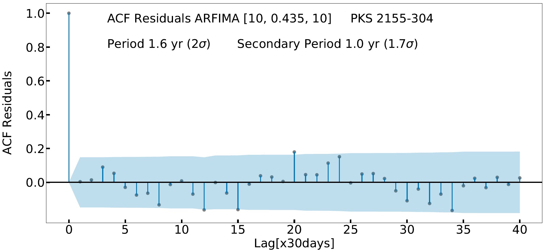
Figure 2: Correlation of the residuals (between the LC and the ARFIMA [p=10, d=0.453, q=10] model) for PKS 2155$-$204. The colored area represents the 2$\sigma$ confidence level. The peak at zero lag represents the autocorrelation of the residual with itself.

In order to sort the blazars, we quantify the periodicity significance by computing the median significance across all methods (excluding REDFIT since it gives a maximum significance of 2.5$\sigma$).

4.1 High-significance periodicity candidates

The first group consists of the 5 blazars with periodicity detections at a median significance of $\gtrsim$5 $\sigma$, before the correction described in $\S$4.4 is applied. This sample includes 5 sources, PKS 0454$-$234, S5 0716+714, OJ 014, PG 1553+113, and PKS 2155$-$304 (Figure 3). Three different scenarios arise when applying the ARFIMA/ARIMA methods:

1. The methods find a significant period that is similar (compatible period) to those found via the methods listed in $\S$3 and Table 2 (e.g., PKS 2155$-$304).

2. The modeling provides a compatible period at $\rm{\geq 1.5\sigma}$. (OJ 014, and PG 1553+113, the period of $\approx$2 yr for the latter is observed as a secondary peak).

3. No compatible period is reported for PKS 0454$-$234 and S5 0716+714.

Excluding the ARFIMA/ARIMA analysis, we confirm the period of $\approx$2.7 yr for S5 0716+714 found in P20 and in the recent analysis by Bhatta, (2021). This period differs from the $\approx$ 0.9 yr period reported by Prokhorov and Moraghan, (2017), Li et al., (2018), Sandrinelli et al., (2017), and Bhatta and Dhital, (2020). However, we do report the $\approx$0.9 yr period as a secondary peak (see Table 2). These disagreements may be due to the fact that we use more telescope time (e.g., $\sim$8 yrs in Li et al.,, 2018; Bhatta and Dhital,, 2020) or by the technique employed to infer significances (e.g., Prokhorov and Moraghan,, 2017; Bhatta and Dhital,, 2020).

Regarding PG 1553+113 and PKS 2155$-$304, we confirm our previous period detections (e.g., compatible with Tavani et al.,, 2018; Zhang et al., 2017a, , respectively). For PKS 0454$-$234, Bhatta and Dhital, (2020) do not find any significant detection (note that we use more telescope time, and the significance is obtained differently).

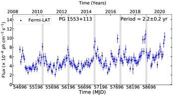
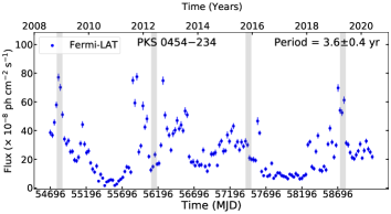
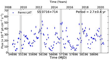
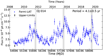
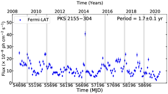
Figure 3: Light curves of the 5$\sigma$ periodicity sample. The gray vertical bars approximate high-flux periods suggested by the period inferred by the methodology for the given blazar. The width of the gray bars indicate the uncertainty in the periodic signal. Note that it is difficult to identify the periodic emission of S5 0716+714 by eye because this source may have two detected periods (see later).

Covino et al., (2019) searched for blazar periodicity in a sample of 10 blazars (including 3 from our high-significance sample: S5 0716+714, PG 1553+113, and PKS 2155$-$304), and they did not find evidence for periodicity. In this case, the different results could be associated with analysis methodology employed in Covino et al., (2019). Ait Benkhali et al., (2020) also reported mild support for periodicity in some of our high-significance candidates.

Our results are in general not consistent with those by Yang et al., (2021, except for PG 1553+113). The reason can be that these authors analyze most of the candidates in P20 using the Continuous-time Autoregressive Moving Average (CARMA). However, according to Feigelson, (2018), the CARMA method assumes weak stationary behavior in LCs without considering any trends in the flux. However, ARFIMA treats such behaviors in the LCs (Feigelson,, 2018). Yang et al., (2021) justify the use of CARMA on the basis that the LCs they analyzed are irregularly sampled (due to the presence of upper limits). But moderately irregular measurements can be treated as evenly-spaced time series with missing data; hence, the ARIMA/ARFIMA models can also be applied and are better than the CARMA models for analyzing blazar LCs.

4.2 Low-significance periodicity candidates

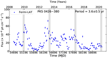
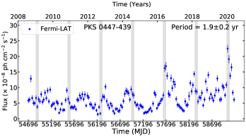
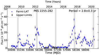
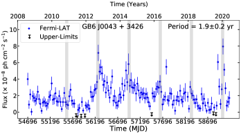
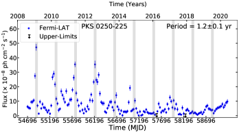
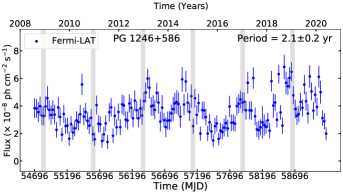
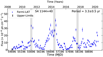
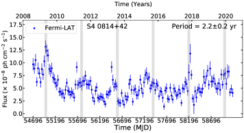
Figure 8: Light curves of the low-significance blazars presented in Table 1. The gray vertical bars approximate high-flux periods suggested by the period inferred by the methodology for the given blazar. The width of the gray bars indicate the uncertainty in the periodic signal.

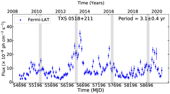
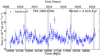
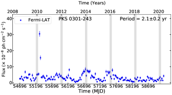
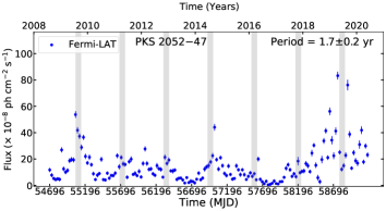
Figure 8: (Continued).

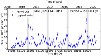
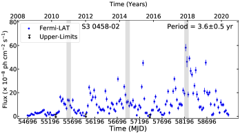
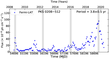
Figure 8: (Continued).

The rest of the sample includes 6 blazars with periods detected at $\rm{\geqslant 4\sigma}$ (PKS 0426-380, PKS 0447-439, PKS 2255-282, GB6 J0043+3426, PKS 0250-225, PG 1246+586; see Table 1 and Figure 8 in the Appendix). We discard 7 candidates with a median significance of $\rm{\leq 2.5\sigma}$ (TXS 1452+516, MG2 J130304+2434, TXS 0059+581, 87GB 164812.2+524023, MG1 J021114+1051, S3 0458$-$02, PKS 0208$-$512). The periods of the blazars presented previously in the literature are mostly compatible with our corresponding results (e.g., PKS 0426$-$380 and MG2 J130304+2434, Zhang et al., 2017b, ; Zhang et al., 2017c, , respectively).

We note that not all of the candidates presented by P20 increased the significance with the additional 3 years of data. For example, large drops in significance were found for MG1 J021114+1051 and TXS 1452+516 (see Table 1).

4.3 Power-spectral index estimation

The PSD can be fitted by a power law according to the expression $\propto\rm f^{-\beta}$, where $\rm f$ is frequency and $\beta$ is the power-law index (e.g.,  Gao et al.,, 2003; Tarnopolski,, 2020). This form for the PSD denotes that $\gamma$-ray variability in blazars is stochastic (e.g.,  Sobolewska et al.,, 2014). Additionally, estimates of the power-law slope provide information about the nature of the variability, denoting the role of the accretion disk in the emission of the jets (e.g.,  Bhatta and Dhital,, 2020). The power spectral index is estimated using the algorithm presented by Uttley et al., (2002), the Power Spectrum Response Method (PSRESP). PSRESP also provides the uncertainty of the estimated slope and the “success fraction” that indicates the goodness of fit by giving the probability of a model being accepted (see Figure 4). To implement PSRESP for each candidate, we simulate 1,000 artificial LCs using the technique of Timmer and Koenig, (1995), generating LCs according to a power-law model with the same observational properties of the original LC (e.g., mean, standard deviation, flux distribution). Additionally, we use a binning of $\sim$0.05 for the estimate of the power spectral index. Note that larger bin sizes may reduce the accuracy of this index derivation. Although we concentrate on periods between 1 year and 6 years, the fits to the PSD index are made over the full frequency range spanned by the LCs.

The results obtained for the candidates are shown in Table 4. The estimated slopes for the power spectrum of our candidates are in the range of [0.9$-$1.5]. This range is compatible with the values proposed in the literature (e.g.,  Nakagawa and Masaki,, 2013; Sobolewska et al.,, 2014; Kushwaha et al.,, 2017; Bhatta and Dhital,, 2020). However, the obtained slopes are $\pm$30% different than those reported by Yang et al., (2021). Ait Benkhali et al., (2020) reported different power spectral indices related to several of our blazars, except for PKS 2155$-$304 with a compatible $\rm\beta\approx 1$. In Table 4, the mean of the slopes for all candidates is $\sim$1.2 with a standard deviation of 0.4. These slopes are compatible with those from Bhatta and Dhital, (2020).

Most of the power-law indices shown in Table 4 are consistent with a pink-noise process (spectral index $\approx$1), which may be caused by disk modulations that materialize as jet modulations. (Bhatta,, 2022).

This process can be associated with short time-scale variability in the periodic baseline (associated with sporadic flaring activity, which might indicate instabilities and turbulence in the accretion flow through the disc or in the jet, Abdo et al.,, 2010). Additionally, a pink-noise process can also be associated with long-term variability that is coherent on time scales on the order of decades (Bhatta and Dhital,, 2020). For example, a process that can produce stochastic emission at both short and long timescales is magnetic reconnection (Bhatta and Dhital,, 2020). In addition to that, variable accretion with large accretion episodes ($\approx$50$–$200 ${{\rm M}_{\odot}}$ yr^-1) followed by smaller ones can also explain PSDs with indices of $\approx$1 (Jolley et al.,, 2009).

Czerny et al., (2004) present a modeling of the relationship between instabilities in the accretion disk and variability, in which the time scales of these instabilities range from hours to a few years for blazars with BH masses of $10^{8}$$-$$10^{9}{{\rm M}_{\odot}}$. For instance, these accretion episodes can be associated with a steep power-law index (red noise, with a spectral index $\approx$2), which produces a dominance of the long-term variability in the LC (e.g., Kunjaya et al.,, 2011). This scenario may be applicable to PKS 0208$-$512 (with a power-law index of 1.6$\pm$0.4).

Alternatively, Goyal, (2018) presents a model to interpret the different timescales observed in the multiwavelength variability of blazars. The variability of the synchrotron emission is powered by a stochastic process with a duration from minutes to years. Regarding the variability of the inverse Compton emission, it results from two stochastic processes, which are linearly overlapping with a duration from one to thousands of days. These two processes are the dissipation in the magnetic field of the jet and inhomogeneities in the number of the photons for the inverse-Compton process.

Finally, Rieger, (2019, and references therein) propose a model of the dominant radiation processes. Specifically, the slope of the PSD depends on the component that dominates the high-energy emission—external Compton or synchrotron self-Compton (with a slope of $\gtrsim 2.0$ signifying the former process).

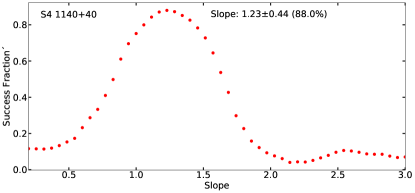
Figure 4: Estimation of the power spectral index for S4 1144+40 using PSRESP. The figure shows the inferred index, the uncertainty, and the “success fraction” associated with the estimation.

4.4 Global significance

In our periodicity analysis, there was no prior knowledge of the frequencies of the potential signal. In these conditions, it is statistically more rigorous to employ a “global significance” (e.g., Ait Benkhali et al.,, 2020). This significance accounts for the look-elsewhere effect, which is the ratio between the probability of observing the excess at some fixed value and the probability of observing it anywhere in the value range considered in the analysis (Gross and Vitells,, 2010). The “global significance” is obtained by applying a correction to the “local significance”, which is the significance of the periodicity in an LC at a specific value that is obtained for each method. This correction is estimated by

$$p_{\mathrm{global}}=1-(1-p_{\mathrm{local}})^{N},$$ (1)

where $N$ is the trial factor. In our study, we have to consider two potential issues. One is that we do not know the frequency for each source a priori, so we must search for the highest peak in each of the periodograms. The second issue is that we do not know a priori which sources exhibit periodic behavior, so we must select them from the periodograms, as well. Consequently, searching $P$ independent periods (frequencies) in each of the periodograms of $B$ blazars, the number of trials is

$$N=P\times B.$$ (2)

We do not consider the number of methods in the trials since we present all the results for all the methods equally in our tables for each blazar, avoiding picking the highest significant result according to a single method.

In P20, we analyzed $\approx$2000 blazars; however, after eliminating blazars for which $\geqslant$50$\%$ of the LCs consist of upper limits, the number of blazars included in our sample was 351. There is no unique way to determine $P$ in a given periodogram. For instance, Zechmeister and Kürster, (2009) set $P$ based on the frequency range and resolution considered in the periodicity analysis. In our periodograms, we have followed this approach, considering 100 periods (to have a good balance between computational time and resolution in the periodograms). However, for a 12-year LC with $\approx$12 samples/year (for approximately $M=144$ points in the LC), our period range ([1-6] years) corresponds to 11 independent frequencies sampled. These frequencies are obtained from the expression,

$$f_{j}=\frac{1}{\delta T}*\frac{j}{M},$$ (3)

where $\delta T=1/12$ and $j=1$,…,$12$, in our case.

A complementary approach to determine $P$ is to perform Monte Carlo simulations (see, e.g. Cumming et al.,, 1999). Following this method, we estimate $P$ by computing the discrete Fourier transforms (DFTs) of $10^{8}$ simulated LCs using the technique of Timmer and Koenig, (1995).

The distribution of PSD powers is that of a $\chi^{2}$ with two degrees of freedom, which can be used to compute the local significance for each PSD. The global significance is computed from the distribution of the highest peak PSD powers for the $10^{8}$ simulated LCs.

To reduce the effects of both red noise leak (transfer of power from low to high frequencies that can conceal a PSD) and aliasing (that can flatten the low-frequency PSD), the LCs are oversampled (Uttley et al.,, 2002) by a factor of 10 (for a total of 1440 time bins). Then, the steps above are repeated for each over-sampled PSD, searching it and extracting the power of the highest peak that lies within the 100 frequencies of interest. Finally, we calculate the experimental global and local significance for the over-sampled case (see blue curve in Figure 5).

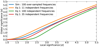
Figure 5: Relation to estimate the number of oversampled frequencies $P$ needed in equation 2 to compute the trial factor. “Eq 1” denotes the results of applying the equation 1 for a specific number of independent frequencies.

We select the $P$ to correct the local significance $\geq 4\sigma$ to correct precisely the results of the high-significance candidates. Figure 5 shows that adopting $P=35$ gives the best agreement with the over-sampled analysis for the relationship between the global significance and the local significance. Consequently, we choose $P=35$ for this work, resulting in a trials factor of 12,285 ($351$$\times$$35$). The resulting global significances for the high local significances are:

1. $\approx$3.5$\sigma$ for a “local significance” of $5.5\sigma$

2. $\approx$2.8$\sigma$ for “local significance” of $\approx$5$\sigma$

3. $\approx$1.8$\sigma$ for a “local significance” of $\approx$4.5$\sigma$

4. $<$1$\sigma$ for “local significance” $<$4.5$\sigma$.

4.5 Significance correction

We also perform a correction to the significances listed in Table 2, focusing only on the high-significance candidates. Artificial LCs are generated from each of these candidates using the approach by Emmanoulopoulos, (2013). Next, we calculate the frequency of $X\sigma$ events detected for these artificial LCs in the periodicity searches. We then calculate a “calibrated” significance based on the determined frequency of $X\sigma$ events.

The methods are the LSP, the GLSP, the REDFIT, PDM, CWT, and the DFT. We simulated $10^{6}$ LCs for the LSP, GLSP, CWT, and DFT methods. For the PDM and REDFIT methods, we only simulated $2\times 10^{5}$ LCs due to computational constraints. The results are shown in Table 5. The methods with the largest corrections are LSP, GLSP, and PDM, while the blazars with the largest corrections are PG 1553+113 and PKS 2155$-$304.

Another correction in the significance is implemented by generating artificial LCs based on a power-law approach by using the technique presented by Timmer and Koenig, (1995). The generated artificial LCs have the same flux distribution, standard deviation, and median flux as the original LCs. To perform this correction, we use the slopes and their uncertainties of Table 4. Specifically, we consider three different slope values: slope minus uncertainty, slope, slope plus uncertainty. The results are shown in Table 6. The methods with the largest corrections are GLSP and PDM, while the blazars with the largest corrections are OJ 014 and PG 1553+113.

4.6 Flux distribution

The analysis of the flux distribution of blazars can provide clues about the physical origin of the observed variability (e.g.,  Uttley et al.,, 2005). This analysis is performed using the PDF of the flux distribution. The PDFs are then fitted with normal and lognormal distributions (e.g.,  Bhatta and Dhital,, 2020). A normal flux distribution would indicate that emission is generated by the linear addition of independent components (an additive process; Biteau and Giebels,, 2012). Whereas, the multiplication of independent components produces a lognormal distribution as a reaction chain (a multiplicative process; Uttley et al.,, 2005).

To evaluate these two PDF functional forms, we employ two different methods. The Shapiro-Wilk test is the most sensitive at rejecting the null hypothesis of a normal distribution (Shapiro and Wilk,, 1965). We reject the null hypothesis if p$<$0.05. The other method employed is the maximum likelihood estimation (MLE). The MLE analysis is performed by fitdistrplus. Finally, to discriminate between both PDF fits, we use the AIC.

The results are listed in Table 4. Both the Shapiro-Wilk and MLE tests show that the lognormal PDF is a better representation of the flux distributions for most of the blazars in our sample (Shah et al.,, 2018). However, for S5 0716+71, the normal distribution is preferred (see Figure 6). The preference for a normal distribution over a lognormal one appears to be rare in the overall blazar population.

As mentioned previously, the flux distribution can be interpreted as reflecting the physics of the jet and the accretion disk. In one scenario discussed by Rieger, (2019) and references therein, a lognormal $\gamma$-ray flux distribution is associated with fluctuations in the accretion disk at different radii, which propagate inward to produce an aggregate multiplicative effect in the innermost disk. This disturbance is then transmitted to the jet (Shah et al.,, 2018). In contrast, an additive process is appropriate to model the combined emission from many uncorrelated regions in the jet. Many models of this sort have been proposed and can produce skewed normal distributions (see e.g. Biteau and Giebels,, 2012, and references therein).

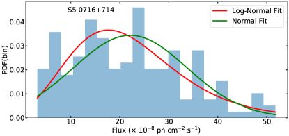
Figure 6: Fits of the S5 0716+714 $\gamma$-ray flux distribution for both normal and lognormal PDFs. The Shapiro-Wilk and MLE tests indicate that the normal PDF fits the LC best.

4.7 Evaluation of methods against noise

We now evaluate the periodicity detection methods when periodicity is present but the oscillating fluxes are contaminated by noise (VanderPlas,, 2018). These methods are LSP, GLSP, REDFIT, PDM, CWT, and DFT. We consider four different noises: “white noise”, “pink noise” (generating random power-law indices in the range [$0.8-1.2$]), “red noise” (with power-law indices in the range [$1.8-2.2$]) and “broken power-law” models.

To implement this scenario, we define a sinusoidal function

$$\phi(t)=O+A\sin\bigg{(}\frac{2\pi t}{T}+\theta\bigg{)},$$ (4)

where the parameters are the offset ($O$), the amplitude ($A$), the period ($T$), and the phase ($\theta$). The offset, amplitude, and phase are randomly selected from the values obtained for each of the 24 candidates from the Markov Chain Monte Carlo sinusoidal fitting method from P20. We also evaluate any bias in the detection by defining a periodicity range based on the ones from our sample (that is, $[1.5-4.5]$ years). From here, we check if a period is more likely to be detected than others.

We simulate 100,000 sinusoidal LCs for each period-noise combination. Both pink and red noise LCs are produced by applying the Python package colorednoise, which is based on Timmer and Koenig, (1995). The noisy LCs from broken power-law models are generated by the Python package of Conolly, (2015), which is derived from Emmanoulopoulos, (2013).

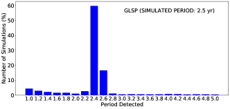
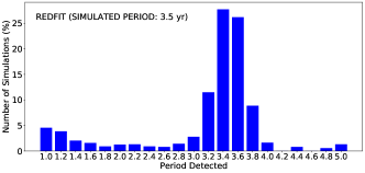
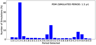
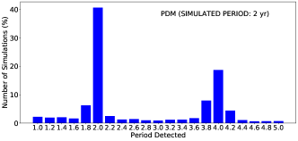
Figure 7: Results of the evaluation of the false-positive detection rates for the various periodicity-detection methods. Top: The results for the GLSP and REDFIT methods in the case of a sinusoidal LC with periods of 2.5 yrs (left) and 3.5 yrs (right) that is contaminated with red noise. These results indicate that these methods are robust for periodicity detection against red noise. Bottom: The results of the PDM simulations for periods of 1.5 yrs (left) and 2 yrs (right) contaminated with red noise. The harmonic effects observed by P20 are also shown.

The results from the different methods depend strongly on the noise pattern. The worst results are obtained for white noise and the broken power-law model, with average detection rates of 5%-20%. The method that is the most sensitive to noise is DCF, having the lowest detection rate for all noise patterns. The methods are most robust for fluxes that are contaminated with red noise. In particular, the methods that perform the best are CWT, GLSP and REDFIT, with detection rates of $\approx$25%-65% (see Figure 7). Any bias in detecting a specific period is not observed. However, there is a tendency for detection to be more sensitive to noise when the periods are on the higher end of our range, i.e., [3.5-4.5] yr. This is actually expected since fewer cycles would be included in the data. The exception is pink noise, which results in roughly constant detection rates for all the periods for each method (detection rates $\approx$12%-17%). Finally, the PDM simulations show the harmonic effects that were observed in P20. Harmonic effects are only observed when the sinusoidal LCs are contaminated by red noise (see Figure 7).

4.8 Lower energy counterparts

For some of the blazars in our sample, $\sim$year-long periods have previously been reported at lower energies. In this section, we review an incomplete segment of the relevant literature, primarily focusing on PG 1553+113 and PKS 2155$-$304, which arguably are the most popular and promising candidates. Covino et al., (2020) also summarize studies that have reported periodic LCs for PG 1553+113 and PKS 2155$-$304 in $\gamma$-ray and optical bands. Another recent discussion on the optical emission of PKS 2155$-$304 and S5 0716+714 (another high-significance periodicity source) can be found at the end of section 3.3.1 of Bhatta and Dhital, (2020).

Ackermann et al., (2015) first identified a $\approx 2.1\,\mathrm{yr}$ periodicity in the optical, radio, and $\gamma$-ray bands for PG 1553+113. Their $2.1\,\mathrm{yr}$ period agrees with our results. A later study by Covino et al., (2020) used Gaussian process modeling and a longer temporal baseline to search for periodicity in PG 1553+113. This study found that the quality of the fit in both the optical and $\gamma$-ray bands can be improved by including a component with a similar period to the one found in our results ($\approx 2.2\,\mathrm{yr}$).

To our knowledge, the first positive identification of $\sim$year-long periods for PKS 2155$-$304 was found in the optical band by Fan et al., (2000). The periods they reported were approximately $4.2\,\mathrm{yrs}$ and $7\,\mathrm{yrs}$. A later study by Zhang et al., (2014) used a much longer temporal baseline for analyzing optical data, but did not recover these multi-year periods as primary periodicities. Instead, Zhang et al., (2014) reported a period of $\approx 0.87\,\mathrm{yrs}$, and suggested that the $4.2\,\mathrm{yr}$ and $7\,\mathrm{yr}$ periods reported by Fan et al., (2000) may be respectively 4th and 7th harmonics of the primary $0.87\,\mathrm{yr}$ period. The optical periodicity of $\approx 0.87\,\mathrm{yrs}$ for PKS 2155$-$304 is approximately half of the $\gamma$-ray periodicity of $\approx 1.7\,\mathrm{yrs}$ that we report in this work. Sandrinelli et al., (2014) also reported a detection of the $\approx 0.87\,\mathrm{yr}$ periodicity in the optical band, as well as a tentative detection of a $\sim$year-long periodicity (similar to the $\approx 1.7\,\mathrm{yrs}$ periodicity in $\gamma$-rays that we report here). Their findings were reiterated in Sandrinelli et al., (2016). There is some indication of the $0.87\,\mathrm{yr}$ period in Figure 2 of the publication by Covino et al., (2020), but that period was not the focus of their work. Covino et al., (2020) explain the seemingly discrepant periodicity measurements for PKS 2155$-$304 as possibly arising from differences in the noise models considered in the data analysis.

There are indications from some studies of consistent periodicities in the optical and $\gamma$-ray bands. For example, a recent analysis by Bhatta, (2021) found similar periods in the optical and $\gamma$-ray bands for two of our high-significance sources: $\approx 1.7\,\mathrm{yrs}$ for PKS 2155$-$304 and $\approx 2.7\,\mathrm{yrs}$ for S5 0716+714. In particular, they did not find evidence for the $0.87\,\mathrm{yr}$ optical period for PKS 2155$-$304 reported in Zhang et al., (2014). They argued that consistent periods in different bands is evidence of the periodicity being genuine.

5 Periodicity Interpretation

A variety of scenarios have been proposed in the literature to explain periodic emission in blazars. Possible interpretations of long-term periodicity can be grouped into two categories: (1) periodicity in single black hole systems, and (2) periodicity in binary black hole systems.

5.1 Periodicity in single black hole systems

In the first category, the emission mechanism is interpreted in the context of a single-SMBH system, where the periodic emission is produced by modulations in the accretion flow or by jet precession. For example, Mohan and Mangalam, (2015) propose a scenario in which plasma inhomogeneities from the accretion disk propagate into the jet and generate periodic emission due to helical motions along magnetic surfaces within the jet. In models proposed in Villata and Raiteri, (1999) and Ostorero et al., (2004), precession of the jet axis induces periodic variation in the line-of-sight emission.

Alternatively, periodicity could emerge from overall modulation of the accretion power, which is (sensibly) assumed to be reflected in the jet power. Gracia et al., (2003) invoked such scenario for the periodicity of PKS 2155$-$304 (see H.E.S.S Collaboration,, 2016). The lognormal shape of the flux PDF suggests an underlying multiplicative process (see $\S$4.6); as such, it favors an accretion-disk origin for the periodicity over an additive process such as jets-in-jet (e.g., Uttley et al.,, 2005; Rieger,, 2019). Since accretion disks in the vicinity of SMBHs are expected to be dominated by radiation pressure, they are subject to a variety of instabilities (Lightman and Eardley,, 1974), which can lead to limit-cycle behavior that conceivably appears as quasi-periodic emission over a few cycles (Frank et al.,, 2002). Recent 3-dimensional simulations of a single SMBH give a concrete example of opacity-driven light curve variability lasting for $2-6$ cycles, encompassing a span of years to decades (Jiang et al.,, 2020). Over a few cycles, such variability may appear to be quasi-periodic.

5.2 Periodicity in binary black hole systems

The second category of proposed mechanisms invokes an SMBHB. There are two variations of this scenario: (i) perturbations caused by the secondary SMBH destabilize the accretion flow of the primary SMBH, modulating the accretion rate and, as a consequence, the luminosity of the blazar (Sandrinelli et al.,, 2016); (ii) the periodic emission may be due to jet precession, ultimately caused by the orbiting SMBHs (Sobacchi et al.,, 2017). The SMBHB hypothesis has been applied to explain the LC of PG 1553+113 (e.g., Cavaliere et al.,, 2017; Sobacchi et al.,, 2017; Tavani et al.,, 2018).

Major galaxy mergers are found more frequently at a moderate redshift of about $z\sim 1$ when galaxies are also more gas-rich (e.g., Tacconi,, 2010; Koss et al.,, 2018). In turn, the number of SMBHBs should increase with increasing redshift and increasing mass (Volonteri et al.,, 2009). Most of our candidates reside at redshifts $z\gtrsim 1$ (see Table 1).

In order to discriminate between different hypotheses, the periodicity search may be complemented by spectroscopy. Two different approaches can be useful to infer the presence of an SMBHB by using optical emission lines: radial velocity shifts and line shapes. Regarding radial velocity shifts, the lines are expected to oscillate about their rest-frame wavelength on the time scale corresponding to the orbital period (e.g., Liu et al.,, 2014, typically one targets the $\rm{H\beta}$ and $\rm{Mg{II}}$ lines). The other technique to infer close binary systems is to observe double-peaked profiles in the emission lines (e.g. H$\beta$, Kovačević et al.,, 2020).

5.3 Application of the binary hypothesis to PG 1553+113 and PKS 2155$-$304

Here we discuss the application of the binary hypothesis to two blazars in our sample with the highest-significance periodicity: PG 1553+113 and PKS 2155$-$304. These candidates are arguably the most promising because they are bright and have the greatest number of cycles ($\approx 6$ for PG 1553+113, $\approx 7$ for PKS 2155$-$304), and our autoregression analysis (ARFIMA/ARIMA) reports compatible periods with the methods of Table 3.

Covino et al., (2020) used Gaussian processes to analyze data from optical and previous Fermi-LAT observations. They found that adding a periodic component increased the statistical quality of fit for both candidates PG 1553+113 and PKS 2155$-$304 (although it is less convincing for PG 1553+113). The large number of cycles also helps in addressing the concerns raised by Vaughan et al., (2016) regarding spurious periodicity in LCs with only a few putative periods present. Also note that the significance we report has increased with the addition of 3 years of data; in contrast, adding new data for quasar PG 1302$-$102 resulted in a decrease in significance for the periodicity, which was seen as evidence against the authenticity of the periodicity (Liu et al.,, 2018). The idea was that if the periodicity were genuine, one would generally expect the significance of the detected period to become larger with new data. We note that the latest upper bound on the binary fraction of blazars from the Pulsar Timing Array (at most $\approx 1/1000$ blazars host binaries with orbital periods less than 5 years, Holgado et. al,, 2018) is compatible with the presence of few true SMBHBs in the Fermi-LAT catalog (Holgado et. al,, 2018).

For PKS 2155$-$304, there is a disparity in the mass estimates for the SMBH. The $M_{\rm BH}-L_{\rm bulge}$ relation suggests a central black hole mass of $M_{\rm BH}\gtrsim 2\times 10^{8}M_{\odot}$. On the other hand, VHE variability on time scales of $\lesssim$ 200 seconds suggest a black hole mass of $M_{\rm BH}\lesssim 4\times 10^{7}M_{\odot}$ (Rieger,, 2010). Variability in the X-ray band supports a lower mass estimate (Hayashida et al.,, 1998; Czerny et al.,, 2001). Rieger, (2010) argued that the discrepancy in mass estimates could be explained if PKS 2155$-$304 hosts a SMBHB: the $M_{\rm BH}-L_{\rm bulge}$ relation measures the binary mass while the fast variability reflects the mass of the secondary SMBH. This scenario requires that the jet emission comes mostly from the secondary SMBH, which is prima facie consistent with recent simulations of accreting unequal-mass binaries (Duffell et al.,, 2020). These simulations show that the secondary can accrete as much as $10\times$ faster than the primary. The different mass estimates constitute a bound on the SMBHB mass ratio$-q$ $\lesssim 0.2$, which implies that the secondary accretes at $\approx 3-10\times$ the rate of the primary (as seen in the simulations of Duffell et al.,, 2020). However, the physics of jet launching is rather complicated and not fully understood, so caution is warranted with circumstantial evidence such as this. Caution is also warranted when applying 2-dimensional thin-disk simulation results such as from Duffell et al., (2020), since that setup uses a variety of approximations. We refer to Rieger, (2019) and references therein for a recent overview of the binary hypothesis for PKS 2155$-$304. Attempts to explain the short time-scale variability without a binary are given in Begelman et al., (2008) and Levinson, (2007).

For PG 1553+113, variability on a 2400-second time scale leads to an SMBH mass estimate of $M_{\rm BH}\approx 4\times 10^{7}$ - $8\times 10^{8}M_{\odot}$, depending on the black hole’s spin (with higher spins implying larger masses, Dhiman et al.,, 2021). However, an estimate based on the $M_{\rm BH}$$-$$L_{\rm bulge}$ relation is not possible because the host galaxy has not yet been identified. As a basis for discussion, let us consider the orbital parameters from the binary model proposed by Cavaliere et al., (2017): primary SMBH mass $5\times 10^{8}M_{\odot}$, mass ratio $q=0.1$, eccentricity $e\approx 0.2$. In the model, mild non-zero eccentricity is required for the secondary SMBH to perturb the presumed jet from the primary SMBH on the orbital time scale. Thin-disk simulations find two values of the eccentricity that are stable under gas-driven binary evolution, $e=0$ (circular) and $e\approx 0.45$ (Zrake et al.,, 2021; D’Orazio et al.,, 2021). Thus, one may infer that the $e=0.2$ binary has been circularizing for some time due to gravitational wave emission. Consistency then requires that the evolution of the binary is already dominated by the emission of gravitational waves (i.e., the orbital radius is less than the “gas decoupling” orbital radius). Let the binary semi-major axis be $a$ and its total mass be $M$. We can estimate the orbital period when gas-driven evolution is on par with gravitational wave-driven evolution by assuming post-Newtonian orbital evolution (Peters,, 1964) and using $d\log a/d\log M=-l$. $l$ is the “accretion eigenvalue”, which determines the rate at which the binary semi-major axis evolves (and whether the binary is expanding or shrinking). Here, $l\sim\mathcal{O}(1)$ is determined by gas-accretion physics from thin-disk simulations. In following this procedure, we can set $a$, the rate of gas-driven evolution, to that of the gravitational-wave—driven evolution and solve for the orbital period. A positive value of $l$ corresponds to a gas-driven inspiral, which is reasonable for large disk Mach numbers ($\gtrsim 25$; Tiede et al.,, 2020) typically expected in AGN disks. Let us consider an accretion rate equal to the Eddington limit (assuming a typical efficiency of $\epsilon=0.1$). Even if we use a very large value $l=10$ (which results in a shorter orbital period at decoupling), we find that the orbital period at decoupling is nearly 6 years. Thus, under these standard assumptions, the proposed binary seems to have transitioned into the gravitational wave-driven regime with an orbital period of $\approx 1.5$ years (in the source frame). It would be interesting to carefully compute the orbital evolution history to see whether the proposed eccentricity of $e=0.2$ at the current orbital separation is consistent with the equilibrium value prior to the time of decoupling.

Lastly, simulations of accreting binaries have generally shown two possible main periodicities in accretion rates$-$that of the binary’s orbital period, $T_{\rm binary}$, and that of an overdensity (called a “lump”) orbiting at larger radii with a period $\approx(5-10)\times T_{\rm binary}$. The lump period is expected to dominate for mass ratios $q\gtrsim 0.2$ (Duffell et al.,, 2020; Farris et al.,, 2014; D’Orazio et al.,, 2013) and eccentricities $e\lesssim 0.1$ (Miranda, et al., 2017; Zrake et al.,, 2021). If the periodic LCs revealed in this study correspond to the lump period in a circumbinary disk, then the SMBHBs are orbiting faster and are thus closer to merging. Future measurements of gravitational waves from SMBHBs could reveal whether the electromagnetic emission is being modulated by the lump or the binary orbital period (D’Orazio et al.,, 2015).

6 Summary

In this work, we analyze the $\gamma$-ray LCs of the most promising 24 periodicity candidates presented by P20. Relative to P20, these LCs are extended from 9 to 12 years of Fermi-LAT data, the energies are expanded from $>$1 GeV to $>$0.1 GeV, increasing the signal-to-noise ratio. In addition, the upper limits are treated in a way that allows us to retain information about the flux variations. We also employ an improved version of our periodicity-search pipeline, composed of ten different statistical methods to infer periods and three associated techniques to get the significance. This pipeline is improved by including the ARIMA/ARFIMA autoregresive algorithm. As a result, we have obtained a sample with periodic $\gamma$-ray emission detected at global significance $\gtrsim 3\sigma$. This sample consists of five blazars$-$ four BL Lacs, S5 0716+714, OJ 014, PG 1553+113, and PKS 2155$-$304, and one FSRQ, PKS 0454$-$234.

Table 1: Comparison of periods and local significance for the blazars analyzed in P20. The significance and periods reported here are the average of those obtained in the different methods employed in the the periodicity-search analysis (to allow a comparison with P20). From top to the bottom: 5$\sigma$ candidates, and low significance candidates. The 5$\sigma$ candidates are sorted according to the number of algorithms that yielded a 5 $\sigma$ detection (see Table 2). The low-significance candidates are sorted according to the median of their significance (excluding the REDFIT since it gives a maximum significance of 2.5$\sigma$). Note that this median significance does not have an actual statistical meaning; it is used as an arbitrary way that combines all significance to sort the candidates. The blazars are characterized by their Fermi-LAT 4FGL source name, equatorial coordinates (deg), AGN type, redshift, association name, period (in years), and significance obtained by Peñil et al., (2020), and finally, the last column lists the average period (in years) and significance obtained in this work. Note that some sources have two significant periods (organized by the peak amplitude), denoted by $\star$.

4FGL Source Name	RA(J2000)	Dec(J2000)	Type	Redshift	Association Name	P20 Period (S/N)	Period (S/N)
						[yr]	[yr]
J1555.7+1111	238.93169	11.18768	bll	0.433	PG 1553+113	2.2 ($>$4.0$\sigma$)	2.2 ($>$5.0$\sigma$)
J0811.3+0146	122.86418	1.77344	bll	1.148	OJ 014	4.3 ($>$3.5$\sigma$)	4.1 (5.0$\sigma$)
J2158.8$-$3013	329.71409	$-$30.22556	bll	0.116	PKS 2155$-$304	1.7 ($>$3.0$\sigma$)	1.7 (5.0$\sigma$)
J0457.0$-$2324	74.26096	$-$23.41384	fsrq	1.003	PKS 0454$-$234	2.6 ($>$2.5$\sigma$)	3.6 (5.0$\sigma$)
J0721.9+7120$\star$	110.48882	71.34127	bll	0.127	S5 0716+714	2.8 ($>$2.5$\sigma$) 0.9 ($>$2$\sigma$)	2.7 (5.0$\sigma$) 0.9 (2.5$\sigma$)
J0428.6$-$3756	67.17261	$-$37.94081	bll	1.11	PKS 0426$-$380	3.4 (3.0$\sigma$)	3.6 (4.5$\sigma$)
J0449.4$-$4350	72.36042	$-$43.83719	bll	0.205	PKS 0447$-$439	2.5 (3.0$\sigma$)	1.9 ($>$4.0$\sigma$)
J2258.0$-$2759$\star$	344.50485	$-$27.97588	fsrq	0.926	PKS 2255$-$282	1.3 ($>$3.5$\sigma$)	2.8 (4.0$\sigma$) 1.4 (3.0$\sigma$)
J0043.8+3425	10.96782	34.42687	fsrq	0.966	GB6 J0043+3426	1.8 (4.0$\sigma$)	1.9 (4.0$\sigma$)
J0252.8$-$2218	43.20377	$-$22.32386	fsrq	1.419	PKS 0250$-$225	1.2 ($>$2.5$\sigma$)	1.2 (4.0$\sigma$)
J1248.2+5820$\star$	192.07728	58.34622	bll	–	PG 1246+586	2.0 (3.0$\sigma$)	2.1 (4.0$\sigma$) 1.4 (3.0$\sigma$)
J1146.8+3958	176.73987	39.96861	fsrq	1.089	S4 1144+40	3.3 ($>3.0$$\sigma$)	3.3 ($>$3.5$\sigma$)
J0818.2+4223	124.56174	42.38367	bll	0.530	S4 0814+42	2.2 (3.5$\sigma$)	2.2 (3.5$\sigma$)
J0521.7+2113	80.44379	21.21369	bll	0.108	TXS 0518+211	2.8 ($>$3.0$\sigma$)	3.1 ($>$3.0$\sigma$)
J1903.2+5541	285.80851	55.67557	bll	–	TXS 1902+556	3.8 ($>$2.5$\sigma$)	3.3 ($>$3.0$\sigma$)
J0303.4$-$2407	45.86259	$-$24.12074	bll	0.266	PKS 0301$-$243	2.0 (3.0$\sigma$)	2.1 (3.0$\sigma$)
J2056.2$-$4714$\star$	314.06768	$-$47.23386	fsrq	1.489	PKS 2052$-$47	1.7 ($>$2.5$\sigma$)	3.1 (2.5$\sigma$) 1.7 (3.0$\sigma$)
J1454.5+5124	223.63225	51.413868	bll	–	TXS 1452+516	2.1 ($>$3.5$\sigma$)	2.1 (2.5$\sigma$)
J1303.0+2435	195.75454	24.56873	bll	0.993	MG2 J130304+2434	2.0 ($>$2.5$\sigma$)	2.1 (2.5$\sigma$)
J0102.8+5825	15.71134	58.41576	fsrq	0.644	TXS 0059+581	2.1 (3.0$\sigma$)	4.0 ($>$2.0$\sigma$)
J1649.4+5238	252.35208	52.58336	bll	–	87GB 164812.2+524023	2.7 ($>$2.5$\sigma$)	2.8 ($>$2.0$\sigma$)
J0211.2+1051	32.81532	10.85811	bll	0.2	MG1 J021114+1051	1.7 ($>$3.5$\sigma$)	2.9 ($>$2.0$\sigma$)
J0501.2$-$0157	75.30886	$-$1.98359	fsrq	2.291	S3 0458$-$02	1.7 ($>$2.5$\sigma$)	3.8 (2.0$\sigma$)
J0210.7$-$5101	32.68952	$-$51.01695	fsrq	1.003	PKS 0208$-$512	2.6 ($>$3.0$\sigma$)	3.8 (1.5$\sigma$)

Table 2: List of time periods and uncertainties (top) with their associated significance (bottom) for the periodic-emission candidates following a similar structure as Table 1. Note that there are some sources with two periods with high significance (organized by the amplitude of the peak), which are denoted by $\star$. The symbol $\dagger$ denotes the PDM results that present the harmonic effect described in Peñil et al., (2020). The symbol $\ddagger$ denotes periods that were presented in the CWT for 12 years of LC data (see Figure 1). Furthermore, note that the REDFIT method only gives a maximum of significance of $2.5\sigma$ (see P20 for details). All periods are in years.

Association	LSP	GLSP	LSP	REDFIT	PDM	CWT	DFT-Welch
Name	Power-Law	Boostrap	Simulated LC
PG 1553+113	$2.1^{\pm 0.2}_{5.4\sigma}$	$2.1^{\pm 0.2}_{5.6\sigma}$	$2.2^{\pm 0.2}_{5.4\sigma}$	$2.1^{\pm 0.2}_{>2.5\sigma}$	$2.2^{\pm 0.1}_{5.1\sigma}$	$\ddagger 2.2^{\pm 0.4}_{5.3\sigma}$	$2.3^{\pm 0.3}_{5.1\sigma}$
OJ 014	$4.2^{\pm 0.5}_{2.5\sigma}$	$4.1^{\pm 0.4}_{5.0\sigma}$	$4.2^{\pm 0.4}_{5.3\sigma}$	$4.2^{\pm 1.1}_{>2.5\sigma}$	$4.1^{\pm 0.1}_{5.1\sigma}$	$\ddagger 4.4^{\pm 0.9}_{5.3\sigma}$	$3.9^{\pm 1.2}_{4.1\sigma}$
PKS 2155$-$304	$1.7^{\pm 0.1}_{4.1\sigma}$	$1.7^{\pm 0.1}_{5.2\sigma}$	$1.7^{\pm 0.1}_{5.0\sigma}$	$1.7^{\pm 0.1}_{>2.5\sigma}$	$\dagger 3.4^{\pm 0.2}_{5.0\sigma}$	$\ddagger 1.7^{\pm 0.3}_{3.1\sigma}$	$1.8^{\pm 0.1}_{5.0\sigma}$
PKS 0454$-$234	$3.6^{\pm 0.2}_{2.8\sigma}$	$3.5^{\pm 0.4}_{5.3\sigma}$	$3.5^{\pm 0.4}_{5.0\sigma}$	$3.5^{\pm 0.3}_{2.5\sigma}$	$3.5^{\pm 0.4}_{5.1\sigma}$	$\ddagger 3.9^{\pm 0.8}_{4.9\sigma}$	$3.7^{\pm 0.2}_{3.2\sigma}$
S5 0716+714$\star$	$2.7^{\pm 0.4}_{4.0\sigma}$ $0.9^{\pm 0.1}_{3.0\sigma}$	$2.6^{\pm 0.4}_{5.3\sigma}$	$2.6^{\pm 0.3}_{5.2\sigma}$	$2.7^{\pm 0.4}_{>2.5\sigma}$	$2.9^{\pm 0.3}_{5.0\sigma}$	$\ddagger 2.9^{\pm 0.8}_{5.1\sigma}$ $0.9^{\pm 0.1}_{2.5\sigma}$	$2.7^{\pm 0.5}_{3.1\sigma}$
PKS 0426$-$380	$3.5^{\pm 0.6}_{2.8\sigma}$	$3.6^{\pm 0.5}_{5.3\sigma}$	$3.5^{\pm 0.6}_{5.2\sigma}$	$3.5^{\pm 0.4}_{2.0\sigma}$	$3.4^{\pm 0.5}_{4.8\sigma}$	$\ddagger 3.6^{\pm 0.5}_{4.2\sigma}$	$3.9^{\pm 0.4}_{2.1\sigma}$
PKS 0447$-$439	$1.9^{\pm 0.2}_{2.3\sigma}$	$1.8^{\pm 0.2}_{4.4\sigma}$	$1.9^{\pm 0.2}_{5.0\sigma}$	$1.9^{\pm 0.2}_{2.1\sigma}$	$\dagger 4.0^{\pm 0.4}_{4.2\sigma}$	$2.0^{\pm 0.5}_{4.8\sigma}$	$1.9^{\pm 0.2}_{4.1\sigma}$
PKS 2255$-$282$\star$	$1.4^{\pm 0.1}_{2.7\sigma}$ $2.8^{\pm 0.3}_{1.9\sigma}$	$2.8^{\pm 0.4}_{4.3\sigma}$ $1.4^{\pm 0.1}_{3.0\sigma}$	$2.8^{\pm 0.3}_{4.1\sigma}$ $1.4^{\pm 0.1}_{4.0\sigma}$	$2.8^{\pm 0.3}_{1.5\sigma}$ $1.4^{\pm 0.1}_{1.5\sigma}$	$2.7^{\pm 0.2}_{5.0\sigma}$	$\ddagger 3.1^{\pm 0.3}_{4.8\sigma}$ $1.4^{\pm 0.3}_{2.9\sigma}$	$3.1^{\pm 0.9}_{3.5\sigma}$
GB6 J0043+3426	$1.9^{\pm 0.2}_{3.7\sigma}$	$1.9^{\pm 0.4}_{4.0\sigma}$	$1.9^{\pm 0.2}_{5.2\sigma}$	$1.9^{\pm 0.2}_{2.5\sigma}$	$\dagger 3.9^{\pm 0.2}_{3.9\sigma}$	$2.0^{\pm 0.5}_{4.1\sigma}$	$2.0^{\pm 0.2}_{4.0\sigma}$
PKS 0250$-$225	$1.2^{\pm 0.2}_{3.8\sigma}$	$1.2^{\pm 0.1}_{4.7\sigma}$	$1.2^{\pm 0.1}_{2.7\sigma}$	$1.2^{\pm 0.1}_{>2.5\sigma}$	$\dagger 2.4^{\pm 0.1}_{4.0\sigma}$	$1.2^{\pm 0.2}_{4.4\sigma}$	$1.4^{\pm 0.1}_{1.9\sigma}$
PG 1246+586$\star$	$2.1^{\pm 0.2}_{4.0\sigma}$ $1.4^{\pm 0.1}_{4.1\sigma}$	$2.2^{\pm 0.1}_{4.9\sigma}$	$2.2^{\pm 0.2}_{5.1\sigma}$ $1.4^{\pm 0.2}_{4.8\sigma}$	$2.1^{\pm 0.2}_{>2.5\sigma}$ $1.4^{\pm 0.1}_{2.2\sigma}$	$\dagger 4.2^{\pm 0.1}_{4.0\sigma}$	$\ddagger 2.2^{\pm 0.3}_{3.9\sigma}$	$2.4^{\pm 0.4}_{2.6\sigma}$
S4 1144+40	$3.3^{\pm 0.2}_{3\sigma}$	$3.5^{\pm 0.5}_{5.1\sigma}$	$3.3^{\pm 0.6}_{3.7\sigma}$	$3.3^{\pm 0.6}_{2.5\sigma}$	$3.2^{\pm 0.5}_{5.0\sigma}$	$\ddagger 3.4^{\pm 0.9}_{4.1\sigma}$	$3.5^{\pm 0.1}_{2.9\sigma}$
S4 0814+42	$2.2^{\pm 0.2}_{3.0\sigma}$	$2.2^{\pm 0.2}_{4.6\sigma}$	$2.3^{\pm 0.1}_{4.2\sigma}$	$2.2^{\pm 0.2}_{1.9\sigma}$	$2.2^{\pm 0.3}_{3.0\sigma}$	$\ddagger 2.3^{\pm 0.3}_{4.0\sigma}$	$1.9^{\pm 0.1}_{2.2\sigma}$
TXS 0518+211	$3.0^{\pm 0.4}_{2.9\sigma}$	$3.1^{\pm 0.4}_{5.4\sigma}$	$3.2^{\pm 0.4}_{2.9\sigma}$	$3.1^{\pm 0.4}_{2.5\sigma}$	$3.1^{\pm 0.2}_{5.0\sigma}$	$\ddagger 3.2^{\pm 0.5}_{3.3\sigma}$	$3.2^{\pm 0.4}_{4.0\sigma}$
TXS 1902+556	$3.3^{\pm 0.4}_{2.7\sigma}$	$3.3^{\pm 0.3}_{4.8\sigma}$	$3.3^{\pm 0.3}_{3.8\sigma}$	$3.3^{\pm 0.4}_{>2.5\sigma}$	$3.3^{\pm 0.3}_{4.7\sigma}$	$\ddagger 3.4^{\pm 0.7}_{3.0\sigma}$	$3.3^{\pm 0.6}_{2.4\sigma}$
PKS 0301$-$243	$2.1^{\pm 0.2}_{3.0\sigma}$	$2.1^{\pm 0.2}_{4.4\sigma}$	$2.1^{\pm 0.2}_{3.2\sigma}$	$2.1^{\pm 0.2}_{2.2\sigma}$	$\dagger 4.0^{\pm 0.1}_{5.0\sigma}$	$2.1^{\pm 0.1}_{3.2\sigma}$	$2.0^{\pm 0.4}_{1.9\sigma}$
PKS 2052$-$47$\star$	$1.6^{\pm 0.2}_{3.0\sigma}$	$3.1^{\pm 0.3}_{3.8\sigma}$ $1.7^{\pm 0.2}_{3.1\sigma}$	$1.7^{\pm 0.1}_{4.8\sigma}$ $3.0^{\pm 0.3}_{4.1\sigma}$	$1.6^{\pm 0.1}_{2.2\sigma}$	$3.3^{\pm 0.3}_{2.3\sigma}$	$1.7^{\pm 0.3}_{2.2\sigma}$	$3.3^{\pm 0.3}_{2.4\sigma}$
TXS 1452+516	$2.0^{\pm 0.4}_{2.6\sigma}$	$2.0^{\pm 0.2}_{2.5\sigma}$	$2.0^{\pm 0.3}_{2.9\sigma}$	$2.2^{\pm 0.4}_{1.9\sigma}$	$2.0^{\pm 0.1}_{2.3\sigma}$	$2.1^{\pm 0.6}_{3.0\sigma}$	$1.8^{\pm 0.2}_{2.3\sigma}$
MG2 J130304+2434	$2.0^{\pm 0.2}_{2.5\sigma}$	$2.0^{\pm 0.1}_{1.5\sigma}$	$2.0^{\pm 0.2}_{3.9\sigma}$	$2.0^{\pm 0.2}_{2.4\sigma}$	$\dagger 4.0^{\pm 0.1}_{5.0\sigma}$	$2.2^{\pm 0.4}_{4.1\sigma}$	$2.2^{\pm 0.2}_{1.0\sigma}$
TXS 0059+581	$4.0^{\pm 0.6}_{2.3\sigma}$	$1.2^{\pm 0.1}_{1.3\sigma}$	$4.0^{\pm 0.6}_{2.4\sigma}$	$4.0^{\pm 0.7}_{1.2\sigma}$	$4.2^{\pm 0.1}_{5.0\sigma}$	$\ddagger 4.6^{\pm 0.7}_{2.0\sigma}$	$4.0^{\pm 0.2}_{4.1\sigma}$
87GB 164812.2+524	$2.8^{\pm 0.9}_{2.7\sigma}$	$2.7^{\pm 0.2}_{1.1\sigma}$	$2.8^{\pm 0.3}_{1.6\sigma}$	$2.8^{\pm 0.4}_{2.4\sigma}$	$3.0^{\pm 0.1}_{4.4\sigma}$	$3.3^{\pm 0.4}_{2.0\sigma}$	$3.3^{\pm 0.5}_{3.2\sigma}$
MG1 J021114+1051	$2.8^{\pm 0.3}_{2.6\sigma}$	$2.9^{\pm 0.6}_{2.0\sigma}$	$2.8^{\pm 0.3}_{2.4\sigma}$	$2.8^{\pm 0.3}_{1.6\sigma}$	$2.8^{\pm 0.2}_{4.0\sigma}$	$\ddagger 3.1^{\pm 0.7}_{2.2\sigma}$	$3.0^{\pm 1.0}_{2.0\sigma}$
S3 0458$-$02	$3.7^{\pm 0.9}_{1.8\sigma}$	$3.7^{\pm 0.6}_{1.2\sigma}$	$3.7^{\pm 0.6}_{1.9\sigma}$	$3.7^{\pm 0.6}_{1.7\sigma}$	$3.8^{\pm 0.3}_{3.0\sigma}$	$4.4^{\pm 0.7}_{2.1\sigma}$	$4.0^{\pm 0.3}_{3.0\sigma}$
PKS 0208$-$512	$3.8^{\pm 0.5}_{1.3\sigma}$	$3.7^{\pm 0.4}_{2.0\sigma}$	$3.9^{\pm 0.6}_{0.8\sigma}$	$3.8^{\pm 0.6}_{0.7\sigma}$	$3.8^{\pm 0.5}_{2.5\sigma}$	$\ddagger 4.4^{\pm 0.4}_{2.8\sigma}$	$5.4^{\pm 0.6}_{4.1\sigma}$

Table 3: List of periods provided by the Markov Chain Monte Carlo sine fits and the Bayesian quasi-periodic oscillation methods following a similar structure as Table 1. Additionally, the maximum sensitivity of the Bayesian quasi-periodic oscillation analysis is included (see P20 for more details). Xs in the Bayesian and Sensitivity columns indicate that the algorithm did not converge in the frequency range considered and thus no value was reported. The # in ARFIMA/ARIMA column indicates that the model used is ARIMA due to the LC being non-stationary (resulting from augmented Dickey-Fuller test, see $\S$3.2). The period obtained with the ACF from the residuals generated from the original LC and the ARIMA/ARFIMA model is also listed. Note that there are some sources with two periods (organized by the significance), which are denoted by $\star$. Finally, Xs in the Dickey-Fuller and Box-Ljung columns indicate that the null hypothesis is rejected in such tests ($\S$3.2). All periods are in years.

Association Name	MCMC Sine Fitting	Bayesian	Sensitivity	ARFIMA/ARIMA	ACF Residuals	Dickey-Fuller	Box-Ljung
PG 1553+113$\star$	2.1 $\pm$ 0.1	2.1	5.2%	[17, 0.449, 18]	2.8 (2.0$\sigma$) 2.0 (1.5$\sigma$)	✓	✓
OJ 014	4.4 $\pm$ 0.1	3.9	8.1%	[19, 0.471, 15]	3.8 (1.6$\sigma$)	✓	✓
PKS 2155$-$304$\star$	1.7 $\pm$ 0.1	1.7	10%	[10, 0.435, 10]	1.6 (2.1$\sigma$) 1 (1.6$\sigma$)	✓	✓
PKS 0454$-$234$\star$	3.5 $\pm$ 0.1	X	X	[20, 0.493, 20]	2.0 (2.0$\sigma$) 1.2 (1.6$\sigma$)	✓	✓
S5 0716+714	2.7 $\pm$ 0.1	3.2	13.6%	[12, 0.447, 14]	1.2 (1.6$\sigma$)	✓	✓
PKS 0426$-$380$\star$	3.2 $\pm$ 0.1	3.2	22.5%	[14, 0.47, 14]	3.4 (2.3$\sigma$) 2.2 (1.9$\sigma$)	✓	✓
PKS 0447$-$439$\star$	$1.8^{+0.1}_{-0.6}$	2.1	8.2%	[15, 0.45, 14]	1.5 (2.2$\sigma$) 2.5 (1.5$\sigma$)	✓	✓
PKS 2255$-$282	3.1 $\pm$ 0.1	2.1	20.6%	[18, 0.441, 19]	2.8 (1.6$\sigma$)	✓	✓
GB6 J0043+3426	1.8 $\pm$ 0.1	2.1	7.5%	[9, 0.472, 10]	2.0 (2.1$\sigma$)	✓	✓
PKS 0250$-$225	1.2 $\pm$ 0.1	3.3	8.2%	#[5, 1, 8]	1.3 (1.5$\sigma$)	X	✓
PG 1246+586	2.2 $\pm$ 0.1	2.8	3.6%	[16, 0.436, 20]	3.5 (2.8$\sigma$)	✓	✓
S4 1144+40	3.5 $\pm$ 0.1	3.4	35.1%	[18, 0.433, 19]	2.5 (2.0$\sigma$)	✓	✓
S4 0814+42	2.1 $\pm$ 0.1	X	X	[14, 0.451, 14]	3.1 (2.2$\sigma$)	✓	✓
TXS 0518+211	$3.1^{+0.1}_{-0.8}$	3.2	10.2%	[15, 0.333, 13]	2.9 (1.9$\sigma$)	✓	✓
TXS 1902+556	3.3 $\pm$ 0.1	3.4	7.7%	[20, 0.41, 15]	3.4 (1.6$\sigma$)	✓	✓
PKS 0301$-$243	$1.4^{+0.8}_{-0.1}$	2.1	11.1%	[17, 0.451, 20]	1 (1.7$\sigma$)	✓	✓
PKS 2052$-$47	2.6 $\pm$ 0.1	3.0	15.1%	[18, 0.441, 19]	1.6 (1.9$\sigma$)	✓	✓
TXS 1452+516	2.1 $\pm$ 0.1	2.0	8.8%	[19, 0.448, 18]	1.7 (1.9$\sigma$)	✓	✓
MG2 J130304+2434	1.2 $\pm$ 0.1	X	X	[19, 0.471, 20]	2.0 (2.1$\sigma$)	✓	✓
TXS 0059+581	4.1 $\pm$ 0.1	3.5	9.5%	[16, 0.391, 18]	3.9 (1.4$\sigma$)	✓	✓
87GB 164812.2+524023	$2.9^{+0.8}_{-0.1}$	3.1	18.4%	[18, 0.445, 20]	2.0 (1.2$\sigma$)	✓	✓
MG1 J021114+1051	1.7 $\pm$ 0.1	1.5	11.3%	[15, 0.414, 14]	2.6 (1.95$\sigma$)	✓	✓
S3 0458$-$02$\star$	1.5 $\pm$ 0.2	3.2	15.3%	[10, 0.453, 8]	3.8 (2.2$\sigma$) 2.1 (2.0$\sigma$)	✓	X
PKS 0208$-$512	$4.0^{+0.5}_{-1.0}$	X	X	#[2, 1, 8]	1.2 (1.0$\sigma$)	X	X

Table 4: List of power-spectrum indices inferred from the PSRESP method with their uncertainties and success fractions. Also listed are the results of the Shapiro-Wilk (with associated $p$ values) and MLE (with the differences in AIC between both PDF fittings provided as percentages) tests. The Shapiro-Wilk and MLE columns also indicate whether the flux distribution is better fitted with a normal or a lognormal functional form.

Association Name	Power Spectral Index	Success Fraction (%)	Shapiro-Wilk	MLE
PG 1553+113	1.2$\pm$0.4	87.2	Log-normal (1.1$\times$10-2)	Log-normal (5.1%)
OJ 014	1.2$\pm$0.4	53.1	Log-normal (4.1$\times$10-2)	Log-normal (1.6%)
PKS 2155$-$304	1.0$\pm$0.6	75.2	Log-normal (3.0$\times$10-4)	Log-normal (6.4%)
PKS 0454$-$234	1.3$\pm$0.3	50.4	Log-normal (9.2$\times$10-3)	Log-normal (3.1%)
S5 0716+714	1.1$\pm$0.3	23.9	Normal (2.1$\times$10-2)	Normal (2.2%)
PKS 0426$-$380	1.3$\pm$0.4	72.1	Log-normal (2.0$\times$10-2)	Log-normal (5.8%)
PKS 0447$-$439	1.3$\pm$0.3	53.4	Log-normal (3.0$\times$10-3)	Log-normal (6.7%)
PKS 2255$-$282	1.3$\pm$0.5	87.4	Log-normal (1.6$\times$10-5)	Log-normal (13.9%)
GB6 J0043+3426	0.8$\pm$0.5	87.7	Log-normal (8.5$\times$10-6)	Log-normal (7%)
PKS 0250$-$225	1.2$\pm$0.4	55.4	Log-normal (1.2$\times$10-5)	Log-normal (13.7%)
PG 1246+586	0.9$\pm$0.3	17.3	Log-normal (7.5$\times$10-3)	Log-normal (2.9%)
S4 1144+40	1.2$\pm$0.4	88.0	Log-normal (8.8$\times$10-4)	Log-normal (9.2%)
S4 0814+42	1.3$\pm$0.3	47.1	Log-normal (2.4$\times$10-2)	Log-normal (3.2%)
TXS 0518+211	1.3$\pm$0.4	74.5	Log-normal (1$\times$10-3)	Log-normal (8.6%)
TXS 1902+556	1.1$\pm$0.4	91.8	Log-normal (1.2$\times$10-3)	Log-normal (5.2%)
PKS 0301$-$243	1.1$\pm$0.4	82.4	Log-normal (9.0$\times$10-7)	Log-normal (21.6%)
PKS 2052$-$47	1.2$\pm$0.3	37.0	Log-normal (8.0$\times$10-5)	Log-normal (8.7%)
TXS 1452+516	1.2$\pm$0.3	51.8	Log-normal (2.0$\times$10-4)	Log-normal (12.3%)
MG2 J130304+2434	1.1$\pm$0.5	86.1	Log-normal (8.5$\times$10-5)	Log-normal (18.5%)
TXS 0059+581	1.3$\pm$0.3	61.3	Log-normal (6.5$\times$10-5)	Log-normal (13.5%)
87GB 164812.2+524023	1.3$\pm$0.4	97.2	Log-normal (5$\times$10-3)	Log-normal (11.2%)
MG1 J021114+1051	1.2$\pm$0.3	18.1	Log-normal (5.6$\times$10-4)	Log-normal (6.2%)
S3 0458$-$02	1.2$\pm$0.4	68.2	Log-normal (1.4$\times$10-4)	Log-normal (10.1%)
PKS 0208$-$512	1.6$\pm$0.4	59.3	Log-normal (4.9$\times$10-6)	Log-normal (14.3%)

Table 5: Results of the correction to the significance based on the approach by Emmanoulopoulos, (2013). The corrections are listed in pairs with the significance inferred from the pipeline provided to the left of the arrow and the corrected significance provided to the right.

Association Name	LSP	GLSP	REDFIT	PDM	CWT	DFT-Welch
PG 1553+113	5.4$\sigma\rightarrow$4.6$\sigma$	5.6$\sigma\rightarrow$4.2$\sigma$	2.5$\sigma\rightarrow$2.4$\sigma$	5.1$\sigma\rightarrow$4.1$\sigma$	5.3$\sigma\rightarrow$4.0$\sigma$	5.1$\sigma\rightarrow$4.0$\sigma$
OJ 014	5.3$\sigma\rightarrow$4.1$\sigma$	5.0$\sigma\rightarrow$4.4$\sigma$	2.5$\sigma\rightarrow$2.3$\sigma$	5.1$\sigma\rightarrow$4.3$\sigma$	5.3$\sigma\rightarrow$4.8$\sigma$	4.1$\sigma\rightarrow$3.8$\sigma$
PKS 2155$-$304	5.0$\sigma\rightarrow$4.1$\sigma$	5.2$\sigma\rightarrow$4.5$\sigma$	2.5$\sigma\rightarrow$1.8$\sigma$	5.0$\sigma\rightarrow$3.9$\sigma$	3.1$\sigma\rightarrow$2.5$\sigma$	5.0$\sigma\rightarrow$4.1$\sigma$
PKS 0454$-$234	5.0$\sigma\rightarrow$4.3$\sigma$	5.3$\sigma\rightarrow$4.5$\sigma$	2.5$\sigma\rightarrow$2.3$\sigma$	5.1$\sigma\rightarrow$4.5$\sigma$	4.9$\sigma\rightarrow$4.0$\sigma$	3.2$\sigma\rightarrow$2.3$\sigma$
S5 0716+714	5.2$\sigma\rightarrow$4.7$\sigma$	5.3$\sigma\rightarrow$4.8$\sigma$	2.5$\sigma\rightarrow$2.3$\sigma$	5.0$\sigma\rightarrow$4.5$\sigma$	5.1$\sigma\rightarrow$4.4$\sigma$	3.1$\sigma\rightarrow$2.4$\sigma$

Table 6: Results of the correction to the significance using the power-law approach and the slopes and uncertainties provided in 4. Three different slopes are studied: $\beta_{min}$, $\beta$, $\beta_{max}$. The corrections are shown in pairs with the significance inferred from the pipeline provided to the left of the arrow and the corrected significance proved to the right.

Association Name	Slope	LSP	GLSP	REDFIT	PDM	CWT	DFT-Welch
PG 1553+113	$\beta_{min}$=0.8 $\beta$=1.2 $\beta_{max}$=1.6	5.4$\sigma\rightarrow$4.8$\sigma$ 5.4$\sigma\rightarrow$4.8$\sigma$ 5.4$\sigma\rightarrow$4.3$\sigma$	5.6$\sigma\rightarrow$4.6$\sigma$ 5.6$\sigma\rightarrow$4.8$\sigma$ 5.6$\sigma\rightarrow$4.4$\sigma$	2.5$\sigma\rightarrow$2.0$\sigma$ 2.5$\sigma\rightarrow$2.0$\sigma$ 2.5$\sigma\rightarrow$2.1$\sigma$	5.1$\sigma\rightarrow$4.4$\sigma$ 5.1$\sigma\rightarrow$4.1$\sigma$ 5.1$\sigma\rightarrow$4.0$\sigma$	5.3$\sigma\rightarrow$4.8$\sigma$ 5.3$\sigma\rightarrow$4.7$\sigma$ 5.3$\sigma\rightarrow$4.2$\sigma$	5.1$\sigma\rightarrow$4.2$\sigma$ 5.1$\sigma\rightarrow$4.1$\sigma$ 5.1$\sigma\rightarrow$4.4$\sigma$
OJ 014	$\beta_{min}$=0.8 $\beta$=1.2 $\beta_{max}$=1.6	5.3$\sigma\rightarrow$4.6$\sigma$ 5.3$\sigma\rightarrow$4.1$\sigma$ 5.3$\sigma\rightarrow$4.7$\sigma$	5.0$\sigma\rightarrow$4.2$\sigma$ 5.0$\sigma\rightarrow$3.9$\sigma$ 5.0$\sigma\rightarrow$3.9$\sigma$	2.5$\sigma\rightarrow$1.9$\sigma$ 2.5$\sigma\rightarrow$2.1$\sigma$ 2.5$\sigma\rightarrow$2.1$\sigma$	5.1$\sigma\rightarrow$4.1$\sigma$ 5.1$\sigma\rightarrow$4.0$\sigma$ 5.1$\sigma\rightarrow$4.2$\sigma$	5.2$\sigma\rightarrow$4.7$\sigma$ 5.2$\sigma\rightarrow$4.2$\sigma$ 5.2$\sigma\rightarrow$4.2$\sigma$	4.1$\sigma\rightarrow$3.9$\sigma$ 4.1$\sigma\rightarrow$3.7$\sigma$ 4.1$\sigma\rightarrow$3.7$\sigma$
PKS 2155$-$304	$\beta_{min}$=0.4 $\beta$=1.0 $\beta_{max}$=1.6	5.0$\sigma\rightarrow$4.0$\sigma$ 5.0$\sigma\rightarrow$4.3$\sigma$ 5.0$\sigma\rightarrow$4.3$\sigma$	5.2$\sigma\rightarrow$3.9$\sigma$ 5.2$\sigma\rightarrow$4.6$\sigma$ 5.2$\sigma\rightarrow$4.3$\sigma$	2.5$\sigma\rightarrow$1.9$\sigma$ 2.5$\sigma\rightarrow$1.9$\sigma$ 2.5$\sigma\rightarrow$1.8$\sigma$	5.0$\sigma\rightarrow$4.1$\sigma$ 5.0$\sigma\rightarrow$4.3$\sigma$ 5.0$\sigma\rightarrow$4.1$\sigma$	3.1$\sigma\rightarrow$2.9$\sigma$ 3.1$\sigma\rightarrow$2.9$\sigma$ 3.1$\sigma\rightarrow$2.9$\sigma$	5.0$\sigma\rightarrow$4.2$\sigma$ 5.0$\sigma\rightarrow$4.0$\sigma$ 5.0$\sigma\rightarrow$4.4$\sigma$
PKS 0454$-$234	$\beta_{min}$=1.0 $\beta$=1.3 $\beta_{max}$=1.6	5.0$\sigma\rightarrow$4.6$\sigma$ 5.0$\sigma\rightarrow$4.7$\sigma$ 5.0$\sigma\rightarrow$4.4$\sigma$	5.3$\sigma\rightarrow$4.1$\sigma$ 5.3$\sigma\rightarrow$4.3$\sigma$ 5.3$\sigma\rightarrow$4.2$\sigma$	2.5$\sigma\rightarrow$2.3$\sigma$ 2.5$\sigma\rightarrow$2.1$\sigma$ 2.5$\sigma\rightarrow$2.1$\sigma$	5.1$\sigma\rightarrow$3.9$\sigma$ 5.1$\sigma\rightarrow$4.1$\sigma$ 5.1$\sigma\rightarrow$4.3$\sigma$	4.9$\sigma\rightarrow$3.7$\sigma$ 4.9$\sigma\rightarrow$3.7$\sigma$ 4.9$\sigma\rightarrow$3.9$\sigma$	3.2$\sigma\rightarrow$2.8$\sigma$ 3.2$\sigma\rightarrow$2.8$\sigma$ 3.2$\sigma\rightarrow$2.9$\sigma$
S5 0716+714	$\beta_{min}$=0.8 $\beta$=1.1 $\beta_{max}$=1.4	5.2$\sigma\rightarrow$4.5$\sigma$ 5.2$\sigma\rightarrow$4.8$\sigma$ 5.2$\sigma\rightarrow$4.2$\sigma$	5.3$\sigma\rightarrow$4.1$\sigma$ 5.3$\sigma\rightarrow$4.5$\sigma$ 5.3$\sigma\rightarrow$4.7$\sigma$	2.5$\sigma\rightarrow$2.0$\sigma$ 2.5$\sigma\rightarrow$2.1$\sigma$ 2.5$\sigma\rightarrow$2.1$\sigma$	5.0$\sigma\rightarrow$4.1$\sigma$ 5.0$\sigma\rightarrow$4.2$\sigma$ 5.0$\sigma\rightarrow$4.6$\sigma$	5.1$\sigma\rightarrow$4.3$\sigma$ 5.1$\sigma\rightarrow$4.6$\sigma$ 5.1$\sigma\rightarrow$4.2$\sigma$	3.1$\sigma\rightarrow$2.7$\sigma$ 3.1$\sigma\rightarrow$2.7$\sigma$ 3.1$\sigma\rightarrow$2.8$\sigma$

Table 7: Results of evaluating the chance of detecting spurious periodic fluxes with different noise scenarios.

Analysis Method	Type of Noise	Significance	Number of LCs [%]
LSP	White Noise	$<$1.0$\sigma$ 1.0$\sigma$ 2.0$\sigma$	95.7 2.2 2.1
	Pink Noise	$<$1.0$\sigma$ 1.0$\sigma$ 2.0$\sigma$	81.2 8.6 10.2
	Red Noise	$<$1.0$\sigma$ 1.0$\sigma$ 2.0$\sigma$	58.4 27.1 14.5
	Broken P-L	$<$1.0$\sigma$ 1.0$\sigma$	99.1 0.9
GLSP	White Noise	$<$1.0$\sigma$	100
	Pink Noise	$<$1.0$\sigma$ 1.0$\sigma$	99.3 0.7
	Red Noise	$<$1.0$\sigma$ 1.0$\sigma$	99.1 0.9
	Broken P-L	$<$1.0$\sigma$ 1.0$\sigma$	99.1 0.9
REDFIT	White Noise	$<$1.0$\sigma$ 1.0$\sigma$	99 1
	Pink Noise	$<$1.0$\sigma$ 1.0$\sigma$ 2.0$\sigma$	93.8 3.1 2.9
	Red Noise	$<$1.0$\sigma$ 1.0$\sigma$ 2.0$\sigma$	85.1 10.2 4.7
	Broken P-L	$<$1.0$\sigma$ 1.0$\sigma$	98.8 1.2
PDM	White Noise	$<$1.0$\sigma$ 1.0$\sigma$ 2.0$\sigma$	95.3 2.3 2.4
	Pink Noise	$<$1.0$\sigma$ 1.0$\sigma$ 2.0$\sigma$ 3.0$\sigma$	91.3 2.1 5.4 1.2
	Red Noise	$<$1.0$\sigma$ 1.0$\sigma$ 2.0$\sigma$	91.8 6.5 1.7
	Broken P-L	$<$1.0$\sigma$ 1.0$\sigma$	97.8 2.2
CWT	White Noise	$<$1.0$\sigma$	100
	Pink Noise	$<$1.0$\sigma$ 1.0$\sigma$	99.1 0.9
	Red Noise	$<$1.0$\sigma$ 1.0$\sigma$	99.1 0.9
	Broken P-L	$<$1.0$\sigma$	100
DFT	White Noise	$<$1.0$\sigma$	100
	Pink Noise	$<$1.0$\sigma$ 1.0$\sigma$ 2.0$\sigma$	98.3 1.1 0.6
	Red Noise	$<$1.0$\sigma$ 1.0$\sigma$ 2.0$\sigma$	98.5 0.8 0.7
	Broken P-L	$<$1.0$\sigma$ 1.0$\sigma$	98.9 1.1

This section reports the LCs of the low-significance blazars.

References

- Abdo et al., (2010) Abdo, A.A., Ackermann, M., Ajello, M., et al. 2010, ApJ, 722, 1
- Abdollahi et al., (2020) Abdollahi, S., Acero, F., Ackermann, M., et al. 2020, ApJS, 247, 1
- Abdollahi et al., (2022) Abdollahi, S., Acero, F., Baldini, L., et al. 2020, ApJS, 260, 2
- Ackermann et al., (2015) Ackermann, M., Ajello, M., Albert, A., et al. 2015, ApJ, 813, L41
- Ait Benkhali et al., (2020) Ait Benkhali, F., Hofmann, W., Rieger, F. M., et al., 2020, A&A, 634, A120
- Akaike, (1973) Akaike, H. 1973, Biometrika, 60, 255
- Astropy Collaboration, (2013) Astropy Collaboration, 2013, A&A, 558, A33
- Astropy Collaboration, (2018) Astropy Collaboration, 2018, ApJ, 156, 123
- Atwood et al., (2009) Atwood, W. B, Abdo, A. A., Ackermann, M., et al. 2009, ApJ, 697, 1071
- Ballet et al., (2020) Ballet, J., Burnett, T.H., Digel, S.W., et al., 2020, arXiv:2005.11208
- Atwood et al., (2013) Atwood, W., Albert, A., Baldini, L., et al. 2013, eConf C121028, 8, in Proc. 4th Fermi Symposium, Monterey
- Begelman et al., (1980) Begelman, M. C., Blandford, R.D., Rees, M.J., 1980, Nature, 287, 307
- Begelman et al., (2008) Begelman, M.C., Fabian, A.C., Rees, M. J., 2008, MNRAS, 384, 1
- Bhatta and Dhital, (2020) Bhatta, G., and Dhital, N. 2020, ApJ, 891, 120
- Bhatta, (2021) Bhatta, G., 2021, ApJ, 923, 1
- Bhatta, (2022) Bhatta, G., 2022, arXiv:2204.08923
- Biteau and Giebels, (2012) Biteau, J., and Giebels, B., 2012, A&A, 548, A123
- Bruel et al., (2018) Bruel, P., Burnett, T. H., Digel, S. W., et al., 2018, eprint arXiv:1810.11394
- Caceres, (2019) Caceres, G. A., Feigelson, E. D., Babu, G. J., et al. 2019, ApJ, 158, 21
- Cavaliere and Padovani, (1989) Cavaliere A., Padovani P. 1989, ApJ, 340, L5
- Cavaliere et al., (2017) Cavaliere, A., Tavani, M., and Vittorini, V. 2017, ApJ, 836, 220
- Chakraborty and Rieger, (2020) Chakraborty, N., Rieger, F. M. Rieger, 2020, arXiv:2010.01038.
- Chatfield, (2003) Chatfield, C. 2003, The Analysis of Time Series: An Introduction (6th ed.; New York: Chapman and Hall)
- Colpie, (2014) Colpi, M. 2014, SSRv, 183, 189
- Conolly, (2015) Connolly S., 2015, arXiv:1503.06676
- Covino et al., (2019) Covino, S., Sandrinelli, A., and Treves, A. 2019, MNRAS, 482, 1270
- Covino et al., (2020) Covino, S., Landoni, M., Sandrinelli, A., et al. 2020, ApJ, 895, 122
- Cumming et al., (1999) Cumming, A., Marcy, G. W., Butler, R. P. 1999, ApJ, 526, 890
- Czerny et al., (2001) Czerny, B., Nikołajuk, M., Piasecki, M., et al. 2001, MNRAS, 325, 2, 865-874
- Czerny et al., (2004) Czerny, B., 2004, astro-ph/0409254.
- Czesla et al., (2019) Czesla, S. 2019
- Delignette-Muller and Dutang, (2015) Delignette-Muller, M. L., and Dutang, C. 2015, Journal of Statistical Software, 64, 4
- Dhiman et al., (2021) Dhiman, V., Gupta, A. C., Gaur, H., et al. 2021, MNRAS, 506, 1
- Dickey and Fuller, (1979) Dickey, D. A., and Fuller, W. A., 1979, Journal of the American Statistical Association, 74 (366a), 427–431.
- D’Orazio et al., (2013) D’Orazio, D.J., Haiman, Z., MacFadyen, A., 2013, MNRAS, 436, 4, 2997-3020
- D’Orazio et al., (2015) D’Orazio, D.J., Haiman, Z., Duffell, P., et al., 2015, MNRAS, 452, 3, 2540-2545
- D’Orazio et al., (2021) D’Orazio, D.J., Duffell, P.C., 2021, ApJ, 914, L21
- Dosopoulou and Antonini, (2017) Dosopoulou, F., and Antonini, F. 2017, ApJ, 840, 31
- Duffell et al., (2020) Duffell, P.C., D’Orazio, D., Derdzinski, A, et al. 2020, ApJ, 901, 1
- Emmanoulopoulos, (2013) Emmanoulopoulos, D., McHardy, I. M., Papadakis, I. E., 2013, MNRAS, 433, 907
- Enoki et al., (2004) Enoki, M., Inoue, K. T., Nagashima, M., et al., 2004, ApJ, 615, 1
- Fan et al., (2000) Fan, J. H., and Lin, R. G., 2000, A&A, 355, 880
- Farris et al., (2014) Farris, B.D., Duffell, P., MacFadyen, A. I., et al. 2014, ApJ, 783, 2
- Feigelson, (2018) Feigelson, E., Babu, G. J., Caceres, G. A., 2018, Frontiers in Physics, 6, 80
- Foreman-Mackey et al., (2018) Foreman-Mackey D., Hogg David W. , Lang D., Goodman J. 2012, PASP, 125, 306
- Foster, (1996) Foster G. 1996, ApJ, 112, 1709
- Frank et al., (2002) Frank, J., King, A., Raine, D.J. 2002, Accretion Power in Astrophysics: Third Edition
- Gao et al., (2003) Gao, J. B., Cao, Y., Lee, J.-M. 2003, Physics Letters A, 314, 392
- Goyal et al., (2017) Goyal, A., Stawarz, Ł., Ostrowski, M., et al. 2017, ApJ, 837, 127
- Goyal, (2018) Goyal, A., 2018, Galaxies, 6(1), 34
- Gracia et al., (2003) Gracia, J., Peitz, J., Keller, C., et al. 2003, MNRAS, 344, 2
- Gross and Vitells, (2010) Gross, E., and Vitells, O., 2010, The European Physical Journal C, 70, 1-2, 525-530
- Haiman et al., (2009) Haiman, Z., Kocsis, B., Menou, K., 2009, ApJ, 700, 2, 1952.
- Haring and Rix, (2004) Haring, N., and Rix, H.-W., 2004, ApJ, 604, L89
- Hayashida et al., (1998) Hayashida, K. et al., 1998, ApJ, 500, 2
- H.E.S.S Collaboration, (2016) H.E.S.S Collaboration, 2016, A&A, 598, A39
- Holgado et. al, (2018) Holgado, A. M., Sesana, A., Sandrinelli, A., Covino, et al. 2018, MNRAS, 481(1), L74-L78.
- Huppenkothen et al., (2013) Huppenkothen, D., et al. 2013, ApJ, 768, 13
- Ivezić et al., (2014) Ivezić Ž, Connolly, A.J. and Vanderplas, J.T. and Gray, A. 2014, Princeton University Press
- Jiang et al., (2012) Jiang, T., Hogg, D. W., and Blanton, M. R. 2012, ApJ, 759, 140
- Jiang et al., (2020) Jiang, Y-F., Blaes, O., 2020, ApJ, 900, 1
- Jolley et al., (2009) Jolley, E. J. D., Kuncic, Z., Bicknell, G. V., Wagner, S., 2009, MNRAS, 400, 3, 1521–1526.
- Kovačević et al., (2020) Kovačević, A.B., et al., 2020, A&A, 635, A1
- Koss et al., (2018) Koss, M.J., et al., 2018, Nature, 563, 7730
- Kunjaya et al., (2011) Kunjaya C., Mahasena P., Vierdayanti K., Herlie S., 2011, Astrophysics and Space Science, 336
- Kushwaha et al., (2017) Kushwaha, P., Sinha, A., Misra, R., et al., 2017, ApJ, 849, 2
- Levinson, (2007) Levinson, A., 2007, ApJ, 671, 1
- Li et al., (2018) Li, H. Z., Jiang, Y. G., Yi, T. F., et al. 2018, Ap&SS, 363, 3
- Lightman and Eardley, (1974) Lightman, A.P., and Eardley, D.M. 1974 ApJ, vol. 187, p.L1
- Lin et al., (2008) Lin, L., D.R. Patton, D.C. Koo, et al., 2008, ApJ, 681, 1
- Liu et al., (2014) Liu, X., Shen, Y., Bian, F., et al., 2014, ApJ, 789
- Liu et al., (2018) Liu, T., Gezari, S., Miller, M.C. 2018, ApJ, 859, 1
- Ljung and Box, (1978) Ljung, G. M. and Box, G. E. P. 1978, Biometrika, 65, 297
- Lomb, (1976) Lomb, N. R. 1976, Ap&SS, 39, 447
- Mattox, et al. (1996) Mattox J. R., Bertsch, D. L., Chiang, J., et al. 1996, ApJ, 461, 396
- Miranda, et al. (2017) Miranda, R., et al. 2017, MNRAS, 466, 1, 1170-1191
- Mohan and Mangalam, (2015) Mohan, P., Mangalam, A. 2015, ApJ, 805, 91
- Nakagawa and Masaki, (2013) Nakagawa, K., and Masaki, M., 2013, ApJ773, 177
- Ostorero et al., (2004) Ostorero, L., Villata, M., and Raiteri, C.M., 2004, A&A, 419, 913-925
- Peñil et al., (2020) Peñil, P. Dominguez, A., Buson, S., et al., 2020, ApJ, 896, 11
- Peters, (1964) Peters, P.C., 1964, Physical Review, 136, 4B, 1224-1232
- Prokhorov and Moraghan, (2017) Prokhorov D. A., and Moraghan A., 2017, MNRAS, 471, 3036
- Rieger, (2007) Rieger F. M., 2007, Ap&SS, 309, 271-275
- Rieger, (2010) Rieger F. M., Volpe, F., 2010, A&A, 520
- Rieger, (2019) Rieger F. M., 2019, Galaxies, 7, 1
- Sandrinelli et al., (2014) Sandrinelli A., Covino S., M., Treves A. 2014, ApJ, 793, 1
- Sandrinelli et al., (2016) Sandrinelli A., Covino S., Dotti M., Treves A. 2016, AJ, 151, 54
- Sandrinelli et al., (2017) Sandrinelli A., et al., 2017, A&A, 600, A132
- Scargle, (1981) Scargle, J. D. 1981, ApJS, 45, 1
- Scargle, (1982) Scargle, J. D. 1982, ApJ, 263, 835
- Schulz and Mudelsee, (2002) Schulz, M., and Mudelsee, M. 2002, Comput. Geosci., 28, 421
- Shah et al., (2018) Shah, Z., Mankuzhiyil, N., Sinha, A., et al., 2018, Research in Astronomy and Astrophysics, 18, 141
- Shapiro and Wilk, (1965) Shapiro, S. S., and Wilk, M. B. 1965, Biometrika, 52, 591
- Sobacchi et al., (2017) Sobacchi, E., Sormani, M. C., and Stamerra, A. 2017, MNRAS, 465, 161
- Sobolewska et al., (2014) Sobolewska, M. A., Siemiginowska, A., Kelly, B. C., et al., 2014, ApJ786, 143
- Soltan, (1982) Soltan, A. 1982, MNRAS, 200, 115
- Stellingwerf, (1978) Stellingwerf, R.F. 1978, ApJ, 224, 953
- Tacconi, (2010) Tacconi, L. J. et al., 2010, Nature, 2010, 463, 781
- Tarnopolski, (2020) Tarnopolski M., Żywucka N., Marchenko V., Pascual-Granado J., 2020, ApJS, 250, 1
- Tavani et al., (2018) Tavani M., Cavaliere A., Munar-Adrover P., Argan A., 2018, ApJ, 854, 11
- Tiede et al., (2020) Tiede, C., Zrake, J., MacFadyen, A., et al., 2020, ApJ, 2020, 900, 1
- Timmer and Koenig, (1995) Timmer, J., and Koenig, M., 1995, A&A, 300, 707
- Torrence and Compo, (1998) Torrence, C., and Compo, G. P. 1998, Bulletin of the American Meteorological Society, 79, 61
- Urry, (1996) Urry, C. M., 1996, in Miller H. R., Webb J. R., Noble J. C., eds, Astronomical Society of the Pacific Conference Series Vol. 110, Blazar Continuum Variability. p. 391 (arXiv:astroph/9609023)
- Urry, (2011) Urry, C. M., A&A, 2011, 32, Issue 1-2, pp. 139-145
- Uttley et al., (2002) Uttley, P., McHardy, I.M., and Papadakis, I.E., 2002, MNRAS, 332, 1
- Uttley et al., (2005) Uttley, P., McHardy, I.M., and Vaughan, S, 2005 MNRAS, 359, 1
- Valtonen et al., (2016) Valtonen, M. J., Zola, S., Ciprini, S., et al. 2016, ApJ, 819, L37
- VanderPlas, (2018) VanderPlas, J. T. 2018, ApJS, 236, 1
- Vaughan, (2005) Vaughan, S. 2005, A&A, 431, 391
- Vaughan et al., (2016) Vaughan, S., Uttley, P., Markowitz, A. G., et al. 2015, MNRAS, 461, 3, 3145-3152
- Villata and Raiteri, (1999) Villata, M., and Raiteri, C. M., 1999, A&A347
- Virtanen et al., (2020) Virtanen, P., Gommers, R., Oliphant, T., et al. 2020, Nature Methods, 17, 261-272
- Volonteri et al., (2009) Volonteri, M., Miller, J. M., Dotti, M., 2009, ApJ, 703, L86
- Welch, (1967) Welch, P.D. 1967, IEEE Trans., AU-15, 2, 70
- Witta, (2006) Witta P. J. 2006, arXiv:astro-ph/0603728
- Wood et al., (2017) Wood, M., Caputo, R., Charles, E., et al. 2017, PoS ICRC2017
- Xu, (2019) Xu, C., 2019, AJ157, 127
- Yang et al., (2021) Yang, S., Yan, D., Zhang, P., et al. 2021, ApJ, 907, 105
- Zechmeister and Kürster, (2009) Zechmeister, M., Kürster M. 2009, A&A, 496, 577
- Zhang et al., (2014) Zhang B.-K., Zhao B.-K., Wang C.-X., Dai B.-Z, 2014, A&A, 14, 8
- (122) Zhang P.-F., Yan D.-H., Liao N.-H., Zeng W., Wang J.-C., Cao L.-J. 2017, ApJ, 835, 5
- (123) Zhang P.-F., Yan D.-H., Liao N.-H., Zeng W., Wang J.-C., Cao L.-J., 2017, ApJ, 842, 10
- (124) Zhang P.-F., Yan D.-H., Zhou J.-N., Fan Y.-Z., Wang J.-C., Zhang L. 2017, ApJ, 845, 8
- Zhang et al., (2020) Zhang P.-F., Dai-Hai, Y., Zhou, J.-N, et al., 2020, ApJ, 891, 163
- Zrake et al., (2021) Zrake J., Tiede, C., MacFadyen, A., et al., 2021, ApJ, 909, 1