Orbital liquid in the orbital Hubbard model in dimensions
Abstract
We demonstrate that the three-dimensional orbital Hubbard model can be generalized to arbitrary dimension , and that the form of the result is determined uniquely by the requirements that (i) the two-fold degeneracy of the orbital be retained, and (ii) the cubic lattice be turned into a hypercubic lattice. While the local Coulomb interaction is invariant for each basis of orthogonal orbitals, the form of the kinetic energy depends on the orbital basis and takes the most symmetric form for the so-called complex-orbital basis. Characteristically, with respect to this basis, the model has two hopping channels, one that is orbital-flavor conserving, and a second one that is orbital-flavor non-conserving. We show that the noninteracting electronic structure consists of two nondegenerate bands of plane-wave real-orbital single-particle states for which the orbital depends on the wave vector. Due to the latter feature each band is unpolarized at any filling, and has a non-Gaussian density of states at . The orbital liquid state is obtained by filling these two bands up to the same Fermi energy. We investigate the orbital Hubbard model in the limit , treating the on-site Coulomb interaction within the Gutzwiller approximation, thus determining the correlation energy of the orbital liquid and the (disordered) para-orbital states. In perfect analogy with the case of the spin Hubbard model, the Gutzwiller approximation is demonstrated to be exact at for the orbital Hubbard model, because of the collapse of electron correlations to a single site. At half-filling (one electron per site on average, ) one finds a Brinkman-Rice type “metal-insulator” transition in the orbital liquid, which is analogous to the transition for a paramagnetic state in the spin model, but occurs at stronger Hubbard interaction due to the enhanced kinetic energy provided by the non-conserving hopping channel. We show that the orbital liquid is the ground state everywhere in the phase diagram except close to half-filling at sufficiently large , where ferro-orbital order with real orbitals occupied is favored. The latter feature is shown to be specific for , being of mathematical nature due to the exponential tails in the density of states.
I Introduction
Our understanding of electron correlations in solids stems to a considerable extent from the Hubbard model [1]. This describes electrons which propagate on a lattice and interact by an on-site Coulomb interaction when two electrons with opposite spins occupy the same site. At half-filling (one electron per site) it provides a picture of a metal-insulator transition due to electron localization and of magnetism caused by superexchange according to ideas going back to Anderson [2]. Away from half-filling it represents the competition between the kinetic energy of the electrons and the localizing effect of the Coulomb interaction. An important development regarding the Hubbard model was the discovery by Metzner and Vollhardt that in the limit of infinite dimension () only the on-site correlations survive [3, 4]. They thus proved that in this limit the Gutzwiller approximation to the variational ground state wave function [5, 6, 7] becomes exact [8], and that a similar property applies [9] to the resonating valence-bond (RVB) state [10]. It was then shown that the ground state phase diagram of the doped Hubbard model at includes ferromagnetic (FM) and antiferromagnetic (AF) order stabilized at large Coulomb interaction [11].
The orbital Hubbard model [12, 13, 14, 15, 16], discussed in the present paper, describes spinless fermions which propagate on a lattice of atoms with twofold degenerate orbitals and which interact by an on-site Coulomb interaction when two electrons occupy both orbitals on a site. Importantly, the hopping strength is dependent on the orientation of the orbitals with respect to the hopping direction. Obviously, with twofold orbital degeneracy replacing twofold spin degeneracy, the orbital model closely resembles the spin model, but there is a crucial difference: in the spin model the local symmetry is SU(2) but in the orbital model it is the threefold rotation group and moreover this is linked to the hopping. As an immediate consequence the model contains, in addition to the familiar orbital-conserving hopping channel (analogous to the spin-conserving hopping channel in the (spin) Hubbard model), also an orbital-flipping hopping channel. This leads in the 3D case to the existence of an orbital liquid (OL) state [12, 13], in analogy to a spin liquid [17, 18], which is disordered in a way different from paramagnetism. Our aim is to analyze the limit along the lines set out by Metzner and Vollhardt and explore whether this gives further insight into the properties of the orbital Hubbard model and the OL state in particular.
The orbital Hubbard model comes from the field of spin-orbital physics, which has developed over the last two decades into a very active and challenging part of solid state physics which unifies frustrated magnetism and the phenomena in strongly correlated electron systems. It arose from the pioneering ideas of Kugel and Khomskii [19] who recognized that in transition metal oxides with partly filled degenerate orbitals, both the spin and the orbital degrees of freedom are quantum variables and have to be treated on equal footing. At large local Coulomb interaction most of these compounds are Mott (or charge-transfer) insulators due to electron localization, and superexchange arises from coupled spins and orbitals together [20, 21, 22]. More recently similar phenomena have been found in ultracold fermion systems in optical lattices [23].
In the degenerate-orbital case [24], quantum fluctuations in the insulating state are enhanced with respect to the nondegenerate case [25, 26, 27]. In some cases these joint fluctuations could even trigger a new state of quantum matter—a spin-orbital liquid in model [28] or real systems [29, 30, 31]. In most cases, however, one finds spin-orbital order due to spin interactions of a Heisenberg form with SU(2) symmetry, coupled to anisotropic orbital superexchange [32, 33, 34, 35, 36, 37, 38, 39, 40, 41, 42, 43, 44, 45, 46, 47, 48, 49, 50, 51], in agreement with the Goodenough-Kanamori rules [52]. These interactions give in general entangled ground states [53, 54, 55, 56, 57, 58]. We remark that the physical properties of such systems are very rich and depend on whether the orbital degrees of freedom are of , , or type. The main difference is the spatial character of the orbitals which makes their interactions directional.
An issue of high interest is how such systems, characterized by the presence of orbital and spin degrees of freedom, behave under doping, i.e., how their properties compare with the more familiar behavior of doped spin systems, such as the high- cuprates [59, 60, 61]. In the latter systems remarkable progress has been achieved by employing dynamical mean-field theory (DMFT) [62], which gave very valuable insights into the transport properties [63] and spectral functions [64]. This theory, which is currently used widely for electronic structure calculations of strongly correlated materials where the one-electron description breaks down [65], is in fact based on the above-mentioned discovery by Metzner and Vollhardt regarding the Hubbard model [3, 4].
A realistic description of transition metal oxides with degenerate orbitals requires the treatment of spin-orbital physics in at least a degenerate Hubbard model, involving both orbital and spin degrees of freedom [22]. However, in particular situations the problem becomes somewhat simplified. In spin-orbital systems with FM order and weak spin-orbit coupling, the spins may be ignored because the spin flavor is conserved in the hopping processes, and the spins disentangle from the orbitals [66, 67] and do not contribute to the dynamics. The degenerate Hubbard model appropriate for the spin-orbital system [68] then reduces to an orbital Hubbard model with direction-dependent hopping.
When the active orbitals are of type this orbital Hubbard model is rather similar to the standard spin Hubbard model because the orbital flavor is then conserved in the hopping processes (like for spin) but the hopping is two-dimensional (2D) [29, 69]. This gives almost localized orbital polarons for single holes [70, 71] or orbital stripes due to self-organization of the doped Mott insulator [72, 73].
However, in doped FM systems with active orbitals [74, 75] the orbital flavor is not conserved, in contrast to the case above, and the kinetic energy consists of all possible hopping processes including those which change the orbital flavor. Obviously, this represents a qualitative difference with the spin Hubbard model. Moreover, it suggests that disordered phases are favored more in doped than in doped systems.
In doped manganites the FM metallic phase occurs due to the kinetic energy gain by the double exchange mechanism [76], because antiferromagnetic (AF) bonds hinder electron hopping while hopping is unrenormalized along FM bonds, and the electrons reorient the spins coupled to them by Hund’s rule exchange. Double exchange for strongly correlated electrons is indeed responsible for the spectacular properties of doped perovskite manganites [77, 78, 79], including colossal magnetoresistance in the FM metallic phase [80]. At low doping the -type AF order in La1-xSrxMnO3 favors electron transport within 2D planes, and gradually changes the spin order to FM along the axis. Increasing doping generates orbital polarons [81]. Already a single polaron triggers [82] an insulator-to-metal transition that occurs here to a FM metallic phase. Eventually, the orbitals decouple from the spins and a disordered orbital liquid (OL) phase arises in a 3D system [12, 13, 14, 15]. This OL phase may explain the cubic dispersion relation of magnons in the FM phase of some manganites which indicates that magnetic interactions are isotropic [83, 84] unless they couple strongly to orbital excitations [57]. Specifically this compound, La1-xSrxMnO3, provides a prime example of the physical situation represented by the orbital model studied in this paper, with the spins integrated out and the dynamics determined solely by the orbitals.
So the orbital Hubbard model, while still directly relevant for a class of doped FM insulators, is the simplest nontrivial multi-orbital model representing interacting lattice fermions, and as such presents an opportunity for studying fundamental issues in orbital dynamics. Moreover, because of their mathematical similarity one can readily compare its behavior with that of the (spin) Hubbard model, at the same time exploiting the wealth of results available for the latter one.
As stated, our overall aim is to investigate whether the limit of infinite dimension elucidates the characteristic features of the orbital Hubbard model, like it does for the spin Hubbard model [11]. In particular we want to establish which features found in the 3D case [12, 13, 14, 15] are characteristic for the model as such, i.e., continue to hold for arbitrary dimension up to , and which are specific for per se or are caused by the fact that at finite dimension the Gutzwiller approach is an approximation.
The purpose of this paper is therefore (i) to derive the orbital model at arbitrary dimension from the requirements that the twofold degeneracy of the orbitals be retained and that the cubic lattice symmetry be turned into a hypercubic symmetry; (ii) to highlight the fundamental difference with the spin Hubbard model which is that the orbital flavor is not conserved and the kinetic energy is therefore potentially larger, which should hinder orbital order and favor states with disordered orbitals; (iii) to demonstrate that the Gutzwiller approximation is again exact in the limit like it is for the (spin) Hubbard model, and next to investigate (iv) in what way the OL state avoids orbital polarization, and the role played therein by symmetry; (v) whether at half-filling electron localization induces a metal-insulator transition in the OL state and, if so, at which critical value of the on-site interaction (vi) what the nature is of the ground state (long-range order of ferro type or alternating type, or rather disordered of para-orbital type or orbital-liquid type), dependent on the strength of the interaction and the particle density .
The paper is organized as follows. In Sec. II.1 we introduce the orbital Hubbard model for spin-polarized electrons for a cubic lattice (), and discuss its symmetry properties. We show that the cubic symmetry of the hopping may be better appreciated when a particular basis consisting of two orbitals with complex coefficients is used. This serves to introduce the orbital model at general dimension and at in Sec. II.2. Next we use the translational invariance to present the noninteracting Hamiltonian in momentum space in Sec. II.3. Band dispersion and densities of states for complex and real single-particle states are presented in Secs. III.1 and III.2, respectively. In Sec. III.3 we address the single-particle eigenstates and show that they exhibit a generic splitting into a lower and an upper band. The orbital model is compared at dimension with the spin model in Sec. III.4 and we argue from the densities of states that its general feature is an enhanced kinetic energy. In Sec. III.5 we analyze the kinetic energy in dependence of filling and compare it for the simplest symmetry-broken states, disordered (para-orbital) states, and the OL state built from the single-particle eigenstates.
The electron correlations are described using the Gutzwiller approximation within a generalization of the Metzner approach [8, 9], analyzed in Sec. IV.1, and we evaluate the renormalized propagator at using the collapse of diagrams to a single site in Sec. IV.2. The general formalism for uniform and two-sublattice states is introduced in Sec. IV.3. In Sec. V we treat specific trial variational states: (i) ordered states in Sec. V.1, (ii) the OL phase in Sec. V.2, concluding the demonstration that the Metzner approach remains valid in the orbital case. In the next Section VI we compare the OL in the orbital Hubbard model with the paramagnet in the spin Hubbard model, and show that a Brinkman-Rice transition takes place in the OL just like in the paramagnet but for a considerably larger value of . The results of the numerical analysis and the phase diagram of the orbital Hubbard model at are presented in Sec. VII. At the end we focus on some general aspects of the orbital physics and suggest possible extensions of the present study (Sec. VIII.1). The paper is concluded in Sec. VIII.2 by pointing out the differences between the spin and orbital Hubbard model in infinite dimension. In the Appendix we present a proof that the orbital liquid phase is unpolarized.
II The orbital Hubbard model
II.1 The model at dimension
The usual choice of basis for orbitals in a 3D cubic lattice is to take
| (1) |
called real orbitals. However, because this basis is the natural one only for the bonds parallel to the axis but not for those in the plane, the kinetic energy takes then a rather nonsymmetric form, having a very different appearance depending on the bond direction. It is thus preferred to use instead the basis of complex orbitals at each site [85],
| (2) |
corresponding to “up” and “down” pseudospin flavors, with the local pseudospin operators defined as
| (3) |
For later reference it is convenient to introduce also electron creation operators which create electrons in orbital coherent states at site , defined as
| (4) |
in analogy with the well-known spin coherent states [86]. The local pseudospin operator in this state is
| (5) |
i.e., it behaves like a vector [87].
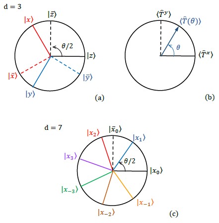
The parameter space of the coherent orbital (4) is a sphere, with the “poles” ( and ) corresponding to the complex orbitals and , and the “equator” () corresponding to (linear combinations of) the real orbitals,
| (6) |
The three real bases, , , and , associated with the cubic axes , , and , respectively, are obtained by setting the in-plane angle equal to , , and , for , and and to () for , as illustrated in Fig. 1(a).
In the complex-orbital representation the orbital Hubbard model for electrons in takes the form [13]
| (7) | |||||
where the parameter actually takes the value . This parameter is introduced here as a device by which one may interpolate between the standard 2-flavor Hubbard model with hopping at and the orbital model at . The appearance of the phase factors is characteristic for the orbital problem — they occur because the orbitals have an actual shape in real space so that each hopping process depends on the bond direction and on the orbitals between which hopping occurs. Moreover, Eq. (7) exhibits the crucial feature that (except at ) orbital flavor is not conserved, or, equivalently, that pseudospin is not conserved, compare Eq. (3).
The model (7) consists of the kinetic energy and the interorbital Coulomb interaction . The interaction is invariant under any local basis transformation to a pair of orthogonal orbitals, i.e., it gives an energy when a double occupancy occurs in any representation, i.e., either when both real orbitals are simultaneously occupied or when both complex orbitals are occupied,
| (8) |
We emphasize that this simple Hubbard-like form of the Coulomb interaction operator obtained here corresponds to the high-spin () charge excitations, , — these are the only excited states in a FM system. The parameter stands then for the onsite interorbital Coulomb repulsion, and is in fact lower than the intraorbital Coulomb element (Kanamori parameter) by due to Hund’s exchange in the triplet state, i.e., [33, 16].
Importantly, as noted in [13], the equivalence of the cubic axes shows up in the kinetic energy term in Eq. (7) in a transparent way, viz. as a formal invariance under threefold rotations of the phase angles in conjunction with a phase shift of the electron operators . So the relevant symmetry group is , with the doublets transforming as real representations, or equivalently the pairs transforming as conjugate complex representations.
II.2 Generalization to large dimension
This form, Eq. (7), therefore lends itself to a natural generalization of the orbital Hubbard model with two orbital flavors to large dimension as follows,
| (9) | |||||
with , where , and (i.e., taken odd for convenience but could also be even with only slightly different derivations below), and we note here that . So instead of three cubic axes we now have hypercubic axes , labelled by the index . Importantly, the number of orbital flavors remains two (as for spin ).
The real basis associated with axis is given by Eq. (6) with set equal to and to , respectively. This is illustrated in Fig. 1(c) for in comparison with the case for shown in Fig. 1(a). Figure 1(b) shows the associated behavior of the pseudospin vector, valid both for and for general .
The hopping parameter is scaled in the standard fashion [3, 8, 11] by in order that the average kinetic energy remains finite as becomes large. Below we will use the abbreviation whenever convenient. Again, the parameter takes the value for the orbital problem, in which the orbital flavor (pseudospin) is not conserved, while for the corresponding spin problem with hopping , in which the (spin) flavor is conserved. The interorbital Coulomb interaction is the same for any dimension as it stands for the on-site Coulomb repulsion when both orbital (or spin) flavors are occupied.
Obviously, the equivalence of the hypercubic axes manifests itself in the Hamiltonian as a -fold rotational symmetry, i.e., by being invariant under phase shifts of the electron operators in conjunction with shifts of the angles , in perfect analogy with the 3-fold rotational symmetry of . So is invariant under , with the doublets still transforming as real representations. In the limit the symmetry group turns into , which for practical purposes approaches continuous rotational symmetry U(1).
The generalization to dimension for the explicit form of the normalized real basis orbitals associated with the central axis in terms of the coordinates is obtained straightforwardly,
| (10) | |||||
| (11) |
of which Eq. (1) is seen to be the special case for . We observe that for general dimension , the “directional” orbital has a less pronounced directional shape than in the 3D case, because of the many finite contributions from all the coordinates with , although the square of the central coordinate still has the largest coefficient. The orthogonal orbital is perpendicular to the axis as in the 3D case (the coefficient of in is zero as ). When gets large the shape of resembles that of but with permuted coordinates (because Eq. (11) is obtained by replacing in Eq. (10) by ). Clearly, at each site all real-orbital basis sets are equivalent. We have made the arbitrary choice to use the set as the reference basis for real orbitals, and for convenience to drop the subscript .
II.3 Momentum space representation
Using translational invariance, we introduce creation and annihilation operators in momentum space,
| (12) |
where labels the orbital flavors, e.g. or , and is the number of sites. The free-electron part of , Eq. (9), describing the kinetic energy , may be represented upon Fourier transformation in the form
| (13) |
where the dispersion is given by orbital-conserving and orbital-non-conserving terms,
| (14) | |||||
| (15) |
It will turn out convenient to introduce the following definitions,
| (16) | |||||
| (17) | |||||
| (18) |
One may now absorb the phase factors from the offdiagonal elements of the matrix in Eq. (13) into the operators, by defining what we will call “phased” complex-orbital single-particle operators,
| (19) |
and rewrite as
| (20) |
If desired, the kinetic energy may also be rewritten from Eq. (13) in terms of the real-orbital operators,
where
| (22) | |||||
| (23) | |||||
| (24) |
The invariance with respect to the symmetry group of this real-orbital representation of is warranted by and both transforming as , and by and both transforming as real representations.
We note that whereas the kinetic-energy Hamiltonian (13), (20), or (II.3), is block-diagonal in -space, the orbital flavors or are still coupled. The further analysis of the kinetic energy depends on whether some form of symmetry breaking takes place, or whether we deal with an unpolarized orbital state.
III Noninteracting electrons
Below, in Sec. V, we will calculate the electron correlations due to the on-site Hubbard repulsion using the type of wave function introduced by Gutzwiller [6, 7],
| (25) |
where is an arbitrary uncorrelated trial state,
| (26) |
and is a variational parameter, . Frequently is chosen to be a Gutzwiller wave function proper, i.e., a Fermi-sea state of noninteracting particles,
| (27) |
where and are the parts of the -dimensional Brillouin zone occupied by particles of opposite orbital flavors and , determined from the condition that the respective single-particle kinetic energies be smaller than Fermi energies and .
For the orbital model, because it has only symmetry, even for a Fermi-sea-like the free-particle kinetic energy depends on the particular set of orbitals that are occupied, as in the 3D case [13]. This is fundamentally different from the situation for the spin Hubbard model, where because of the SU(2) symmetry of the spins one has just two (spin) flavors quantized along an arbitrary direction in spin space, and both kinetic energy and renormalization depend only on the filling of the spin subbands. Therefore, we analyze in the present Section the dispersions and the densities of states (DOSs) for the single-particle states used later on in building variational states .
III.1 Complex-orbital single-particle states
Particularly simple is the dispersion for the single-particle states with complex orbitals as defined by Eq. (12)) for or ,
| (28) |
We also consider single-particle states adapted to G-type partitioning of the lattice into A and B sublattices. With the sublattice operators given by
| (29) | |||||
| (30) |
where and is equal to either or , we introduce single-particle operators with alternating orbitals of opposite flavor (on A sites) and (on B sites) according to
| (31) | |||||
| (32) |
From Eq. (13) and making use of the relations , , and , one readily finds that they correspond to a lower () and an upper () band in the (reduced) Brillouin zone, both doubly degenerate, with dispersions given by
| (33) | |||||
where the first (second) subscript in the first line gives the occupation of the A (B) sublattice. Following the same procedure we also obtain operators for single-particle states with phased complex orbitals and alternating flavor, and find their dispersions,
| (34) | |||||
It is noteworthy that the dispersions (33) and (34) of the two alternating single-particle states are proportional to , i.e. they originate entirely from the orbital-flavor non-conserving part of the kinetic energy.
We now proceed to the DOSs associated with the above single-particle states. In the limit an exact analytical expression can be derived for all single-particle states considered, also for those discussed below. This was well known to be the case for the rather simple dispersion, identical to Eq. (28), of the spin Hubbard model [3], but it holds generally because, from a mathematical point of view [88], DOSs are probability distributions and in the limit are governed by the law of large numbers. It follows that every DOS is either of Gaussian type,
| (35) |
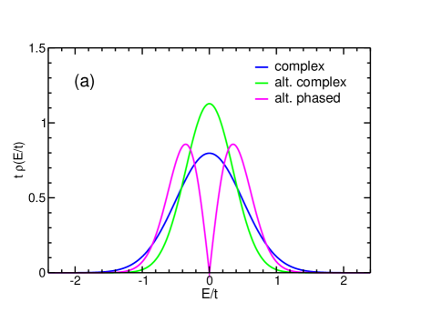
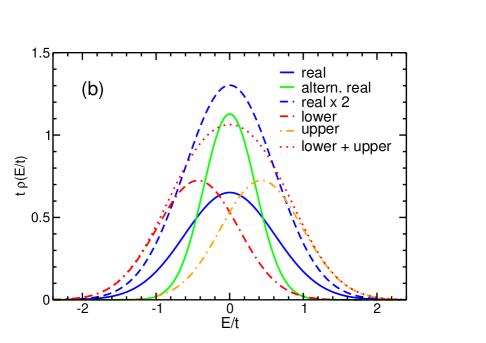
fully characterized by its (dimensionless) width , or is derivable fairly simply from Gaussians. For the above dispersions Eqs. (28) and (33) the DOSs are Gaussians with widths and , respectively, while for the dispersion (34) one finds that the DOS is a symmetrized Rayleigh distribution [88],
| (36) |
These three complex-orbital DOSs are shown for the full orbital case, i.e. , in Fig. 2(a) by the blue, green, and purple line, respectively.
III.2 Real-orbital single-particle states
For the single-particle states with real orbitals as defined by Eq. (12) with or , and for the single-particle states describing alternating real flavors and on the sublattices defined in the same way as above by Eqs. (29)–(32), one finds the dispersions
| (37) | |||||
| (38) | |||||
| (39) | |||||
One observes that, as already indicated at the very end of Sec. II.2, the sets of real-orbital single-particle states and are equivalent in the limit , in the sense that they have the same energies be it at opposite . As above for the complex-orbital single-particle states the alternating real-orbital single-particle states correspond to a lower () and an upper () band in the (reduced) Brillouin zone, both doubly degenerate, and their dispersions are proportional to , stemming entirely from the orbital-flavor non-conserving part of the kinetic energy.
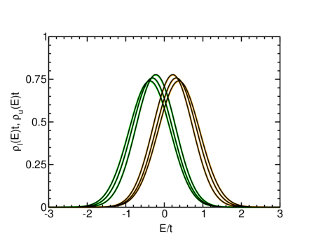
The corresponding DOSs are again Gaussians, with widths and , respectively, where ). They are shown, for , in Fig. 2(b) by the blue and green line respectively. One may note that , implying that the DOS of the alternating real-orbital single-particle states is identical to that of its complex-orbital counterpart shown in the upper panel.
III.3 Single-particle eigenstates
The creation operators for the single-particle eigen-states of the kinetic energy are seen from Eq. (20) to be simply proportional to the sum and difference of the phased single-particle operators,
| (40) | |||
| (41) |
and the corresponding energies of the lower () and upper () subbands are
| (42) |
where the () sign corresponds to the lower (upper) subband. We calculate the DOSs for the two subbands by evaluating the convolution of the DOSs corresponding to and to the two branches of . Strictly this requires and to be uncorrelated [88], which is obviously not the case because both depend on , but we assume that this condition becomes irrelevant in the limit , and check the validity of this assumption afterwards (see below). We then obtain for the subband DOSs
where the upper (lower) sign corresponds to the () subband, and for their sum, which we will need later,
| (44) | |||||
These DOSs are also shown, for , in Fig. 2(b) by the dash-dotted red and orange lines and by the dotted red line, respectively.
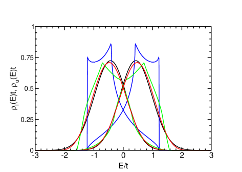
We emphasize that the subbands are non-degenerate except for the -points for which . This feature found already at dimension is generic and persists at increasing dimension up to , contrary to the suggestion made in Ref. [89]. Figures 3 and 4 demonstrate this explicitly. In Fig. 3 the DOSs of the two subbands are seen to become smoother with increasing dimension but to remain distinct although they partly overlap. In Fig. 4 the evolution of the subband DOSs with is illustrated: in the spin Hubbard model, i.e., at (not shown) they necessarily coincide, compare Eq. (42), while they are seen to get separated with their maxima moving away from each other with increasing and their maxima finally reaching a maximum distance of at (not shown), i.e., in the full orbital model. This figure also demonstrates the validity of our assumption made in deriving Eq. (III.3): the colored lines, calculated by -space sampling of the dispersion Eq. (42) at -values, are indistinguishable from the black lines, calculated from the analytical expression Eq. (III.3).
We point out that the single-particle eigenstates given by Eqs. (40)-(41) are in fact real and could be considered as the “phased” real-orbital single-particle operators which are the counterpart to the phased complex-orbital single-particle operators defined by Eq. (19) above,
| (45) | |||||
| (46) |
as one readily verifies from Eqs. (19) and (1), or alternatively by recognizing that Eqs. (40) and (41) have the form of coherent orbital states like Eq. (4) with and thus are given by Eq. (6). So they are represented in the “equatorial” plane, compare Fig. 1(c), by an angle equal to the phase angle , which is entirely determined by the wavevector and therefore is in general not equal to any of the . An important consequence is that each of these single-particle states carries a finite orbital polarization, i.e., contributes at each lattice site to the value of the pseudospin in the -plane, see Fig. 1(b),
| (47) | |||||
| (48) | |||||
| (49) |
It is noteworthy that while “” and “” may properly be called (sub)bands, the polarization direction of the states in each band varies with , in contrast to the familiar feature of bands of particles carrying spin where the spin direction is the same for all states in a band.
III.4 Comparison with the spin Hubbard model
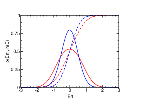
The expression (44) derived for the combined DOS of the two subbands gives us the opportunity to compare the distribution of the single-particle eigenstates in the orbital Hubbard with the one in the spin Hubbard model, see Fig. 5. In the orbital model the total DOS is broader and the total electron density grows slower with increasing Fermi energy . The plot already indicates that the kinetic energy in the orbital model at a particular density , obtained by filling the two subbands up to the same Fermi energy, is lower than the kinetic energy obtained at the same density in the spin model. This difference is a manifestation of the flavor non-conserving hopping which opens an extra channel for the kinetic energy and thus enhances it in the orbital model.
III.5 Kinetic energies
Before taking electron correlations into account, we examine the kinetic energy of the various trial states built from the single-particle states discussed above, and identify the most favorable states in the absence of Coulomb interactions. We consider on the one hand uniformly polarized ordered states, obtained by filling a single band (or, in the cases of alternating order, subsequently the lower and upper band corresponding to the same sublattice occupation), and on the other hand unpolarized “para-orbital” states, obtained by filling two degenerate bands up to the same Fermi energy, compare Eq. (27). For each such trial state the particle density and the kinetic energy as a function of the Fermi energy are given by
| (50) | |||||
| (51) |
where is the DOS of the corresponding band(s) of single-particle states. Only the density range will be considered since and are equivalent because of particle-hole symmetry.
We begin with the ordered orbital phases built from complex-orbital single-particle states. The simplest one is the complex ferro-orbital state obtained by filling the -band (or the -band). The complex alternating-orbital state is, compare Eqs. (31) and (32), obtained by filling consecutively the -band and the -band, and the phased complex alternating-orbital state is built similarly from the and single-particle states.
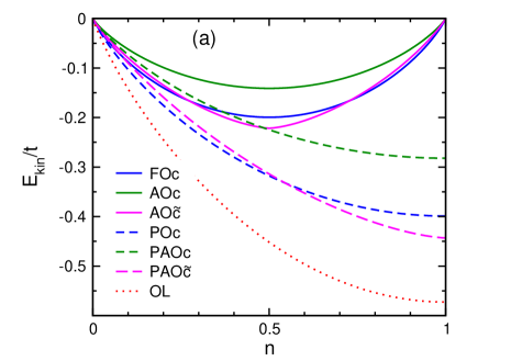
Moving on to the unpolarized states we have the complex para-orbital state POc, obtained by filling simultaneously the - and the -band, the complex alternating para-orbital state PAOc, by filling simultaneously the -band and the -band, compare Eq. (31), i.e., from the lower band only, and finally the similarly defined complex phased alternating para-orbital state PAO. Figure 6(a) shows the kinetic energies of these six states plotted versus the particle density.
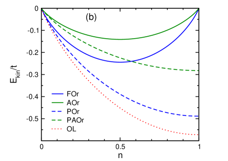
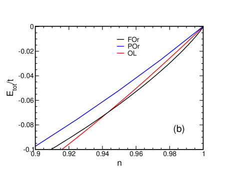
Next we consider the trial states built from real-orbital single-particle states, again beginning with the ordered phases. Analogous to the complex trial states above we have the real ferro-orbital state obtained by filling the -band (or alternatively the -band) and the real alternating-orbital state obtained by filling consecutively the -band and the -band, compare Eqs. (31) and (32). Here the unpolarized states are the real para-orbital state POr, with equally filled -band and -band, and the real alternating para-orbital state PAOr, with the -band and the -band filled equally. The kinetic energies of these four states plotted versus particle density are shown in Fig. 6(b).
The -dependence of the various kinetic energies can be understood as follows. For all ordered states for which the single-particle DOS is Gaussian, which includes the FOc, AOc, FOr, and AOr states, the particle density and kinetic energy take the form
| (52) | |||||
| (53) |
where is the error function. Formally, inversion of Eq. (52) gives
| (54) |
where is the inverse error function, and inserting this into Eq. (53) one obtains
| (55) |
This demonstrates that the shape of is the same for the states mentioned above, as is evident in Fig. 6, and that the only difference is in the width prefactor , which also determines the value of the minimum, , at . The only exception is the AO state for which the Rayleigh distribution type DOS Eq. (36) leads to
| (56) | |||||
| (57) | |||||
As Fig. 6(a) shows, this makes the AO state have lower kinetic energy than the FOc state close to quarter-filling, i.e., in the interval . This can be understood from the fact that the DOS of the phased complex-orbital single-particle states has more weight at more negative energies, see Fig. 2(a). However, as seen in Fig. 6(b), it is the FOr state that clearly has the lowest kinetic energy of all ordered states due to its large width, with minimum energy , whereas the minimum for the AO state is only , see Eq. (57). The basic reason for the difference is that the FOr state benefits fully from the orbital-flavor conserving hopping channel and also partially from the non-conserving channel, compare Eq. (37), while the AO state benefits fully from the orbital-flavor non-conserving channel but not at all from the conserving channel, cf. Eq. (34).
As regards the unpolarized states one may observe that for every para-orbital state PX its kinetic energy is related to that of the associated ordered state X by
| (58) |
which follows directly from the defining equations (50) and (51). Equation (58) implies that the relative magnitude of the kinetic energies of the unpolarized states is the same as that of the ordered states, as indeed seen in Fig. 6. In particular, the POr state has the lowest kinetic energy of all para-orbital disordered phases, for the same reason as the FOr state is the lowest-energy ordered state. Also, the para-orbital states have considerably lower kinetic energy than their ordered counterparts, but they will get renormalized at finite whereas the ordered states will not.
Finally we consider the trial state built from the single-particle eigenstates by filling the lower and the upper subband up to the same Fermi energy, written down here explicitly, compare Eqs. (40) – (42),
| (59) |
This state we call the OL state because it is unpolarized in the following remarkable way.
Whereas all single-particle states in are polarized individually, compare Eqs. (47) and (48), the variation with makes their contributions to the pseudospin add up to zero at each lattice site, at any filling and for each subband and separately. This follows from the following considerations (for a more detailed proof, see the Appendix): (i) for every single-particle state from the lowest subband which is occupied in because it satisfies , all single-particle states with wave vectors generated from by successive cyclic permutations of its components are also occupied; this holds because both and are invariant under such permutations, compare Eqs. (14) and (16), implying that , and it follows that ; the same reasoning applies for the upper subband ; (ii) under each such transformation the corresponding phase angle is transformed as , so summing over all yields , and the compensation of the contributions to the pseudospin follows, compare again Eqs. (47) and (48). Therefore, even though the densities in the two partially filled subbands are different, , as recognized from the DOSs shown in Fig. 2(b), the OL state is unpolarized, because each subband is unpolarized by itself at any filling. This mechanism is entirely different from the compensation of two oppositely polarized bands at equal filling as occurs for para-orbital (or paramagnetic) states.
We emphasize that the reasoning above is not specific for but holds in any dimension, and so the resulting absence of polarization in both bands is a characteristic feature of the OL per se. It is associated with the fact that the OL transforms as under the symmetry group (is invariant under U(1) in the limit ) and implies that the OL phase protects the (hyper)cubic symmetry. — We further point out that there is necessarily double occupancy in . This is obvious from the fact that the single-particle states in do not correspond to a single common direction in the ‘equatorial’ plane of Fig. 1(c) because of the variation of with the wave vector .
The relevant DOS from which to obtain the particle density and the kinetic energy in the OL state is , Eq. (44). One finds
| (60) | |||||
| (61) |
where
| (62) |
The function has to be calculated numerically. Since [90], we have rewritten Eq. (62) at as
| (63) |
to perform the calculation for the full orbital case.
The kinetic energy of the OL state is included in both Fig. 6(a) and Fig. 6(b), and is seen to be lower than that of any other trial state, remarkably including the lowest-energy complex-orbital and real-orbital para states. The explanation is similar to that above for the FOr and the POr states. The OL state fully captures all kinetic energy available in the orbital Hubbard model Eq. (9), both from the orbital-flavor conserving hopping channel and from the non-conserving hopping channel, cf. Eq. (42). This is a strong hint that the OL phase could be favored also in the presence of electron interactions. To establish the phase with the lowest overall energy we need to consider the energy renormalization of the para-orbital states and the OL state in the presence of the Coulomb interaction, i.e., at finite .
IV Correlations by the Gutzwiller method
The original analysis of the Gutzwiller approach in the limit , including the proof that the Gutzwiller approximation becomes exact in that limit, was carried out specifically for the spin Hubbard model, implying the implicit assumption of SU(2) symmetry [3, 8, 9]. We therefore need to investigate which modifications are required in the orbital case where we have only symmetry, and check if the proof of exactness still holds.
IV.1 General derivation at dimension
Electron correlations due to the on-site Hubbard repulsion will be implemented using the wave function introduced by Gutzwiller,
| (64) |
with
| (65) |
where the variational parameter is determined by minimizing the energy [6, 7, 8, 9],
| (66) |
First, we consider here the general case and derive the propagator and self-energy. In the present case the fermion (orbital) flavor is not conserved and we introduce a propagator,
| (67) |
which we allow to have, at least in principle, nonzero offdiagonal matrix elements with respect to flavor (i.e., ). Following Metzner [9], one finds the following expression for the matrix elements,
| (68) | |||||
where
| (69) |
Similarly, the bare propagator is defined by,
| (70) |
Here is, like , an matrix with off-diagonal elements with respect to orbital flavor generated by the off-diagonal hopping in orbital space. We emphasize that the curly brackets in Eqs. (68) and (70) denote the sum over all connected products of anticommuting contractions, evaluated in the trial state , and thus the (, etc.) symbols are Grassman variables and not the fermion operators (, etc.).
Next we define the self-energy . Here is a matrix with off-diagonal elements in orbital space. The elements of the self-energy are therefore different from those for the RVB wave function [9], and include the specific last term below,
| (71) | |||||
The self-energy gives the double occupancy,
| (72) |
The further derivation, following closely the case of the RVB state considered by Metzner [9], leads after some algebraic manipulations to the propagator in real space between sites and ,
| (73) | |||||
Here in the first local term at site only the diagonal elements of the matrix contribute, as indicated by .
The first term in Eq. (68) is related to the self-energy by
| (74) |
Finally, we define a “proper self-energy” as the sum over all one-particle irreducible diagrams contributing to —the two self-energies are then related by a Dyson equation,
| (75) |
After introducing a renormalized propagator
| (76) |
one finds that, owing to Eq. (75), it satisfies
| (77) |
The site-diagonal matrix elements of are related to those of as follows,
| (78) | |||||
| (79) |
IV.2 Single-site collapse at
Similar to the spin Hubbard model at , the diagrams describing the perturbation expansion of with respect to the local interaction collapse. Then the lattice sums reduce to summations of terms in which all indices coincide on the same lattice site, and the proper self-energy becomes site-diagonal, i.e., , The collapse permits the matrix elements of (with respect to the orbital label) to be expressed in terms of those of the on-site matrix elements of defined above. One finds in matrix form,
| (80) |
We emphasize that is not yet necessarily independent of . Here the factor is
| (81) |
and upon inversion,
| (82) |
Equating this to the site-diagonal part of as obtained from Eq. (77) generates two equations which together determine , for any given and . Next, Eq. (75) gives the self-energy , which finally determines the propagator via Eq. (73) and the double-occupancy using Eq. (72), and thus the total energy at any given electron filling .
IV.3 Momentum space representation
As we shall be mainly interested in translation invariant states, it is expedient to Fourier transform all variables of interest upon which matrix products with respect to site indices turn into ordinary products in -space, e.g. Eq. (73) becomes
Consider now a homogeneous state where is site-independent, and we may use a shorthand notation for its matrix elements,
| (84) |
Using the Dyson equation for in Eq. (77), can be expressed (in -space) explicitly in terms of and ,
| (85) |
where the normalizing prefactor is
| (86) |
It depends on the occupancy of the single-particle states at wave vector in the many-particle trial state . Upon solving for , , , and , one obtains the self-energy from
| (87) |
upon which it is straightforward to write down explicitly the expression for the propagator and calculate all quantities of physical interest.
V Gutzwiller renormalization
V.1 Ordered states
As an example, we consider an ordered, i.e. polarized, state with complex orbitals, Oc,
| (88) |
It contains fixed numbers of electrons and in and states (), respectively,
| (89) |
which determine the total electron number and orbital polarization ,
| (90) |
The state (88) includes both full polarization, and , i.e., the complex ferro-orbital state FOc, and zero polarization, , , i.e., the complex para-orbital state POc.
The bare propagator is a diagonal matrix in the orbital basis, i.e., , and thus . Consequently, the explicit form of the matrix elements of and simplify, and the equations following from Eqs. (85) and (82) reduce to
| (91) | |||||
| (92) | |||||
| (93) | |||||
From Eq. (92) it follows that , and Eqs. (91) and (93) are simplified to
| (94) | |||||
| (95) |
where is the number of singly occupied -points of flavor and is the number of doubly occupied -points, hence
| (96) |
After some algebraic manipulation one finds
| (97) |
and the solution for and can be found.
Using the simplified (because of ) expressions for and one finds,
| (98) |
with
| (99) | |||||
| (100) |
This is the Gutzwiller approximation for the ordered state Eq. (88). Note that
| (101) |
i.e., Luttinger theorem is satisfied. The average double occupancy is given by
| (102) |
One recognizes that the above results are identical to those obtained in the spin case, i.e., for SU(2) symmetry.
For any other trial state built from a single pair of orthogonal orbitals, cf. Eq. (4),
| (103) |
one obtains exactly analogous results when similarly writing all expressions in terms of the corresponding orbital basis. So, e.g. for the real Or states built from and single-particle states, compare Eq. (88), one has
| (104) |
compare Eq. (98). The renormalization and the background constant density are straightforwardly obtained from and by the corresponding orbital transformation.
V.2 Orbital liquid state
Next we consider the OL state introduced above, see Eq. (59),
| (105) |
where and label the occupied states from the lower () and upper () subband, and both subbands are occupied up to the same Fermi energy .
The free propagator is, in the basis,
| (106) |
This leads to the following expressions for the on-site matrix of in real space, ,
where the normalizing prefactor depends on the occupancy of the subbands at wave vector : it equals if only a single (viz. the lower) subband is occupied and equals if both and are occupied, with
| (110) | |||||
| (111) | |||||
Setting the expressions above equal to those obtained in Eq. (82) one obtains a set of four equations from which to determine , , , and .
Because of the occurrence of the phases in Eqs. (V.2) - (V.2) these equations cannot be solved in full generality and a simplifying assumption is necessary. Thus we make here the ansatz that the off-diagonal elements of vanish, i.e., . Then the terms that involve summation over the phase factors drop out and the structure of the equations needed to determine simplifies. Because the OL state is not polarized the two flavors are equivalent and the diagonal elements of must be equal, . Defining single and double occupancy in -space per -point,
| (112) | |||||
| (113) |
one obtains a single equation for in terms of and ,
| (114) |
Using the number of electrons per site , one finds finally for the orbital liquid state
| (115) |
Inserting this result into the expressions for the renormalization factor and double occupancy in terms of ,
| (116) | |||||
| (117) |
one finally obtains
| (119) |
This expression for the kinetic energy renormalization (V.2) is identical to that which follows from Eq. (99) when the ordered state is unpolarized, i.e., for . At one finds and
| (120) |
which reproduces the kinetic energy renormalization in the spin model.
VI Brinkman-Rice transition
In the following we focus on the OL state, and in particular compare its role in the orbital Hubbard model with that of the paramagnetic phase in the spin Hubbard model. For the latter purpose it is convenient to introduce – then the results obtained here at for orbital phases are directly comparable with those for magnetic phases [11].
Altogether the energy of the OL is determined by
| (121) |
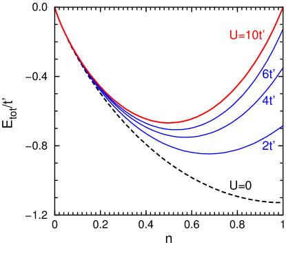
and one has to use Eqs. (V.2) and (119) with the optimal value of the variational parameter . The result for the density dependence of for the OL phase is shown in Fig. 7 for a number of values of . One observes that the renormalization of the kinetic energy due to electron correlations induced by is largest at half-filling, i.e., at . Indeed, here one might expect an insulating state to appear eventually at sufficiently large , with completely suppressed electron dynamics, see below. Further, with increasing the total energy (121) gradually increases at any density and its minimum moves towards . The pattern seen in Fig. 7 is entirely similar to that shown by the paramagnetic phase in the spin Hubbard model when treated likewise by the Gutzwiller method, because it is dominated by the behavior of and and hardly affected by the slight difference in the shape of .
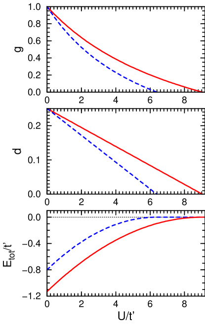
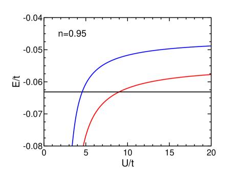
Figure 8 shows in some more detail what happens at , demonstrating that for the OL in the orbital model the dependence of the variational parameter , the double occupancy , and the total energy on is qualitatively the same as for the paramagnetic state in the spin model. In particular double occupancy gets fully suppressed () at and above a critical value , while simultaneously implying , i.e., the electrons are entirely localized and itinerancy disappears. This has been recognized in the spin case by Brinkman and Rice [91] as a qualitative criterion for the onset of the transition from a metallic to an insulating state [92], which in fact becomes exact at [93].
However, quantitatively there is a considerable difference: for the OL in the orbital Hubbard model this transition occurs at , enhanced from for the paramagnetic state in the spin Hubbard model (equivalent to the () POc state in the orbital model), because is generally given by
| (122) |
which is larger by the factor for the OL, compare Eqs. (61) and (53). Clearly this is entirely due to the extra contribution to the kinetic energy coming from the orbital-flavor non-conserving hopping at . We note in passing that the real para-orbital phase POr shows a Brinkman-Rice transition at the intermediate value , enhanced only by a factor , because it profits only partially from the additional kinetic energy available in the orbital model.
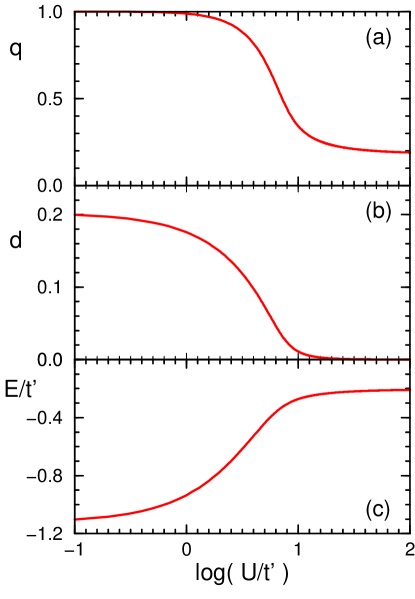
At the renormalization factor , Eq. (V.2), remains finite at large , and thus the electrons remain itinerant, be it with reduced kinetic energy, see Fig. 9. Increasing defines here three distinct regimes: (i) at very small () correlations are virtually absent, and , (ii) at small () the correlations gradually develop, is reduced from 1.0 down to , double occupancy is strongly reduced (), and the total energy increases, and (iii) at large () the correlations dominate, double occupancy becomes excluded and the electrons move in the strongly correlated OL without creating double occupancies.
VII Phase diagram
From the unrenormalized kinetic energies shown in Fig. 6 we concluded that the uniformly polarized FOr phase and possibly the disordered POr phase are the only candidates competing with the OL phase for being the ground state after the energies of the POr and OL phase have been renormalized by correlations, for the following reasons: First, as double occupancies do not occur in the FOr phase or the other uniform phases with broken symmetry, these phases are not affected by renormalization and so the sequence of their energies is fixed. Second, although the energies of the disordered phases are changed by accounting for correlations, their sequential order also cannot change if all of them are subjected to the same renormalization procedure (at least if the procedure is only sensitive to energies as is the case for the Gutzwiller method). This holds because for any phase its total renormalized energy is given by an expression like Eq. (121) with the variational parameter(s) optimized for the lowest outcome; if the kinetic energy in this equation is replaced by a lower value associated with a different phase, the total energy is lowered even if the variational parameter is kept fixed; subsequently allowing to optimize can only lead to a further lowering of the total energy. This argument should not only hold for the para-orbital phases but also be valid between the POr and OL phases, implying that the only competition of interest should be between the FOr phase and the OL phase.
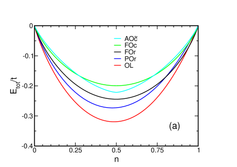
Numerical results are shown in Fig. 10(a) for the dependence upon density of the total energies of various phases at a particular value of , viz. . The states other than the FOr and the OL states are included here just to demonstrate that they do not play a role, as argued above. Yet indeed, a competition between the FOr phase and the OL does take place and the total energies of these phases are seen to be quite close to one another. In fact they cross and, whereas the energy of the OL is well below that of the FOr state over most of the density range even for this rather large value of , the OL phase is unstable against the FOr phase close to , as shown in more detail in Fig. 10(b). We point out that the latter result is different from that obtained for the 3D orbital Hubbard model (at ) where the OL is stable in the entire regime of also at large [13].
The transition between the OL phase and the FOr phase can be determined more accurately by calculating at fixed the total energy of the OL as a function of and comparing this with the -independent total energy of the FOr state, as shown in Fig. 11. One thus obtains where the two phases have equal energy. This defines the OL-FOr phase boundary because the transition is first-order, since the states and cannot transform continuously into one another because of the globally different structure of and . This stands in clear contrast to the paramagnetic-ferromagnetic transition in the spin Hubbard model, which is second order because the magnetization can evolve gradually from the paramagnetic state.
The resulting phase diagram of the orbital Hubbard model in the (, ) plane as obtained in the Gutzwiller approximation is shown in Fig. 12. The FOr phase is more stable than the OL phase for if . Here is the critical value of the particle density at which the energies of the phases are equal at , and below which the OL is therefore always stable, see Fig. 12. It is obtained from a numerical comparison using the analytical expressions for the kinetic energies of the two phases, Eq. (55) and Eq. (61), and for the renormalization factor at , Eq. (120).
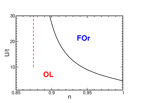
Next we consider the intersection of the phase boundary with the -axis at . With our simple representation of real-orbital ferro order by the state , which has fully saturated orbital order such that independent of , this intersection necessarily coincides with the Brinkman-Rice transition point where the energy of the OL attains , so . However, as pointed out by Fazekas et al. for the spin case [11], precisely close to a small reduction of the polarization must occur involving the exponential tails of the DOSs of the - and -bands. If this would be taken into account it would produce some lowering of the energy of the FOr phase thus leading to a slight decrease of .
Allowing some polarization of the FOr state at general density, at the price of creating double occupancy, would similarly give some energy lowering. However, this is severely limited by the restriction that upon transferring one particle from the majority to the minority band the gain in kinetic energy must exceed . This condition is only met as long as the Fermi energy of the minority band is in the exponential tail of the DOS, i.e. only for a very small fraction of the particles, and also , compare Fig. 2(b). Thus our use of the fully ordered state neglects at most a minor expansion of the FOr regime in the phase diagram.
We have not attempted to construct a more sophisticated trial state for any of the AO phases, such as has been shown to be important to obtain a good description of the AF phase in the spin Hubbard model [8, 11]. So, strictly we cannot exclude that alternating orbital order would show up in the orbital model at and/or close to half-filling by outcompeting the ferro orbital order, as occurs between antiferromagnetism and ferromagnetism in the spin case. However, this seems unlikely in the orbital case because of the large difference in kinetic energy between the fully ordered states, see Fig. 6, viz. by a factor between the FOr and AOr states, and (because the kinetic energy of the AO state is very close to that of the FOc state) by a factor between the FOr and AO states. As shown above, this difference is due to the more efficient use of both pseudospin-conserving and non-conserving hopping channels by real-orbital ferro order than by alternating orbital order. What we do have established is that the OL state is the ground state over most of the () phase diagram, as illustrated by Fig. 12.
Finally, we point out that the phase diagram obtained here at is qualitatively different from that found before at [13]. In the latter case the lowest-energy ordered FOx phase was completely eliminated from the phase diagram by the non-conserving hopping, and the OL phase was the only phase present. We propose that this is caused by the different energy ranges: at versus at . The argumentation is as follows:
Let us consider, at , the derivatives with respect to of the total energy of the candidate phases (viz. FOr and OL at , FOx and OL at ) at , as these determine which phase has the lowest energy in the immediate vicinity of half-filling, compare Fig. 10. Since at , we have and , compare Eq. (121), and therefore
| (123) | |||||
| (124) | |||||
Both expressions can be evaluated, (i) at : by consulting [13], for the FOx phase using Eq. (3.23) therein (from which one obtains and thus ), for the OL phase making use of the data plotted in Fig. 5 therein [from which one obtains and ]; (ii) at : for the FOr phase using Eqs. (54) in the present paper with , for the OL phase using Eq. (61) and so obtain ; (iii) inserting and .
The results are as follows:
| (125) | |||||
| (126) | |||||
| (127) | |||||
| (128) |
So, for the derivative is slightly larger for the OL, implying that close to this is the lowest state and then will remain so in the entire phase diagram, as we found before [13]. However, for the slope for the FOr phase initially diverges (the function at ), so the FOr state is the ground state close to , as we found in the present paper. This divergence is not seen in the plots because it is very steep. Thus already for larger than the derivative is of order 1 and with further increasing the FOr phase begins to be overtaken by the OL. So the reason for the FOr phase being stable at apparently lies in the exponential tails in its DOS, particle density and kinetic energy. As this is a mathematical rather than a physical phenomenon, the above result suggests that stability of ordered phases at is mathematically correct but physically spurious, and that the earlier theoretical result at [13] describes the generic physics.
We thus conclude that regarding the phase diagram the case is not representative for all dimensions: the case is qualitatively different. This actually demonstrates that the effect of the non-conserving hopping terms themselves is qualitatively different for different dimensions, which is not the case for the conserving terms, since FM and AF phases appear in the phase diagram of the spin Hubbard model in all dimensions.
VIII Discussion and conclusions
VIII.1 General aspects of the orbital model
A few aspects of the orbital Hubbard model at deserve some further comments. They mainly concern the limitations of the Gutzwiller approach in comparison with more powerful recent methods, in particular selfconsistent DMFT. As mentioned briefly in Sec. I the development of the DMFT approach [62] was made possible by the discovery by Metzner and Vollhardt that in the limit only on-site correlations survive [8]. Nowadays DMFT is recognized as a standard method to study electron correlation effects in the electronic structure [94, 95, 96, 97]. This method has been successfully applied, inter alia, to the Falicov-Kimball model [98] and to nonequilibrium dynamics [99]. The ideas employed using the Gutzwiller wave function helped to formulate the DMFT method in spin systems [95].
First of all, one may wonder to what extent the description of the metal-insulator transition, as presented in Sec. VI, i.e., as a Brinkman-Rice transition, is realistic. An additional aspect for the orbital model are possible crystal-field splittings but it has been established that orbital-selective Mott phases occur then for large enough interaction [100, 101]. However, when the orbitals remain equivalent as in the OL state considered in the present paper, one may expect that the transition occurs in a similar way as in the paramagnetic state in the spin model. So our treatment of the metal-insulator transition in the orbital model at by the Gutzwiller approach, leading to the Brinkman-Rice transition, then has the same status as the treatment of the metal-insulator transition in the spin model at by that same approach, and gives valuable insight how correlations induce the system to approach the localized state [95].
Second, past calculations using the Gutzwiller wave function have led to a better understanding of the strongly correlated regime of the Hubbard model. In one dimension the metal-insulator transition is absent but several quantities have been calculated exactly [102]: the double occupation, the momentum distribution, as well as its discontinuity at the Fermi surface. These quantities determine the expectation value of the 1D Hubbard Hamiltonian for any symmetric and monotonically increasing dispersion. The Gutzwiller wave function has also been found to predict ferromagnetic behavior for sufficiently large interaction [103, 104]. This agrees with the present result that the orbital Hubbard model also has a range of ferro-orbital states close to .
However, it has been known for some time that the Brinkman-Rice picture of the metal-insulator transition, as given by the Gutzwiller approach both at and at , is oversimplified, in particular yielding a poor description of the dynamics on the insulating side [105]. Recent studies of the metal-insulator transition in the spin Hubbard model at by DMFT have demonstrated the existence of two different transitions, a metal-to-insulator transition at where the quasiparticle weight becomes zero and an insulator-to-metal transition at where the gap closes, both first-order, and the occurrence of hysteresis between the two critical interaction strengths [106, 107, 108]. This holds from up to a critical temperature where and coalesce, while for there is a smooth crossover between metallic and insulating behavior. Notably, the thermodynamics of the hysteresis region was recently explained at the two-particle level [109]. Obviously, the above more-detailed understanding of the Mott-Hubbard transition implies that this transition is considerably more complex than the Brinkman-Rice picture suggests.
These differences between the Mott-Hubbard transition in the spin Hubbard model as calculated by DMFT and the Brinkman-Rice picture are clearly due to the fact that DMFT is coping more effectively with correlations than the Gutzwiller approach. One would therefore expect that a DMFT treatment of the orbital Hubbard model would produce similar changes to the metal-insulator transition as in the spin Hubbard model, because this transition is typically a correlation-induced phenomenon. By contrast, one would expect the more prominent role of the disordered OL in the phase diagram (as compared to the paramagnetic phase in the spin case) to remain largely unaffected, because it is not due to correlations but to the additional kinetic energy provided by the non-conserving hopping channel.
However, these are just speculations. We emphasize that orbital models such as that in Eq. (9) [or Eq. (7)] have as yet not been studied in the context of self-consistent DMFT calculations. Therefore, even the corresponding effective impurity model for such calculations is not known, and its construction appears not to be entirely trivial. A prime candidate is a two-orbital Anderson impurity model with on-site and selfconsistently generated orbital flipping terms. In view of the overriding importance of the orbital non-conserving hopping channel and the associated symmetry demonstrated above, these features should apparently be incorporated somehow. The only way seems to be by imposing a specific structure on the bath modes and their coupling to the impurity. It would be desirable if a DMFT treatment along these lines were performed, both to see if the above speculations on the orbital Hubbard model are born out and to further explore the application of the DMFT method to a wider range of models.
The early ideas of Kugel and Khomskii [19] culminate in systems where spins and orbitals become almost equivalent. This idealization happens for face-sharing octahedra and one finds indeed a highly symmetric SU(4) model [110]. So far, studies of such systems have only been performed theoretically and these have identified an interesting evolution of spin-orbital entanglement with increasing spin-orbit coupling [66]. In spite of the absence of long-range spin-orbital order such systems exhibit features typical of those manifesting themselves at phase transitions [111]. The experimental search for quantum spin-orbital liquids identified FeSc2S4 as a quantum material with long-range entanglement [112]. Such states are primarily realized in the Kitaev materials where spins and orbitals lose their identity and are strongly entangled by large spin-orbit coupling [113]. The challenge in the theory is to find a quantum spin-orbital liquid at infinite dimension.
VIII.2 Summary
Summarizing, we have presented a generalization of the orbital model to infinite dimension , preserving the two-fold degeneracy of the orbitals and turning the lattice symmetry from cubic into hypercubic. It is quite remarkable that the two-flavor orbital model is manifestly different from the corresponding spin model at by the presence of orbital-flipping hopping terms. At the same time it is somewhat surprising that the two orbital flavors are equivalent in the limit of when they are so different in the 3D model, including the physics of the manganites [80]. We have further shown that the Gutzwiller approximation becomes exact in the limit for the orbital Hubbard model in perfect analogy with the spin Hubbard model.
We conclude that the peculiar features of the orbital Hubbard model (9) are due to the fact that the extra hopping terms do not conserve the pseudospin as they mix the two orbital flavors. They thus induce the following distinctive features: (i) there are two classes of single-particle plane-wave states: those with complex orbitals and those with real orbitals, which behave differently; the same holds for the Fermi-sea-like multiparticle states built from them; (ii) the single-particle eigenstates of the kinetic energy form two distinct bands with different dispersions; (iii) each such eigenstate carries a nonzero polarization, i.e., contributes to the pseudospin at all sites; yet when summed over all eigenstates in an energy shell, these contributions add up to zero; by this mechanism the orbital liquid state (OL), which is obtained by filling the two bands of single-particle eigenstates to the same Fermi energy, is unpolarized at any filling. The above qualitative features are generic for the orbital Hubbard model, i.e., they hold at any dimension, from up to .
There are also a number of features induced by the non-conserving hopping channel that are to some extent quantitative and are most pronounced at . (iv) The extra hopping channel lowers the kinetic energy with respect to the spin case and thus makes the Brinkman-Rice transition to an insulator occur at a larger value of ; (v.a) phases with alternating orbitals are much less favored than antiferromagnetism for fermions on a bipartite lattice like the hypercubic lattices considered here, because they benefit relatively less from the pseudospin-conserving channel, whereas (v.b) unlike ferromagnetic states in the spin Hubbard model, ferro-orbital states are not eigenstates of the orbital Hubbard model (9) and benefit energetically more from the orbital-mixing term; (v.c) together this makes the FOr state the main competitor of the orbital liquid phase, and the phase diagram confirms that FOr order indeed occurs at large close to half-filling [114], while the orbital liquid phase is the ground state elsewhere; (v.d) the stability of the FOr is apparently due to the exponential tails in the DOS, particle density and kinetic energy, and so is specific for , whereas at the OL phase is the lowest-energy state in the entire phase diagram. Perhaps feature (v.a) is the most remarkable quantitative consequence of orbital physics. Having richer hopping processes both with and without the restriction that the orbital flavor is conserved, one has to accept that alternating orbital order is more difficult to realize than in the spin model [11]. Feature (v.b) makes it more difficult to realize fully polarized ferro-orbital states so it may sound surprising that nevertheless the FOr phase is more stable than the orbital liquid in a range of electron densities . Note that the theorem formulated by Nagaoka [115] at for the spin case does not apply to the orbital Hubbard model.
One of the attractive ideas in this field has been the possible existence of polarized ferro-orbital states with partly filled complex orbitals [116]. We have established that unfortunately such states cannot be realized. We have shown that they are unstable and one has to consider instead FOr states.
Acknowledgements.
We thank Walter Metzner for his interest and for very insightful discussions. L.F.F. thanks the Max Planck Institute for Solid State Research in Stuttgart and the Jagiellonian University in Kraków for their kind hospitality. A.M.O. kindly acknowledges Narodowe Centrum Nauki (NCN, Poland) Project No. 2016/23/B/ST3/00839 and is grateful for support via the Alexander von Humboldt Foundation Fellowship [117] (Humboldt-Forschungspreis). *Appendix A Proof that the orbital liquid phase is unpolarized
References
- [1] J. Hubbard, Electron Correlations in Narrow Energy Bands, Proceedings of the Royal Society of London A 276, 238 (1963).
- [2] P. W. Anderson, New Approach to the Theory of Superexchange Interactions, Phys. Rev. 115, 2 (1959).
- [3] W. Metzner and D. Vollhardt, Correlated Lattice Fermions in Dimension, Phys. Rev. Lett. 62, 324 (1989).
- [4] W. Metzner and D. Vollhardt, Analytic calculation of ground-state properties of correlated fermions with the Gutzwiller wave-function, Phys. Rev. B 37, 7382 (1988).
- [5] M. C. Gutzwiller, Effect of correlation on the ferromagnetism of transition metals, Phys. Rev. Lett. 10, 159 (1963).
- [6] M. C. Gutzwiller, Correlation of Electrons in a Narrow Band, Phys. Rev. 137, A1726 (1965).
- [7] D. Vollhardt, Normal He3 — An almost localized Fermi liquid, Rev. Mod. Phys. 56, 99 (1984).
- [8] W. Metzner, Variational theory for correlated lattice fermions in high dimension, Z. Phys. B 77, 253 (1989).
- [9] W. Metzner, Analytic evaluation of resonating valence bond states, Z. Phys. B 82, 183 (1991).
- [10] P. W. Anderson, Resonating valence bonds: A new kind of insulator?, Mater. Res. Bull. 8, 153-160 (1973).
- [11] P. Fazekas, B. Menge, and E. Müller-Hartmann, Ground state phase diagram of the infinite dimensional Hubbard model: A variational study, Z. Phys. B 78, 69 (1990).
- [12] S. Ishihara, M. Yamanaka, and N. Nagaosa, Orbital liquid in perovskite transition-metal oxides, Phys. Rev. B 56, 686 (1997).
- [13] L. F. Feiner and A. M. Oleś, Orbital liquid in ferromagnetic manganites: The orbital Hubbard model for electrons, Phys. Rev. B 71, 144422 (2005).
- [14] T. Tanaka, M. Matsumoto, and S. Ishihara, Randomly diluted orbital-ordered systems, Phys. Rev. Lett. 95, 267204 (2005).
- [15] T. Tanaka and S. Ishihara, Dilution effects in two-dimensional quantum orbital systems, Phys. Rev. Lett. 98, 256402 (2007).
- [16] P. Czarnik, J. Dziarmaga, and A. M. Oleś, Overcoming the sign problem at finite temperature: Quantum tensor network for the orbital model on an infinite square lattice, Phys. Rev. B 96, 014420 (2017).
- [17] L. Balents, Spin liquids in frustrated magnets, Nature (London) 464, 199-208 (2010).
- [18] L. Savary and L. Balents, Quantum spin liquids: A review, Rep. Prog. Phys. 80, 016502 (2017).
- [19] K. I. Kugel and D. I. Khomskii, The Jahn-Teller effect and magnetism: Transition metal compounds, Usp. Fiz. Nauk 136, 621 (1982) [Sov. Phys. Usp. 25, 231 (1982)].
- [20] D. I. Khomskii, Transition Metal Oxides (Cambridge University Press, Cambridge, 2014).
- [21] M. Imada, A. Fujimori, and Y. Tokura, Metal-insulator transitions, Rev. Mod. Phys. 70, 1039 (1998).
- [22] Y. Tokura and N. Nagaosa, Orbital Physics in Transition-Metal Oxides, Science 288, 462-468 (2000).
- [23] A. V. Gorshkov, M. Hermele, V. Gurarie, C. Xu, P. S. Julienne, J. Ye, P. Zoller, E. Demler, M. D. Lukin, and A. M. Rey, Two-orbital SU(N) magnetism with ultracold alkaline-earth atoms, Nature Phys. 6, 289 (2010).
- [24] A. Koga, N. Kawakami, T. M. Rice, and M. Sigrist, Orbital-Selective Mott Transitions in the Degenerate Hubbard Model, Phys. Rev. Lett. 92, 216402 (2004).
- [25] L. F. Feiner, A. M. Oleś, and J. Zaanen, Quantum Melting of Magnetic Order due to Orbital Fluctuations, Phys. Rev. Lett. 78, 2799 (1997).
- [26] L. F. Feiner, A. M. Oleś, and J. Zaanen, Quantum disorder versus order-out-of-disorder in the Kugel-Khomskii model, J. Phys.: Condens. Matter 10, L555 (1998).
- [27] G. Khaliullin and V. Oudovenko, Spin and orbital excitation spectrum in the Kugel-Khomskii model, Phys. Rev. B 56, R14243 (1997).
- [28] P. Corboz, M. Lajkó, A. M. Laüchli, K. Penc, and F. Mila, Spin-Orbital Quantum Liquid on the Honeycomb Lattice, Phys. Rev. X 2, 041013 (2012).
- [29] G. Khaliullin and S. Maekawa, Orbital liquid in three-dimensional Mott insulator: LaTiO3, Phys. Rev. Lett. 85, 3950 (2000).
- [30] G. Khaliullin, Orbital order and fluctuations in Mott insulators, Prog. Theor. Phys. Suppl. 160, 155 (2005).
- [31] K. Kitagawa, T. Takayama, Y. Matsumoto, A. Kato, R. Takano, Y. Kishimoto, S. Bette, R. Dinnebier, G. Jackeli, and H. Takagi, A spin-orbital-entangled quantum liquid on a honeycomb lattice, Nature (London) 554, 341 (2018).
- [32] L. F. Feiner and A. M. Oleś, Electronic origin of magnetic and orbital ordering in insulating LaMnO3, Phys. Rev. B 59, 3295 (1999).
- [33] J. van den Brink, P. Horsch, F. Mack, and A. M. Oleś, Orbital dynamics in ferromagnetic transition-metal oxides, Phys. Rev. B 59, 6795 (1999).
- [34] A. M. Oleś, G. Khaliullin, P. Horsch, and L. F. Feiner, Fingerprints of spin-orbital physics in cubic Mott insulators: Magnetic exchange interactions and optical spectral weights, Phys. Rev. B 72, 214431 (2005).
- [35] A. Reitsma, L. F. Feiner, and A. M. Oleś, Orbital and spin physics in LiNiO2 and NaNiO2, New J. Phys. 7, 121 (2005).
- [36] J. Chaloupka and G. Khaliullin, Orbital order and possible superconductivity in LaNiO3/LaMO3 superlattices, Phys. Rev. Lett. 100, 016404 (2008).
- [37] V. I. Solovyev, Spin-orbital superexchange physics emerging from interacting oxygen molecules in KO2, New J. Phys. 10, 013035 (2008).
- [38] B. Normand and A. M. Oleś, Frustration and entanglement in the spin-orbital model on a triangular lattice: valence-bond and generalized liquid states, Phys. Rev. B 78, 094427 (2008).
- [39] F. Krüger, S. Kumar, J. Zaanen, and J. van den Brink, Spin-orbital frustrations and anomalous metallic state in iron-pnictide superconductors, Phys. Rev. B 79, 054504 (2009).
- [40] W. Lv, F. Krüger, and P. Phillips, Orbital ordering and unfrustrated magnetism from degenerate double exchange in the iron pnictides, Phys. Rev. B 82, 045125 (2010).
- [41] B. Normand, Multicolored quantum dimer models, resonating valence-bond states, color visons, and the triangular-lattice spin-orbital system, Phys. Rev. B 83, 094427 (2011).
- [42] J. Chaloupka and A. M. Oleś, Spin-orbital resonating valence-bond liquid on a triangular lattice: Evidence from finite cluster diagonalization, Phys. Rev. B 83, 094427 (2011).
- [43] K. Wohlfeld, M. Daghofer, and A. M. Oleś, Spin-orbital physics for orbitals in alkali hyperoxides—Generalization of the Goodenough-Kanamori rules, EPL (Europhysics Letters) 96, 27001 (2011).
- [44] K. Wohlfeld, M. Daghofer, S. Nishimoto, G. Khaliullin, and J. van den Brink, Intrinsic Coupling of Orbital Excitations to Spin Fluctuations in Mott Insulators, Phys. Rev. Lett. 107, 147201 (2011).
- [45] J. Schlappa, K. Wohlfeld, K. J. Zhou, M. Mourigal, M. W. Haverkort, V.N. Strocov, L. Hozoi, C. Monney, S. Nishimoto, S. Singh, A. Revcolevschi, J.-S. Caux, L. Patthey, H. M. Ronnow, J. van den Brink, and T. Schmitt, Spin-orbital separation in the quasi-one-dimensional Mott insulator Sr2CuO3, Nature (London) 485, 82-U108 (2012).
- [46] K. Wohlfeld, S. Nishimoto, M. W. Haverkort, and J. van den Brink, Microscopic origin of spin-orbital separation in Sr2CuO3, Phys. Rev. B 88, 195138 (2013).
- [47] V. Bisogni, K. Wohlfeld, S. Nishimoto, C. Monney, J. Trinckauf, K. Zhou, R. Kraus, K. Koepernik, C. Sekar, V. Strocov, B. Büchner, T. Schmitt, J. van den Brink, and J. Geck, Orbital Control of Effective Dimensionality: From Spin-Orbital Fractionalization to Confinement in the Anisotropic Ladder System CaCu2O3, Phys. Rev. Lett. 114, 096402 (2015).
- [48] C.-C. Chen, M. van Veenendaal, T. P. Devereaux, and K. Wohlfeld, Fractionalization, entanglement, and separation: Understanding the collective excitations in a spin-orbital chain, Phys. Rev. B 91, 165102 (2015).
- [49] W. Brzezicki, A. M. Oleś, and M. Cuoco, Spin-Orbital Order Modified by Orbital Dilution in Transition-Metal Oxides: From Spin Defects to Frustrated Spins Polarizing Host Orbitals, Phys. Rev. X 5, 011037 (2015).
- [50] W. Brzezicki, M. Cuoco, and A. M. Oleś, Novel Spin-Orbital Phases induced by Orbital Dilution, J. Supercond. Novel Magn. 29, 536 (2016).
- [51] W. Brzezicki, M. Cuoco, and A. M. Oleś, Exotic Spin-Orbital Physics in Hybrid Oxides, J. Supercond. Novel Magn. 30, 129 (2017).
- [52] J. B. Goodenough, Magnetism and the Chemical Bond (Interscience, New York, 1963).
- [53] A. M. Oleś, P. Horsch, L. F. Feiner, and G. Khaliullin, Spin-Orbital Entanglement and Violation of the Goodenough-Kanamori Rules, Phys. Rev. Lett. 96, 147205 (2006).
- [54] A. M. Oleś, Fingerprints of spin-orbital entanglement in transition metal oxides, J. Phys.: Condensed Matter 24, 313201 (2012).
- [55] W. Brzezicki, J. Dziarmaga, and A. M. Oleś, Noncollinear Magnetic Order Stabilized by Entangled Spin-Orbital Fluctuations, Phys. Rev. Lett. 109, 237201 (2012).
- [56] W. Brzezicki, J. Dziarmaga, and A. M. Oleś, Exotic spin orders driven by orbital fluctuations in the Kugel-Khomskii model, Phys. Rev. B 87, 064407 (2013).
- [57] M. Snamina and A. M. Oleś, Magnon dressing by orbital excitations in ferromagnetic planes of K2CuF4 and LaMnO3, New J. Phys. 21, 023018 (2019).
- [58] W. Brzezicki, Spin, orbital and topological order in models of strongly correlated electrons, J. Phys.: Condensed Matter 32, 023001 (2020).
- [59] P. A. Lee, N. Nagaosa, and X.-G. Wen, Doping a Mott insulator: Physics of high-temperature superconductivity, Rev. Mod. Phys. 78, 17 (2006).
- [60] M. Ogata and H. Fukuyama, The - model for the oxide high- superconductors, Rep. Prog. Phys. 71, 036501 (2008).
- [61] B. Keimer, S. A. Kivelson, M. R. Norman, S. Uchida, and J. Zaanen, High Temperature Superconductivity in the Cuprates, Nature 518, 179 (2015).
- [62] A. Georges, G. Kotliar, W. Krauth, and M. J. Rozenberg, Dynamical mean-field theory of strongly correlated fermion systems and the limit of infinite dimensions, Rev. Mod. Phys. 68, 13 (1996).
- [63] J. Merino and R. H. McKenzie, Transport properties of strongly correlated metals: A dynamical mean-field approach, Phys. Rev. B 61, 7996 (2000).
- [64] B. Kyung, S. S. Kancharla, D. Sénéchal, A.-M. S. Tremblay, M. Civelli, and G. Kotliar, Pseudogap induced by short-range spin correlations in a doped Mott insulator, Phys. Rev. B 73, 165114 (2006).
- [65] G. Kotliar, S. Y. Savrasov, K. Haule, V. S. Oudovenko, O. Parcollet, and C. A. Marianetti, Electronic structure calculations with dynamical mean-field theory, Rev. Mod. Phys. 78, 865 (2006).
- [66] D. Gotfryd, E. Pärschke, J. Chaloupka, A. M. Oleś, and K. Wohlfeld, How Spin-Orbital Entanglement depends on the Spin-Orbit Coupling in a Mott Insulator, Phys. Rev. Research 2, 013353 (2020).
- [67] D. Gotfryd, E. Pärschke, K. Wohlfeld, and A. M. Oleś, Evolution of Spin-Orbital Entanglement with Increasing Ising Spin-Orbit Coupling, Condensed Matter 5, 53 (2020).
- [68] A. M. Oleś, Antiferromagnetism and correlation of electrons in transition metals, Phys. Rev. B 28, 327 (1983).
- [69] A. B. Harris, T. Yildirim, A. Aharony, Ora Entin-Wohlman, and I. Y. Korenblit, Unusual Symmetries in the Kugel-Khomskii Hamiltonian, Phys. Rev. Lett. 91, 087206 (2003).
- [70] M. Daghofer, K. Wohlfeld, A. M. Oleś, E. Arrigoni, and P. Horsch, Absence of Hole Confinement in Transition-Metal Oxides with Orbital Degeneracy, Phys. Rev. Lett. 100, 066403 (2008).
- [71] K. Wohlfeld, M. Daghofer, A. M. Oleś, and P. Horsch, Spectral properties of orbital polarons in Mott insulators, Phys. Rev. B 78, 214423 (2008).
- [72] P. Wróbel and A. M. Oleś, Ferro-Orbitally Ordered Stripes in Systems with Alternating Orbital Order, Phys. Rev. Lett. 104, 206401 (2010).
- [73] P. Wróbel, R. Eder, and A. M. Oleś, Optical conductivity due to orbital polarons in systems with orbital degeneracy, Phys. Rev. B 86, 064415 (2012).
- [74] P. Horsch, J. Jaklič, and F. Mack, Optical conductivity of colossal-magnetoresistance compounds: Role of orbital degeneracy in the ferromagnetic phase, Phys. Rev. B 59, 6217 (1999).
- [75] P. Horsch and F. Mack, Optical conductivity in doped manganites with planar orbital order, Phys. Rev. Lett. 82, 3160 (1999).
- [76] C. Zener, Interaction Between the Shells in the Transition Metals, Phys. Rev. 81, 440 (1951).
- [77] E. Dagotto, T. Hotta, and A. Moreo, Colossal magnetoresistant materials: The key role of phase separation, Phys. Rep. 344, 1 (2001).
- [78] E. Dagotto, Open questions in CMR manganites, relevance of clustered states and analogies with other compounds including the cuprates, New J. Phys. 7, 67 (2005).
- [79] T. V. Ramakrishnan, Modelling colossal magnetoresistance manganites, J. Phys.: Condens. Matter 19, 125211 (2007).
- [80] Y. Tokura, Critical features of colossal magnetoresistive manganites, Rep. Prog. Phys. 69, 797 (2006).
- [81] R. Kilian and G. Khaliullin, Orbital polarons in the metal-insulator transition of manganites, Phys. Rev. B 60, 13458 (1999).
- [82] M. Daghofer, A. M. Oleś, and W. von der Linden, Orbital polarons versus itinerant electrons in doped manganites, Phys. Rev. B 70, 184430 (2004).
- [83] G. Khaliullin and R. Kilian, Theory of anomalous magnon softening in ferromagnetic manganites, Phys. Rev. B 61, 3494 (2000).
- [84] A. M. Oleś and L. F. Feiner, Why spin excitations in metallic ferromagnetic manganites are isotropic, Phys. Rev. B 65, 052414 (2002).
- [85] The sign convention taken here is natural for the purely electronic problem, and is opposite to that in [13] which is commonly used in the Jahn-Teller problem for doublets, cf. R. Englman, The Jahn-Teller Effect in Molecules and Crystals (John Wiley, London, 1972).
- [86] J. R. Klauder, Path integrals and stationary-phase approximations, Phys. Rev. D 19, 2349 (1979).
- [87] Note that is the azimuthal, not the polar angle.
- [88] N. C. Petroni, Probability and Stochastic Processes for Physicists (Springer, Berlin, 2021).
- [89] J. Bünemann, W. Weber, and F. Gebhard, Multiband Gutzwiller wave functions for general on-site interactions, Phys. Rev. B 57, 6896 (1998).
- [90] E. W. Ng and M. Geller, A Table of Integrals of the Error Functions, J. Res. NBS B Math. Sci. 73B, 1 (1969).
- [91] W. F. Brinkman and T. M. Rice, Application of Gutzwiller’s variational method to the metal-insulator transition, Phys. Rev. B 2, 4302 (1970).
- [92] This is an idealization and at finite dimension the condition is satisfied only at , because the Brinkman-Rice criterion neglects virtual excitations, which generate antiferromagnetism at finite in the spin Hubbard model.
- [93] P. G. J. van Dongen, F. Gebhard, and D. Vollhardt, Variational evaluation of correlation functions for lattice electrons in high dimensions, Z. Phys. B 76, 199-210 (1989).
- [94] D. Vollhardt, Dynamical Mean-Field Approach for Strongly Correlated Materials, in: Lecture Notes of the Autumn School on Correlated Electrons 2011, Vol. 1, Eds. E. Pavarini, E. Koch, D. Vollhardt, and A. Lichtenstein (Verlag des Forschungszentrum Jülich, 2011).
- [95] D. Vollhardt, From Gutzwiller Wave Function to Dynamical Mean-Field Theory, in: Lecture Notes of the Autumn School on Correlated Electrons 2014, Vol. 4, Eds. E. Pavarini, E. Koch, D. Vollhardt, and A. Lichtenstein (Verlag des Forschungszentrum Jülich, 2014).
- [96] D. Vollhardt, From Infinite Dimensions to Real Materials, in: Lecture Notes of the Autumn School on Correlated Electrons 2018, Vol. 8, Eds. E. Pavarini, E. Koch, A. Lichtenstein, and D. Vollhardt (Verlag des Forschungszentrum Jülich, 2018).
- [97] G. Kotliar, Electronic Structure of Correlated Materials: Slave-Boson Methods and Dynamical Mean-Field Theory, in: Lecture Notes of the Autumn School on Correlated Electrons 2018, Vol. 8, Eds. E. Pavarini, E. Koch, A. Lichtenstein, and D. Vollhardt (Verlag des Forschungszentrum Jülich, 2018).
- [98] J. K. Freericks and V. Zlatic, Exact dynamical mean-field theory of the Falicov-Kimball model, Rev. Mod. Phys. 75, 1333 (2003).
- [99] H. Aoki, N. Tsuji, M. Eckstein, M. Kollar, T. Oka, and P. Werner, Nonequilibrium dynamical mean-field theory and its applications, Rev. Mod. Phys. 86, 779 (2014).
- [100] L. de’Medici, A. Georges, and S. Biermann, Orbital-selective Mott transition in multiband systems: Slave-spin representation and dynamical mean-field theory, Phys. Rev. B 72, 205124 (2005).
- [101] E. Jakobi, N. Blümer, and P. van Dongen, Orbital-selective Mott transitions in a doped two-band Hubbard model with crystal field splitting, Phys. Rev. B 87, 205135 (2013).
- [102] M. Kollar and D. Vollhardt, Exact analytic results for the Gutzwiller wave function with finite magnetization, Phys. Rev. B 65, 155121 (2002).
- [103] R. Frésard and G. Kotliar, Interplay of Mott transition and ferromagnetism in the orbitally degenerate Hubbard model, Phys. Rev. B 56, 12909 (1997).
- [104] T. Obermeier, T. Pruschke, and J. Keller, Ferromagnetism in the large- Hubbard model, Phys. Rev. B 56, R8479 (1997).
- [105] P. Fazekas, Lecture Notes on Electron Correlation and Magnetism (World Scientific, Singapore, 1999).
- [106] R. Bulla, Zero temperature metal-insulator transition in the infinite-dimensional Hubbard model, Phys. Rev. Lett. 83, 136 (1999).
- [107] M. J. Rozenberg, R. Chitra, and G. Kotliar, Finite Temperature Mott Transition in the Hubbard Model in Infinite Dimensions, Phys. Rev. Lett. 83, 3498 (1999).
- [108] R. Bulla, T. A. Costi, and D. Vollhardt, Finite-temperature numerical renormalization group study of the Mott transition, Phys. Rev. B 64, 045103 (2001).
- [109] E. G. C. P. van Loon, F. Krien, and A. A. Katanin, Bethe-Salpeter Equation at the Critical End Point of the Mott Transition, Phys. Rev. Lett. 125, 136402 (2020).
- [110] K. I. Kugel, D. I. Khomskii, A. O. Sboychakov, and S. V. Streltsov, Spin-orbital interaction for face-sharing octahedra: Realization of a highly symmetric SU(4) model, Phys. Rev. B 91, 155125 (2015).
- [111] V. E. Valiulin, A. V. Mikheyenkov, K. I. Kugel, and A. V. Barabanov, Thermodynamics of Symmetric Spin-Orbital Model: One- and Two-Dimensional Cases, JETP Letters 109, 546-551 (2019).
- [112] N. J. Laurita, J. Deisenhofer, L.-D. Pan, C. M. Morris, M. Schmidt, M. Johnsson, V. Tsurkan, A. Loidl, and N. P. Armitage, Singlet-Triplet Excitations and Long-Range Entanglement in the Spin-Orbital Liquid Candidate FeSc2S4, Phys. Rev. Lett. 114, 207201 (2015).
- [113] H. Takagi, T. Takayama, G. Jackeli, G. Khaliullin, and S. E. Nagler, Kitaev quantum spin liquid—concept and materialization, Nature Rev. Phys. 1, 264-280 (2019).
- [114] J. Bünemann, K. Jávorne-Radnóczi, P. Fazekas, and F. Gebhard, Orbital order in degenerate Hubbard models: A variational study, J. Phys.: Condensed Matter 19, 326217 (2007).
- [115] Y. Nagaoka, Ferromagnetism in a narrow, almost half-filled band, Phys. Rev. 147, 392 (1966).
- [116] J. van den Brink and D. Khomskii, Orbital ordering of complex orbitals in doped Mott insulators, Phys. Rev. B 63, 140416(R) (2001).
- [117] https://www.humboldt-foundation.de/web/humboldt-preis.html