Manipulation of individual judgments in the quantitative pairwise comparisons method

Abstract

Decision-making methods very often use the technique of comparing alternatives in pairs. In this approach, experts are asked to compare different options, and then a quantitative ranking is created from the results obtained. It is commonly believed that experts (decision-makers) are honest in their judgments. In our work, we consider a scenario in which experts are vulnerable to bribery. For this purpose, we define a framework that allows us to determine the intended manipulation and present three algorithms for achieving the intended goal. Analyzing these algorithms may provide clues to help defend against such attacks.

1 Introduction

The pairwise comparisons method is the process of comparing entities in pairs aiming to determine which one is the most preferred [31]. Entities very often are referred to as alternatives, while the final result is in the form of a ranking. The first mention of pairwise comparison as a systematic ranking method comes from the 13th century and is attributed to Ramon Llull [7]. Lull proposed a procedure for selecting candidates based on comparing them in pairs. This technique might be viewed as in between the electoral system and a decision-making method in the modern sense. In later times, pairwise comparisons were used in the context of social choice and welfare theories [33, 25, 15], psychometric measurements [41, 16, 42] and decision-making methods [27]. In 1977, Saaty published his seminal paper introducing a new decision-making method: the Analytic Hierarchy Process (AHP) [34]. AHP is based on the quantitative pairwise comparison of alternatives. As a result, each of the considered entities is assigned a weight that determines its importance. Due to its simplicity, but also the presence of easily available software, AHP has become one of the most popular decision-making methods. Pairwise comparisons can, however, be found in other decision methods, such as DEMATEL (direct-influence matrix) [38], WINGS [30], ELECTRE, PROMETHEE, MACBETH [13], BWM [32] HRE [26, 28] and others, e.g. the multiple criteria sorting problem [21].

Comparisons are usually provided by decision-makers or experts. It is assumed that, acting in their best interest, they try to be accurate and honest. With this assumption, human errors are the main source of data inconsistency. Hence, the level of inconsistency determined by the appropriate index [6, 29] is usually considered to be an indicator of the result credibility. However, it is easy to imagine that the interest of individual decision-makers is not the same as that of the organization they represent. This is the case, for example, when the benefits offered to the decision-makers come from outside the organization. Most often we deal with bribery, i.e. a situation when someone unofficially offers certain benefits to the decision-maker (usually money) for taking specific actions in favor of the payer, but usually against the interest of the organization the decision-maker acts on behalf of. In order to fulfill the "order", the decision-maker manipulates selected elements of the decision-making process, influencing the result of the entire procedure in the desired way. Manipulations are often the subject of research into social choice and welfare theory. The conducted research concerns methods and mechanisms of manipulation [19, 18, 40, 5], susceptibility to manipulation [24, 39] or attempts to protect against manipulation [14, 15]. In the literature on electoral systems, we can find an analysis of selected manipulation methods in relation to various voting methods [5].

These studies contributed to the increased interest in the problem of manipulation in decision-making methods. In particular, Yager studied methods of strategic manipulation of preferential data in the context of group decision making [43, 44]. He proposed modification of the preference aggregation function in such a way that the attempts of individual agents to manipulate the data are penalized. The problem with reaching a consensus in the group of experts can also be seen as a threat to the decision-making process. Dong et al. [11] proposed a new type of strategic manipulation related to the relationship of trust between experts in the group decision-making process. Strategic weight manipulation supported by analysis of the strategic attribute weight vector design was considered in [10]. The rank-reversal property may also be a potential backdoor facilitating manipulation of the decision process in AHP. The classic example of rank-reversal in AHP was given by Belton and Gear [4]. A constructive solution to the problem was proposed by Barzilai and Golany [3]. This phenomenon has been discussed in a number of works, including [35, 12, 37, 17].

2 Problem statement

2.1 Models of manipulation

We would like to believe in the honesty of decision-makers. The saying that “honesty is the first chapter in the book of wisdom” attributed to Thomas Jefferson clearly indicates that honesty is a prerequisite for making wise decisions. However, can we always count on the honesty of decision-makers? Probably not. In fact, we do not even expect honesty from some of them. The observation of Stewart Stafford that “there is nothing as pitiful as a politician who is deficient in relaying untruths” suggests that good decision-makers do not necessarily have to be honest. We know from practice that the lack of honesty not only concerns politicians.

In the decision-making process, an unfair attempt to influence the final outcome of a procedure, hereinafter referred to as manipulation, can take many forms. The manipulation may be performed by a facilitator, i.e. a person responsible for supervising the process. He or she may change the set of criteria or alternatives, decide whether or not to admit experts, taking these and not other opinions into account in order to achieve the intended manipulation goal. In the literature related to social choice theory [5], the facilitator’s manipulations are often referred to as control. Of course, manipulation can also be committed by the experts (decision-makers). By expressing a dishonest opinion, they can either strengthen or weaken one alternative at the expense of others. Since the dishonest actions of these people are usually associated with corruption, this type of manipulation is popularly called bribery [5]. Contrary to the theory of social choice and welfare, in decision-making methods we can consider situations in which there is only one expert. This naturally introduces an extra dimension to our considerations. Thus, we can deal with bribery both in group decision making and in a situation involving only one expert. Similarly, the control may concern changes in the decision model, both in the case of one and many experts. Figure 1 shows the main breakdown of the types of manipulation according to the person performing the manipulation and the number of experts involved (affected).

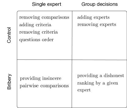
Figure 1: Different types of decision data manipulations

Obviously, this simple diagram cannot describe all possible manipulation models. In particular, it does not take into account the grafter (bribe giver), i.e. the person who orders the ranking to be manipulated, or how the "tampering" is paid. In practice, therefore, in addition to the facilitator and experts, we also need to consider the actual perpetrator, the grafter who benefits from the manipulation. It has an indirect influence on the way the decision-making process is disturbed. For example, they may wish to pay in proportion to the scale of the manipulation committed. The bribe budget may be limited, and they may also accept a certain risk of manipulation being detected, etc. Therefore, when defining the decision-making model that is the subject of manipulation, we must also take into account the grafter and the nature of the relationship with the facilitator and experts.

2.2 From electoral systems to decision-making methods

A grafter can always try to manipulate the decision-making process. In some cases, due to the nature of the decision-making procedure and the type of decision data, it may be difficult. For example, Faliszewski et al. proved that the Llull and Copeland voting systems are resistant to certain types of manipulation [15]. In this case, this resistance is understood in a computational manner, i.e. a resistant system is one in which the manipulation algorithm is NP-hard. Much more often, however, manipulation is possible with the use of less complex and time-consuming procedures. In this case, it is important to define the conditions under which the algorithm has a chance to succeed, i.e. enable the intended manipulation and estimate the cost of the proposed solution. The calculation of the cost of manipulation requires the acceptance of some payment schema where the grafter is the payer and the beneficiaries are those involved in the decision-making process. Manipulation algorithms are often analyzed in the context of electoral systems [45, 23, 20, 1, 36]. In such systems, voters play the role of experts, politicians are the available alternatives, and employees of the election commission play the role of facilitator. The purpose of such a decision-making process is to elect politicians for the next term of office.

Apart from the obvious similarities between the quantitative PC (pairwise comparisons) method and electoral systems (especially the Llull system [7]), there are many significant differences and extensions that the former has. First of all, it is quantitative, i.e. each of the experts determines both the strength of their preferences and indicates which of the two alternatives is better. As with the Llull system (but unlike many other electoral systems), experts provide comparisons for every single pair of options. In the PC method (but not in the electoral system), the concept of inconsistency [27] is used to assess the quality of data. In other words, not all data provided by experts can produce a ranking (some results may be rejected a priori), while each set of electoral votes leads to a result that must be respected by society.

2.3 Algorithms of manipulation

The above differences, both in terms of the general manipulation model (Section 2.1) and the specificity of the PC method (Section 2.2), prompted us to research the problem of manipulation in the quantitative PC method used in AHP. In our model, we use the microbribery mechanism [15]. This means that the size of the bribe depends on the degree of manipulation (here the number of manipulated comparisons). Another limitation that the model must take into account is the inconsistency of the comparison set. This means that the manipulation, in order to be effective, cannot significantly disturb the inconsistency of the set of comparisons.

Based on these assumptions, we defined two heuristic manipulation algorithms. Each of the algorithms tries to propose the smallest possible number of micro-bribes so that the result meets the given level of data consistency. The tests performed prove that the algorithms do not always succeed.

3 Pairwise comparisons

In the PC method, the expert, often referred to as the decision-maker (DM), compares alternatives in pairs. It is convenient to represent the results of the comparisons in the form of an $n\times n$ matrix

$$\boldsymbol{C}=\left[c_{ij}\right],$$ (1)

where $n$ denotes the number of alternatives, and every single element $c_{ij}$ indicates the result of comparison between the $a_{i}$ and $a_{j}$ alternatives. It is natural to expect that if comparing alternative $a_{i}$ to $a_{j}$ makes $c_{ij}$, then the reverse comparison $a_{j}$ to $a_{i}$ gives

$$c_{ij}=\frac{1}{c_{ji}}.$$ (2)

If it is so for every $i,j\in\{1,\ldots,n\}$, then the PC matrix $\boldsymbol{C}$ is said to be reciprocal.

The purpose of the PC method is to calculate a ranking of $n$ alternatives $A=\{a_{1},\ldots,a_{n}\}$ using a PC matrix $C$ as the input. We will write down the calculated ranking value of $a_{i}$ as $w(a_{i})$. The complete ranking takes the form of a priority vector:

$$w^{T}=\left[w(a_{1}),\ldots,w(a_{n})\right]^{T}.$$

Very often it is assumed that the priority vector is rescaled so the sum of its entries equals $1$, i.e. $\sum_{i=1}^{n}w(a_{i})=1$. This assumption enables an easy assessment of the significance of a given alternative without having to consider other priorities.

There are many different ways to compute a priority vector using PC matrices [27]. One of the most popular is the Eigenvalue method (EVM) proposed by Saaty in his seminal work on AHP [34]. In this approach, the priority vector is calculated as an appropriately rescaled principal eigenvector of $C$. Hence, the priority vector $w=\left[w(a_{1}),\ldots,w(a_{n})\right]^{T}$ is calculated as

$$w(a_{i})=\frac{\widehat{w}_{i}}{\sum_{j=1}^{n}\widehat{w}_{j}},$$

where $\widehat{w}$ and $\lambda_{\textit{max}}$ are the principal eigenvector and the principal eigenvalue of $C$ correspondingly, i.e. they satisfy the equation

$$\boldsymbol{C}\widehat{w}=\lambda_{\textit{max}}\widehat{w}.$$ (3)

The second popular priority deriving procedure is the geometric mean method (GMM) [8]. According to this approach, the priority of the i-th alternative is determined by the geometric mean of the i-th row of a PC matrix. Thus, after rescaling, the priority vector is given as $w=\left[w(a_{1}),\ldots,w(a_{n})\right]^{T}$ where

$$w(a_{i})=\frac{\left(\prod_{j=1}^{n}c_{ij}\right)^{1/n}}{\sum_{k=1}^{n}\left(\prod_{j=1}^{n}c_{kj}\right)^{1/n}}.$$

Since elements of $C$ correspond to mutual comparisons of alternatives, one can suppose that they correspond to the ratios formed by the ranking results for individual alternatives, i.e.

$$c_{ij}=\frac{w(a_{i})}{w(a_{j})},\,\,\,\textit{for}\,\,i,j=1,\ldots,n.$$

This entails the expectation of transitivity between the results of comparisons, according to which, for every three alternatives $a_{i},a_{k}$ and $a_{j}$, it holds that

$$\frac{w(a_{i})}{w(a_{k})}\cdot\frac{w(a_{k})}{w(a_{j})}=\frac{w(a_{i})}{w(a_{j})},$$

i.e.,

$$c_{ik}c_{kj}=c_{ij}.$$ (4)

The matrix $C$ where (4) holds is called consistent. Unfortunately, in practice, PC matrices are very often inconsistent. Thus, for some number of alternatives (4) does not hold. This also means that $i,j$ exist for which

$$c_{ij}\neq\frac{w(a_{i})}{w(a_{j})}.$$

In addition to detecting the fact that a given matrix is inconsistent, it is also possible to determine the degree of its inconsistency. For this purpose, inconsistency indices are used [6]. One of the most frequently used indices is the consistency index CI [34] defined as

$$\textit{CI}\left(\boldsymbol{C}\right)=\frac{n-\lambda_{\textit{max}}}{n-1}.$$

In addition to $\textit{CI},$ Saaty introduced the consistency ratio CR defined as

$$\textit{CR}(C)=\frac{\textit{CI}(C)}{\textit{R}(C)},$$

where $\textit{R}(C)$ is the average inconsistency for the fully random PC matrix with the same dimensions as $C$. According to Saaty’s proposal, every PC matrix $C$ for which $\textit{CR}(C)>0.1$ is considered as too inconsistent to be the basis for the ranking. As this threshold was chosen arbitrarily, some researchers question its value [2, 22].

4 Decision model

For the purposes of this study, we assumed that the person performing the manipulation is an expert, and his/her (or grafter’s) goal is such a modification of the given PC matrix that the ranking of the selected alternative $a_{p}$ will become higher than that of the selected alternative $a_{q}$.

Formally speaking, let $r_{C}$ be a function mapping alternatives to their ranking positions calculated using a certain ranking algorithm and the given matrix $C$,

$$r_{C}:\{a_{1},\ldots a_{n}\}\rightarrow\{1,\ldots,n\}.$$

In other words, it holds that $r_{C}(a_{i})<r_{C}(a_{j})$ if and only if $w(a_{i})<w(a_{j})$ for each $i,j\in\{1,\ldots,n\}$, $i\neq j$.

Let $1\leq p<q\leq n$ be selected indices of alternatives. The purpose of the designed algorithms is to transform $C$ into $C^{\prime}$ so that if $r_{C}(a_{p})\leq r_{C}(a_{q})$ then $r_{C^{\prime}}(a_{q})<r_{C^{\prime}}(a_{p})$. The ability to change individual comparisons implies that the expert, and thus the grafter, knows how the “real” set of comparisons should look. They must also be able to communicate with each other to determine how many comparisons can be modified.

According to the adopted micro-bribery strategy, the cost of manipulation depends on the number of changed comparisons. In our model, the cost of changing one comparison is fixed and amounts to 1 unit and does not depend on the size of the change. The adoption of such an assumption prefers a manipulation with the fewest possible number of modified comparisons.

Although in the original AHP the relative strength of preferences is expressed on a fundamental scale, i.e. for a PC matrix $C=[c_{ij}]$ the value $c_{ij}\in\{1/9,1/8,\ldots,1/2,1,2,\ldots,9\}$, we assume that the result of individual comparisons is a positive real number within the range $[1/9,9]$. On the one hand, such an assumption simplifies the reasoning, but on the other does not limit the proposed solution, i.e. the resulting algorithms can be easily extended to use any discrete scale.

The created algorithms must be inconsistency aware. Therefore, they should try to make the inconsistency of the final result less than the value set in advance (in AHP it is commonly assumed that the acceptable inconsistency of $C$ needs to be less than $0.1$, i.e. $\textit{CR}(C)<0.1$ which in most cases also implies that $\textit{CI}(C)<0.1$ [34]).

5 Row algorithm

The first manipulation algorithm is based on the observation that, in general2, increasing $c_{ij}$ causes increasing $w(a_{i})$ at the expense of all other priority values. Thus, providing that our goal is to boost alternative $a_{p}$ so that $r(a_{p})>r(a_{q})$, we will try to increase the subsequent elements in the p-th row of $C$ with inconsistency of the PC matrix in mind.

Assuming that $r$ is monotone, to boost the weight of the i-th alternative let us first try to amplify the i-th row of $C$. Since $r_{C}(a_{p})\leq r_{C}(a_{q})$ then let the first modified element be $c_{pq}$. As $c_{pq}$ is a direct comparison of the pair $(a_{p},a_{q})$ we suppose that it may have the greatest impact on their relative position.

Let $\alpha$ be a positive real number such that $\alpha>\max\{1,c_{pq}\}$. Without the loss of generality, we may assume that $q=1$ and $p=n$ . Thus, in the first step of the algorithm, we update $c_{qp}$ and $c_{pq}$ i.e. $c_{n1}$ and $c_{1n}$ by $\alpha$ and $1/c_{n1}$ correspondingly. Thus, the first approximation of $C$, denoted as $\boldsymbol{C}^{\left(1\right)}$, is given as:

$$\boldsymbol{C}=\boldsymbol{C}^{\left(0\right)}=\begin{bmatrix}1&c_{12}&\cdots&c_{1n}\\ c_{21}&1&&c_{2n}\\ \vdots&&\ddots&\vdots\\ c_{n1}&c_{n2}&\cdots&1\end{bmatrix}^{\left(0\right)}\xrightarrow[1^{\textit{st}}\,\,\textsl{step}]{\textsl{}}$$

$$\xrightarrow[1^{\textit{st}}\,\,\textsl{step}]{\textsl{}}\begin{bmatrix}1&c_{12}&\cdots&1/\alpha\\ c_{21}&1&&c_{2n}\\ \vdots&&\ddots&\vdots\\ \alpha&c_{n2}&\cdots&1\end{bmatrix}^{\left(1\right)}=\boldsymbol{C}^{\left(1\right)}$$

If we find $\alpha$ such that $r_{C^{(1)}}(a_{q})<r_{C^{(1)}}(a_{p})$ then the algorithm stops. Otherwise, we may request further modifications. As

$$c_{pj}=c_{pq}c_{qj}$$ (5)

Hence, assuming that the next element to change is $c_{n2}$, thus $c_{n2}=c_{n1}c_{12}=\alpha c_{12}$. So, the update for the pair $\left(c_{n2},c_{2n}\right)$ is $\left(\alpha c_{12},1/\alpha c_{12}\right)$.

$$\boldsymbol{C}^{\left(1\right)}=\begin{bmatrix}1&c_{12}&\cdots&1/\alpha\\ c_{21}&1&&c_{2n}\\ \vdots&&\ddots&\vdots\\ \alpha&c_{n2}&\cdots&1\end{bmatrix}^{\left(1\right)}\xrightarrow[2^{\textit{nd}}\,\,\textsl{step}]{\textsl{}}$$

$$\xrightarrow[2^{\textit{nd}}\,\,\textsl{step}]{\textsl{}}\begin{bmatrix}1&c_{12}&\cdots&1/\alpha\\ c_{21}&1&&1/\left(\alpha c_{12}\right)\\ \vdots&&\ddots&\vdots\\ \alpha&\alpha c_{12}&\cdots&1\end{bmatrix}^{\left(2\right)}=\boldsymbol{C}^{\left(2\right)}$$

After finishing the algorithm, we may expect that $\boldsymbol{C}^{\left(m\right)}$ contains $m\leq n-1$ altered elements compared to $\boldsymbol{C}^{\left(0\right)}$. It may turn out that $m<n$. In order to determine the moment when the algorithm should be stopped after each step of the calculations, it is necessary to check the condition $r_{C^{\prime}}(a_{q})<r_{C^{\prime}}(a_{p})$. If it is true, we finish the algorithm.

Let us present the above procedure in the form of a structural pseudo-code (Code listing 1).

Function 1 FindM() method

1:function FindM($C$, p, q)

2:     $\alpha$ $\leftarrow$ set to the initial value;

3:     $m^{res}$ $\leftarrow$ $2\cdot n$, where $n$ is a dimension of the matrix $C$

4:     $C^{res}$ $\leftarrow$ $C$

5:     while ($\alpha$ > $1$) do

6:         $m^{temp}$, $C^{temp}$ $\leftarrow$ ComputeChanges($C$, $\alpha$, p, q)

7:         if $(m^{temp}$ < $m^{res})$ then

8:              $m^{res}$ $\leftarrow$ $m^{temp}$

9:              $C^{res}$ $\leftarrow$ $C^{temp}$

10:         else

11:              if $(m^{temp}$ = $m^{res})$ and $(CI(C^{temp})$ $\leq$ $CI(C^{res}))$ then

12:                  $C^{res}$ $\leftarrow$ $C^{temp}$

13:              end if

14:         end if

15:         decrement $\alpha$

16:     end while

17:     return $m^{\textsl{res}}$ and $C^{res}$

18:end function

The heart of the algorithm is the transformation (5). Indeed, we can find it in the code of $\textsl{ComputeChanges}\left(\right)$ (Listing: 2, lines: 30 - 31). In the context of the definition of inconsistency (4), the use of transformation (5) seems to be quite natural. Thus, for the purposes of this paper, we will refer to the approach presented in this section as the row algorithm. The maximal number of main loop (Listing: 2, lines: 26 - 34) iterations is limited by the size of the input matrix $C$, so it is less or equal to $n-2$, and is strictly correlated with the number of modified elements ($n-1$). Taking into consideration the above observations, we could conclude that the row algorithm is useful especially when the input matrix is large, or the computational resources are limited. It is worth noting that this algorithm is also resistant to the inconsistency of the input matrix, because the ComputeChanges() method (Listing: 2) does not need a $\textit{CI}(C)$ value in any of its steps. The number of steps is not associated with the consistency ratio value, it depends only on the $r_{C}$’s comparison result (Listing 1, line: 27). Thus, even an inconsistent matrix will be a valid input for the discussed method.

For the purposes of this study, the row algorithm was written in the form of two functions: FindM() (Listing 1) and ComputeChanges() (Listing 2). FindM() iterates through different $\alpha$’s and chooses the best option proposed by ComputeChanges(), which is responsible for updating elements of $\boldsymbol{C}$. The FindM() function is used in both of the described algorithms and its implementation does not change, unlike the ComputeChanges() function implementation, which is algorithm dependent. The ComputeChanges() (Listing 2) method returns the number of modified elements in the matrix $\boldsymbol{C}$ and modified matrix $\boldsymbol{C}^{\textsl{res}}$. Those values are compared inside the FindM() function and the best solution is selected.

At the beginning, FindM() sets $\alpha$ to the user-defined initial value (Listing 1, 2) not greater than $1$. Then the variables $m^{\textsl{res}}$ and $\boldsymbol{C}^{\textsl{res}}$ are initialized (Listing 1, lines: 3 - 4). Next, the while loop is executed as long as $\alpha$ is greater than $1$ (lines: 5 - 16). The first operation inside while (line: 7) calls the $\textsl{ComputeChanges}\left(\right)$ method (Listing 2), and stores the returned results as $m^{\textsl{temp}}$ and $\boldsymbol{C}^{\textsl{temp}}$. Then, if $\textsl{ComputeChanges}\left(\right)$ alters fewer elements than it did in the previous step (condition in the line: 7) $m^{\textsl{res}}$ and $\boldsymbol{C}^{\textsl{res}}$ are correspondingly updated (lines: 8, 9). If it does not, providing that the number of altered elements in the current and the previous step is the same, and inconsistency of the matrix $\boldsymbol{C}$ decreased, $\boldsymbol{C}^{\textsl{res}}$ is replaced by its more consistent version $\boldsymbol{C}^{\textsl{temp}}$. At the end of the while loop, $\alpha$ is decreased (line: 15). The method ends with returning both: the number of modified elements and the matrix itself (line: 17).

The next part of our row algorithm is contained in $\textsl{ComputeChanges}\left(\right)$ (Listing 2). The method starts with establishing the input parameters for further calculations (lines: 20 - 25). Then the for loop is executed (lines: 26 - 34). It iterates through elements from $row_{p}^{sorted}$ as long as the rank $a_{q}$ is greater than the rank $a_{p}$ (line: 27). Then, we perform the desired update of $c_{\textsl{p}\textsl{j}}^{\textsl{res}}$ and its reciprocal element $c_{jp}^{\textsl{res}}$ (lines: 30 and 31). We also increment the number of modified elements $m^{\textsl{res}}$. $\textsl{ComputeChanges}\left(\right)$ ends up with returning the results: the number of modifications: $m^{\textsl{res}}$ and the modified matrix $\boldsymbol{C}^{\textsl{res}}$ (line: 35). Since, in every turn of the loop only the previously unchanged element can be modified, then since $\boldsymbol{C}^{\textsl{res}}$ is of a finite size $\textsl{ComputeChanges}\left(\right)$ meets the stop condition. For the same reason, the running time of the procedure is $O(n^{2})$.

Function 2 ComputeChanges() method - row algorithm

19:function ComputeChanges($C$, $\alpha$, p, q)

20:     $C^{res}$ $\leftarrow$ $C$

21:     $c^{res}_{pq}$ $\leftarrow$ $\alpha$

22:     $c^{res}_{qp}$ $\leftarrow$ $1/\alpha$

23:     $m^{res}$ $\leftarrow$ $1$

24:     $row_{p}$ $\leftarrow$ get the $p$-th row of $C^{res}$ and remove elements at position $p$ and $q$

25:     $row_{p}^{sorted}$ $\leftarrow$ sort $row_{p}$ elements in ascending order

26:     for each subsequent element $c^{res}_{pj}$ in the $row_{p}^{sorted}$ do

27:         if $r_{C^{res}}(a_{p})>r_{C^{res}}(a_{q})$ then

28:              exit loop

29:         else

30:              $c^{res}_{pj}$ $\leftarrow$ $\alpha\cdot c^{res}_{qj}$

31:              $c^{res}_{jp}$ $\leftarrow$ $1/c^{res}_{pj}$

32:              increment $m^{res}$

33:         end if

34:     end for

35:     return $2\cdot m^{\textsl{res}}$ and $C^{res}$

36:end function

Let us see how the PC matrix changes during the execution of $\textsl{ComputeChanges}\left(\right)$ operation (items changed in each iteration are underlined). Let the change factor $\alpha$ be set to $1.2$.

$$\begin{array}[]{c}\underbrace{\boldsymbol{C}^{\left(0\right)}=\begin{bmatrix}1&0.3203&6.4158&1.5449\\ 3.1224&1&3.2254&1.7171\\ 0.1559&0.3100&1&0.1390\\ 0.6473&0.5824&7.1927&1\end{bmatrix}}\\ \begin{array}[]{cc}w^{\text{$\left(0\right)$}}=\begin{bmatrix}0.2657\\ 0.4242\\ 0.0606\\ 0.2495\end{bmatrix},&\begin{array}[]{ll}\textit{CI}\left(\boldsymbol{C}^{\left(0\right)}\right)&=0.1420\\ \textsl{p}&=3\\ \textsl{q}&=2\end{array}\end{array}\end{array}\xrightarrow[\textsl{iter.}]{\textsl{1st}}$$

$$\xrightarrow[\textsl{iter.}]{\textsl{1st}}\begin{array}[]{c}\underbrace{\boldsymbol{C}^{\left(1\right)}=\begin{bmatrix}1&0.3203&6.4158&1.5449\\ 3.1224&1&\underline{0.8333}&1.7171\\ 0.1559&\underline{1.2000}&1&0.1390\\ 0.6473&0.5824&7.1927&1\end{bmatrix}}\\ \begin{array}[]{cc}w^{\text{$\left(1\right)$}}=\begin{bmatrix}0.2849\\ 0.3332\\ 0.1110\\ 0.2709\end{bmatrix},&\begin{array}[]{ll}\textit{CI}\left(\boldsymbol{C}^{\left(1\right)}\right)&=0.4477\\ r_{C}(a_{\textit{p}})&=1\\ r_{C}(a_{\textit{q}})&=4\end{array}\end{array}\end{array}\xrightarrow[\textsl{iter.}]{\textsl{2nd}}$$

$$\xrightarrow[\textsl{iter.}]{\textsl{2nd}}\begin{array}[]{c}\underbrace{\boldsymbol{C}^{\left(2\right)}=\begin{bmatrix}1&0.3203&6.4158&1.5449\\ 3.1224&1&0.8333&1.7171\\ 0.1559&1.2000&1&\underline{2.0605}\\ 0.6473&0.5824&\underline{0.4853}&1\end{bmatrix}}\\ \begin{array}[]{cc}w^{\text{$\left(2\right)$}}=\begin{bmatrix}0.3482\\ 0.3503\\ 0.1769\\ 0.1246\end{bmatrix},&\begin{array}[]{ll}\textit{CI}\left(\boldsymbol{C}^{\left(2\right)}\right)&=0.3783\\ r_{C}(a_{\textit{p}})&=2\\ r_{C}(a_{\textit{q}})&=4\end{array}\end{array}\end{array}\xrightarrow[\textsl{iter.}]{\textsl{3rd}}$$

$$\xrightarrow[\textsl{iter.}]{\textsl{3rd}}\begin{array}[]{c}\underbrace{\boldsymbol{C}^{\left(3\right)}=\begin{bmatrix}1&0.3203&\underline{0.2669}&1.5449\\ 3.1224&1&0.8333&1.7171\\ \underline{3.7469}&1.2000&1&2.0605\\ 0.6473&0.5824&0.4853&1\end{bmatrix}}\\ \begin{array}[]{cc}w^{\text{$\left(3\right)$}}=\begin{bmatrix}0.1394\\ 0.3235\\ 0.3882\\ 0.1489\end{bmatrix},&\begin{array}[]{ll}\textit{CI}\left(\boldsymbol{C}^{\left(3\right)}\right)&=0.0454\\ r_{C}(a_{\textit{p}})&=4\\ r_{C}(a_{\textit{q}})&=3\end{array}\end{array}\end{array}$$

In each iteration $\textsl{ComputeChanges}\left(\right)$ modifies different elements of $\boldsymbol{C}$. This in turn causes the value of $w$ and consistency of $C$ to change. In the above example, in the third iteration it holds that $r_{C^{\left(3\right)}}(a_{\textit{q}})<r_{C^{\left(3\right)}}(a_{\textit{p}})$. This means the intended goal is reached and the algorithm completed. It is worth noting that the resulting matrix meets the usual consistency criterion i.e. it holds that $\textit{CI}\left(\boldsymbol{C}^{\left(3\right)}\right)\leq 0.1$.

6 Matrix algorithm

In this section, we would like to introduce a slightly different approach to finding appropriate modifications. The priority vector $w$ is directly computed from $\boldsymbol{C}$ (equation 3) and if matrix $\boldsymbol{C}$ is consistent, each $c_{ij}$ element is equal to the ratio of ranking results for $a_{i}$ and $a_{j}$ (equation 4). Hence, the consistent matrix $\boldsymbol{C}^{con}$ can be computed directly from $w$.

Let us also introduce a way to measure the distance between elements of two distinctive matrices $\boldsymbol{A}$ and $\boldsymbol{B}$. The best candidate is a Hadamard product of matrices $\boldsymbol{A}$ and $\boldsymbol{B}^{T}$ defined as:

$$\boldsymbol{H}=[a_{ij}\cdot b_{ji}]=\boldsymbol{A}\bullet\boldsymbol{B}^{T}$$ (6)

which indicates that if $\left|a_{ij}-b_{ij}\right|\thickapprox 0$ then the value of $h_{ij}$ and $h_{ji}$ tends to $1$. It is worth noting that the value of one element is greater than $1$, while the other one is lower.

The main idea of this algorithm is to change elements of matrix $C$ - $c_{ij}$ to its counterparts - $c_{ij}^{con}$ starting from the most distant ones to the closest. Distances are computed using (equation 6), and only the ones which are greater than $1$ are taken into consideration. For the specific element $c_{ij}$ its reciprocal element $c_{ji}$ is also changed. Such a way of choosing and modifying elements leads to the conclusion that the maximal number of modified elements is:

$$m_{max}^{res}=n(n-1)$$ (7)

where $n$ is the size of the matrix $C$. The goal of all algorithms remains the same, making $\textit{rank}_{C^{{}^{\prime}}}(a_{\textit{fp}})\leq\textit{rank}_{C^{{}^{\prime}}}(a_{\textit{ip}})$, so the final value of $m^{res}$ might be lower than $m_{max}^{res}$.

The idea of the matrix algorithm is presented in the listing 3. All of the input parameters are the same as in the row algorithm. In the first step, we initialize local variables (lines: 2, 3) and compute important helper variables (lines: 4-7). To compute $C^{con}$ (line: 5) we use a modified priority vector $w^{\prime}$ which promotes alternative $a_{p}$ over $a_{q}$. Then the for loop is executed (lines: 8-16). It iterates through elements from $respos$ as long as the rank of $a_{q}$ is greater than the rank of $a_{p}$ (line: 9), otherwise the loop is exited (line: 10). Then, we perform the desired update of $c_{ij}^{res}$ (line: 12), its reciprocal element $c_{ji}^{res}$ (line: 13) and we increment $m^{res}$ (line: 14). The described method ends up with returning the number of modified elements - $m^{res}$, and modified matrix $C^{res}$ (line: 17). Since in every turn of the loop previously unchanged elements are modified, after the last possible turn $C^{res}$ is equal to $C^{con}$ and the stop condition is met. For the same reason, the running time of the procedure is $O(n^{2})$.

Function 3 ComputeChanges() method - matrix algorithm

1:function ComputeChanges($C$, $\alpha$, p, q)

2:     $C^{res}$ $\leftarrow$ $C$

3:     $m^{res}$ $\leftarrow$ $0$

4:     $w$ $\leftarrow$ calculate priority vector for matrix $C$

5:     $C^{con}$ $\leftarrow$ generate consistent matrix using vector $w$, where $w_{p}=\alpha w_{q}$

6:     $C^{had}$ $\leftarrow$ calculate Hadamard product for matrix $C$ and matrix ${C^{con}}^{T}$

7:     $respos$ $\leftarrow$ sort $C^{had}$’s elements, greater than one, in descending order

8:     for each subsequent element $c^{had}_{ij}$ in the $respos$ do

9:         if $r_{C^{res}}(a_{p})>r_{C^{res}}(a_{q})$ then

10:              exit loop

11:         else

12:              $c^{res}_{ij}$ $\leftarrow$ $c^{con}_{ij}$

13:              $c^{res}_{ji}$ $\leftarrow$ $c^{con}_{ji}$

14:              increment $m^{res}$

15:         end if

16:     end for

17:     return $2\cdot m^{\textsl{res}}$ and $C^{res}$

18:end function

The workflow of the $\textsl{ComputeChanges}\left(\right)$ method (Listing 3) is presented in the example below. Let the change parameter $\alpha$ be the same as previously i.e. ($\alpha=1.2$). The initial values of $C^{res}$ (Listing 3, line: 2), $C^{had}$ (line: 6) and respos (line: 7) are as follows:

$C^{res}=\begin{bmatrix}1&0.3203&6.4158&1.5449\\ 3.1224&1&3.2254&1.7171\\ 0.1559&0.3100&1&0.1390\\ 0.6473&0.5824&7.1927&1\end{bmatrix}$

$C^{had}=\begin{bmatrix}1&0.51148&12.2943&1.45109\\ 1.95532&1&3.87048&1.00999\\ 0.0813567&0.258333&1&0.0681328\\ 0.689146&0.990145&14.6741&1\end{bmatrix}$

$\textit{respos}=\left\{14.6741,\,12.2943,\,3.87048,\,1.95532,\,1.45109,\,1.00999\right\}$

consecutive steps of the described algorithm are presented below, as well as a detailed description of important variables at each step:

$$\begin{array}[]{c}\underbrace{C^{\left(0\right)}=\begin{bmatrix}1&0.3203&6.4158&1.5449\\ 3.1224&1&3.2254&1.7171\\ 0.1559&0.3100&1&0.1390\\ 0.6473&0.5824&7.1927&1\end{bmatrix}}\\ \begin{array}[]{cc}w^{\text{$\left(0\right)$}}=\begin{bmatrix}0.2657\\ 0.4242\\ 0.0606\\ 0.2495\end{bmatrix},&\begin{array}[]{ll}\textit{CI}\left(\boldsymbol{C}^{\left(0\right)}\right)&=0.1420\\ \textsl{p}&=3\\ \textsl{q}&=2\end{array}\end{array}\end{array}\xrightarrow[\textsl{iter.}]{\textsl{1st}}$$

$$\xrightarrow[\textsl{iter.}]{\textsl{1st}}\begin{array}[]{c}\underbrace{C^{\left(1\right)}=\begin{bmatrix}1&0.3203&6.4158&1.5449\\ 3.1224&1&3.2254&1.7171\\ 0.1559&0.3100&1&\underline{2.0401}\\ 0.6473&0.5824&\underline{0.4902}&1\end{bmatrix}}\\ \begin{array}[]{cc}w^{\text{$\left(1\right)$}}=\begin{bmatrix}0.3084\\ 0.4301\\ 0.1242\\ 0.1374\end{bmatrix},&\begin{array}[]{ll}\textit{CI}\left(\boldsymbol{C}^{\left(1\right)}\right)&=0.2395\\ r_{C}(a_{\textit{p}})&=1\\ r_{C}(a_{\textit{q}})&=4\end{array}\end{array}\end{array}\xrightarrow[\textsl{iter.}]{\textsl{2nd}}$$

$$\xrightarrow[\textsl{iter.}]{\textsl{2nd}}\begin{array}[]{c}\underbrace{C^{\left(2\right)}=\begin{bmatrix}1&0.3203&\underline{0.5219}&1.5449\\ 3.1224&1&3.2254&1.7171\\ \underline{1.9163}&0.3100&1&2.0401\\ 0.6473&0.5824&0.4902&1\end{bmatrix}}\\ \begin{array}[]{cc}w^{\text{$\left(2\right)$}}=\begin{bmatrix}0.1554\\ 0.4626\\ 0.2319\\ 0.1501\end{bmatrix},&\begin{array}[]{ll}\textit{CI}\left(\boldsymbol{C}^{\left(2\right)}\right)&=0.0749\\ r_{C}(a_{\textit{p}})&=3\\ r_{C}(a_{\textit{q}})&=4\end{array}\end{array}\end{array}\xrightarrow[\textsl{iter.}]{\textsl{3rd}}$$

$$\xrightarrow[\textsl{iter.}]{\textsl{3rd}}\begin{array}[]{c}\underbrace{C^{\left(3\right)}=\begin{bmatrix}1&0.3203&0.5219&1.5449\\ 3.1224&1&\underline{0.8333}&1.7171\\ 1.9163&\underline{1.2}&1&2.0401\\ 0.6473&0.5824&0.4902&1\end{bmatrix}}\\ \begin{array}[]{cc}w^{\text{$\left(3\right)$}}=\begin{bmatrix}0.1678\\ 0.3433\\ 0.3364\\ 0.1525\end{bmatrix},&\begin{array}[]{ll}\textit{CI}\left(\boldsymbol{C}^{\left(3\right)}\right)&=0.0351\\ r_{C}(a_{\textit{p}})&=3\\ r_{C}(a_{\textit{q}})&=4\end{array}\end{array}\end{array}\xrightarrow[\textsl{iter.}]{\textsl{4th}}$$

$$\xrightarrow[\textsl{iter.}]{\textsl{4th}}\begin{array}[]{c}\underbrace{C^{\left(4\right)}=\begin{bmatrix}1&\underline{0.6262}&0.5219&1.5449\\ \underline{1.5969}&1&0.8333&1.7171\\ 1.9163&1.2&1&2.0401\\ 0.6473&0.5824&0.4902&1\end{bmatrix}}\\ \begin{array}[]{cc}w^{\text{$\left(4\right)$}}=\begin{bmatrix}0.2013\\ 0.2923\\ 0.3499\\ 0.1565\end{bmatrix},&\begin{array}[]{ll}\textit{CI}\left(\boldsymbol{C}^{\left(4\right)}\right)&=0.0056\\ r_{C}(a_{\textit{p}})&=4\\ r_{C}(a_{\textit{q}})&=3\end{array}\end{array}\end{array}.$$

In each iteration, the PC matrix $C$ elements are modified. Modified elements are underlined to clearly present the workflow of the algorithm. Because it is known in advance how many elements might be modified (equation 7), we might expect that the value of $m^{res}$ is greater than in previously described algorithms (Listing 2). Indeed, the total number of modified matrix $C$ elements is $8$, while “row” algorithms modified only $6$ elements. After execution of the $\textsl{ComputeChanges}\left(\right)$ method (Listing 3) $m^{\textsl{res}}$ and $C^{\textsl{res}}$ are returned inside the slightly modified $\textsl{FindM}\left(\right)$ method (Listing 1). This modification is a change of the initial $m^{res}$ value from $2n$ to $n^{2}$ (line: 3). To find possibly better solutions, the $\textsl{ComputeChanges}\left(\right)$ method might be executed again with different $\alpha$ values.

7 Construction of two algorithms - comparison

The first algorithm (Sec. 5) performs fewer steps and is easier to implement than the second one (Sec. 6). The main advantage of the $\textsl{ComputeChanges}\left(\right)$ method (Listing 2) over its counterpart (Listing 3) is that the number of modified elements in the PC matrix $C$ is limited to $2(n-1)$, where $n$ is the size of $C$, over $\left(n-1\right)^{2}$. The disadvantage of the “row” $\textsl{ComputeChanges}\left(\right)$ method (Listing 2) is it minimizes inconsistency in a slightly chaotic way. Thus, the matrix algorithm’s $\textsl{ComputeChanges}\left(\right)$ (Listing 3) not only gives better results, but it also tries to minimize inconsistency in each step where it is possible. Such a strategy is more effective but, of course, requires more computing power. Both algorithms stop after a finite number of operations are performed. The first $\textsl{ComputeChanges}\left(\right)$ method (Listing 2) has the asymptotic running time of $O(n)$, unlike its counterpart for the matrix algorithm (Listing 3) which has the computational complexity of $O(n^{2})$.

8 Monte Carlo experiments

To verify the proposed algorithms in practice, we conducted a number of Monte Carlo experiments. We paid special attention to the following:

• range of the initial CI in which algorithms give acceptable results

• the number of changes to individual elements needed to perform manipulations

Knowing these two values in practice will allow us to assess the effectiveness of the attack (threat scales) with the use of the proposed heuristics.

For the purposes of the tests, we generate sets of $1000$ inconsistent PC matrices for each CI that fits the range $[0.005k,\,0.005\left(k+1\right)]$, where $k=0,1,2\ldots$. To create a single $n\times n$ inconsistent matrix, we use the disturbance factor $d$. The generation process relies on creating a real random ranking $w$ with values between $1/15$ and $15$. Then, we create the consistent matrix $C$ assuming $c_{ij}=w(a_{i})/w(a_{j})$. To make the matrix inconsistent, we disturb every entry multiplying it by a randomly chosen number from the range $[1/d,\,d]$. If the CR of such a disturbed PC matrix is smaller than some acceptance threshold (the default value is $0.1$) we add that matrix into the testing set $\mathcal{C}^{\textit{in}}$. Otherwise, we keep generating the next matrices until we get $1000$ items in the testing set.

The outcome of the algorithm form a set of result matrices $\mathcal{C}^{\textit{res}}$, i.e. the output (Sec. 5 and 6) is an appropriately manipulated matrix. To be considered correct, it should not be too inconsistent. Therefore, we require the input and the "revised" matrix to have a CI not greater than the commonly accepted $0.1$ [34]. Since both algorithms are heuristic (based on the heuristic of monotonicity of the ranking function), it is possible that the algorithm does not find a satisfactory solution. For the purposes of the Monte Carlo experiments, we will call the ratio of correct (consistent enough) outputs to all considered inputs SR (success rate):

$$\textit{SR}\overset{\textit{df}}{=}\frac{\left|\{C^{\textit{res}}\in\mathcal{C}^{\textit{res}}\,:\,\textit{CI}(C^{\textit{res}})\leq 0.1\}\right|}{\left|\mathcal{C}^{\textit{res}}\right|}.$$

The second important parameter of the experiments is the preferential distance between swapped alternatives. Of course, the bigger it is the more demanding the task, and the more difficult it is to manipulate the input PC matrix. Let $\Delta_{pq}$ denote the distance between the position of $a_{p}$ and $a_{q}$ in the ranking:

$$\varDelta_{pq}\coloneqq\left|r_{C}\left(a_{\textit{q}}\right)-r_{C}\left(a_{\textit{p}}\right)\right|.$$

The figures below present the Monte Carlo experiments showing the relationship between SR and CI for different values of $\Delta_{pq}$.

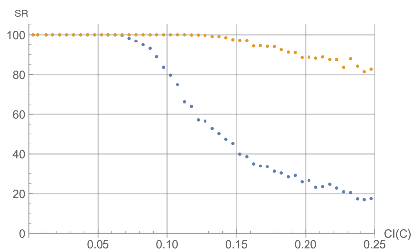
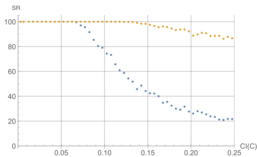
(a) Input matrix of size $n=5$, where $\varDelta_{pq}=1$ and $4$.

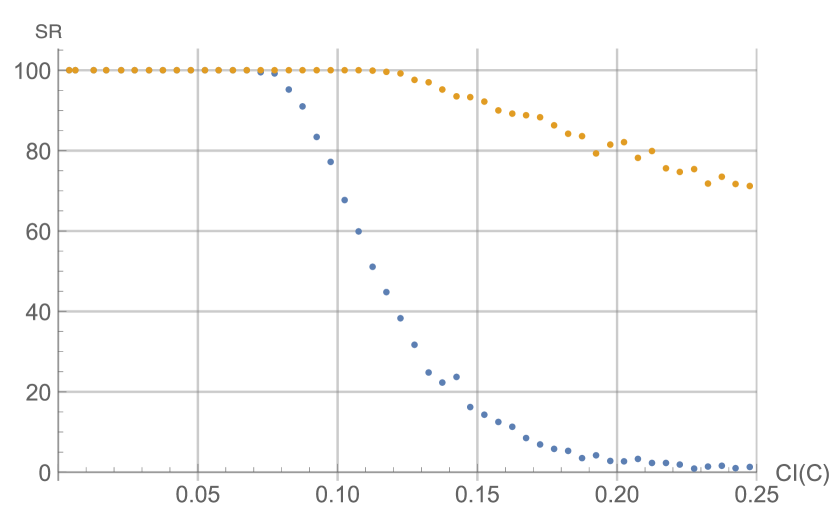
(b) Input matrix of size $n=7$, where $\varDelta_{pq}=1$ and $6$.

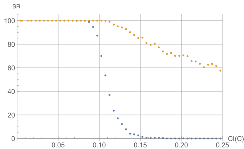
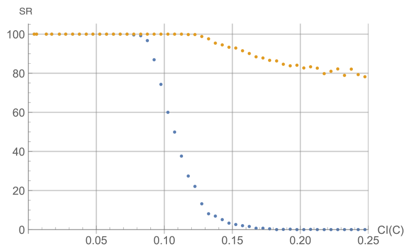
(c) Input matrix of size $n=9$, where $\varDelta_{pq}=1$ and $8$.

row algorithm, matrix algorithm

Figure 2: Success rate for manipulation algorithms with different size of PC matrices and different preferential distance $\Delta_{pq}$.

It is easy to observe that the matrix algorithm performs better than the row algorithm. Indeed, in the case of the former, the SR values decrease more slowly (Figure 2). The matrix algorithm seems to be resistant to changes in the matrix size. The row algorithm is the opposite. The larger the matrix, the more difficult it is to find a sufficiently consistent solution. An interesting effect of the distance $\Delta pq$ on the results can be observed in the case of the matrix algorithm. The greater the distance between alternatives subject to swap seems to be more favorable for it. I.e. in such a case more experiments are successful.

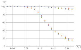
(a) $\varDelta_{pq}=1$

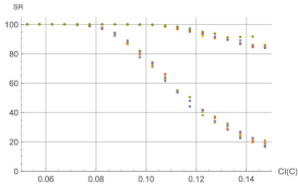
(b) $\varDelta_{pq}=2$

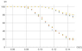
(c) $\varDelta_{pq}=3$

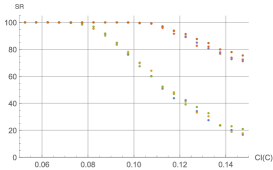
(d) $\varDelta_{pq}=4$

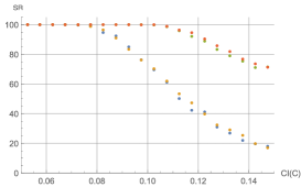
(e) $\varDelta_{pq}=5$

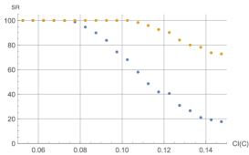
(f) $\varDelta_{pq}=6$

Figure 3: Success rate for $7\times 7$ random PC matrices and different $\varDelta_{pq}$.

The next series of experiments (Fig. 3) suggests that SR does not depend on $\Delta_{pq}$. This result is somewhat surprising, as it means that the preferential distance between the alternatives to be replaced is not a factor decisive for the success of the manipulation.

We test both algorithms against two ranking methods - EVM and GMM. The results are quite similar (Fig. 4), which seems to support the observation that the lack of monotony of the former is not that important in practice and does not affect the operation of algorithms.

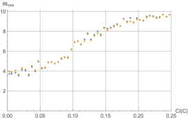
(a) Input matrix of size $n=5$.

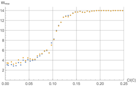
(b) Input matrix of size $n=7$.

EVM, GMM

Figure 4: Number of matrix elements changed using different priority deriving methods: EVM and GMM.

The purpose of the last experiment is to check how many elements are changed by both algorithms.

For each of the $1000$ matrices (for which the inconsistency CI is in range ($[0.005k,\,0.005\left(k+1\right)]$, where $k=0,1,2\ldots$) we execute both algorithms and count the number of elements changed. Then we calculate the average number of modified elements $\overline{m}_{res}$ for each of the intervals. The results are presented below (Fig. 5).

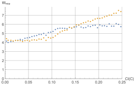
(a) PC matrix of size $n=5$.

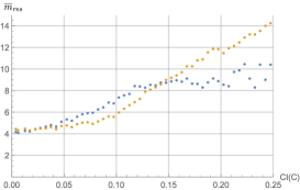
(b) PC matrix of size $n=7$.

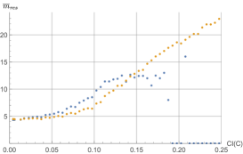
(c) PC matrix of size $n=9$.

Row algorithm, Matrix algorithm

Figure 5: Average number of changed elements $\overline{m}_{res}$ for a matrix with a given inconsistency

9 Discussion

The performed experiments (Sec. 8) show that the algorithms effectively work when some initial conditions for $C$ are met. One of them is the initial inconsistency of the input. Let us look at the charts showing the relationship between the inconsistency CI and the average number of changed elements $\overline{m}_{res}$ and the success rate SR (Fig. 6).

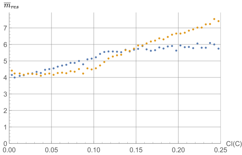
(a) SR and $\overline{m}_{res}$ for PC matrix of size $n=5$

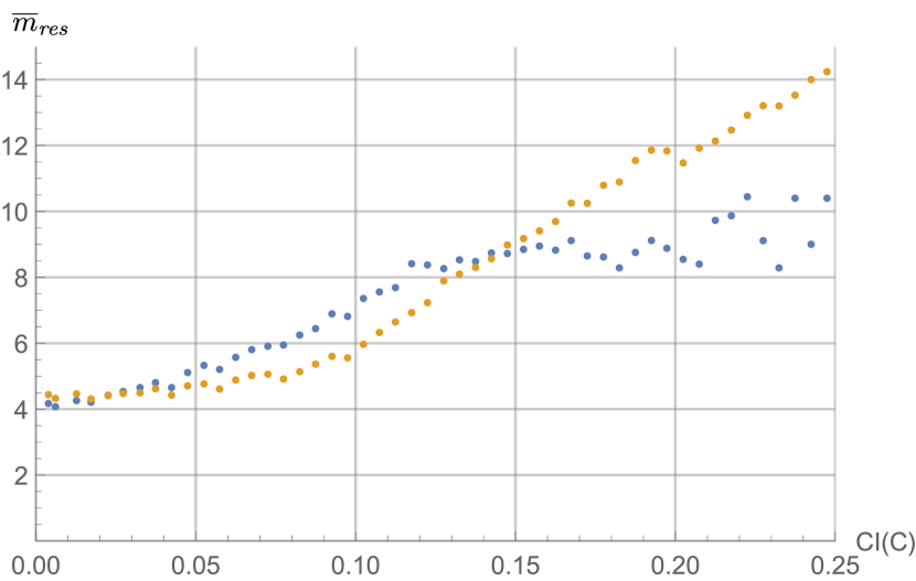
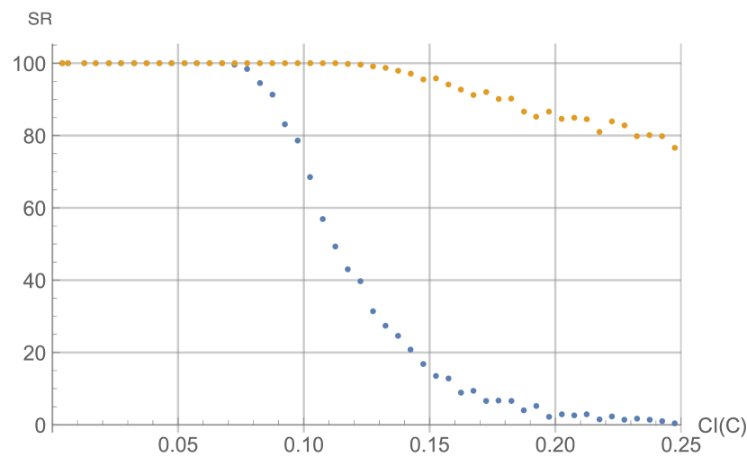
(b) SR and $\overline{m}_{res}$ for PC matrix of size $n=7$

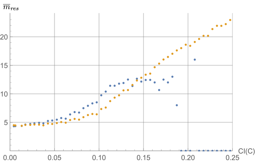
(c) SR and $\overline{m}_{res}$ for PC matrix of size $n=9$

Row algorithm, Matrix algorithm

Figure 6: Comparison of $\overline{m}_{res}$ and SR in relation to the inconsistency index CI.

One may observe that the matrix algorithm modified fewer elements than the row algorithm when inconsistency was not larger than 0.15. At the same time, SR for the matrix algorithm is close to one. The row algorithm performs worse than the matrix one. For inconsistency higher than 0.8, its success ratio visibly drops. This result suggests that the matrix algorithm, albeit a bit more complex, is better than the row approach.

In the context of an algorithmic attack on the decision-making process, a question can be asked about the possibility of its detection. In the case of the row algorithm, following its mode of operation, we would suggest the following detection method:

1. Divide every element in the $i$-th row by its counterpart in the $j$-th row: $\frac{c_{ik}}{c_{jk}}$ for each $i,j,k\in\{1,\ldots,n\}$, $i\neq j$.

2. If any divided elements have the same value $\frac{c_{ik}}{c_{jk}}=\frac{c_{il}}{c_{jl}}>1$, it may mean that the i-th alternative has been artificially promoted using this algorithm.

The method of detecting the use of the matrix algorithm seems to be more complicated and cannot be detected that easily. Detection of the matrix approach will be the subject of research using machine learning methods.

Monte Carlo experiments prove that the manipulation of two alternatives is possible and, in many cases, relatively easy to perform. The necessary condition to attack the pairwise comparisons decision-making process is the a priori knowledge of the correct (non-manipulated) input matrix, so that it is possible to run the manipulation algorithm and enter its results as the final values of the PC matrix. This assumes either access of a grafter to an expert (or experts) during the decision-making process or such organization of the process that the expert has enough time to carry out calculations over the presented solutions. The above consideration leads to the observation that, in the case of the threat of an attack with micro-bribes, the easiest way to protect the decision procedure is to modify the decision-making process to exclude the possibility of third-party interaction with the experts. In addition, it would be worth considering providing experts with appropriate working conditions with not too much and not too little time for individual decisions.

10 Summary

Decision-making methods based on quantitative pairwise comparisons are, unfortunately, prone to manipulation. We proposed the manipulation model and two attack algorithms using the micro-bribes approach in the presented work. Furthermore, we have analyzed their effectiveness and indicated the circumstances they can be effective in. In our considerations, we took into account the issue of data inconsistency. An important issue that challenges researchers is the detection of manipulation. In future research, we intend to focus on this issue, especially in the context of algorithmic manipulations. An important issue that has not been appropriately addressed is manipulation detection. Thus, this matter will be a challenge for us in future research.

Literature

References

- [1] H. Aziz and A. Lam. Obvious manipulability of voting rules. In Dimitris Fotakis and David Ríos Insua, editors, Algorithmic Decision Theory, pages 179–193, Cham, 2021. Springer International Publishing.
- [2] C. A. Bana e Costa and J. Vansnick. A critical analysis of the eigenvalue method used to derive priorities in AHP. European Journal of Operational Research, 187(3):1422–1428, June 2008.
- [3] J. Barzilai and B. Golany. AHP rank reversal, normalization and aggregation rules. INFOR - Information Systems and Operational Research, 32(2):57–64, 1994.
- [4] V. Belton and T. Gear. On a short-coming of saaty’s method of analytic hierarchies. Omega, 11(3):228 – 230, 1983.
- [5] F. Brandt, V. Conitzer, U. Endriss, J. Lang, and A. D. Procaccia, editors. Handbook of Computational Social Choice. Cambridge University Press, March 2016.
- [6] M. Brunelli. A survey of inconsistency indices for pairwise comparisons. International Journal of General Systems, 47(8):751–771, September 2018.
- [7] J. M. Colomer. Ramon Llull: from ‘Ars electionis’ to social choice theory. Social Choice and Welfare, 40(2):317–328, October 2011.
- [8] G. Crawford and C. Williams. The Analysis of Subjective Judgment Matrices. Technical Report R-2572-1-AF, The Rand Corporation, 1985.
- [9] László Csató and Dóra Gréta Petróczy. On the monotonicity of the eigenvector method. European Journal of Operational Research, 2020.
- [10] Y. Dong, Y. Liu, H. Liang, F. Chiclana, and E. Herrera-Viedma. Strategic weight manipulation in multiple attribute decision making. Omega, 75:154–164, 2018.
- [11] Y. Dong, Q. Zha, H. Zhang, G. Kou, H. Fujita, F. Chiclana, and E. Herrera-Viedma. Consensus reaching in social network group decision making: Research paradigms and challenges. Knowledge-Based Systems, 162(July):3–13, 2018.
- [12] J. S. Dyer. Remarks on the analytic hierarchy process. Management Science, 36(3):249–258, 1990.
- [13] M. Ehrgott, J. R. Figueira, and S. Greco, editors. Trends in Multiple Criteria Decision Analysis, volume 142 of International Series in Operations Research & Management Science. Springer US, Boston, MA, 2010.
- [14] P. Faliszewski, E. Hemaspaandra, and L. A. Hemaspaandra. Using complexity to protect elections. Communications of the ACM, 53(11):74–82, 2010.
- [15] P. Faliszewski, E. Hemaspaandra, L. A. Hemaspaandra, and J. Rothe. Llull and Copeland Voting Computationally Resist Bribery and Constructive Control. J. Artif. Intell. Res. (JAIR), 35:275–341, 2009.
- [16] G. T. Fechner. Elements of psychophysics, volume 1. Holt, Rinehart and Winston, New York, 1966.
- [17] M. Fedrizzi, S. Giove, and N. Predella. Rank Reversal in the AHP with Consistent Judgements: A Numerical Study in Single and Group Decision Making. In Soft Computing Applications for Group Decision-making and Consensus Modeling, pages 213–225. Springer, Cham, Cham, 2018.
- [18] Peter Gärdenfors. Manipulation of social choice functions. Journal of Economic Theory, 13(2):217–228, 1976.
- [19] A. Gibbard. Manipulation of Voting Schemes, 1973.
- [20] S. Gupta, P. Jain, F. Panolan, S. Roy, and S. Saurabh. Gerrymandering on graphs: Computational complexity and parameterized algorithms. In Ioannis Caragiannis and Kristoffer Arnsfelt Hansen, editors, Algorithmic Game Theory, pages 140–155, Cham, 2021. Springer International Publishing.
- [21] M. Kadziński, K. Ciomek, and R. Słowiński. Modeling assignment-based pairwise comparisons within integrated framework for value-driven multiple criteria sorting. European Journal of Operational Research, 241(3):830–841, 2015.
- [22] S. Karapetrovic and E. S. Rosenbloom. A quality control approach to consistency paradoxes in AHP. Eur. J. Oper. Res., 119(3):704–718, 1999.
- [23] O. Keller, A. Hassidim, and N. Hazon. New Approximations for Coalitional Manipulation in Scoring Rules. Journal of Artificial Intelligence Research, 64:109–145, January 2019.
- [24] J. S. Kelly. Almost all social choice rules are highly manipulable, but a few aren’t. Social Choice and Welfare, 10(2):161–175, 1993.
- [25] C. Klamler. A comparison of the Dodgson method and the Copeland rule. Economic Bulletin, pages 1–6, January 2003.
- [26] K. Kułakowski. Heuristic Rating Estimation Approach to The Pairwise Comparisons Method. Fundamenta Informaticae, 133:367–386, 2014.
- [27] K. Kułakowski. Understanding the Analytic Hierarchy Process. Chapman and Hall / CRC Press, 2020.
- [28] K. Kułakowski, K. Grobler-Dębska, and J. Wąs. Heuristic rating estimation: geometric approach. Journal of Global Optimization, 62, 2014.
- [29] K. Kułakowski and D. Talaga. Inconsistency indices for incomplete pairwise comparisons matrices. International Journal of General Systems, 49(2):174–200, 2020.
- [30] J. Michnik. Weighted influence non-linear gauge system (WINGS)-An analysis method for the systems of interrelated components. European Journal of Operational Research, 228(3):536–544, 2013.
- [31] D. Pan, X. Liu, J. Liu, and Y. Deng. A Ranking Procedure by Incomplete Pairwise Comparisons Using Information Entropy and Dempster-Shafer Evidence Theory. The Scientific World Journal, pages 1–11, August 2014.
- [32] J. Rezaei. Best-worst multi-criteria decision-making method. Omega, 53(C):49–57, June 2015.
- [33] D. G. Saari and V. R. Merlin. The Copeland method. Economic Theory, 8(1):51–76, February 1996.
- [34] T. L. Saaty. A scaling method for priorities in hierarchical structures. Journal of Mathematical Psychology, 15(3):234 – 281, 1977.
- [35] T. L. Saaty and G. L. Vargas. The legitimacy of rank reversal. Omega, 12(5):513–516, 1984.
- [36] L. Schmerler and N. Hazon. Strategic voting in negotiating teams. In D. Fotakis and D. Ríos Insua, editors, Algorithmic Decision Theory, pages 209–223, Cham, 2021. Springer International Publishing.
- [37] B. Schoner, W. C. Wedley, and E. U. Choo. A unified approach to ahp with linking pins. European Journal of Operational Research, 64(3):384–392, 1993.
- [38] Sheng Li Si, Xiao Yue You, Hu Chen Liu, and Ping Zhang. DEMATEL Technique: A Systematic Review of the State-of-the-Art Literature on Methodologies and Applications. Mathematical Problems in Engineering, 2018(1), 2018.
- [39] D. A. Smith. Manipulability measures of common social choice functions. Social Choice and Welfare, 16(4):639–661, 1999.
- [40] A. D. Taylor. Social Choice and the Mathematics of Manipulation. Outlooks. Cambridge University Press, 2005.
- [41] L. L. Thurstone. The Method of Paired Comparisons for Social Values. Journal of Abnormal and Social Psychology, pages 384–400, 1927.
- [42] L. L. Thurstone. A law of comparative judgment, reprint of an original work published in 1927. Psychological Review, 101:266–270, 1994.
- [43] R. R. Yager. Penalizing strategic preference manipulation in multi-agent decision making. IEEE Transactions on Fuzzy Systems, 9(3):393–403, 2001.
- [44] R. R. Yager. Defending against strategic manipulation in uninorm-based multi-agent decision making. European Journal of Operational Research, 141(1):217–232, 2002.
- [45] M. Zuckerman, A. D. Procaccia, and J. S. Rosenschein. Algorithms for the coalitional manipulation problem. Artificial Intelligence, 173(2):392–412, February 2009.