Leveraging Domain Features for Detecting Adversarial Attacks Against Deep Speech Recognition in Noise
Abstract
In recent years, significant progress has been made in deep model-based automatic speech recognition (ASR), leading to its widespread deployment in the real world. At the same time, adversarial attacks against deep ASR systems are highly successful. Various methods have been proposed to defend ASR systems from these attacks. However, existing classification based methods focus on the design of deep learning models while lacking exploration of domain specific features. This work leverages filter bank-based features to better capture the characteristics of attacks for improved detection. Furthermore, the paper analyses the potentials of using speech and non-speech parts separately in detecting adversarial attacks. In the end, considering adverse environments where ASR systems may be deployed, we study the impact of acoustic noise of various types and signal-to-noise ratios. Extensive experiments show that the inverse filter bank features generally perform better in both clean and noisy environments, the detection is effective using either speech or non-speech part, and the acoustic noise can largely degrade the detection performance.
Index Terms: Adversarial examples, automatic speech recognition, deep learning, filter bank, noise robustness,
1 Introduction
Numerous successful adversarial attack methods on automatic speech recognition (ASR) systems have been proposed [Iter2017, Carlini2018, schonherr_adversarial_2018, Alzantot2018, Cisse2017a, Kreuk2018, Qin2019a, Taori2019a]. They demonstrate that through small optimised perturbations to an input signal, it is possible to fool an ASR system to produce an alternative targeted result, while the perturbations are largely imperceptible for humans. Prevalence of ASR is on the rise, with already rolled out systems as Google Assistant, Amazon Alexa, Samsung Bixby, Apple Siri and Microsoft Cortana. And with them comes an ever increasing attack surface. The aforementioned systems are potentially responsible for home automation, e.g. turning on and off devices, and for administrative tasks, e.g. making purchases online. Adversarial attacks can make a voice assistant behave maliciously and thus cause a significant threat to the security, privacy, and even safety of its user [yan2022survey]. Obviously, without validating the request being legitimate will leave security holes in users systems.
The nature of attacks can be targeted or untargeted. While the goal of untargeted attacks is to force the ASR model to produce an incorrect class, targeted attacks aim to make the model output a predetermined class and thus are most dangerous in terms of intrusive behaviour. In this work, we will focus on targeted attacks only.
Strategies for defending adversarial attacks can be categorised as proactive and reactive [Hu2019]. In proactive defences, one seeks to build more robust ASR models, e.g. through training with adversarial examples. With reactive approaches, one aims to detect the existence of adversarial attacks at testing time. There exist a number of reactive defence methods. The works in [Das2019, rajaratnam_isolated_nodate, subramanian_robustness_2019, rajaratnam2018noise] defend against audio adversarial attacks by preprocessing a speech signal prior to passing it onto the ASR system. An unsupervised method with no need for labelled attacks is presented in [Akinwande2020], where the defence is realised using anomalous pattern detection. Rather than detecting adversarial examples, the work in [yang_characterizing_2019] characterises them using temporal dependencies.
In [samizade_adversarial_2019], adversarial example detection is formulated as a binary classification problem, in which a convolutional neural network (CNN) is used as the model and Mel-frequency cepstral coefficients (MFCCs) are used as the feature. While MFCC is the most commonly used feature for numerous applications, it remains largely uncontested for this particular defence purpose. Our preliminary study shows that attacks exhibit noticeable energy permutation in high frequency regions, where the resolution of MFCCs is by design sacrificed. Furthermore, it is shown in [yu2017spoofing] that cepstral features from learned filter banks that have denser spacing in the high frequency region are more effective in detecting spoofing attacks. We are therefore motivated to contest the MFCC representation with alternative cepstral features that refocus the spectral resolution in different frequency regions.
ASR systems when deployed in the real world will be exposed to adverse acoustic environments. However, detecting adversarial attacks in noise has rarely been investigated in the literature. In this work, we study the impact of acoustic noise on the performance of adversarial attack detection. It is relevant to mention that the success rate of attacking in noisy environments will decrease as briefly shown in [Yuan2018a] and that the noise can change ASR output [rajaratnam2018noise], which is of interest for future study in a systematic way. Furthermore, it is unknown how speech and non-speech parts are useful for adversarial attack detection. This work studies their potentials.
The contribution of this paper is four-fold.
-
•
To our knowledge, this is the first systematic study of various cepstral features for adversarial attack detection and of impact of acoustic noise, speech only, and non-speech only on detection performance. These include MFCC, inverse MFCC (IMFCC), Gammatone frequency cepstral coefficients (GFCC), inverse GFCC (IGFCC) and linear frequency cepstral coefficients (LFCC). These features are not new, but they (except for MFCC) have not been explored for adversarial attack detection. In addition, their use is highly motivated, and significant improvements are obtained using inverse filter banks as in iMFCC and iGFCC. The study of these features further helps understand the characteristics of the adversarial attacks.
-
•
This work systematically studies the impact of adverse environments for the first time and gains much insight.
-
•
The paper analyses the potentials of using speech and non-speech parts separately in detecting attacks.
-
•
A significant effort has been put on making the work reproducible. The source code for reproducing the results with the parameterisation used in this work and a full catalogue of results are made publicly available 111https://aau-es-ml.github.io/adversarial_speech_filterbank_defence/.
The paper is organized as follows. Section II presents background and analysis of audio adversarial attacks. Methodology and experiment design are provided in Section III. Section IV provides experimental results and discussions. The work is concluded in Section V.
2 Background and Analysis
This section presents both white-box and black-box attacks, analyses spectral representations of attacks, and introduces filter banks applied in this work.
2.1 White-box and black-box attacks
This work considers both white-box and black-box attacks. In white-box attacks, the adversary has full access to the parameters of the victim model, while in black-box attacks, the adversary does not have the access to the model parameters. An examples of state-of-the-art white-box attack methods against ASR systems is the gradient-based Carlini & Wagner method [Carlini2018]. An example of black-box attack methods is the gradient-free Alzantot method [Alzantot2018] that uses genetic algorithm optimization. Gradient approximation is used to generate black-box audio adversarial examples in [huang2022generation].
We build our work on the publicly-available adversarial attack data sets provided by our early work in [samizade_adversarial_2019]. For white-box attacks, the Carlini & Wagner method [Carlini2018] is used to attack Baidu DeepSpeech model [battenberg_exploring_2017]. The DeepSpeech model is trained using the publicly available Mozilla Common Voice data set [Mozilla]. For black-box attacks, the Alzantot method [Alzantot2018] is applied to a keyword spotting deep model [sainath_convolutional_nodate] trained with the publicly available Google Speech Command data set [warden2018speech]. All data sets are sampled at 16 kHz.
2.2 Spectral analysis
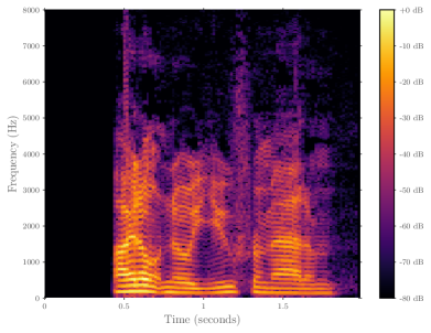
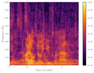
Figure 1 shows the spectrograms of both benign and attacked samples, calculated with a frame length of ms and a frame shift of ms. Inspecting the figure, we hypothesise that for detecting attacks, using filter banks that concentrate resolution in the high frequency regions is beneficial.
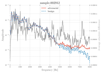
Figure 2 shows an example of the long term average spectrum (LTAS) calculated using Welch’s method [welch1967use] for the benign and adversarial signals, together with the average absolute difference between the two spectra. The difference is computed by taking the spectrograms of both benign and adversarial signals from Fig. 1, subtracting them frame-wise and averaging the absolute residuals. Contrasting the LTAS and the average absolute difference further highlights the importance of high-frequency regions, since the speech signals have much lower energy in high frequency regions and thus perturbations in high frequency regions become relatively more prominent.
2.3 Noisy attack example
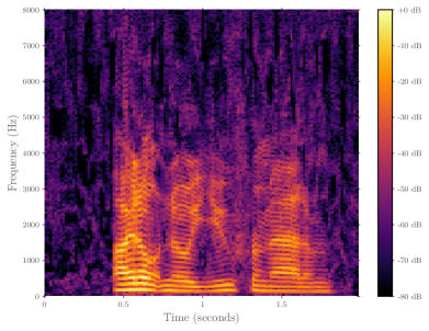
Figure 3 shows two spectra: one for the benign signal and the other for the corresponding attacked signal, both corrupted with babble noise at 10dB SNR. It is clear that the additive noise makes it more difficult to detect attacks.
2.4 Filter banks
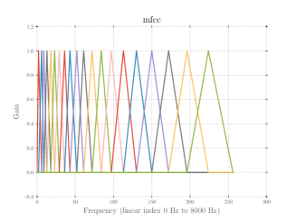
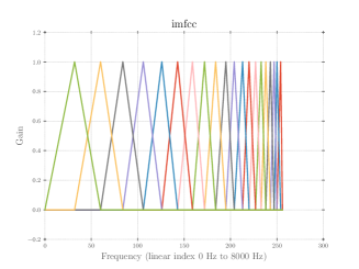
Filter banks are widely used to model the frequency selectivity of an auditory system. Traditionally, the design of filter banks is motivated by psychoacoustic experiments. For example, humans are better at discriminating lower frequencies than higher frequencies, and the Mel-scale triangular filter bank exploits the characteristics of human perception of sound by having higher resolution at lower frequencies than at higher frequencies. Other filter banks are equivalent rectangular bandwidth (ERB) scale Gammatone filter bank and linear triangular filter bank. In this work we also apply the inverse variants of these filter banks. Figure 4 illustrates the regular and inverse variant of the Mel-scale triangular filter banks.
2.4.1 Linear triangular filter bank
In a linear triangular filter bank, the gain of the data point of the triangular band filter is as follows [10.5555/560905]
|
|
(1) |
where is the boundary frequency point of the filter
| (2) |
where is the number of filters, and are the frequency range and is the sampling frequency in Hz.
2.4.2 Mel-scale triangular filter bank
For a Mel-scale triangular filter bank, we construct a triangular filter bank with the boundary frequencies equally spaced on the Mel-scale
|
|
(3) |
where and .
2.4.3 Gammatone filter bank
For a Gammatone filter bank the center frequencies are equally spaced on the equivalent rectangular bandwidth (ERB) scale .
Then the gain of the data point of the the gammatone wavelet filter is computed as
| (4) |
where is the filter order, typically set to , and is the center frequency of the filter
| (5) |
where , and is the number of filters.
2.4.4 Inverse filter banks
Producing the inverse filter bank variant is as simple as reversing the regular filter bank with respect to the frequencies.
3 Methodology and experiment design
3.1 Data sets
The adversarial attack data sets used in this work are from [samizade_adversarial_2019], which are publicly available 222https://github.com/zhenghuatan/Audio-adversarial-examples. We will refer to this article for the specifics on the generation of the adversarial attacks. Data set A (white-box) and data set B (black-box) have and samples, respectively. Data set A contains adversarial samples and benign ones, and Dataset B contains adversarial samples and benign ones, which are reasonably balanced data sets. We conduct extensive experiments using data set A for training and data set B for testing, and vice versa, to investigate the robustness of the proposed methods across types of adversarial attacks.
The data sets provided by [samizade_adversarial_2019] comprise utterances of varying lengths. In order to use a model with inputs of fixed size, we chop the utterances into blocks of ms with a shift of ms, i.e. no overlap. This is in contrast to [samizade_adversarial_2019], where zero-padding is applied to match the longest utterance in the data sets. The issues with zero-padding are that the length of the longest utterance in the data set (rather than the problem domain itself) determines the model size, and computational resources are wasted by adding many zeros. Utterance-level decision can be made easily by later fusion of block level decisions, which is out of the scope of this work.
After block chopping, we split the data into training, validation and test subsets. In order to make the data split unbiased and fully reproducible, we use a hash function-based selection on the utterance filenames, targeting at for training, for validation and for test. In the end, the blocks amount to adversarial attack blocks and benign blocks for training, validation, testing splits from data set A. From data set B we end up with adversarial attack blocks and benign blocks.
3.2 Detection model
We use CNNs to classify an input as either being benign or adversarial. The chosen model architecture and hyperparameterisation mostly follows [samizade_adversarial_2019]. One change is to have a fixed input size as , corresponding to (#frames, #cepstral coefficients), throughout all experiments. Additionally our model has one single output for binary classification. This slightly modified architecture is found in Table 3.2.