Detection of complex nitrogen-bearing molecule ethyl cyanide towards the hot molecular core G10.47+0.03

Abstract

The studies of the complex organic molecular lines towards the hot molecular cores at millimeter and submillimeter wavelengths provide instructive knowledge about the chemical complexity in the interstellar medium (ISM). We present the detection of the rotational emission lines of the complex nitrogen-bearing molecule ethyl cyanide (C₂H₅CN) towards the chemically rich hot molecular core G10.47+0.03 using the Atacama Large Millimeter/Submillimeter Array (ALMA) band 4 observations. The estimated column density of C₂H₅CN towards the G10.47+0.03 is (7.7$\pm$0.5)$\times$10¹⁶ cm^-2 with the high rotational temperature of 352.9$\pm$66.8 K. The estimated fractional abundance of C₂H₅CN with respect to H₂ towards the G10.47+0.03 is 5.70$\times$10^-9. We observe that the estimated fractional abundance of C₂H₅CN is similar to the existing three-phase warm-up chemical modelling abundance of C2H5CN. We also discuss the possible formation mechanism of C₂H₅CN towards the hot molecular cores, and we claim the barrierless and exothermic radical-radical reaction between CH2 and CH2CN is responsible for the production of low abundant of C2H5CN ($\sim$10^-9) in the grain surface of G10.47+0.03.

Keywords ISM: individual objects (G10.47+0.03) – ISM: abundances – ISM: kinematics and dynamics – stars: formation – astrochemistry

1 Introduction

In the ISM, or circumstellar shells, more than 270 interstellar complex and prebiotic molecules are identified at millimeter and submillimeter wavelengths. The identification of the molecular lines from the ISM is a key step in the understanding of the chemical evolution from simple molecular species to molecules of biological relevance (Herbst & van Dishoeck, 2009). The hot molecular cores are known as the early processes of the high-mass star-formation region, which play a key role in increasing the chemical complexity in the ISM (Shimonishi et al., 2021). At this stage, the complex organic molecules are ejected from the icy surfaces of dust grains (Herbst & van Dishoeck, 2009). The hot molecular cores are characterised by their warm temperature ($\gtrsim$100 K), small source size ($\leq$0.1 pc), and high gas density ($\gtrsim$10⁶ cm^-3) (van Dishoeck & Blake, 1998; Kurtz et al., 2000). The time scale of the hot molecular cores lies between $\sim$10⁵ years and $\sim$10⁶ years (van Dishoeck & Blake, 1998; Garrod & Herbst, 2006; Garrod, 2013). The hot molecular cores contain the high-velocity water (H₂O) maser emission, which is located near the ultra-compact (UC) H II regions (Mehringer et al., 2004; Manna & Pal, 2022a). The hot core phase is identified by chemically rich molecular emission spectra with many complex organic molecules, including methyl cyanide (CH₃CN) and methanol (CH₃OH) (Allen et al., 2017). These molecules may be created in the hot molecular cores at a high temperature ($\gtrsim$150 K) via endothermic chemical reactions (Allen et al., 2017). Using high spectral and spatial resolution data like ALMA, VLA, etc., we can identify the different complex organic molecules and the spatial distribution of those complex molecules in the hot molecular cores. The identification of the disk candidates in the hot molecular cores is very rare, which suggests a correlation between disks and hot molecular core chemistry (Allen et al., 2017). The study of the molecular lines in the disk candidate hot molecular cores can help us understand the high-mass star-formation process and chemical evaluation on the small physical scales ($\leq$0.05–0.1 pc) (Allen et al., 2017).

Table 1 : Observation summary of G10.47+0.03.

Observation date On-source time Frequency range Spectral resolution Sensitivity (10 km s^-1) Angular resolution (yyyy-dd-mm) (hh:mm) (GHz) (kHz) (mJy beam^-1) (^′′) 2017-03-05 01:53.40 129.50–130.44 1128.91 0.61 1.67^′′ (14362 au) – – 130.09–130.56  488.28 0.61 – – 130.54–131.01  488.28 0.62 – – 130.50–131.44 1128.91 0.62 2017-01-28 00:33.06 147.50–148.43 1128.91 0.50 1.52^′′ (13072 au) – – 147.55–148.01  488.28 0.50 – – 148.00–148.47  488.28 0.53 – – 148.50–149.43 1128.91 0.53 2017-03-06 01:03.50 153.00–153.93 1128.91 0.66 1.66^′′ (14276 au) – – 153.36–153.83  488.28 0.66 – – 153.82–154.29  488.28 0.67 – – 154.00–154.93 1128.91 0.67 2017-03-07 00:28.72 158.49–159.43 1128.91 0.78 1.76^′′ (15136 au) – – 159.18–159.65  488.28 0.80 – – 159.49–160.43 1128.91 0.79 – – 159.64–160.11  488.28 0.79

The complex organic molecules that contain –C$\equiv$N functional group play a key role in prebiotic chemistry because this functional group is responsible for the formation of peptides, nucleic acids, amino acids, and nucleobases of DNA and RNA in the universe (Balucani, 2009). The complex nitrogen-bearing molecule ethyl cyanide (C₂H₅CN) is also known as propanenitrile, and this is a well-known interstellar molecule which is found in the hot molecular cores and the massive star-formation regions (Mehringer et al., 2004). The dipole moments of the a- and b-conformers of the asymmetric top molecule C₂H₅CN are $\mu_{a}$ = 3.85 D and $\mu_{b}$ = 1.23 D, respectively (Heise et al., 1974). The high dipole moment of C2H5CN indicates that it exhibits a high intensity and dense rotational spectrum. The C2H5CN molecules form on the dust grains of high gas density, the warm inner region of the hot molecular cores (Mehringer et al., 2004). The emission lines of C₂H₅CN were first detected towards the Orion molecular cloud (OMC-1) and Sgr B2, with estimated column densities of 1.8$\times$10¹⁴ cm^-2 and 1.6$\times$10¹⁴ cm^-2, respectively (Johnson et al., 1977). Later, hundreds of the rotational emission lines of C₂H₅CN were detected towards the high-mass star-formation regions Sgr B2, Orion, and W51 (Miao & Snyder, 1997; Liu et al., 2001). The column density of C₂H₅CN towards the Sgr B2 (N) large molecule heimat source or Sgr B2 (N-LMH) hot core reaches 1$\times$10¹⁷ cm^-2 (Miao & Snyder, 1997). The higher-excited transitional lines of C₂H₅CN were also detected in the hot molecular cores Orion KL and Sgr B2 (N) (Daly et al., 2013; Belloche et al., 2013). The vibrationally excited transition lines of C₂H₅CN were also detected in the Sgr B2 and in W51 e2 (Mehringer et al., 2004; Demyk et al., 2008). Earlier, three ¹³C isotopologues of ethyl cyanide, like ¹³CH₃CH₂CN, CH₃¹³CH₂CN, and CH₃CH₂¹³CN were identified in the Orion hot molecular cloud in the frequency ranges of 80–40 GHz and 160–360 GHz (Demyk et al., 2007). The evidence of the C₂H₅CN was also found in the low-mass protostars NGC 1333-IRAS 4A, NGC 1333-IRAS 2A, and IRAS 16293–2422 (Cazaux et al., 2003; Taquet et al., 2015). Recently, evidence of the emission lines of C₂H₅CN was also found in the atmosphere of Titan using the ALMA (Cordiner et al., 2014; Manna & Pal, 2022b).

Table 2 : Summary of the continuum image properties of G10.47+0.03.

Observation date Frequency Integrated flux Peak flux Beam size Position angle RMS (yyyy-dd-mm) (GHz) (Jy) (Jy beam^-1) (^′′$\times$^′′) (^∘) (mJy beam^-1) 2017-03-05 130.234 1.36$\pm$0.01 1.08$\pm$0.08 2.38$\times$1.54 71.35 8.66 130.320 1.31$\pm$0.02 1.02$\pm$0.07 2.36$\times$1.54 72.41 8.50 130.773 1.30$\pm$0.01 1.02$\pm$0.08 2.37$\times$1.52 71.67 5.24 130.949 1.51$\pm$0.03 1.16$\pm$0.08 2.35$\times$1.52 72.15 2.72 2017-01-28 147.692 1.96$\pm$0.03 1.37$\pm$0.01 2.02$\times$1.61 70.06 12.81 147.992 2.06$\pm$0.03 1.44$\pm$0.01 2.01$\times$1.60 69.84 14.20 148.237 2.22$\pm$0.03 1.56$\pm$0.03 2.01$\times$1.60 69.47   9.74 149.044 2.32$\pm$0.03 1.59$\pm$0.01 2.07$\times$1.60 69.73 16.23 2017-03-06 153.486 2.32$\pm$0.02 1.76$\pm$0.02 2.10$\times$1.38 77.92   4.61 153.597 2.11$\pm$0.02 1.62$\pm$0.01 2.11$\times$1.39 77.89   9.08 154.038 2.08$\pm$0.03 1.58$\pm$0.02 2.17$\times$1.39 80.86   9.92 154.482 2.20$\pm$0.02 1.72$\pm$0.04 2.08$\times$1.39 78.13   2.86 2017-03-07 158.942 2.43$\pm$0.03 1.91$\pm$0.01 2.42$\times$1.44 77.48 15.59 159.414 2.39$\pm$0.04 1.87$\pm$0.02 2.46$\times$1.42 75.54   7.67 159.928 2.39$\pm$0.04 1.87$\pm$0.01 2.41$\times$1.45 78.01   5.15 160.155 2.71$\pm$0.05 2.09$\pm$0.02 2.41$\times$1.44 77.74 15.59

The hot molecular core G10.47+0.03 is known as a UC H II region, which is located at a distance of 8.6 kpc with a luminosity of 5$\times$10⁵ L_⊙ (Cesaroni et al., 2010; Sanna et al., 2014). Earlier, the rotational emission lines of complex organic molecules such as methyl isocyanate (CH₃NCO), formamide (NH₂CHO), glycolaldehyde (HOCH₂CHO), methyl isocyanate (HNCO), ethylene glycol ((CH₂OH)₂), methanol (CH₃OH), propanal (CH₃CH₂CHO), acetone (CH₃OCH₃), methyl formate (CH₃OCHO), dimethyl ether (CH₃COCH₃), and acetaldehyde (CH₃CHO) were also found towards the G10.47+0.03 (Rolffs et al., 2011; Gorai et al., 2020; Mondal et al., 2021). The rotational emission lines of possible glycine (NH2CH2COOH) precursor molecules such as methenamine (CH₂NH), methylamine (CH₃NH₂), and amino acetonitrile (NH₂CH₂CN) were also detected from the hot molecular core G10.47+0.03 using the Nobeyama 45 m radio telescope and ALMA band 4 (Suzuki et al., 2016; Ohishi et al., 2019; Manna & Pal, 2022c). Recently, the emission lines of the amide-type molecule cyanamide (NH₂CN) were detected from G10.47+0.03 using the ALMA with an estimated column density of (6.60$\pm$0.1)$\times$10¹⁵ cm^-2 (Manna & Pal, 2022d). The amide-related molecule NH₂CN was previously identified in the ISM as a possible precursor of urea (NH₂CONH₂) (Manna & Pal, 2022d).

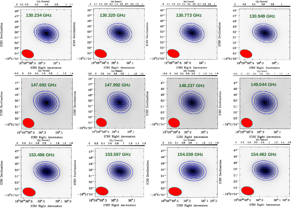
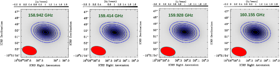
Fig. 1 : Millimeter-wavelength continuum emission images of the hot molecular core G10.47+0.03 obtained with ALMA band 4 in the frequency range 130.234 GHz–160.155 GHz. The contour levels start at 3$\sigma$, where $\sigma$ is the RMS of each continuum image, and the contour levels increase by a factor of $\surd$2. The red circles indicate the synthesised beam of the continuum images. The corresponding synthesised beam size and RMS of all continuum images are presented in Table. 2.

In this article, we present the identification of the rotational emission lines of the complex nitrile-bearing molecule ethyl cyanide (C₂H₅CN) towards the G10.47+0.03 using the ALMA. The observations and data reduction of the raw data of G10.47+0.03 and presented in Section 2. The result of the identification and spatial distribution of C₂H₅CN is shown in Section 3. The discussion and conclusion of the detection of the C₂H₅CN towards G10.47+0.03 are shown in Section 4 and Section 5.

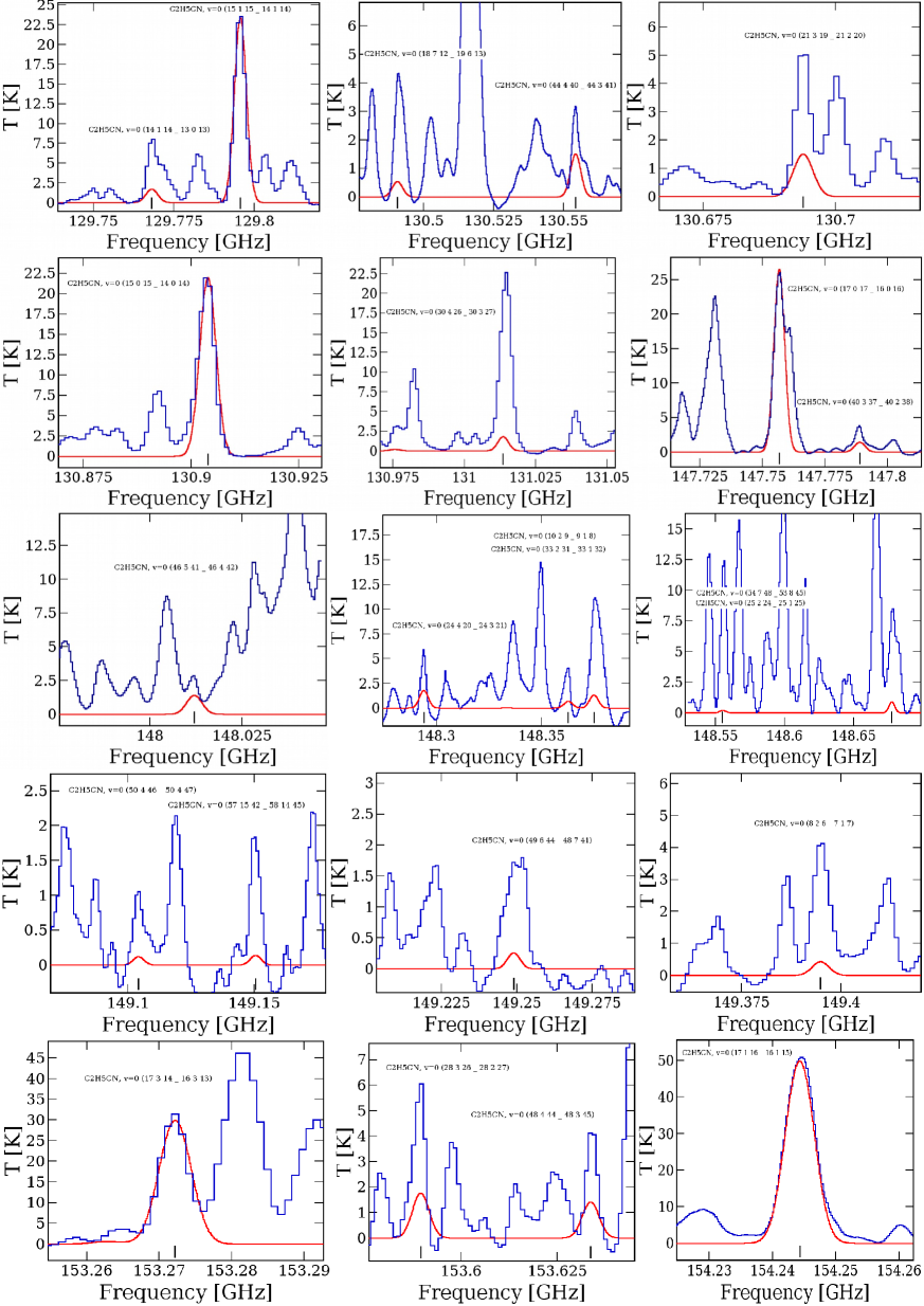
Fig. 2 : Rotational emission lines of C₂H₅CN with different molecular transitions towards the G10.47+0.03 in the frequency ranges of 130.234–130.949 GHz, 147.692–149.044 GHz, 153.486–154.482 GHz, and 158.942–160.155 GHz. The blue spectra indicate the observed millimeter-wavelength molecular spectra of G10.47+0.03, while the red synthetic spectra indicate the best-fitting LTE model over the observed spectra of C₂H₅CN. The black lines indicate the rest frequency positions of the C₂H₅CN transitions.

Figure 2 continued.

Table 3 : Summary of the LTE fitting line properties of the C₂H₅CN towards the G10.47+0.03

Observed frequency Transition $E_{u}$ $A_{ij}$ Gup Optical depth Remark (GHz) (${\rm J^{{}^{\prime}}_{K_{a}^{{}^{\prime}}K_{c}^{{}^{\prime}}}}$–${\rm J^{{}^{\prime\prime}}_{K_{a}^{{}^{\prime\prime}}K_{c}^{{}^{\prime\prime}}}}$) (K) (s^-1) ($\tau$) 129.768 14(1,14)–13(0,13) 44.86 1.33$\times$10^-5 29 7.26$\times$10^-3 Blended with CH3OCH3 129.795 15(1,15)–14(1,14) 51.09 1.82$\times$10^-4 31 1.04$\times$10^-1 Non blended 130.490^∗ 18(7,12)–19(6,13) 127.98 2.17$\times$10^-6 37 1.14$\times$10^-3 Blended with HOCO 130.554 44(4,40)–44(3,41) 448.33 1.47$\times$10^-5 89 6.36$\times$10^-3 Blended with DNO3 130.693 21(3,19)–21(2,20) 109.42 9.84$\times$10^-6 43 6.36$\times$10^-3 Blended with NCHCCO 130.903 15(0,15)–14(0,14) 50.79 1.87$\times$10^-4 31 1.05$\times$10^-1 Non blended 131.013 30(4,26)–30(3,27) 218.54 1.30$\times$10^-5 61 8.22$\times$10^-3 Blended with SO2 147.756 17(0,17)–16(0,16) 64.57 2.69$\times$10^-4 35 1.43$\times$10^-1 Non blended 147.788 40(3,37)–40(2,38) 367.98 1.62$\times$10^-5 81 7.26$\times$10^-3 Blended with CH3COOH 148.012 46(5,41)–46(4,42) 495.98 2.13$\times$10^-5 91 7.13$\times$10^-3 Blended with CH3CDO 148.294 24(4,20)–24(3,21) 147.04 1.63$\times$10^-5 49 9.16$\times$10^-3 Blended with CH3COOH 148.362 10(2,9)–9(1,8) 28.05 9.75$\times$10^-6 21 3.48$\times$10^-3 Blended with CHD2CN 148.374 33(2,31)–33(1,32) 249.49 1.24$\times$10^-5 67 6.78$\times$10^-3 Blended with CH3NCO 148.554 54(7,48)–53(8,45) 694.07 4.77$\times$10^-6 109 1.58$\times$10^-4 Blended with CH3OCHO 148.677 25(2,24)–25(1,25) 143.02 7.74$\times$10^-6 51 4.55$\times$10^-3 Blended with H2CO 149.104 50(4,46)–50(4,47) 573.32 2.20$\times$10^-6 101 6.07$\times$10^-4 Blended with CH3COOH 149.150^∗ 57(15,42)–58(14,45) 959.92 4.09$\times$10^-6 115 3.45$\times$10^-4 Blended with c-C3H2 149.249 49(6,44)–48(7,41) 547.96 4.79$\times$10^-6 99 1.31$\times$10^-3 Blended with HC5N 149.394 8(2,6)–7(1,7) 19.98 7.34$\times$10^-6 17 2.15$\times$10^-3 Blended with CH3COOH 153.272 17(3,14)–16(3,13) 75.97 2.92$\times$10^-4 35 1.39$\times$10^-1 Non blended 153.389 28(3,26)–28(2,27) 184.63 1.44$\times$10^-5 57 7.72$\times$10^-3 Blended with CH3COOH 153.633 48(4,44)–48(3,45) 529.95 2.14$\times$10^-5 97 6.18$\times$10^-3 Blended with CH3COOH 154.244 17(1,16)–16(1,15) 68.17 3.06$\times$10^-4 35 1.47$\times$10^-1 Non blended 154.424 41(12,30)–42(11,31) 529.99 4.29$\times$10^-6 86 1.05$\times$10^-3 Blended with CH3OH 154.476 21(4,17)–21(3,18) 117.24 1.76$\times$10^-5 43 8.83$\times$10^-3 Blended with CHCNH⁺ 154.489 45(5,41)–44(6,38) 474.03 5.07$\times$10^-6 91 1.63$\times$10^-3 Blended with HCOCN 154.557 26(2,25)–26(1,26) 154.02 8.40$\times$10^-6 53 4.59$\times$10^-3 Blended with CH3COOH 158.633 50(6,45)–49(7,42) 589.55 5.73$\times$10^-6 101 1.32$\times$10^-3 Blended with CH3COOH 158.742^∗ 20(8,13)–21(7,14) 161.40 3.73$\times$10^-6 41 2.28$\times$10^-3 Blended with HC5N 159.100 44(4,41)–43(5,38) 444.13 3.99$\times$10^-6 89 1.46$\times$10^-3 Blended with C2H5OH 159.330 17(4,13)–17(3,14) 83.61 1.84$\times$10^-5 35 7.89$\times$10^-3 Blended with CH3COOH 159.558 42(5,37)–42(4,38) 417.78 2.43$\times$10^-5 85 2.98$\times$10^-3 Blended with c-C3HCN 159.785 18(1,18)–17(0,17) 72.24 2.71$\times$10^-5 37 1.27$\times$10^-2 Blended with CH3OCHO 159.888 18(2,17)–17(2,16) 77.61 3.39$\times$10^-4 37 1.55$\times$10^-1 Non blended 159.939^∗ 25(9,17)–26(8,18) 229.71 4.16$\times$10^-6 51 6.52$\times$10^-3 Blended with HC5N 160.050 16(4,12)–16(3,13) 76.29 1.84$\times$10^-5 33 8.56$\times$10^-3 Blended with CH3COOH

${*}$ – Transitions contain double with a frequency difference of less than 100 kHz. The second molecular transition of C2H5CN is not shown.

Table 4 : Estimated emitting regions of C2H5CN towards the G10.47+0.03.

Frequency Transition $E_{up}$ Emitting region (GHz) (${\rm J^{{}^{\prime}}_{K_{a}^{{}^{\prime}}K_{c}^{{}^{\prime}}}}$–${\rm J^{{}^{\prime\prime}}_{K_{a}^{{}^{\prime\prime}}K_{c}^{{}^{\prime\prime}}}}$) (K) [^′′] 129.795 15(1,15)–14(1,14) 51.09 1.52 130.903 15(0,15)–14(0,14) 50.79 1.49 147.756 17(0,17)–16(0,16) 64.57 1.51 153.272 17(3,14)–16(3,13) 75.97 1.54 154.244 17(1,16)–16(1,15) 68.17 1.39 159.888 18(2,17)–17(2,16) 77.61 1.36

2 Observations and data reductions

We have used the cycle 4 archival data of the hot molecular core G10.47+0.03, which was observed using the high-resolution Atacama Large Millimeter/Submillimeter Array (ALMA) (#2016.1.00929.S., PI: Ohishi, Masatoshi). The G10.47+0.03 was located at the observed phase center of ($\alpha,\delta$)_J2000 = 18:08:38.232, –19:51:50.400. The observation of G10.47+0.03 was carried out on 28 January 2017, 5 March 2017, 6 March 2017, and 7 March 2017, using the thirty-nine, forty, forty-one, and thirty-nine antennas, respectively. During the observations, the minimum baseline of the antennas was 15 m, and the maximum baseline of the antennas was 331 m. The observations were made with ALMA-band 4 receivers with spectral ranges of 129.50 GHz–160.43 GHz and a corresponding angular resolution of 1.67^′′–1.76^′′. The corresponding spectral resolutions of the observed data were 1128.91 kHz and 488.28 kHz. The flux calibrator was taken as J1733–1304, the bandpass calibrator was taken as J1924–2914, and the phase calibrator was taken as J1832–2039. The observation details are shown in Table 1.

We use the Common Astronomy Software Application (CASA 5.4.1) for the reduction of the ALMA data (McMullin et al., 2007). We use the Perley-Butler 2017 flux calibrator model to scale the continuum flux density of the flux calibrator using the CASA task SETJY with 5% accuracy (Perley & Butler, 2017). We use the task MSTRANSFORM to split the target data with all rest frequencies after the initial data reduction. After the splitting of the target data, we create the continuum images of G10.47+0.03 in all rest frequencies using CASA task TCLEAN with hogbom deconvolar. Now we perform the continuum subtraction procedure from the UV plane using the task UVCONTSUB. After the continuum subtraction, we use the TCLEAN task with a Briggs weighting robust parameter of 0.5 to make the spectral data cubes of G10.47+0.03. Finally, we apply the IMPBCOR task in CASA for the primary beam pattern correction in the synthesised image. Our data analysis procedure is similar to Manna & Pal (2022c) and Manna & Pal (2022d).

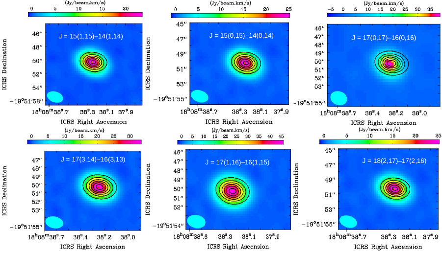
Fig. 3 : Integrated emission maps of non-blended transitions of C₂H₅CN towards the G10.47+0.03. The integrated emission maps of C₂H₅CN are overlaid with the 130.773 GHz (2.29 mm) continuum emission map (black contour). The contour levels start at 3$\sigma$, where $\sigma$ is the RMS of each emission map, and the contour levels increase by a factor of $\surd$2. The cyan circle indicate the synthesised beam of the C₂H₅CN integrated emission maps.

Table 5 : Summary of the Gaussian fitting line properties of the non-blended emission lines of C₂H₅CN towards the G10.47+0.03

Observed frequency Transition $E_{u}$ $A_{ij}$ FWHM $\rm{\int T_{mb}dV}$ (GHz) (${\rm J^{{}^{\prime}}_{K_{a}^{{}^{\prime}}K_{c}^{{}^{\prime}}}}$–${\rm J^{{}^{\prime\prime}}_{K_{a}^{{}^{\prime\prime}}K_{c}^{{}^{\prime\prime}}}}$) (s^-1) (K) (km s^-1) (K km s^-1) 129.795 15(1,15)–14(1,14) 51.09 1.82$\times$10^-4 10.02$\pm$0.69 222.05$\pm$10.24 130.903 15(0,15)–14(0,14) 50.79 1.87$\times$10^-4 10.01$\pm$0.75 193.03$\pm$12.73 147.756 17(0,17)–16(0,16) 64.57 2.69$\times$10^-4 10.81$\pm$0.55 212.83$\pm$22.62 153.272 17(3,14)–16(3,13) 75.97 2.92$\times$10^-4 9.82$\pm$0.87 279.48$\pm$39.65 154.244 17(1,16)–16(1,15) 68.17 3.06$\times$10^-4 10.41$\pm$0.96 342.82$\pm$29.96 159.888 18(2,17)–17(2,16) 77.61 3.39$\times$10^-4 10.29$\pm$0.67 206.34$\pm$35.74

3 Result

3.1 Millimeter wavelength continuum emission towards the G10.47+0.03

We presented the millimeter wavelength continuum emission maps towards the G10.47+0.03 at frequencies of 130.234 GHz, 130.320 GHz, 130.773 GHz, 130.949 GHz, 147.692 GHz, 147.992 GHz, 148.237 GHz, 149.044 GHz, 153.486 GHz, 153.597 GHz, 154.038 GHz, 154.482 GHz, 158.942 GHz, 159.414 GHz, 159.928 GHz, and 160.155 GHz in Figure 1, where the surface brightness colour scale has the unit of Jy beam^-1. We estimate the integrated flux density, peak flux density, synthesised beam size, position angle, and RMS of the G10.47+0.03 to fit a 2D Gaussian over the continuum images using CASA task IMFIT. The estimated continuum image properties of the G10.47+0.03 are shown in Table. 2. After fitting the 2D Gaussian, we observe that the synthesised beam size of the continuum image of G10.47+0.03 is not sufficient to resolve the continua. Previously, Rolffs et al. (2011) detected the submillimeter continuum emission from the G10.47+0.03 in the frequency range of 201–691 GHz with the variation of flux density as 6–95 Jy, corresponding to the spectral index 2.8.

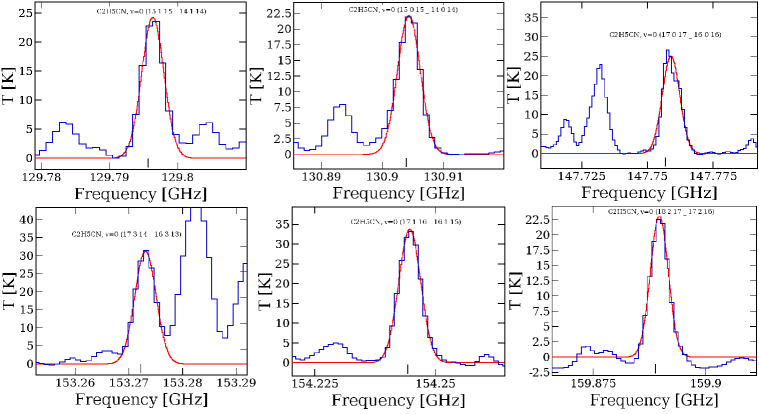
Fig. 4 : Non-blended rotational emission lines of C₂H₅CN with different molecular transitions towards the G10.47+0.03. The blue spectra indicate the observed millimeter-wavelength molecular spectra of G10.47+0.03, while the red synthetic spectra indicate the best-fitting Gaussian model, which was fitted over the non-blended observed spectra of C₂H₅CN. The black lines indicate the rest frequency positions of the C₂H₅CN transitions.

3.2 Identification of C₂H₅CN towards the G10.47+003

We generate the millimeter-wavelength chemically rich spectra from the continuum-subtracted spectral data cubes of G10.47+0.03 to create a circular region with a diameter of 2.5^′′ centred at RA (J2000) = 18^h08^m38^s.232, Dec (J2000) = –19^∘51^′50^′′.440. The systematic velocity ($V_{LSR}$) of the G10.47+0.03 is 68.50 km s^-1 (Rolffs et al., 2011). For identification of the rotational emission lines of C2H5CN towards the G10.47+0.03, we use the local thermodynamic equilibrium (LTE) model with the Cologne Database for Molecular Spectroscopy (CDMS) (Müller et al., 2005) spectroscopic molecular database. We have used the LTE-RADEX module in CASSIS for LTE computing (Vastel et al., 2015). The LTE assumption is valid in the warm inner region of G10.47+0.03 because the gas density of the hot core region of G10.47+0.03 is 7$\times$10⁷ cm^-3 (Rolffs et al., 2011). After the LTE analysis, we detect a total of thirty-six transition lines of C2H5CN within the observable frequency ranges. There are no missing transitions of C2H5CN between the frequency ranges of 130.234–130.949 GHz, 147.692–149.044 GHz, 153.486–154.482 GHz, and 158.942–160.155 GHz. At the full-beam offset position, the best-fit column density of C2H5CN is 8.02$\times$10¹⁶ cm^-2 with excitation temperature 300 K and source size 2.5^′′ (beam size of the data cubes). The FWHM of the LTE model spectra of C2H5CN is 10.2 km s^-1. The LTE-fitted rotational emission lines of C2H5CN are shown in Figure 2.

Recently, Mondal et al. (2023) also analysed the molecular spectra of G10.47+0.03 using the ALMA, and they estimated the column density of C2H5CN to be (1.7$\pm$0.10)$\times$10¹⁷ cm^-2 with an excitation temperature of 150 K. Mondal et al. (2023) fit above the second-order polynomial to reduce the noise level of the spectra, which contributed to the measurement of a higher column density of C2H5CN. Mondal et al. (2023) could not detect all the transition lines of C2H5CN towards the G10.47+0.03 within the observable frequency ranges. Mondal et al. (2023) determined the temperature of C2H5CN using both LTE spectra and a rotational diagram model. There is a discrepancy in the temperature measurement of the C2H5CN emitting region by the two methods used in Mondal et al. (2023). Using LTE modelling, Mondal et al. (2023) estimated the temperature of C2H5CN to be 150 K, which indicates that the molecule is arising from the warm-inner region of the hot core because the temperature of the hot core region of G10.47+0.03 is above 100 K. But, using the rotational diagram method, Mondal et al. (2023) found the temperature of the C2H5CN emitting region to be 92 K, indicating that the molecule is arising from the cold region of the hot core. So, the estimated temperature of C2H5CN by Mondal et al. (2023) is confusing. Earlier, Rolffs et al. (2011) showed that the temperature of C2H5CN emiting region is above 200 K.

After the identification of the rotational emission lines of C2H5CN from the millimeter wavelength spectra of G10.47+0.03, we obtain the molecular transitions (${\rm J^{{}^{\prime}}_{K_{a}^{{}^{\prime}}K_{c}^{{}^{\prime}}}}$–${\rm J^{{}^{\prime\prime}}_{K_{a}^{{}^{\prime\prime}}K_{c}^{{}^{\prime\prime}}}}$), upper state energy ($E_{u}$) in K, Einstein coefficients ($A_{ij}$) in s^-1, $G_{up}$, and optical depth ($\tau$). After the LTE analysis, we observe that J = 15(1,15)–14(1,14), J = 15(0,15)–14(0,14), J = 17(0,17)–16(0,16), J = 17(3,14)–16(3,13), J = 17(1,16)–16(1,15), and J = 18(2,17)–17(2,16) transition lines of C2H5CN are non-blended. We also observe that all non-blended emission lines of C2H5CN are properly fitted with the LTE model, but the blended lines are not properly fitted with the LTE model. The summary of the LTE fitted line properties of C₂H₅CN is shown in Table 3.

3.3 Spatial distribution of C2H5CN

We create the integrated emission maps of non-blended transitions of C₂H₅CN towards the G10.47+0.03. To create the integrated emission maps, we use the task IMMOMENTS in CASA. During the run of the task IMMOMENTS, we define the channel ranges of the data cubes where the emission lines of C₂H₅CN are detected. The integrated emission maps of C₂H₅CN are shown in Figure 3, which are overlaid on the 2.29 mm continuum emission map of G10.47+0.03. After overlaying the continuum emission map over the integrated emission maps of C₂H₅CN, we found that the emission maps of C₂H₅CN have a peak at the position of the continuum. The resultant non-blended integrated emission maps indicate that the different transitions of the C₂H₅CN molecule arise from the highly dense warm inner hot core region of G10.47+0.03. To estimate the emitting regions of C₂H₅CN, we apply the task IMFIT for fitting the 2D Gaussian over the integrated emission maps of C₂H₅CN. The deconvolved synthesised beam size of the C₂H₅CN emitting regions is estimated by the following equation:

$$\theta_{S}=\sqrt{\theta^{2}_{50}-\theta^{2}_{\text{beam}}}$$ (1)

where $\theta_{\text{beam}}$ is the half-power width of the synthesised beam of the C₂H₅CN integrated emission maps and $\theta_{50}=2\sqrt{A/\pi}$ is the diameter of the circle whose area ($A$) is surrounding the $50\%$ line peak of C₂H₅CN (Manna & Pal, 2022c, d). The estimated emitting regions of C₂H₅CN are shown in Table 4. The emitting regions of C₂H₅CN are observed in the range of 1.36^′′–1.54^′′. We notice that the estimated emitting regions of C₂H₅CN are comparable to or slightly greater than the synthesised beam size of the integrated emission maps, which indicates the observed transitions of C₂H₅CN are not well spatially resolved or, at best, marginally resolved. As a result, no conclusions can be drawn about the morphology of the spatial distribution of C2H5CN towards the G10.47+0.03.

3.4 Rotational diagram analysis of C2H5CN

We use the rotational diagram model for the estimation of the column density and rotational temperature of the detected non-blended rotational emission lines of C2H5CN. Initially, we consider that the detected molecular spectra of C2H5CN are optically thin and obey the local thermodynamic equilibrium (LTE) conditions. The LTE approximation is appropriate in the G10.47+0.03 environment because the gas density of the warm inner region of G10.47+0.03 is 7$\times$10⁷ cm^-3 (Rolffs et al., 2011). The column density of the optically thin molecular emission lines can be written as (Goldsmith & Langer, 1999),

$${N_{u}^{thin}}=\frac{3{g_{u}}k_{B}\int{T_{mb}dV}}{8\pi^{3}\nu S\mu^{2}}$$ (2)

where $g_{u}$ indicates the degeneracy of the upper energy ($E_{u}$), $k_{B}$ represents the Boltzmann constant, $\rm{\int T_{mb}dV}$ indicates the integrated intensity, $\mu$ is the electric dipole moment, $S$ denote the strength of the detected molecular emission lines, and $\nu$ is the rest frequency of the identified emission lines of C2H5CN. The equation for total column density under LTE conditions is as follows,

$$\frac{N_{u}^{thin}}{g_{u}}=\frac{N_{\text{total}}}{Q(T_{\text{rot}})}\exp(-E_{u}/k_{B}T_{\text{rot}})$$ (3)

where ${Q(T_{\text{rot}})}$ denotes the partition function as a function of rotational temperature ($T_{\text{rot}}$) and $E_{u}$ denote the identified molecule’s upper energy. The partition functions of C2H5CN at 75 K, 150 K, and 300 K are 4667.9361, 13209.5867, and 37424.5763, respectively. Equation 3 can be rewritten as,

$$ln\left(\frac{N_{u}^{thin}}{g_{u}}\right)=ln\left(\frac{N}{Q}\right)-\left(\frac{E_{u}}{k_{B}T_{rot}}\right)$$ (4)

Equation 4 indicates a linear connection between the values of $\ln(N_{u}/g_{u}$) and E_u of the detected emission lines of C2H5CN. The values $\ln(N_{u}/g_{u}$) are calculated from equation 2. The column density and rotational temperature of C2H5CN can be estimated by fitting a straight line over the values of $ln$(N_u/g_u), which are plotted as a function of E_u. After fitting the straight line, the rotational temperature is estimated from the inverse of the slope, and the column density is estimated from the intercept of the slope. For the rotational diagram, we extract the spectral line parameters of the six non-blended rotational emission lines of C2H5CN using the Gaussian model. We have used the Levenberg-Marquardt (LM) algorithm in CASSIS for fitting the Gaussian model over the detected emission lines of C2H5CN. We observe that the $E_{up}$ of the J = 15(1,15)–14(1,14) and J = 15(0,15)–14(0,14) transition lines of C2H5CN are nearly similar. So, we use only the J = 15(0,15)–14(0,14) transition line for the rotational diagram because the line intensity of J = 15(0,15)–14(0,14) is higher than J = 15(1,15)–14(1,14). The best fit non-blended rotational emission lines of C2H5CN with the Gaussian model is shown in Figure 4 and spectral line fitting parameters are shown in Table 5. To draw the rotational diagram of non-blended transitions of C2H5CN, we use the ROTATIONAL DIAGRAM module in CASSIS. The resultant rotational diagram is shown in Figure 5. In the rotational diagram, the blue error bars represent the error bar of $\ln(N_{u}/g_{u}$), which is calculated from the estimated error of $\rm{\int T_{mb}dV}$ by fitting a Gaussian model over the observed emission lines of C2H5CN. The estimated total column density of C2H5CN towards the G10.47+0.03 is (7.7$\pm$0.5)$\times$10¹⁶ cm^-2 with the high rotational temperature of 352.9$\pm$66.8 K. Our estimated rotational temperature indicate that the emission lines of C2H5CN originated from the hot core region of G10.47+0.03 because Rolffs et al. (2011) claimed the temperature of the hot core of G10.47+0.03 is above 100 K. Our estimated total column density and rotational temperature of C2H5CN are nearly similar to the LTE-fitted column density and excitation temperature of C2H5CN towards the G10.47+0.03. The fractional abundance of C2H5CN with respect to H₂ is calculated to be 5.70$\times$10^-9, and the hydrogen column density towards G10.47+0.03 is calculated to be 1.35$\times$10²⁵ cm^-2 (Gorai et al., 2020).

4 Discussion

4.1 Comparison with observation and modelled abundance of C₂H₅CN

We compare the estimated abundance of C2H5CN with the three-phase warm-up chemical modelling results of Garrod (2013), which is applied in the environment of the hot molecular cores. During the chemical modelling, Garrod (2013) assumed there would be an isothermal collapse phase after a static warm-up phase. In the first phase, the gas density increase from 3$\times$10³ to 10⁷ cm^-3 under the free-fall collapse, and the dust temperature decreases from 16 K to 8 K. In the second phase, the gas density remains constant at $\sim$10⁷ cm^-3 but the dust temperature fluctuates from 8 K to 400 K. The gas density ($n_{H}$) of G10.47+0.03 is 7$\times$10⁷ cm^-3 (Rolffs et al., 2011) and the temperature of the warm region is $\sim$150 K (Rolffs et al., 2011). So, the three-phase warm-up chemical modelling of Garrod (2013), which is applied towards hot molecular cores, is suitable for understanding the chemical evolution of C2H5CN towards G10.47+0.03. In the three-phase warm-up chemical modelling, Garrod (2013) used the fast (5$\times$10⁴–7.12$\times$10⁴ years), medium (2$\times$10⁵–2.85$\times$10⁵ years), and slow (1$\times$10⁶–1.43$\times$10⁶ years) warm-up models based on the time scales. Garrod (2013) estimated the abundance of C2H5CN based on a three-phase warm-up model. After the chemical modelling, Garrod (2013) estimated that the abundance of C2H5CN was 5.7$\times$10^-9 for the fast warm-up model, 7.7$\times$10^-8 for the medium warm-up model, and 3.0$\times$10^-8 for the slow warm-up model. We estimate that the abundance of C2H5CN towards G10.47+0.03 is 5.70$\times$10^-9, which is similar to the simulated abundance of C2H5CN in the fast warm-up model. Earlier, Ohishi et al. (2019), Manna & Pal (2022c), and Manna & Pal (2022d) also claimed that the three-phase warm-up chemical modelling of Garrod (2013) is sufficient to understand the chemical environment of G10.47+0.03.

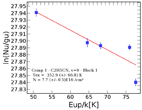
Fig. 5 : Rotational diagram of C2H5CN towards the G10.47+0.03. The blue-filled squares indicate the optically thin approximation data points and blue vertical lines represent the error bars. The best-fit column density and rotational temperature are mentioned inside the image.

4.2 Possible formation mechanism of C₂H₅CN in the hot molecular cores

The complex nitrogen-bearing molecule C2H5CN is produced on the grain surface of the hot molecular cores (Mehringer et al., 2004; Garrod, 2013; Garrod et al., 2017, 2022). In the first stage (the free-fall collapse phase), the peak abundance of C2H5CN is $\sim$10^-9 (Garrod, 2013). In the free-fall collapse stage, the addition of radical CH2 with the radical CH2CN produces the radical CH2CH2CN, and again hydrogenation of the radical CH2CH2CN produces the low abundance of C2H5CN ($\sim$10^-9) on the grain surface of hot molecular cores (Garrod, 2013). The chemical reactions are as follows:

CH2+CH2CN$\rightarrow$CH2CH2CN            (1)

CH2CH2CN+H$\rightarrow$C2H5CN              (2)

Reaction 1 indicates that the addition of radical CH2 and radical CH2CN (alternatively, radical-radical reactions) is barrierless and exothermic (Singh et al., 2021). Our estimated abundance of C2H5CN towards the G10.47+0.03 is 5.70$\times$10^-9, which indicates that reactions 1 and 2 are responsible for the production of the C2H5CN in the grain surface of the G10.47+0.03. Garrod et al. (2017) and Garrod et al. (2022) also used this reaction to simulate the abundance of C2H5CN in the environment of the other hot molecular cores in the free-fall collapse and warm-up phases.

5 Conclusion

We analyse the ALMA band 4 data of the hot molecular core G10.47+0.03 and extract the millimeter wavelength rotational molecular lines. The main conclusions of this work are as follows:

1. We detect a total of thirty-six rotational emission lines of C2H5CN towards the G10.47+0.03 using the ALMA band 4 observation.

2. The estimated column density of C2H5CN towards the G10.47+0.03 is (7.7$\pm$0.5)$\times$10¹⁶ cm^-2 with a rotational temperature of 352.9$\pm$66.8 K. The derived abundance of C2H5CN with respect to H2 towards G10.47+0.03 is 5.70$\times$10^-9.

3. We create the integrated emission maps of non-blended transitions of C2H5CN. From the emission maps, we observe that the non-blended transitions of C2H5CN is arising from the warm-inner region of the G10.47+0.03.

4. We also compare our estimated abundance of C2H5CN with the existing three-phase warm-up chemical modelling abundance of C2H5CN, which is applied towards particularly hot molecular cores. After the comparison, we found that the derived abundance of C2H5CN is nearly similar to the modelled abundance of C2H5CN under the fast warm-up conditions.

5. We also discuss the possible formation mechanism of C2H5CN towards the G10.47+0.03 and we claim the barrierless and exothermic radical-radical reaction between CH2 and CH2CN is responsible for the production of the C2H5CN in the grain surface of G10.47+0.03. The identification of the emission lines of C2H5CN towards the G10.47+0.03 indicates that more complex nitrogen-bearing molecules like propyl cyanide (C3H7CN) are also detectable towards the G10.47+0.03 using the ALMA.

Data availability

The data that support the plots within this paper and other findings of this study are available from the corresponding author upon reasonable request. The raw ALMA data are publicly available at https://almascience.nao.ac.jp/asax/ (project id: 2016.1.00929.S).

Funding

No funds or grants were received during the preparation of this manuscript.

Conflicts of interest

The authors declare no conflict of interest.

Author Contributions

S.P. conceptualize the project. A.M. analysed the ALMA data and identify the emission lines of C2H5CN from the G10.47+0.03. A.M analyses the rotational diagram to derive the column density and rotational temperature of C2H5CN. A.M. and S.P. wrote the main manuscript text. All authors reviewed the manuscript.

References

- Allen et al. (2017) Allen, V., van der Tak, F. F. S., Sánchez-Monge, Á., Cesaroni, R., Beltrán, M. T., 2017, A&A, 603, A133
- Balucani (2009) Balucani N., 2009, Int. J. Mol. Sci, 10, 2304
- Belloche et al. (2013) Belloche, A., Müller, H. S. P., Menten, K. M., Schilke, P., & Comito, C. 2013, A&A, 559, A47
- Cesaroni et al. (2010) Cesaroni, R., Hofner, P., Araya, E., & Kurtz, S. 2010, A&A, 509, A50
- Cordiner et al. (2014) Cordiner, M., Palmer, M., et al. 2014, ApJ, 800, L14
- Cazaux et al. (2003) Cazaux, S., Tielens, A. G. G. M., Ceccarelli, C., et al. 2003, ApJ, 593, L51
- Demyk et al. (2007) Demyk, K., Mder, H., Tercero, B., et al. 2007, A&A, 466, 255
- Demyk et al. (2008) Demyk, K., Wlodarczak, G., & Carvajal, M. 2008, A&A, 489, 589
- Daly et al. (2013) Daly, A. M., Bermdez, C., Lpez, A., et al. 2013, ApJ, 768, 81
- Garrod (2013) Garrod R. T. 2013, ApJS, 765, 60
- Garrod & Herbst (2006) Garrod, R. T., & Herbst, E. 2006, A&A, 457, 927
- Garrod et al. (2017) Garrod, R. T., Belloche, A., Müller, H. S. P., and Menten, K. M., 2017, A&A, 601, A48
- Garrod et al. (2022) Garrod, R. T., Jin, M., Matis, K. A., Jones, D., Willis, E. R., Herbst, E., 2022, ApJS, 259, 1
- Gorai et al. (2020) Gorai, P., Bhat, B., et al. 2020, ApJ, 895 86
- Goldsmith & Langer (1999) Goldsmith, P. F., & Langer, W. D. 1999, ApJ, 517, 209
- Herbst & van Dishoeck (2009) Herbst, E., and van Dishoeck, E. F., 2009, Annu. Rev. Astron. Astrophys, 47, 427
- Heise et al. (1974) Heise, H. M., Lutz, H., & Dreizler, H. 1974, Z. Nat. A, 29a, 1345
- Johnson et al. (1977) Johnson, D. R., Lovas, F. J., Gottlieb, C. A., et al. 1977, ApJ, 218, 370
- Kurtz et al. (2000) Kurtz, S., Cesaroni, R., Churchwell, E., Hofner, P., & Walmsley, C. M. 2000, Protostars and Planets IV, 299
- Liu et al. (2001) Liu, S.-Y., Mehringer, D. M., & Snyder, L. E. 2001, ApJ, 552, 654
- Manna & Pal (2022a) Manna, A. & Pal, S., 2022a, APSS, 367, 94
- Manna & Pal (2022b) Manna, A., & Pal, S., 2022b, Millimeter Wavelength Studies of Complex Nitrile Species in the Atmosphere of Saturn’s Moon Titan, Advances in Modern and Applied Sciences, p.90
- Manna & Pal (2022c) Manna, A. and Pal, S., 2022c, Life Sciences in Space Research, 34, 9
- Manna & Pal (2022d) Manna, A., and Pal, S., 2022d, Journal of Astrophysics and Astronomy, 43, 83
- Mondal et al. (2021) Mondal, S. K., Gorai, P., Sil, M., Ghosh, R., Etim, E. E., Chakrabarti, S. K., Shimonishi, T., Nakatani, N., Furuya, K., Tan, J. C., Das, A., 2021, ApJ, 922(2), p.194
- Mondal et al. (2023) Mondal, S. K., Iqbal, W., Gorai, P., Bhat, B., Wakelam, V., Das, A. 2023, A&A, 669, A71
- Müller et al. (2005) Müller, H. S. P., SchlMder, F., Stutzki, J. & Winnewisser, G. 2005, Journal of Molecular Structure, 742, 215–227
- McMullin et al. (2007) McMullin, J. P., Waters, B., Schiebel, D., Young, W., & Golap, K. 2007, in Astronomical Society of the Pacific Conference Series, Vol. 376, Astronomical Data Analysis Software and Systems XVI, ed. R. A. Shaw, F. Hill, & D. J. Bell, 127
- Mehringer et al. (2004) Mehringer, D. M., Pearson, J. C., Keene, J., & Phillips, T. G. 2004, ApJ, 608, 306
- Miao & Snyder (1997) Miao, Y., & Snyder, L. E. 1997, ApJ, 480, L67
- Ohishi et al. (2019) Ohishi, M., Suzuki, T., Hirota, T., Saito, M. & Kaifu, N. 2019, PASJ, 71
- Perley & Butler (2017) Perley, R. A., Butler, B. J. 2017, ApJ, 230, 1538
- Rolffs et al. (2011) Rolffs, R., Schilke, P., Zhang, Q., & Zapata, L. 2011, A&A, 536, A33
- Sanna et al. (2014) Sanna, A., Reid, M. J., Menten, K. M., et al. 2014, ApJ, 781, 108
- Suzuki et al. (2016) Suzuki, T., Ohishi, M., Hirota, T., Saito, M., Majumdar, L., Wakelam, V., 2016, ApJ, 825, 79
- Shimonishi et al. (2021) Shimonishi, T., Izumi, N., Furuya, K., & Yasui, C., 2021, ApJ, 2, 206
- Singh et al. (2021) Singh, K. K. Tandon, P., Misra, A., Shivani, Yadav, M., Ahmad, A. 2021, International Journal of Astrobiology, 20, 62
- Taquet et al. (2015) Taquet, V., Lpez-Sepulcre, A., Ceccarelli, C., et al. 2015, ApJ, 804, 81
- Vastel et al. (2015) Vastel, C., Bottinelli, S., Caux, E., Glorian, J. -M., Boiziot, M., 2015, Proceedings of the Annual meeting of the French Society of Astronomy and Astrophysics, 313-316
- van Dishoeck & Blake (1998) van Dishoeck, E. F., & Blake, G. A. 1998, Annu. Rev. Astron. Astrophys, 36, 317