nerf2nerf: Pairwise Registration of Neural Radiance Fields

Abstract

We introduce a technique for pairwise registration of neural fields that extends classical optimization-based local registration (i.e. ICP) to operate on Neural Radiance Fields (NeRF) – neural 3D scene representations trained from collections of calibrated images. NeRF does not decompose illumination and color, so to make registration invariant to illumination, we introduce the concept of a “surface field” – a field distilled from a pre-trained NeRF model that measures the likelihood of a point being on the surface of an object. We then cast nerf2nerf registration as a robust optimization that iteratively seeks a rigid transformation that aligns the surface fields of the two scenes. We evaluate the effectiveness of our technique by introducing a dataset of pre-trained NeRF scenes – our synthetic scenes enable quantitative evaluations and comparisons to classical registration techniques, while our real scenes demonstrate the validity of our technique in real-world scenarios. Additional results available at: https://nerf2nerf.github.io

I Introduction

Pairwise registration of 3D scenes that have been acquired in-the-wild is an essential first step in many computer vision and robotic pipelines such as localization [1, 2], pose estimation [3, 4] and large scene reconstruction [5, 6]. Registering 3D scenes that have been acquired in-the-wild presents a number of technical challenges, including noise, outliers, and, most importantly, partial overlap [7, 8].

Acquisition of a 3D scene has classically been achieved via photogrammetry [9], SLAM [10], or depth-fusion [11], where the acquired scene is then represented either in explicit (i.e. a point cloud [9] its reconstructed mesh [12]) or implicit form (i.e. a truncated signed distance function [13]). Recent work has highlighted how these classical 3D reconstruction pipelines struggle in accurately representing many 3D objects [14, Fig. 2], which is problematic if we rely on them as a vehicle for 3D model-based perception in performing robotics tasks.

However, the recent proliferation of research in neural fields [15] coupled with the rapid progression of differentiable rendering [16], has created a new class of 3D representations that leverage volume rendering [17] to relate the underlying 3D substrate to 2D image observations in a differentiable fashion [18, 19, 20]. Among these, Neural Radiance Fields (NeRF) [19] has very rapidly found application in a variety of computer vision applications, and its adoption in robotics has also commenced [21, 22, 14].

Within less than two years, training time for NeRF models was reduced from days [19] to seconds [23], and it is not unreasonable to expect that real-time training from streaming video is within reach. Given these capabilities, one is left to wonder how some of the fundamental tools from 3D geometry processing could be adapted without relying on conversion (e.g. NeRF to polygonal mesh) and classical tools (e.g. polygonal mesh processing). Within this context, in this paper we consider these fundamental questions:

1. “How can a geometric 3D representation be extracted from a pre-trained NeRF?”  such a representation should measure the likelihood of a point in space to lie on the surface of an object – we introduce the concept of “surface fields” as a drop-in replacement for point clouds and polygonal meshes.

2. “How can two scenes acquired under different illumination be registered?”  one cannot rely on radiance comparisons to register two scenes, as view-dependent radiance is the compound effect of material (SVBRDF) and environment lighting – we exploit surface fields and their invariance to illumination.

3. “How can we register two neural fields?”  while fields as Eulerian in nature, most robust registration algorithms assume a Lagrangian representation – we introduce, to the best of our knowledge, the first registration technique that achieves this without relying on implicit-to-explicit conversions.

To validate our findings, we introduce a dataset consisting of scenes with partial overlap – of objects in common between different scenes, and multiple partial observations of an object. The dataset includes synthetic scenes (for quantitative evaluation) as well real-world scenes (for qualitative evaluation and to verify applicability to in-the-wild settings). We evaluate our nerf2nerf algorithm on this dataset, and compare its performance to pipelines relying on conversion to classical representations.

II Related work

Classical registration methods between two 3D point clouds can be split into local and global approaches.  Local methods are typically a variant of the popular Iterative Closest Points (ICP) [24] algorithm – a method that performs registration by optimizing for zero-length closest-point correspondences. However, if it is not carefully initialized, ICP registration is known to converge to local minima [25, 26, 27, 28]. This makes registration of partially overlapping point clouds particularly challenging, as closest-point correspondences can be incorrect even when two partially overlapping scenes are in perfect alignment; this is typically resolved by replacing the least-squares norm with a robust kernel, leading to robust ICP variants [7, 29, 30, 31]. Our solution implements these ideas, but operates on neural fields rather than point clouds, and is capable of registering two pre-trained NeRF models even when they only exhibit partial overlap.  Global methods do not rely on a properly initialized local optimization. For example, fast global registration (FGR) [32] combines the aforementioned robust optimization with feature matching to register point clouds in partial overlap. Other global methods such as [33, 34, 35, 36], compare tuples of points between the two point clouds and optimize for transformations via stochastic search. Recently, neural networks that operate on point clouds [37, 38] have led to new registration techniques that use deep features for correspondence matching [39, 40, 41, 42].

Registration in NeRF

Registration for NeRFs has mostly been explored from the point of view of camera pose estimation. Such works propose to train a NeRF from a collection of images with noisy/unknown pose and jointly optimize for registration and reconstruction [43, 44, 45]. The pioneering work iNeRF [22] predicts, via optimization, the camera pose corresponding to an image of the object for which a pre-trained NeRF model is available. In other words, iNeRF performs image2nerf registration, while we perform nerf2nerf registration. Further, while previous methods perform registration by optimizing with losses based on radiance, we solely leverage radiance to extract a geometric representation from each scene. Consequently, as nerf2nerf relies on the geometry information within the scene, it can register scenes even when there is a mismatch in light configuration.

II-A Neural Radiance Fields

Neural Radiance Fields [46] (NeRFs) are implicit volumetric representations which encode the appearance and geometry of 3D scenes. A NeRF model $\mathcal{R}$ stores a continuous representation of a 3D scene within the parameters $\boldsymbol{\theta}$. It can be seen as a function that maps a position $\mathbf{x}$ in the scene and the viewing direction $\mathbf{d}$ to a view-dependent radiance $\mathbf{c}$ and view-independent density $\tau$:

$$\mathbf{c}(\mathbf{x},\mathbf{d}),\>\tau(\mathbf{x})=\mathcal{R}(\mathbf{x},\mathbf{d};\boldsymbol{\theta})$$ (1)

Given a ray $\mathbf{r}{=}(\mathbf{o},\mathbf{d})$ with origin $\mathbf{o}$ oriented as $\mathbf{d}$, from which a point can be taken at depth $t$ as $\mathbf{r}(t){=}\mathbf{o}{+}t\mathbf{d}$, volume rendering of the radiance field $\mathbf{c}(\mathbf{x},\mathbf{d})$ is computed as:

$$\boldsymbol{C}(\mathbf{r}) =\int_{0}^{t}\mathcal{T}(t;\mathbf{r})\cdot\tau(\mathbf{r}(t))\cdot\mathbf{c}(\mathbf{r}(t),\mathbf{d})\,dt$$ (2)

$$\mathcal{T}(t;\mathbf{r}) =\exp\left(-\int_{0}^{t}\tau(\mathbf{r}(s))\,ds\right)$$ (3)

where $\tau(\mathbf{x})$ is the volumetric density (or extinction coefficient, the differential probability of a viewing ray hitting a particle), and $\mathcal{T}(t;\mathbf{r})$ is the transmittance (or transparency, the probability that the viewing ray travels a distance $t$ along $\mathbf{r}$ without hitting any particle); see [17]. The network parameters $\theta$ of $\mathbf{c}$ and $\tau$ are optimized to minimize the squared distance between the predicted color $\boldsymbol{C}(\mathbf{r})$ and ground truth $\boldsymbol{C}^{\text{gt}}$ for each ray $\mathbf{r}$ sampled from image $\mathbf{I}$:

$$\mathcal{L}_{\text{rgb}}(\boldsymbol{\theta})=\sum_{i}\mathbb{E}_{\mathbf{r}\sim\mathbf{I}_{i}}\left[\|\boldsymbol{C}(\mathbf{r})-\boldsymbol{C}^{\text{gt}}_{i}(\mathbf{r})\|_{2}^{2}\right]$$ (4)

III Method

We are given two 3D scenes represented as (neural) radiance fields, containing a shared substructure $\mathcal{X}$ (e.g. a common object); see Figure 1. We seek a transformation $\mathbf{T}{\in}\text{SE}(3)$ that aligns some shared substructure of the two scenes. Using the notation from Section II-A, these scenes can be represented as radiance fields $\mathcal{R}$:

$$\begin{split}\tau_{a}(\mathbf{x}),\mathbf{c}_{a}(\mathbf{x},\mathbf{d})&=\mathcal{R}_{a}(\mathbf{x},\mathbf{d}),\quad\mathbf{x}{\in}\mathcal{B}(\mathbf{0},r_{a}),\,\mathbf{d}{\in}\mathcal{D}\\ \tau_{b}(\mathbf{x}),\mathbf{c}_{b}(\mathbf{x},\mathbf{d})&=\mathcal{R}_{b}(\mathbf{x},\mathbf{d}),\quad\mathbf{x}{\in}\mathcal{B}(\mathbf{0},r_{b}),\,\mathbf{d}{\in}\mathcal{D}\end{split}$$ (5)

where $\mathcal{B}(\mathbf{0},r)$ is a Euclidean ball of size $r$ centered at the origin, and $\mathcal{D}$ is the subset of unit vectors in ³. Note that, without loss of generality, we assume the fields to be of the same scale and have a bounded domain of radius $r$, centered at the origin. We make no further assumptions about two scenes, such as knowing the extent of the shared substructure, or identical illumination configuration. Our technique only assumes we have access to $\mathcal{R}_{a}$ and $\mathcal{R}_{b}$ during optimization (i.e. the images used to train the NeRF are not available). We formulate the Neural Field registration problem as iterative optimization of a two-term energy:

$$\operatorname*{arg\,min}_{\mathbf{T}}\>\>(1-\lambda^{(t)})\cdot \mathcal{L}_{\text{match}}(\mathcal{S}_{a},\mathcal{S}_{b};\mathbf{T})$$ (Section III-B) (6)

$$+\leavevmode\nobreak\ \lambda^{(t)}\cdot \mathcal{L}_{\text{key}}(\mathcal{Q}_{a},\mathcal{Q}_{b};\mathbf{T})$$ (Section III-C)

where the term $\mathcal{L}_{\text{match}}$ (robustly) measures the distance between two fields given the candidate transformation $\mathbf{T}$, and $\mathcal{L}_{\text{key}}$ measures the distance between two sets of $K$ user-annotated keypoints $\mathcal{Q}{\in}^{K\times 3}$. As the registration computed from keypoints alone is typically noisy (see Figure 1), the term $\lambda$ anneals the optimization over the $T{=}10000$ iterations with an additive trigonometric scheduler, hence gradually shifting the optimization from registering keypoints with $\mathcal{L}_{\text{key}}$ to registering the fields via $\mathcal{L}_{\text{match}}$:

$$\lambda^{(t)}=\tfrac{1}{2}\left(1+\cos{\left(\tfrac{t\pi}{T}\right)}\right).$$ (7)

Light-invariant registration

As we do not assume the light configuration to be identical across the scenes, we cannot compare the radiance terms in (5) to determine whether two scenes are well aligned. Furthermore, working with radiance would require comparisons of distributions over $\mathcal{D}$, as radiance is a view-dependent field. In other words, we employ NeRF and its radiance formulation to generate a sufficiently accurate 3D representation of the geometry within the scene. Geometry, which in a NeRF model is related to the density field $\tau$, is, as desired, lighting invariant. However, as the values of $\tau$ in unobserved areas are not meaningful, in Section III-A we introduce the notion of surface field, the likelihood of a position in space to lie on the surface of a solid object, and describe how they can be distilled from the density field of a NeRF model.

Sample-efficient optimization

While in classical registration pipelines [47] putative correspondences are computed via closest-point [7] or projective [11] correspondences, neural fields do not support this mode of operation (i.e. they are not Lagrangian representations, but Eulerian). One could densely sample $\mathbf{x}\in\mathcal{B}(\mathbf{0},r)$, but this amounts to evaluating the neural model at a very large set of spatial locations. This is not only computationally expensive, but also pointless, as most of these evaluations will be discarded by the robust kernels implementing $\mathcal{L}_{\text{match}}$. To overcome this problem, we introduce a sampling mechanism based on Metropolis-Hastings sampling; see Section III-D.

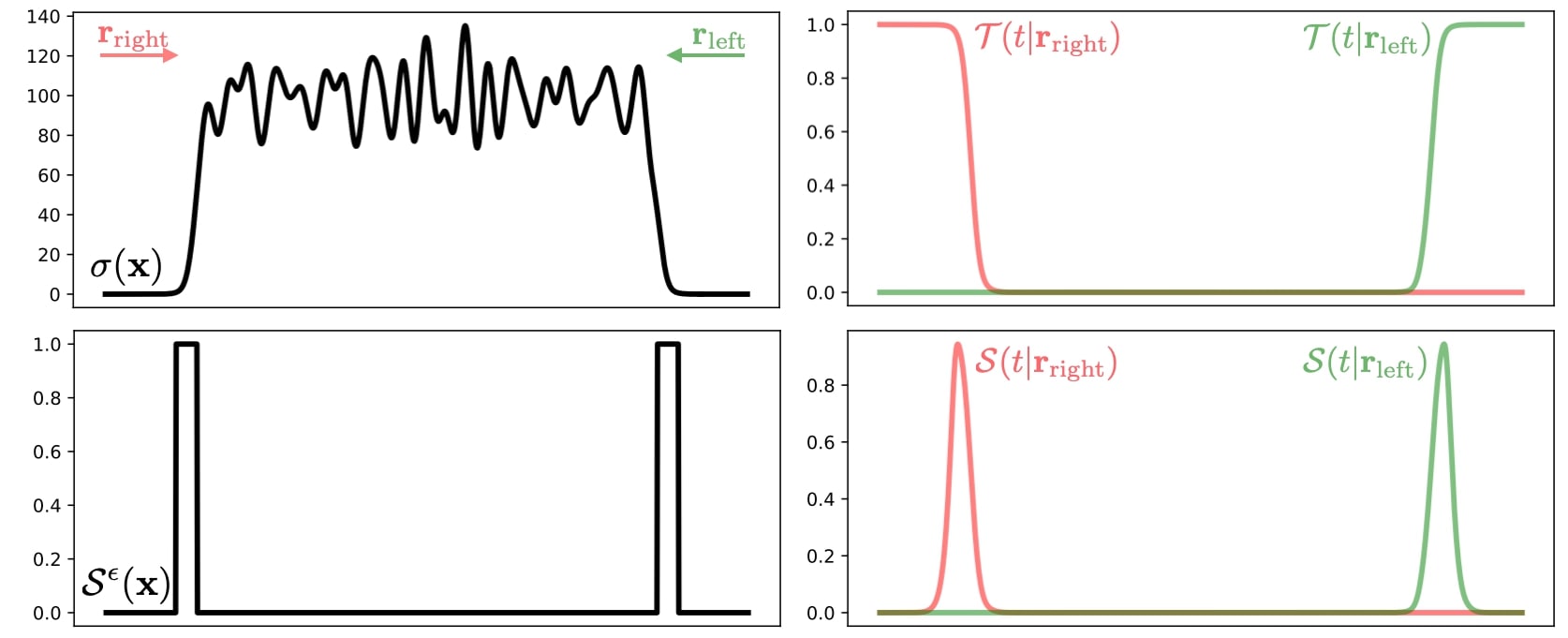
\begin{overpic}[width=429.28616pt]{fig/surfacefield} \put(6.0,-2.5){Color Image} \put(39.0,-2.5){Density Field} \put(72.0,-2.5){Surface Field} \end{overpic}

Figure 2: Surface field – (top) We illustrate the NeRF-like density model for a 2D example of a “rect“ function observed by two rays: one observing the scene from the left, the other from the right. NeRF does not supervise density in areas of occlusion, leading to a null-space that often results in a noisy density function. Transmittance integrates this noise out by modeling occlusion, and our definition of surface field processes the transmittance to reveal the location of the surface. (bottom) The surface and density fields of two scenes slices at roughly the same height. While the density field is not consistent across scenes, the surface field is.

\begin{overpic}[width=429.28616pt]{fig/iterations} \put(4.9,-1.5){\footnotesize{$T{=}0$}} \put(17.7,-1.5){\footnotesize{$T{=}400$}} \put(31.7,-1.5){\footnotesize{$T{=}800$}} \put(45.0,-1.5){\footnotesize{$T{=}1200$}} \put(58.5,-1.5){\footnotesize{$T{=}1600$}} \put(72.4,-1.5){\footnotesize{$T{=}2000$}} \put(90.0,-1.5){\footnotesize{$T{=}10000$}} \par\end{overpic}

Figure 3: Iterations – of registration and visualization of how the sampling set $\mathcal{A}^{(t)}$ (depicted by small red dots) changes during optimization; the samples start in the neighborhood of the annotated keypoints (green crosses), and converge to sample the shared portion of space.

III-A Surface Field

We seek to define a field that expresses the likelihood of a point being on the surface of an object; see Figure 2 (top). Let $\tau(t|\mathbf{r})$ be the differential probability of a ray $\mathbf{r}{=}(\mathbf{o},\mathbf{d})$, cast from $\mathbf{o}$ towards $\mathbf{d}$, hitting a particle at point $\mathbf{r}(t){=}\mathbf{o}+t\cdot\mathbf{d}$; hence, the probability of hitting if we were to move along such ray by an infinitesimal length $dt$ will be $\tau(t|\mathbf{r})\cdot dt$. Let the transmittance $\mathcal{T}(0{\rightarrow}t|\mathbf{r})$ be the probability that a ray $\mathbf{r}$ hits no solid particle on its way to the point $\mathbf{r}(t)$. We can then define the differential probability of hitting a surface at point $\mathbf{r}(t)$ as the product of the probability of travelling with no obstructions along $\mathbf{r}$ until position $\mathbf{r}(t)$ times the differential likelihood of hitting a particle at $\mathbf{r}(t)$. We can then locally integrate this differential likelihood in a neighborhood of size $\delta$ around $\mathbf{r}(t)$ to obtain the likelihood $\mathcal{S}(t|\mathbf{r})$ of hitting the surface:

$$\mathcal{S}(t|\mathbf{r}) =\int_{t-\delta}^{t+\delta}\mathcal{T}(0\rightarrow s|\mathbf{r})\cdot\tau(s|\mathbf{r})\;ds$$ (8)

where note that density is not a view-dependent quantity like transmittance $\mathcal{T}$, but rather $\tau(s|\mathbf{r})\equiv\tau(\mathbf{r}(s))$. Under the assumption that $\tau(s|\mathbf{r})$ has a constant value $\tau_{t}$ in the range $[t-\delta,t+\delta]$, we can prove that (see [17]):

$$\mathcal{S}(t|\mathbf{r})=\mathcal{T}(0\rightarrow t-\delta|\mathbf{r})\cdot[1-\exp(-2\tau_{t}\delta)]\in[0,1]$$ (9)

Then, given a point in space $\mathbf{x}$, and assuming constant density in an Euclidean ball of radius $\delta$, we can define the surface field as the maximum of the likelihoods of hitting a surface given ray travelling from any camera through $\mathbf{x}$:

$$\mathcal{S}(\mathbf{x}) =\max_{\mathbf{o}{\in}\mathcal{O}}\>\>\mathcal{S}\left(\|\mathbf{o}-\mathbf{x}\|\leavevmode\nobreak\ |\left(\mathbf{o},\tfrac{\mathbf{o}-\mathbf{x}}{\|\mathbf{o}-\mathbf{x}\|}\right)\right)\in[0,1]$$ (10)

where $\mathcal{O}$ is the set of camera/ray origins, with one entry from each calibrated image $\{\mathbf{I}_{i}\}$. The density functions between two independently captured scenes might not be perfectly identical, as they are affected by the distribution of cameras, and the lighting configuration. To robustify the process, we can threshold the field at $\epsilon$ (set to $\epsilon{=}0.5$ unless otherwise noted) to obtain a conservative estimate of the object’s surface (i.e. a dilation):

$$\mathcal{S}^{\epsilon}(\mathbf{x})=\mathds{1}(\mathcal{S}(\mathbf{x})>\epsilon)\in\{0,1\}$$ (11)

An example of the surface field for a slice of a 3D scene is visualized in Figure 2 (bottom).

III-B Matching energy

The robust matching energy compares the two scenes given the current estimate of the relative pose $\mathbf{T}(\mathbf{x}){=}\mathbf{R}\mathbf{x}{+}\mathbf{t}$:

$$\mathcal{L}_{\text{match}}(\mathcal{S}_{a},\mathcal{S}_{b};\mathbf{T}) =\mathbb{E}_{\mathbf{x}\in\mathcal{A}}\>\kappa(r(\mathbf{x};\mathcal{S}_{a},\mathcal{S}_{b},\mathbf{T});c,\alpha)$$ (12)

where $\mathcal{A}$ is an “active” set of samples from a sub-portion of $\mathcal{B}(0,r_{a})$ on which the fields are compared; see Section III-D for additional details.  The robust kernel $\kappa{:}\leavevmode\nobreak\ ^{+}{\rightarrow}^{+}$ makes the registration optimization robust to outliers, and its adaptive hyper-parameters respectively control the decision boundary between inliers/outliers ($c$) and the impact of outliers in optimization ($\alpha$); see [48].  The registration residual $r(\mathbf{x};\mathcal{S}_{a},\mathcal{S}_{b},\mathbf{T})$ in (12) compares the similarity in the surface field between the two scenes:

$$r(\mathbf{x};\mathcal{S}_{a},\mathcal{S}_{b},\mathbf{T})=\|\mathcal{S}_{a}^{\epsilon}(\mathbf{x})-\mathcal{S}_{b}^{\epsilon}(\mathbf{R}\mathbf{x}+\mathbf{t})\|_{2}$$ (13)

Differentiating (13) w.r.t. $\mathbf{T}$ is challenging due to the fact that $\mathcal{S}^{\epsilon}(\mathbf{x})$ is a field whose co-domain is a categorical $\{0,1\}$, hence resulting in gradients that are either zero or infinity (Figure 2). We can resolve this issue by convolving the categorical field with a zero-mean Gaussian of isotropic covariance matrix $\Sigma{=}\sigma^{2}I$ (unvaried smoothing in all directions), as in [12]:

$$\mathcal{S}^{\sigma}(\mathbf{x})=\mathcal{S}^{\epsilon}(\mathbf{x})\circledast\mathcal{N}(0,{\sigma^{2}})\approx\mathbb{E}_{\mathbf{z}\sim\mathcal{N}(\mathbf{x},\sigma^{2})}\>\left[\mathcal{S}^{\epsilon}(\mathbf{z})\right]$$ (14)

leading to our differentiable registration residuals:

$$r(\mathbf{x};\mathcal{S}_{a},\mathcal{S}_{b},\mathbf{T})=\|\mathcal{S}_{a}^{\sigma}(\mathbf{x})-\mathcal{S}_{b}^{\sigma}(\mathbf{R}\mathbf{x}+\mathbf{t})\|_{2}$$ (15)

where the standard deviation $\sigma$, as discussed in [49, Sec.5.1], controls the receptive field of registration: larger values of $\sigma$ reduce the sensitivity of registration to local minima, while smaller values of $\sigma$ are critical to achieve high-precision registration.

Distillation

In contrast to [49], which differentiates through the expectation operator in (14), we opt for the simpler solution of “distilling” the field $\mathcal{S}^{\sigma}(\mathbf{x})$ into a neural network $\mathcal{S}^{\sigma}(\mathbf{x};\theta)$ with parameters $\theta$. This is possible because our scenes are rigid, and it is beneficial as it results in faster optimization, as fewer neural field executions become necessary; e.g. when querying the same point twice, the evaluation of the expectation in (14) is amortized. We perform this distillation via a conditional neural field implemented through integrated positional encoding [51]. Following the derivations from [51], under the assumption of $\Sigma{=}\sigma^{2}I$, integrating positional encoding represents the point $\mathbf{x}$ by the (sorted) set:

$$\gamma_{\sigma}(\mathbf{x})\!=\!\mathbb{E}_{\mathbf{z}\in\mathcal{N}(\mathbf{x},\sigma^{2})}[\gamma(\mathbf{z})]\!=\!\left\{\!\!\left(\tfrac{sin(2^{l}\mathbf{z})\cdot}{\sqrt{exp(4^{l}\sigma^{2})}},\tfrac{cos(2^{l}\mathbf{z})\cdot}{\sqrt{exp(4^{l}\sigma^{2})}}\right)\!\!\right\}_{l=0}^{L}$$

where $\gamma(\cdot)$ is positional encoding [19], and we employ $L$ frequency bands. We can then distill the neural field as:

$$\operatorname*{arg\,min}_{\theta}\>\mathbb{E}_{\mathbf{x}\in\mathcal{B}(\mathbf{0},r)} \left[\mathcal{L}_{\text{poisson}}(\mathcal{S}^{\sigma}(\gamma_{\sigma}(\mathbf{x});\theta)),\>\mathcal{S}^{\sigma}(\mathbf{x}))\right]$$ (16)

$$\>\>\mathcal{L}_{\text{poisson}}(x,y)=x-y\log x$$ (17)

where the poisson loss function $\mathcal{L}_{\text{poisson}}$ is used to combat the heavily class-imbalanced distribution of surface fields.

Scheduling $\sigma$

While large values of $\sigma$ result in a smoother optimization landscape and better convergence, it also can lead to imprecise alignment as it smooths out fine features. Hence, similarly to [49], we schedule $\sigma^{(t)}$ across the course of training via an additive trigonometric scheduler; see (7) and Section IV.

III-C Keypoint energy

The keypoint energy measures the alignment of keypoints:

$$\mathcal{L}_{\text{key}}(\mathbf{T};\mathcal{Q}_{a},\mathcal{Q}_{b})=\sum_{\mathbf{q}_{a},\mathbf{q}_{b}}\|\mathbf{q}_{a}-(\mathbf{R}\mathbf{q}_{b}+\mathbf{t})\|_{2}^{2}$$ (18)

where $\mathbf{T}(\mathbf{x}){=}\mathbf{R}\mathbf{x}+\mathbf{t}$ is the relative pose. The 3D keypoints are computed by randomly rendering two nearby views from the first scene, and asking the user to select at least three pairs of corresponding 2D keypoints in image space. We then triangulate their 3D position by converting the 2D keypoints into rays, and computing the closest distance between ray pairs [45, Fig.3]. We then ask the user to roughly identify the same keypoints on the second scene with the same process, so the sets $\mathcal{Q}_{a}$ and $\mathcal{Q}_{b}$ are in 1-1 correspondence.

III-D Sampling

In (12), there is a design degree of freedom in the choice of the sampling set $\mathcal{A}$. Due to the curse of dimensionality, uniformly sampling $\mathcal{B}(0,r_{a})$ is not only wasteful, but could lead the registration to fall into the wrong local minima, especially if the two scene contain multiple objects with similar geometry (i.e. the registration problem is multi-modal). To address this, we employ a Metropolis-Hastings sampling scheme that iteratively updates the active set of samples $\mathcal{A}^{(t)}$ during the optimization iterations $(t)$. As we employ the keypoints to identify the object of interest, we bootstrap Metropolis-Hastings with the keypoint locations, that is $\mathcal{A}^{(0)}{\leftarrow}\mathcal{Q}_{a}$. Then, every $N{=}20$ iterations, we follow Algorithm 1 to update the active set $\mathcal{A}^{(t)}$.

1

$\mathcal{A}^{(t)}\leftarrow\mathcal{A}^{(t-1)}$ 

  // Initialization

2

$\mathcal{C}\leftarrow\mathcal{A}^{(t-1)}+\rho\cdot\mathcal{U}_{3}[-1,+1]$

  // Candidates

3

4for each candidate, $x\in\mathcal{C}$ do

5      

      if   $\mathcal{S}_{a}^{\sigma}(\mathbf{x})\geq\xi_{\mathcal{S}}$ and

        // surface value

        $r(\mathbf{x};\mathcal{S}_{a},\mathcal{S}_{b},\mathbf{T})\leq\xi_{r}$ and

        // correspondence

        $d(\mathbf{x},\mathcal{A}^{(t-1)})\geq\rho/10$

       // min distance to others

6       then

7            

8            $\mathcal{A}^{(t)}\leftarrow\mathcal{A}^{(t)}\cup\{x\}$

9      

10 end for

11return $\mathcal{A}^{(t)}$

Algorithm 1 Sampling Algorithm

\begin{overpic}[width=429.28616pt]{fig/synthetics} \put(6.0,43.0){\small Scene A} \put(26.0,43.0){\small Scene B} \put(50.0,43.0){\small KP} \put(68.0,43.0){\small FGR} \put(84.0,43.0){\footnotesize nerf2nerf } \put(40.7,30.0){\footnotesize\rotatebox{90.0}{elephant}} \put(40.7,16.0){\footnotesize\rotatebox{90.0}{pedestal}} \put(40.7,4.0){\footnotesize\rotatebox{90.0}{lego}} \put(-0.5,33.5){\tiny\raisebox{0.5pt}{\footnotesize\raisebox{-.6pt}{1}⃝}} \put(-0.5,20.0){\tiny\raisebox{0.5pt}{\footnotesize\raisebox{-.6pt}{2}⃝}} \put(-0.5,6.0){\tiny\raisebox{0.5pt}{\footnotesize\raisebox{-.6pt}{3}⃝}} \end{overpic}

Object	$10^{2}\cdot\Delta\mathbf{t}\downarrow$			$\Delta\mathbf{R}\downarrow$			$10^{2}\cdot\text{{3D-ADD}}\downarrow$
(Pair No.)	KP	FGR	Ours	KP	FGR	Ours	KP	FGR	Ours
bust \raisebox{-.6pt}{1}⃝	7.78	7.94	0.73	9.93	10.08	1.39	7.16	7.02	0.77
elephant \raisebox{-.6pt}{1}⃝	14.01	12.96	0.73	17.16	15.59	1.00	13.97	12.87	0.76
horse \raisebox{-.6pt}{1}⃝	7.88	2.10	0.99	14.56	7.32	1.77	6.67	2.09	0.88
pip \raisebox{-.6pt}{2}⃝	4.01	18.93	0.25	6.40	30.01	1.18	4.61	20.36	0.46
jar \raisebox{-.6pt}{2}⃝	10.40	7.17	0.18	20.46	17.03	2.84	11.31	8.13	0.97
pedestal \raisebox{-.6pt}{2}⃝	5.62	8.13	0.69	15.83	11.69	2.42	8.42	9.51	1.23
lego \raisebox{-.6pt}{3}⃝	14.41	12.97	2.09	38.08	86.29	3.89	18.75	18.40	2.97
ship \raisebox{-.6pt}{3}⃝	13.48	4.80	0.75	20.52	10.74	1.35	15.89	5.36	0.91

Figure 4: Rendered scenes – When registration only relies on human annotations (KP, green/red dots), the alignment has low precision. Distilling a point cloud by computing NeRF expected depth, and employing Fast Global Registration (FGR)[32] to align the scenes, results in sub-optimal alignment, as the point clouds are noisy. Registering with nerf2nerf results in accurate alignment, as qualitatively observable in the z-fighting between the two scenes.

\begin{overpic}[width=429.28616pt]{fig/reals} \put(0.0,81.2){\footnotesize\rotatebox{90.0}{Scene A}} \put(0.0,69.0){\footnotesize\rotatebox{90.0}{Scene B}} \put(0.0,56.0){\footnotesize\rotatebox{90.0}{KP}} \put(0.0,32.5){\footnotesize\rotatebox{90.0}{FGR}} \put(0.0,8.0){\footnotesize\rotatebox{90.0}{nerf2nerf}} \put(13.0,-0.75){\footnotesize{drill}} \put(35.0,-0.75){\footnotesize{mustard}} \put(61.0,-0.75){\footnotesize{drill}} \put(83.0,-0.75){\footnotesize{hammer}} \end{overpic}

Figure 5: Real scenes – registration of NeRF scenes captured in the wild – registration target is highlighted for visualization purposes. Note no ground truth is available for real-scenes, so we are only able to evaluate qualitatively. We also show the results for keypoint registration (KP) and Fast Global Registration (FGR) [32].

IV Results

We evaluate the effectiveness of nerf2nerf compared to point cloud registration when point clouds are extracted from NeRF expected ray terminations (Section IV-A). Then, we show an application of nerf2nerf that employs registration to fuse two incomplete NeRF captures into a single one (Section IV-B). Finally. we conduct a set of ablation studies to justify our design choices (Section IV-C).

Implementation

The smooth surface field is distilled according to (9) with $\delta{=}0.05$ into an 8 layer, IPE-conditioned MLP of width 256. The smoothness levels are set to $\sigma^{(0)}{=}d/5$ and $\sigma^{(T)}{=}d/10$, where $d{\approx}0.04$ is the mean maximum distance between annotated keypoints on each object. In our sampler, $\rho{=}r/100$ where r is the radius of the scene and $\xi_{S}{=}(max_{\mathbf{x}\in\mathcal{A}^{(t)}}(\mathcal{S}_{a}^{\sigma}(\mathbf{x})))/e^{2}$. The value of $\xi_{r}$ is set to the adaptive hyper-parameter $c$ from the robust kernel. We use Adam [52] optimizer for the optimization and learning rate of 0.02 for the rotation parameters, 0.01 for translation parameters and 0.01 for the adaptive kernel parameters, running the optimization for $T{=}10k$ iterations, in under five minutes on an NVIDIA Tesla P100 GPU. Although this could also be achieved in closed-form by shape-matching [47], we initialize our solve by optimizing only the keypoint energy for $T{=}2k$ iterations.

IV-A Registration of NeRFs – Figure 4 and Figure 5

We evaluate the performance of nerf2nerf on multiple objects set in different environments and illumination configurations. As a baseline for classical methods, we select Fast Global Registration (FGR) [32] – a commonly used algorithm for robust registration of point clouds (we set their voxel size hyper-parameter to 0.001). The point clouds are extracted from the predicted depth map of NeRF and then the keypoints are used to crop out the object – we found FGR would completely fail to register otherwise. Due to the stochastic nature of FGR and nerf2nerf, the best result out of 10 tries are reported. The metrics for keypoint registration (KP) are also reported; note this is the starting point of nerf2nerf.

Dataset

To enable controlled experiments, we introduce a synthetic dataset of three (pairs of) rendered scenes, and train a NeRF model using its classical architecture [46]. The scenes are photo-realistically rendered in Blender, with real environment lighting maps and object models from PolyHaven [53], with additional object models from NeRF Blender scenes [46]. We additionally capture two (pairs of) real-world scenes, which we reconstruct with mipNeRF-360 [54]. All scenes contain two to three (randomly posed) objects that can be registered between the pair, totalling to $8$ synthetic objects and 6 real objects.

Metrics

For the rendered scenes, we report the root mean squared error for translation and Euler angles, as well as a modified version of the ADD metric [55]. Out of the box, ADD cannot be used because we perform registration directly in 3D, and not based on multiple random views of the object. Specifically, 3D-ADD measures the average distance between corresponding mesh vertices (normalized w.r.t. diameter) when aligned with the predicted pose.

\begin{overpic}[width=429.28616pt]{fig/nerfusion} \put(1.0,41.0){$\overbrace{\hskip 80.00012pt}^{\text{Scene A}}$} \put(41.0,41.0){$\overbrace{\hskip 80.00012pt}^{\text{Scene B}}$} \put(84.0,41.0){\footnotesize{Samples}} \put(8.0,-4.0){\footnotesize{Init}} \put(27.0,-4.0){\footnotesize{KP}} \put(46.0,-4.0){\footnotesize{FGR}} \put(66.5,-4.0){\footnotesize{Ours}} \put(87.5,-4.0){\footnotesize{GT}} \end{overpic}

Figure 6: Partial object registration – We demonstrate registration of NeRFs trained from partial observations of objects where part of the object is unobserved in each scene. This enables applications such as training a merged NeRF from the combined scenes [56].

IV-B Partial object registration – Figure 6

We explore the possibility of using our method to fuse two incomplete NeRFs of an object instance (e.g. due to occlusion) together to make a complete model. We capture two scenes containing the “Max Planck” bust, where due to the object placement, only the left (resp. right) side of the object can be photographed – only a thin strip in the middle of the face is captured in both scenes. The NeRFs are trained on the images of the object with the background subtracted and the two resultant NeRFs are registered by nerf2nerf. Due to the limited overlap between the scenes, we use $\sigma^{(0)}{=}d/10$ to $\sigma^{(T)}{=}0$ and smaller learning rates ($.01$ for kernel and $.0005$ for pose) to get a more precise registration.

	no $\lambda$ annealing	no $\sigma$ annealing	uniform sampling	density registration	radiance registration	Ours
$10^{2}\cdot\Delta$t $\downarrow$	$1.56\pm 0.69$	$3.36\pm 0.90$	$18.41\pm 8.97$	$21.13\pm 10.51$	$6.77\pm 2.36$	$0.95\pm 0.31$
$\Delta$R $\downarrow$	$2.67\pm 1.27$	$5.11\pm 1.53$	$37.81\pm 13.29$	$39.74\pm 16.81$	$18.08\pm 5.56$	$1.65\pm 0.59$
$10^{2}\cdot$ 3D-ADD $\downarrow$	$1.54\pm 0.68$	$3.32\pm 0.93$	$22.24\pm 7.08$	$25.18\pm 10.74$	$8.16\pm 1.84$	$0.95\pm 0.31$

\begin{overpic}[width=429.28616pt]{fig/ablations} \put(10.0,-2.7){\footnotesize{Scene A}} \put(45.0,-2.7){\footnotesize{Scene B}} \put(78.0,-2.7){\footnotesize{Registration}} \end{overpic}

Figure 7: Ablations – (top) We ablate various features of our method on the three objects in (pair of) Scene \raisebox{-.6pt}{1}⃝. We show the results of the registration in each case averaged over five random restarts. (bottom) A qualitative example illustrating how differences in scene illumination can cause “radiance registration” to fail.

IV-C Ablations – Figure 7

We perform an ablation study on various aspects of our method, reporting the averaged results, where we find that our proposed formulation achieves the best average registration accuracy among these options. In more details, we investigate: whether the annealing of $\lambda$ is necessary, by setting $\lambda{=}0$, thereby disabling $\mathcal{L}_{\text{key}}$; whether the annealing of $\sigma$ is necessary, by setting $\sigma{=}0.006$; whether Metropolis-Hastings sampling is necessary, by instead sampling uniformly over $\mathcal{B}(0,r_{a})$; whether we can perform registration using density instead, by replacing $\mathcal{S}$ in the $\mathcal{L}_{\text{match}}$ with $\tau$; whether we can perform registration using radiance instead, by replacing $\mathcal{S}$ in $\mathcal{L}_{\text{match}}$ with $\mathbf{c}$.

V Conclusions

Robust pairwise registration is a fundamental tool found in digital processing toolboxes acting on images [57, 58], point clouds [59, 60] and polygonal meshes [61, 62, 63]. With the emergence of neural fields as a popular representation of 3D scenes [15], the question arises as to whether conversion into a classical representation (i.e. a point cloud) is the only way to implement the operation. In this paper we demonstrated that this (lossy) conversion is not necessary, and that operating directly on neural fields is not only possible, but also performs better than classical pipelines relying on such conversion. To fulfill this objective, we introduced the concept of surface fields as a geometric representation that can be extracted from NeRFs and that is invariant to illumination configurations. We then formalized nerf2nerf registration as a robust optimization problem in the “style” of ICP [47], and thoroughly analyzed its performance on a novel dataset.

Applications

While we focused on fundamentals, we believe the most exciting directions for future research lie in the applications this tool enables, for example: co-registering a common object embedded in random scenes can enable the modeling of per-scene illumination – everyday objects can be transformed into consumer-level light probes;  pairwise registration is at the core of large-scale bundle adjustment pipelines, where registration residuals model pairwise potentials in belief propagation, enabling applications such as scanning a city from thousands of drone captures (unstructured, i.e. without relying on global photo-consistency).

\begin{overpic}[width=429.28616pt]{fig/limitation} \put(10.0,-1.7){\footnotesize{Scene A}} \put(45.0,-1.7){\footnotesize{Scene B}} \put(78.0,-1.7){\footnotesize{Samples}} \end{overpic}

Figure 8: Limitations – When aligning a small object lying flat on top of a surface our sampler can mistakenly start focusing sampling onto the surface. This could be resolved by coupling registration of geometry (i.e. surface field) with registration of other properties that are invariant to illumination (e.g. spatial gradients of luminance).

Future works

There are numerous ways to extend our method, from solving the failure case in Figure 8, to the implementation of solvers with second order convergence [64], to techniques that automatically define keypoints rather than relying on user intervention [65], the integration of ideas from deep-registration [40], or learning optimal, task specific, field sampling routines [66].

References

- [1] G. Elbaz, T. Avraham, and A. Fischer, “3d point cloud registration for localization using a deep neural network auto-encoder,” in CVPR, 2017.
- [2] B. Nagy and C. Benedek, “Real-time point cloud alignment for vehicle localization in a high resolution 3d map,” in ECCV Workshops, 2018.
- [3] A. Kendall, M. Grimes, and R. Cipolla, “Convolutional networks for real-time 6-dof camera relocalization,” CoRR, 2015.
- [4] M. Bauzá, E. Valls, B. Lim, T. Sechopoulos, and A. Rodriguez, “Tactile object pose estimation from the first touch with geometric contact rendering,” CoRR, 2020.
- [5] A. Zeng, S. Song, M. Nießner, M. Fisher, and J. Xiao, “3dmatch: Learning the matching of local 3d geometry in range scans,” CoRR, 2016.
- [6] A. X. Chang, A. Dai, T. A. Funkhouser, M. Halber, M. Nießner, M. Savva, S. Song, A. Zeng, and Y. Zhang, “Matterport3d: Learning from RGB-D data in indoor environments,” CoRR, 2017.
- [7] S. Bouaziz, A. Tagliasacchi, and M. Pauly, “Sparse iterative closest point,” SGP, 2013.
- [8] S. Huang, Z. Gojcic, M. Usvyatsov, A. Wieser, and K. Schindler, “PREDATOR: registration of 3d point clouds with low overlap,” CoRR, 2020.
- [9] J. L. Schonberger and J.-M. Frahm, “Structure-from-motion revisited,” in CVPR, 2016.
- [10] Z. Teed and J. Deng, “Droid-slam: Deep visual slam for monocular, stereo, and rgb-d cameras,” NeurIPS, 2021.
- [11] S. Izadi, D. Kim, O. Hilliges, D. Molyneaux, R. Newcombe, P. Kohli, J. Shotton, S. Hodges, D. Freeman, A. Davison et al., “Kinectfusion: real-time 3d reconstruction and interaction using a moving depth camera,” in Proceedings of the 24th annual ACM symposium on User interface software and technology, 2011.
- [12] M. Kazhdan, M. Bolitho, and H. Hoppe, “Poisson surface reconstruction,” in SGP, 2006.
- [13] B. Curless and M. Levoy, “A volumetric method for building complex models from range images,” in Proceedings of the 23rd annual conference on Computer graphics and interactive techniques, 1996.
- [14] L. Yen-Chen, P. Florence, J. T. Barron, T.-Y. Lin, A. Rodriguez, and P. Isola, “Nerf-supervision: Learning dense object descriptors from neural radiance fields,” in IEEE Conference on Robotics and Automation (ICRA), 2022.
- [15] Y. Xie, T. Takikawa, S. Saito, O. Litany, S. Yan, N. Khan, F. Tombari, J. Tompkin, V. Sitzmann, and S. Sridhar, “Neural fields in visual computing and beyond,” Computer Graphics Forum, 2022.
- [16] A. Tewari, J. Thies, B. Mildenhall, P. Srinivasan, E. Tretschk, W. Yifan, C. Lassner, V. Sitzmann, R. Martin-Brualla, S. Lombardi et al., “Advances in neural rendering,” in Computer Graphics Forum, 2022.
- [17] A. Tagliasacchi and B. Mildenhall, “Volume Rendering Digest (for NeRF),” arXiv, 2022.
- [18] L. Yariv, Y. Kasten, D. Moran, M. Galun, M. Atzmon, R. Basri, and Y. Lipman, “Multiview neural surface reconstruction by disentangling geometry and appearance,” arXiv, 2020.
- [19] B. Mildenhall, P. P. Srinivasan, M. Tancik, J. T. Barron, R. Ramamoorthi, and R. Ng, “Nerf: Representing scenes as neural radiance fields for view synthesis,” in ECCV, 2020.
- [20] M. Niemeyer, L. M. Mescheder, M. Oechsle, and A. Geiger, “Differentiable volumetric rendering: Learning implicit 3d representations without 3d supervision,” in CVPR, 2020.
- [21] Y. Li, S. Li, V. Sitzmann, P. Agrawal, and A. Torralba, “3d neural scene representations for visuomotor control,” CoRR, 2021.
- [22] Y. Lin, P. Florence, J. T. Barron, A. Rodriguez, P. Isola, and T. Lin, “inerf: Inverting neural radiance fields for pose estimation,” CoRR, 2020.
- [23] T. Müller, A. Evans, C. Schied, and A. Keller, “Instant neural graphics primitives with a multiresolution hash encoding,” ACM Trans. Graph., 2022.
- [24] Z. Zhang, Iterative Closest Point (ICP). Springer US, 2014.
- [25] S. Granger and X. Pennec, “Multi-scale em-icp: A fast and robust approach for surface registration,” in ECCV, 2002.
- [26] L. Maier-Hein, A. M. Franz, T. R. dos Santos, M. Schmidt, M. Fangerau, H.-P. Meinzer, and J. M. Fitzpatrick, “Convergent iterative closest-point algorithm to accomodate anisotropic and inhomogenous localization error,” IEEE TPAMI, 2012.
- [27] D. Chetverikov, D. Stepanov, and P. Krsek, “Robust euclidean alignment of 3d point sets: the trimmed iterative closest point algorithm,” Image and Vision Computing, 2005.
- [28] S. Kaneko, T. Kondo, and A. Miyamoto, “Robust matching of 3d contours using iterative closest point algorithm improved by m-estimation,” Pattern Recognition, 2003.
- [29] H. Yang, J. Shi, and L. Carlone, “Teaser: Fast and certifiable point cloud registration,” IEEE Transactions on Robotics, 2020.
- [30] A. P. Bustos and T.-J. Chin, “Guaranteed outlier removal for point cloud registration with correspondences,” IEEE TPAMI, 2018.
- [31] O. Enqvist, K. Josephson, and F. Kahl, “Optimal correspondences from pairwise constraints,” in ICCV, 2009.
- [32] Q.-Y. Zhou, J. Park, and V. Koltun, “Fast global registration,” in ECCV, 2016.
- [33] N. Mellado, N. Mitra, and D. Aiger, “Super 4pcs fast global pointcloud registration via smart indexing,” Computer Graphics Forum, 2014.
- [34] N. Gelfand, N. Mitra, L. Guibas, and H. Pottmann, “Robust global registration,” in SGP, 2005.
- [35] M. A. Fischler and R. C. Bolles, “Random sample consensus: a paradigm for model fitting with applications to image analysis and automated cartography,” Commun. ACM, 1981.
- [36] Y. Diez, J. Martí, and J. Salvi, “Hierarchical normal space sampling to speed up point cloud coarse matching,” Pattern Recognition Letters, 2012.
- [37] R. Q. Charles, H. Su, M. Kaichun, and L. J. Guibas, “Pointnet: Deep learning on point sets for 3d classification and segmentation,” in CVPR, 2017.
- [38] B. Wu, Y. Liu, B. Lang, and L. Huang, “Dgcnn: Disordered graph convolutional neural network based on the gaussian mixture model,” in Neurocomputing, 2017.
- [39] Y. Aoki, H. Goforth, R. A. Srivatsan, and S. Lucey, “Pointnetlk: Robust & efficient point cloud registration using pointnet,” in CVPR, 2019.
- [40] Y. Wang and J. Solomon, “Deep closest point: Learning representations for point cloud registration,” in CVPR, 2019.
- [41] Y. Wang and J. M. Solomon, “PRNet: Self-Supervised Learning for Partial-to-Partial Registration,” in NeurIPS, 2019.
- [42] Z. Gojcic, C. Zhou, J. D. Wegner, and A. Wieser, “The perfect match: 3d point cloud matching with smoothed densities,” in CVPR, 2018.
- [43] C. Lin, W. Ma, A. Torralba, and S. Lucey, “BARF: bundle-adjusting neural radiance fields,” CoRR, 2021.
- [44] Z. Wang, S. Wu, W. Xie, M. Chen, and V. A. Prisacariu, “NeRF–: Neural radiance fields without known camera parameters,” arXiv, 2021.
- [45] Y. Jeong, S. Ahn, C. Choy, A. Anandkumar, M. Cho, and J. Park, “Self-calibrating neural radiance fields,” CoRR, 2021.
- [46] B. Mildenhall, P. P. Srinivasan, M. Tancik, J. T. Barron, R. Ramamoorthi, and R. Ng, “NeRF: Representing scenes as neural radiance fields for view synthesis,” in ECCV, 2020.
- [47] A. Tagliasacchi and H. Li, “Modern techniques and applications for real-time non-rigid registration,” in Proc. SIGGRAPH Asia (Technical Course Notes), 2016.
- [48] J. T. Barron, “A more general robust loss function,” CoRR, 2017.
- [49] B. Deng, J. Lewis, T. Jeruzalski, G. Pons-Moll, G. Hinton, M. Norouzi, and A. Tagliasacchi, “NASA: Neural Articulated Shape Approximation,” in ECCV, 2020.
- [50] A. Karnewar, T. Ritschel, O. Wang, and N. J. Mitra, “Relu fields: The little non-linearity that could,” Transactions on Graphics (Proceedings of SIGGRAPH), 2022.
- [51] J. T. Barron, B. Mildenhall, M. Tancik, P. Hedman, R. Martin-Brualla, and P. P. Srinivasan, “Mip-nerf: A multiscale representation for anti-aliasing neural radiance fields,” in ICCV, 2021.
- [52] D. P. Kingma and J. Ba, “Adam: A method for stochastic optimization,” in ICLR, 2014.
- [53] G. Zaal, R. Tuytel, R. Cilliers, J. R. Cock, A. Mischok, S. Majboroda, D. Savva, and J. Burger, “Polyhaven: a curated public asset library for visual effects artists and game designers,” 2021.
- [54] J. T. Barron, B. Mildenhall, D. Verbin, P. P. Srinivasan, and P. Hedman, “Mip-nerf 360: Unbounded anti-aliased neural radiance fields,” in CVPR, 2021.
- [55] S. Hinterstoisser, V. Lepetit, S. Ilic, S. Holzer, G. Bradski, K. Konolige, and N. Navab, “Model based training, detection and pose estimation of texture-less 3d objects in heavily cluttered scenes,” in Computer Vision – ACCV 2012, K. M. Lee, Y. Matsushita, J. M. Rehg, and Z. Hu, Eds., 2013.
- [56] S. Kobayashi, E. Matsumoto, and V. Sitzmann, “Decomposing nerf for editing via feature field distillation,” arXiv, 2022.
- [57] W. Jiang, W. Sun, A. Tagliasacchi, E. Trulls, and K. M. Yi, “Linearized multi-sampling for differentiable image transformation,” in ICCV, 2019.
- [58] W. Jiang, E. Trulls, J. Hosang, A. Tagliasacchi, and K. M. Yi, “Cotr: Correspondence transformer for matching across images,” in ICCV, 2021.
- [59] F. Pomerleau, F. Colas, R. Siegwart et al., “A review of point cloud registration algorithms for mobile robotics,” Foundations and Trends® in Robotics, 2015.
- [60] A. W. Fitzgibbon, “Robust registration of 2d and 3d point sets,” Image and vision computing, 2003.
- [61] T. Weise, S. Bouaziz, H. Li, and M. Pauly, “Realtime performance-based facial animation,” SIGGRAPH, 2011.
- [62] M. Dou, S. Khamis, Y. Degtyarev, P. Davidson, S. R. Fanello, A. Kowdle, S. O. Escolano, C. Rhemann, D. Kim, J. Taylor et al., “Fusion4d: Real-time performance capture of challenging scenes,” ACM TOG, 2016.
- [63] M. Loper, N. Mahmood, J. Romero, G. Pons-Moll, and M. J. Black, “SMPL: A skinned multi-person linear model,” SIGGRAPH Asia, 2015.
- [64] H. Pottmann, Q.-X. Huang, Y.-L. Yang, and S.-M. Hu, “Geometry and convergence analysis of algorithms for registration of 3d shapes,” International Journal of Computer Vision, 2006.
- [65] N. Gelfand and L. J. Guibas, “Shape segmentation using local slippage analysis,” in SIGGRAPH, 2004.
- [66] C. J. Wang and P. Golland, “Deep learning on implicit neural datasets,” arXiv preprint arXiv:2206.01178, 2022.