NaRPA: Navigation and Rendering Pipeline for Astronautics

Abstract

This paper presents Navigation and Rendering Pipeline for Astronautics (NaRPA) - a novel ray-tracing-based computer graphics engine to model and simulate light transport for space-borne imaging. NaRPA incorporates lighting models with attention to atmospheric and shading effects for the synthesis of space-to-space and ground-to-space virtual observations. In addition to image rendering, the engine also possesses point cloud, depth, and contour map generation capabilities to simulate passive and active vision-based sensors and to facilitate the designing, testing, or verification of visual navigation algorithms. Physically based rendering capabilities of NaRPA and the efficacy of the proposed rendering algorithm are demonstrated using applications in representative space-based environments. A key demonstration includes NaRPA as a tool for generating stereo imagery and application in 3D coordinate estimation using triangulation. Another prominent application of NaRPA includes a novel differentiable rendering approach for image-based attitude estimation is proposed to highlight the efficacy of the NaRPA engine for simulating vision-based navigation and guidance operations.

Keywords: Ray tracing, global illumination, atmospheric modeling, spacecraft navigation, differentiable rendering

1 Introduction

Successful space exploration missions of the future are dependent on advances in autonomy. Image understanding and relevant physics based models facilitate key aspects of autonomy by engendering novel approaches for vision-based object recognition, navigation, guidance, and control activities for space missions of next generation. Among many efforts, autonomous guidance, navigation, and control approaches utilize optical flow algorithms to estimate motion of spacecrafts. Optical sensors and image processing techniques highly influence vision based navigation for aerospace applications such as terrain relative navigation [1, 2, 3], planetary flyby missions [4], on-orbit servicing [5, 6], autonomous rendezvous and docking [7, 8, 9, 10], pose estimation [11, 12, 13, 14, 15, 16, 17], space robotics [18], and debris removal missions [19, 20]. These approaches are built upon early methods of spacecraft attitude determination using star images that innovated the development of star trackers [21, 22].

Rendering physically realistic images is crucial for simulating space-based scientific observations. Image synthesis is intricately related to vision-based navigation and forms a major part of the pipeline for verifying the algorithms for the stated applications. Standard optical flow solutions as used in the applications above deteriorate when subject to noisy measurements. While the performance degradation can be directly attributed to a variety of sensing and environmental imperfections, one of the sources of poor performance is due to modeling errors incurred in optical flow methods. A major modeling assumption that is frequently employed by the optical flow approach is that of constancy in illumination. Similar gaps in modeling and algorithms lead to loss in performance of image-based location and mapping approaches developed for spacecraft navigation. Hence, there is a need for rendering tools that accurately models the illumination in free-space in order to develop robust navigation algorithms. Additionally, efficient ray tracer engines can be used for image registration in surface feature-based relative navigation [23].

Image rendering methods are developed based on two complementary approaches: ray tracing [24] and rasterization[25]. Graphics Application Programming Interfaces (API’s) such as OpenGL [26] and DirectX [27] have rasterization technique as a core component in their respective graphics rendering pipelines. This technique of rendering 2D images via rasterization has a low computational cost, however, handling of global effects of light such as reflections and shading is primitive [28]. These global effects make ray tracing a competitive choice for rendering photorealistic images, i.e., the image that is indistinguishable from a photograph of a real, three-dimensional scene. This paper details a ray-tracing based image rendering platform: Navigation and Rendering Pipeline for Astronautics (NaRPA) - to provide an accurate ground truth for designing and testing a variety of spacecraft navigation algorithms.

The basic ray tracing concepts were developed and popularized by Turner Whitted[29]. They were expanded into probabilistic ray tracing by Cook [30] and Kajiya [31]. Kajiya et al. [31] proposed the rendering equation that provides a mathematical description of the light energy distribution in a scene. The rendering equation is computationally very costly because for every point on the surface of an object, it also evaluates the effects of geometry and scattering properties of all other objects in the scene. Rendering algorithms that capture this complexity are called global illumination algorithms, which generally implement finite element or Monte Carlo methods to solve the rendering equation. Finite element techniques to solve the rendering equation were introduced by Goral et al. in 1984 [32] and these techniques to simulate multiple reflections of light around a scene are collectively called radiosity methods. Cohen and Greenberg [33] proposed an improved radiosity method to calculate diffuse reflections within complex scenes involving shadows and hidden surfaces. Nishita and Nakamae [34] contributed to the improvements in illumination effects for an accurate image-scene rendering.

Monte Carlo techniques for solving the rendering equation account for complex scene geometries and light-matter interactions. Kajiya [31] formalized Monte Carlo methods for ray tracing under the ideas related to path tracing. Bidirectional path tracing approaches combine shooting and gathering the rays, to and from a point on the surface, into a single algorithm [35]. Veach et al. proposed Metropolis light transport, a method to perturb previously traced paths in order to obtain a lower-noise image with fewer samples [36]. Irradiance caching by Ward et al. and photon mapping by Jensen are aimed at introducing bias into the Monte Carlo sampling in efforts to reduce the noise [37, 38]. Wald et al. proposed a highly optimized ray tracer software to achieve faster rendering convergence [39]. Advent of parallel and GPU processing techniques also helped realization of real-time and interactive ray tracers. Hardware acceleration requirements for optimizing the time required for rendering each frame led to Nvidia [40] and AMD to develop dedicated hardware architectures for faster processing of ray tracing based rendering algorithms.

Software platforms to realize the ray tracing architecture have adapted to embed the incremental development in research directed at rendering photorealistic images with optimal computational costs. Radiance is one of the first open source rendering software that fundamentally uses ray tracing techniques to compute pixel illumination values to render an image that provides scientifically validated lighting simulations [41]. Early rendering systems such as Spectrum [42] and Vision [43] provided incremental development to robust software realizations of physically based rendering engines through a formulation of a structure for object-scene description. Development of other ray tracing algorithms (PBRT [44], POV Ray [45], LuxCoreRenderer, Blender Cycles [46], Tungsten, OptiX [47], Pixar’s RenderMan [48], Arnold [49]) aided rendering of complex geometries and environments become more and more practical at modest computational cost on most hardware platforms. Rendering system efforts such as Mitsuba [50] are targeted for research applications to model physically accurate light transport phenomenon. Even though the state-of-the-art rendering engines could elegantly capture photorealistic effects, they do not effectively posses pipelines to model multi-sensor space-borne navigation capabilities under varying lighting conditions. Therefore, there is a need for a computer graphics engine to realistically embed pipelines for various space-borne navigation (or) observation scenarios with an accessible approach. Building upon Mitsuba’s capabilities, NaRPA provides a bridge between computer graphics and navigation pipelines.

PANGU [51] and SurRender [52] are specialized efforts and simulate planetary surfaces through ray-tracing. PANGU also implements NASA/NAIF’s SPICE toolkit [53] which provides observation geometric metadata of the pointing instrument and the position of the spacecraft needed to simulate remote sensing via photogrammetry. While both PANGU and SurRender embed pipelines for planetary surface rendering, PANGU also implements a single scattering atmospheric model for simulations involving Earth, or Mars. SISPO [54] is developed to provide a pipeline for simulated imagery in proximity operations using a combination of custom software for trajectory planning and sensor parameterization while using Blender Cycles [46] for ray-tracing. NaRPA engine provides a full pipeline for simulation of trajectories for landing or rendezvous operations for realistic surface rendering of images (or) point-clouds. NaRPA allows implementation of user configurable sensor and lighting models in a virtual scene to render images on the fly, while being sensitive to the atmospheric scattering effects even for ground-based space-object observations. NaRPA is aimed at being a powerful utility in providing ground truth data and a simulation environment for space-borne visual navigation. This is illustrated by deploying the NaRPA engine for stereoscopic image generation and 3D coordinate estimation. Another key application of NaRPA is to differentiably render images on-the-fly using feedback from vision sensors to simulate spacecraft guidance laws for proximity operations. Differentiable rendering technique enables relative pose estimation based on error in image formation. As opposed to error in point features, this error includes illumination, material properties and other artifacts that cannot be captured using feature-based pose estimation techniques.

This paper presents the development of NaRPA, a research-oriented rendering engine specialized for navigation of aerospace vehicles. NaRPA enables the modeling of ground and space-based optical images and point-clouds. It seeks to address the standing gaps in space-borne image synthesis with careful attention to geometry, scaling, illumination, and scene handling. The rendering engine described in this paper emphasizes rendering lighting simulations that are physically accurate to within ray-optics model. NaRPA has the capability to simulate parameterizable camera, LiDAR, and depth sensor observations to seamlessly render images, point clouds, and depth maps, respectively. The engine includes a complete navigation pipeline and generates continuous vision-based measurements from heterogenous sensor systems that are true to their physical models and are sensitive to the environmental phenomena. Statistical methods to estimate relative pose from simulated measurements are also implemented.

This paper is organized as follows: In Section II, NaRPA’s graphics pipeline is presented to render images from a user-provided description of a relative motion geometry. Section III describes the mathematical setup of the rendering equation, the lighting model for shading, and the acceleration structure for solving the rendering equation. Various capabilities of NaRPA are also highlighted in this section. In Section IV, an atmospheric modeling procedure that simulates the effects of light scattering phenomenon is discussed, and the simulation results are presented with representative applications focused on ground-based space object observations. Section V illustrates a stereoscopic navigation use case of the NaRPA engine with focus on depth estimation. Finally, a differentiable rendering technique is proposed in Section VI. This novel rendering capability is then used to estimate the six degree-of-freedom (DOF) (translational and rotational) relative pose of a space object with respect to the imaging system.

2 The Image Rendering Pipeline

Rendering is the process of synthesizing images from a geometric description of a virtual environment or a scene by means of a computer application. The software framework that invokes certain hardware capabilities to synthesize an image is a rendering system or a rendering engine or a ray tracer engine. This framework is a collection of abstract base classes and functions that are run together to translate the said geometric description of a three-dimensional scene to the image space. A rendering system such as the one presented in this paper is a specialized and standalone application with interfaces that enable the system to render images based on a user-provided description of a virtual scene. The sequence of steps followed by the rendering system in order to render a scene geometry is collectively defined in its graphics or rendering pipeline. The stages of the graphics pipeline are implemented on hardware but are generally accessible through a graphics application programming interface (API) such as OpenGL [26], Direct 3D [27], and Vulkan [55]. The rendering system presented in this paper, is programmed as a portable C++ toolkit which also provides a simple high-level graphics API for scene description. In the following section, we introduce the components of the rendering pipeline that builds the proposed rendering system.

2.1 The ray-tracing graphics pipeline

The framework that constitutes the flow of the rendering system is shown in Fig. 1. The rendering pipeline involves two important blocks: a) scene configuration, and b) a ray tracer engine. The scene configuration block provides to the ray tracer, a description of the scene geometry, lighting, camera, and other attributes that are required to generate an image of user-specified configuration. The renderer invokes the ray tracing algorithm and calculates the pixel colors by solving the rendering equation. The rendering system is designed to handle these two specialized blocks in order to render a virtual scene. Each of the processes in Fig. 1 is explained in the following sections.

Figure 1: Flow diagram illustrating the steps involved in the rendering pipeline. The scene configuration block of the rendering pipeline sets up the 3D environment and the sensor parameters. The ray tracer engine generates rays for the scene traversal and compute illumination at each of the ray-surface intersections to produce the final image.

2.1.1 Scene configuration

Computerized 3D geometry of an object is conventionally built from fundamental polygonal elements such as triangles, quadrilaterals, hexagons, or spheres. The 3D geometry is defined from the coordinates that correspond to geometric vertices, texture vertices (for objects with texture overlayed), vertex normals, and faces that make each polygon. Each of these vertices are indexed within an Alias Wavefront Object (.obj) file [56]. The Wavefront object (OBJ) file is a standard file format adopted to define 3D geometry for surfaces containing one or more objects. In addition, an OBJ file also invokes a Material Library File (MTL) to describe colors and textures of the 3D surfaces. The scene configuration component of the rendering system accepts a 3D CAD model of the scene or the objects in a scene. 3D creation suites such as Blender [57] or MeshLab [58] can be used to scale the 3D scene geometry as well as position it in the 3D world environment. They help convert the CAD model into the OBJ file format, which is then fed to the ray-tracer engine.

With reference to Fig. 1, the scene configuration block is divided into a two phased routine to complete the scene description. Manufacturing the 3D scene in the OBJ file format completes the first part of the routine. The second phase requires a user specification of the sensor (for example, camera parameters: aperture, focus distance, field-of-view) and the emitter source parameters (light source, sun position, etc.) to respectively describe the image output requirements and the lighting environment. The ray tracer engine accepts the scene description in a predefined scene handling framework which defines the overall scene geometry, emitter sources, sensor parameters, and additional user configurable surrounding environment such as atmospheric properties, for the rendering system to begin the image synthesis process. The scene configuration framework bridges the 3D scene infrastructure and the rendering requirements.

2.1.2 Ray tracer engine

The ray tracing engine manages the rendering process by executing the rendering algorithm to produce images. Figure 2 illustrates the viewing geometry for ray tracing. The sensor coordinate system is aligned to ${u}-{v}-{w}$ reference frame with the origin located at $\mathbf{e}$, and the negative $\mathit{w}$ axis oriented towards the image plane, $\mathbf{P}$. The objects located in the 3D virtual environment are expressed in ${x}-{y}-{z}$ reference frame (also called the world frame) with origin $\mathbf{o}$. The ray tracing methodology involves casting a ray from the origin $\mathbf{e}$ of the sensor through each pixel in the image plane.

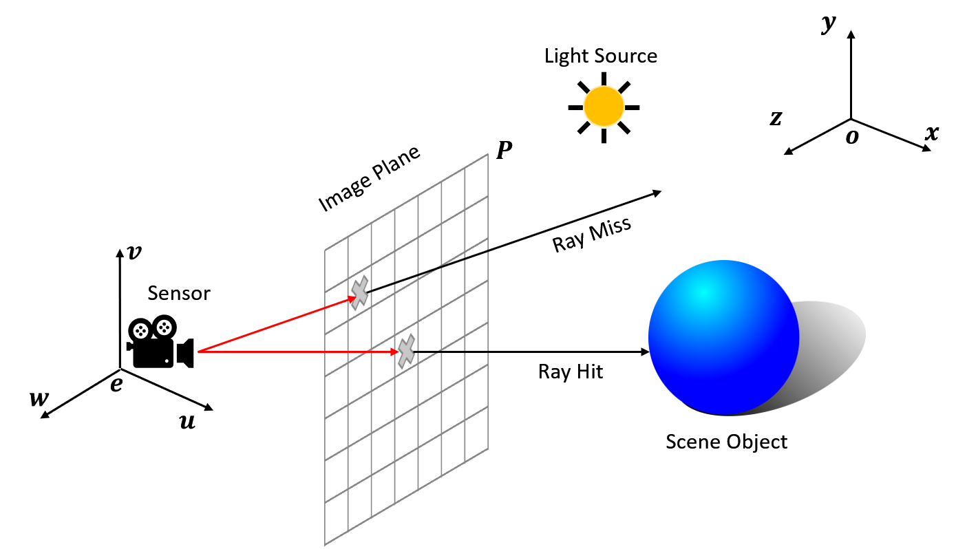
Figure 2: The ray tracing geometry: A ray cast from the sensor (camera), through the image plane, intersects the scene object in its course. The scene geometry and the light source (Sun) is set up in the $xyz$ world frame of reference, whereas the camera is aligned to a $uvw$ coordinate frame.

The intersection of the ray with any object in the scene is evaluated to assign a color to the pixels based on the intersection point. Note that each element of the rendering process, i.e., the ray and the 3D environment (comprising primitive geometries) are mathematical objects. Therefore, the intersection of the ray with these primitive geometries can be computed exactly. The intersection algorithms for a sphere and a triangle are discussed next.

2.1.3 Mathematical preliminaries for light matter interactions

In the ray tracer, the path of light is defined as a ray emanating from the origin of the sensor coordinate system, ${u}-{v}-{w}$ . The rendering engine computes intersections between light rays and the 3D objects in the environment. Given a sensor orientation, the first objective is to find the intersection of primary rays (the first rays cast into the environment) with any geometry in the scene. The type of objects in geometric models generally include spheres, triangles, rectangles, and in general polygons. The mathematical expressions for evaluating ray-triangle and ray-sphere intersections are delineated in the literature and adopted for this ray tracer engine [59]. Owing to their co-planar nature and efficient software realization, triangular meshes are adopted as primitive representations that build 3D geometries for models involving space based observations. The ray-primitive intersections are highlighted in Fig. 3 and their mathematical preliminaries are derived as follows.

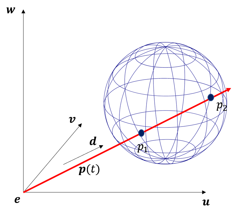
(a) The ray $\mathbf{p}(t)$ hits the sphere at points $p_{1}$ and $p_{2}$

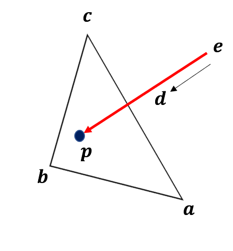
(b) The ray hits the plane containing the triangle at point $\mathbf{p}$

Figure 3: Intersection of a ray with a sphere and a triangle.

A ray $\mathbf{p}(t)$ may be mathematically described using the parametric equation of a line originating from the origin of the sensor coordinate system, $\mathbf{e}$ and advancing a distance of $\mathit{t}$ units in the direction $\mathbf{d}$

$$\mathbf{p}(t)=\mathbf{e}+\mathit{t}\mathbf{d}$$ (1)

The point of intersection of this ray, $\textbf{p}(t)$, with a sphere centered at c and having radius $R$ is obtained by solving the following equation:

$$(\mathbf{p}-\mathbf{c}).(\mathbf{p}-\mathbf{c})-R^{2}=0$$ (2)

Since the point at the intersection lies on both the ray in Eq. (1) and the sphere in Eq. (2), the values of $\mathit{t}$ on the ray are solved by substitution. This yields:

$$(\mathbf{e}+\mathit{t}\mathbf{d}-\mathbf{c}).(\mathbf{e}+\mathit{t}\mathbf{d}-\mathbf{c})-R^{2}=0$$ (3)

$$(\mathbf{d}.\mathbf{d})\mathit{t}^{2}+2\mathbf{d}.(\mathbf{e}-\mathbf{c})\mathit{t}+(\mathbf{e}-\mathbf{c}).(\mathbf{e}-\mathbf{c})-R^{2}=0$$ (4)

The roots of the quadratic equation in Eq. (4) determine the point of ray-sphere intersection. If the discriminant of the Eq. (4) is negative, then there are no intersections between the sphere and the ray. Conversely, a positive discriminant implies that there exist two solutions, each of which describe the points on the sphere where the ray enters and where the ray exits, respectively. If the discriminant is zero, then the ray grazes the surface of the sphere and touches it at exactly one point. Solving for the parameter $\mathit{t}$, we get the ray-sphere intersection point defined by

$$\mathit{t}=\frac{-\mathbf{d}.(\mathbf{e}-\mathbf{c})\pm\sqrt{(\mathbf{d}.(\mathbf{e}-\mathbf{c})-(\mathbf{d}.\mathbf{d})((\mathbf{e}-\mathbf{c}).(\mathbf{e}-\mathbf{c})-R^{2})}}{(\mathbf{d}.\mathbf{d})}$$ (5)

The unit surface normal vector $\mathbf{n}$ at the ray-sphere intersection point is given by $\mathbf{n}={(\mathbf{p}-\mathbf{c})}/{R}$. The angle between the light direction and the surface normal vector determines the spectral reflection at the intersection point, toward the sensor.

The intersection of a ray with a triangle may be computed using Möller-Trumbore algorithm, which uses barycentric coordinates and takes advantage of the parametric equation for a plane containing the triangle [60, 61]. The barycentric coordinates represent the intersection point $\mathbf{p}$ in terms of the non-orthogonal basis vectors formed by the vertices $\mathbf{a},\mathbf{b}$ and $\mathbf{c}$ of a triangle as follows:

$$\mathbf{p}(\beta,\gamma)=\mathbf{a}+\beta(\mathbf{b}-\mathbf{a})+\gamma(\mathbf{c}-\mathbf{a})$$ (6)

The intersection point, $\mathbf{p}$, is obtained by replacing the $\mathbf{p}$ with the parametric form of the ray in Eq. (1) as follows:

$$\mathbf{e}+t\mathbf{d}=\mathbf{a}+\beta(\mathbf{b}-\mathbf{a})+\gamma(\mathbf{c}-\mathbf{a})$$ (7)

In this representation using barycentric coordinate system [61], the point $\mathbf{p}$ is inside the triangle only if $\beta>0$, $\gamma>0$ and ${\beta}+{\gamma}<1$. Equation 7 is transformed into a linear system of equations and solved for $t$, $\beta$, and $\gamma$ using Cramer’s rule or matrix inversion.

$$\begin{bmatrix}\mathbf{a-b}&\mathbf{a-c}&\mathbf{d}\end{bmatrix}\begin{bmatrix}\beta\\ \gamma\\ t\end{bmatrix}=\begin{bmatrix}\mathbf{a-e}\end{bmatrix}$$ (8)

Utilizing the information about ray-primitive intersections, the rendering equation is formulated in the following section and methodologies to solve this equation are discussed.

3 Mathematical Formulation of the Rendering Equation

The interaction of light with the matter at the ray-surface intersection determines the shading i.e., the color, of the objects in the scene. The nature of shading depends on the optical properties and orientation of the objects and their surfaces, the amount of light (radiance) arriving at a point in the scene, and the viewpoint perspective of the sensor or eye observing the scene. The interaction between the light and the surface is described using a multidimensional function known as Bidirectional Reflectance Distribution Function (BRDF) [62], $\mathbf{f}_{r}$. The BRDF models the relationship between the incident radiance $L_{i}(\mathbf{x},\hat{\bm{\omega}}_{i})$ and the reflected radiance $L_{r}(\mathbf{x},\hat{\bm{\omega}}_{i},\hat{\bm{\omega}}_{o})$ at a point $\mathbf{x}$ on an illuminated surface [63]. With $\hat{\bm{\omega}}_{i}$ describing the direction of incoming light and $\hat{\bm{\omega}}_{o}$, the direction of outing light ray, the BRDF can be expressed as

$$\mathbf{f}_{r}(\mathbf{x},\hat{\bm{\omega}}_{i},\hat{\bm{\omega}}_{o})=\frac{dL_{r}(\mathbf{x},\hat{\bm{\omega}}_{i},\hat{\bm{\omega}}_{o})}{dL_{i}(\mathbf{x},\hat{\bm{\omega}}_{i})}$$ (9)

Using the BRDF function in Eq. (9), the reflected radiance at a point $\mathbf{x}$, with surface normal $\hat{\mathbf{n}}$, is computed by integrating all the incidence radiance arriving over a unit hemispherical area $\Omega$ as

$$L_{r}(\mathbf{x},\hat{\bm{\omega}}_{i},\hat{\bm{\omega}}_{o})=\int_{\Omega}\mathbf{f}_{r}(\mathbf{x},\hat{\bm{\omega}}_{i},\hat{\bm{\omega}}_{o})L_{i}(\mathbf{x},\hat{\bm{\omega}}_{i})(\hat{\bm{\omega}}_{i}.\hat{\mathbf{n}})d\hat{\bm{\omega}}_{i}$$ (10)

Eq. (10) is a local illumination model, and it represents only the local reflection of light as it hits the surface of the objects and does not capture absorption or refraction properties of the surface material. Hence, to truly capture the light-matter interaction, the total radiance leaving a surface, $L_{o}(\mathbf{x},\hat{\bm{\omega}}_{o})$, is modeled as the sum of the radiance emitted by the underlying surface $L_{e}$, and the reflected radiance, $L_{r}$

$$L_{o}(\mathbf{x},\hat{\bm{\omega}}_{o})=L_{e}(\mathbf{x},\hat{\bm{\omega}}_{o})+L_{r}(\mathbf{x},\hat{\bm{\omega}}_{i},\hat{\bm{\omega}}_{o})$$ (11)

Combining the Eqs. (10) and (11), we obtain the light-energy equilibrium approximated about a hemispherical differential area $\Omega$ at a surface point $\mathbf{x}$ as

$$L_{o}(\mathbf{x},\hat{\bm{\omega}}_{o})=L_{e}(\mathbf{x},\hat{\bm{\omega}}_{o})+\int_{\Omega}\mathbf{f}_{r}(\mathbf{x},\hat{\bm{\omega}}_{i},\hat{\bm{\omega}}_{o})L_{i}(\mathbf{x},\hat{\bm{\omega}}_{i})(\hat{\bm{\omega}}_{i}.\hat{\mathbf{n}})d\hat{\bm{\omega}}_{i}$$ (12)

Eq. (12) is referred to as the light transport equation or the rendering equation [31]. The solution to this equation determines the intensity of light at the surface point due to illumination from light or other surfaces in the 3D scene. The intensities at all the other surfaces are computed similarly, adding to the recursive nature of the light energy distribution. The recursive formulation of the rendering equation suggests that the light emitters are not the only sources of scene illumination, but surfaces in the scene scatter and reflect light back into the world—making it a global illumination problem. The physically based ray tracer model described in this paper solves the global illumination problem to capture the reflection, refraction, and absorption effects of light at each of the ray-surface intersection points.

The rendering equation (Eq. (12)) also calls upon the ray tracer to intelligibly follow or trace the path of a primary light ray that is cast from a light source. The tracing of paths for all such secondary rays is quintessential for rendering realistic scenes to produce a cumulative global illumination effect, and the ray tracer engine may also be addressed as a path tracer. The ray tracer engine developed in this work implements random walk based Monte Carlo techniques for solving the rendering equation. The Monte Carlo solution converts the integral problem into an expected value problem with a path probability density function (PDF) $p(\bar{x})$ for a sample path $\bar{x}$

$$I=\int f(\bar{x})dx=\int\frac{f(\bar{x})}{p(\bar{x})}.p(\bar{x})d\bar{x}=E\left[\frac{f(\bar{x})}{p(\bar{x})}\right]$$ (13)

The expected value is estimated from $N$ random sample paths $\bar{x}_{1},\bar{x}_{2},\bar{x}_{3},...,\bar{x}_{N}$ generated with the probability density function $p$

$$I=E\left[\frac{f(\bar{x})}{p(\bar{x})}\right]\approx\frac{1}{N}\sum_{i=1}^{N}\frac{f(\bar{x}_{i})}{p(\bar{x}_{i})}$$ (14)

Figure 4: This figure demonstrates the sampling of the ray tracer engine. The ray tracer shoots multiple rays through each pixel, in the directions specified by the BRDF. The intensities obtained in all the sample directions are averaged to evaluate the corresponding pixel intensity.

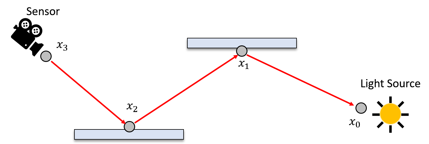
Figure 5: The ray tracer engine traces the path from the sensor to the light source to approximate the illumination at each surface point from the reflections at all other possible surfaces in the scene.

Equation (14) indicates that the contribution from all the samples is averaged to estimate the pixel intensities. This phenomenon is illustrated in Fig. 4. Cook [30] first presented this idea of stochastic or random sampling under the banner of distributed ray tracing. Rather than uniform sampling in all directions, Monte Carlo integration benefits from taking samples in the random directions proportional to the BRDF. Basing the probability distribution of the samples on the BRDF reduces the likelihood of choosing to sample directions near the horizon, where there is miniscule contribution to the illumination. This choice of sampling strategy, also called importance sampling reduces the variance because the estimator is close to the shape of the actual function. The importance sampling based unbiased estimation defines the PDF for a full path $\bar{x}$ as a product of conditional PDFs at the $n$ path vertices $x_{0},\,x_{1},\,...x_{n}$ as shown in Eq. (15) and illustrated in Fig. 5, where the full path is traced from the sensor to the light source (or sources) in order to approximate the illumination via Monte Carlo integration.

$$p(\bar{x})=p(x_{0},x_{1},x_{2},x_{3})=p(x_{3})p(x_{2}|x_{3})p(x_{1}|x_{2})p(x_{0})$$ (15)

This approximation of the pixel intensities improves with increasing number of samples per pixel, which is essential for rendering realistic images void of aliasing visual artifacts.

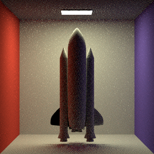
(a) Samples per pixel: 4

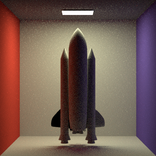
(b) Samples per pixel: 8

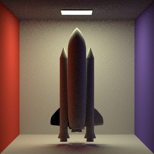
(c) Samples per pixel: 16

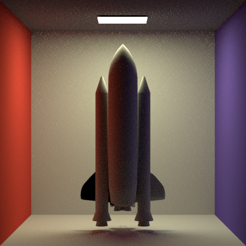
(d) Samples per pixel: 32

Figure 6: Effect of number of samples on image quality: The noise reduces with increasing the number of samples per pixel, which directly affects the approximation of the pixel color.

Figure 6 shows an example of the classical Cornell box [32] to distinguish the number of samples and the image quality.

3.1 Lighting model

While the evaluation of path tracing integral approximates pixel illumination, the optical properties that contribute to the illumination at a surface are governed by its material properties. BRDFs model the behavior of the material reflectance, at each surface points, for every incoming and outgoing directions as represented in Eq. (9). Fundamentally, the BRDF is a measure of the amount of light scattered by a surface from one direction to another. Integrating the BRDF in Eq. (10) over a specified incident and reflected solid angles determines the reflectance at a surface point. When a beam of light strikes a surface interface, it either gets scattered at the top or might penetrate into the material and undergo sub-surface or volumetric scattering. The majority of the scattering phenomenon occurs at the top layer, and it primarily depends on the refractive index of the illuminated medium. The topography of the interface determines the angular distribution of the scattered radiance - smooth surfaces reflect light into a specular direction, while rough surfaces reflect and diffuse light in many directions. Ideal diffusely reflecting or Lambertian objects appear equally bright from all viewing directions. Ultimately, the information on the nature of light-surface interaction is determined by the BRDF models for the objects. The BRDF models can be obtained from empirical measurements for various materials, which are fit into a mathematical function. Most BRDF models are generally a combination of specular and diffuse components. The Lambertian BRDF model assumes a constant BRDF value of, $\frac{\rho}{\pi}$ where $\rho$ (albedo) is the measure of diffuse reflection. While the Lambertian BRDF is effective for diffuse body reflections, it cannot accurately model specular surface reflections. The Phong lighting model [64] captures the effects of both the diffuse reflections from rough surfaces and the specular reflections from smooth surfaces. In this work, the Phong lighting model is considered to approximate the BRDF of space-object surfaces. The equation for the Phong model to compute the illumination at a surface point $x_{p}$ with normal $\hat{\mathbf{N}}$, per unit area perpendicular to the viewing direction $\hat{\mathbf{V}}$, is a combination of emissive ($I_{E}$), ambient ($I_{A}$), diffuse ($I_{D}$), and specular ($I_{S}$) illumination intensities.

$$I(x_{p},\hat{\mathbf{N}},\hat{\mathbf{V}})=k_{e}I_{E}+k_{a}I_{A}+k_{d}I_{D}(\hat{\mathbf{L}}.\hat{\mathbf{N}})+k_{s}I_{S}(\hat{\mathbf{R}}\cdot\hat{\mathbf{V}})^{n}$$ (16)

here, $k_{e}$, $k_{a}$, $k_{d}$, and $k_{s}$ are emissive, ambient, diffuse and specular constants that are exclusive to the type of surface materials. $\hat{\mathbf{L}}$ is the direction of light incidence and $\hat{\mathbf{R}}$ is the direction of reflection. The constant $n$ is used to regulate the size of specular highlights based on the material properties.

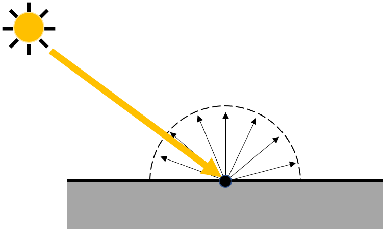
(a) Ideal diffuse, or Lambertian BRDF reflecting light equally in all directions

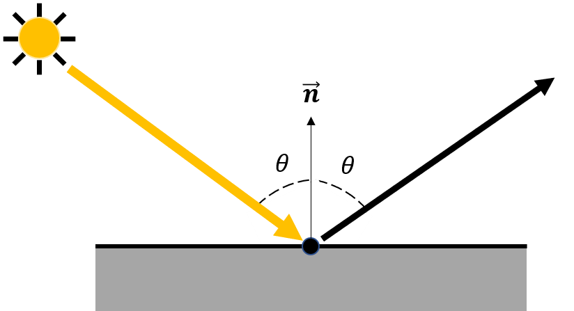
(b) Specular material reflecting light in the mirror direction

Figure 7: Lambertian and specular surfaces.

Recall that a ray cast into the scene might not stop upon hitting an object, and may undergo reflection or refraction at the ray-surface intersection and further cast into the scene. The ray tracer based rendering program under discussion is a global illumination method that accounts for shadows and effects such as reflection, refraction, scattering, indirect reflection, and indirect diffuse. The effect of shadows is determined by computing if a ray from a surface point hits an object on its path to the light sources. If it does, the point is categorized to be in a shadow as shown in Fig. 8.

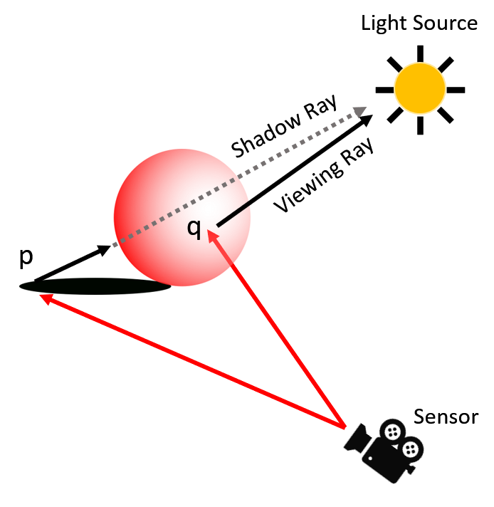
Figure 8: This figure demonstrates the method of computing shadows by tracing the light from the sensor to the source. In this demonstration, the surface point $\mathbf{p}$ is in shadow while the point $\mathbf{q}$ is not in shadow.

The specular reflection (reflection of light in mirror direction) is evaluated using the specular term of the Phong lighting model described in Eq. (16). The reflected ray $\hat{\mathbf{R}}$ is computed according to the law of reflection as

$$\hat{\mathbf{R}}=\hat{\mathbf{V}}+2\left(\hat{\mathbf{V}}.\hat{\mathbf{N}}\right)\hat{\mathbf{N}}$$ (17)

The rendering algorithm evaluates the reflection for a maximum recursion depth of 40 to balance the speed of the rendering process and the accuracy of the reflection effect. Snell’s law of refraction is implemented to model the effects of bending of light at a specular interface, between two media with refractive indices $n$ and $n_{t}$, $\theta$ angle of incidence and $\phi$ angle of refraction, as

$$n\sin\theta=n_{t}\sin\phi$$ (18)

The transmitted ray $\hat{\mathbf{T}}$ can be described from the basis formed by the orthonormal vectors $\hat{\mathbf{N}}$ and $\hat{\mathbf{B}}$ as

$$\hat{\mathbf{T}}=\sin\phi\hat{\mathbf{B}}-\cos\phi\hat{\mathbf{N}}$$ (19)

$\hat{\mathbf{B}}$ can also be obtained from the $\hat{V}$ described in the same basis,

$$\hat{\mathbf{V}} =\sin\theta\hat{\mathbf{B}}-\cos\theta\hat{\mathbf{N}}$$ (20)

$$\hat{\mathbf{B}} =\frac{\hat{\mathbf{V}}+\hat{\mathbf{N}}\cos\theta}{\sin\theta}$$ (21)

The reflection of light from a non-conducting or dielectric interface between two media varies according to the Fresnel equations. Schlick’s approximation [65] method approximates the Fresnel equations for an efficient computation of reflectivity ($R$) as

$$R(\theta)=R_{0}+(1-R_{0})(1-\cos\theta)^{5}$$ (22)

where $R_{0}$ is the reflectance at normal incidence:

$$R_{0}=\left(\frac{n_{t}-1}{n_{t}+1}\right)^{2}$$ (23)

3.2 Acceleration structure of the ray tracer engine

The recursive evaluation of rendering equation (Eq. (12)) evaluates each ray against every intersection in the scene. This brute force search for ray-surface intersection is inefficient and computationally very expensive. Kay and Kajiya [66] presented a technique called bounding volume hierarchy (BVH) as a method to accelerate ray tracing. The fundamental idea of BVH is to place multiple bounding boxes around all the objects in the scene geometry. The bounding boxes are hierarchically-arranged as a tree-based structure, with a large bounding box as a root and smaller bounding boxes within it as subtrees. Using this technique, it is tested if a ray intersects with the volume defined by the bounding boxes instead of the entire scene space to speed up the computation of ray-surface intersection. The engine creates a BVH structure from the source geometry prior to rendering a scene.

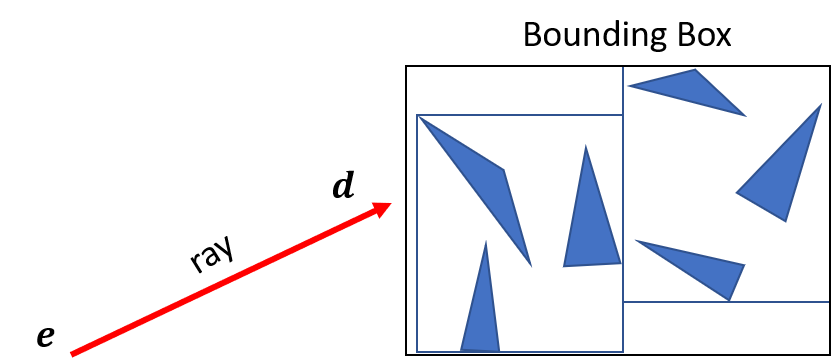
Figure 9: This figure illustrates the nested representation of the bounding boxes. Boxes created around the geometric primitives of the model and are nested inside another bounding box. The ray is only tested for intersection with objects if it hits the bounding box.

3.3 Capabilities

The capabilities of the NaRPA platform are outlined in the rest of this section. These capabilities include texture mapping, global illumination effect, depth of field effect, point cloud, depth map, and contour map generation [67]. They are described as follows:

• Texture mapping: Texture mapping [68] technique allows one to project a complex pattern (texture) on a simple polygon. The pattern may be repeated many times on to tile a plane, or it can be a multidimensional image projected onto a multidimensional space. 2D texture mapping associates the 2D coordinates $(u,v)\in[0,1]^{2}$ that correspond to a location in the texture image with points on a 3D surface. This is accomplished in two phases. First the $(u,v)$ space is mapped to object space $(x_{o},y_{o},z_{o})$ by parameterizing the surface followed by transforming the object onto a screen, by the rendering engine. As an example, spherical coordinate parameterization to map a texture image onto a sphere is shown in Fig. 10. With the NaRPA’s ability to generate texture mapped primitives, clusters of objects can be conveniently represented to maintain high frame rates and high level of details to aid in visual navigation [69].

  

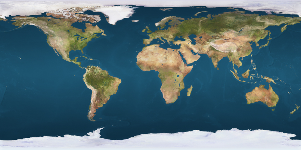
  (a) Earth surface texture map as a 2D image

  

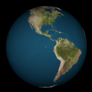
  (b) Texture projected onto a sphere

  Figure 10: This figure illustrates the 3D texture mapping capabilities of the ray tracer. 2D image coordinates that correspond to the Earth are projected onto a sphere to model the Earth in free space.

  Let $-\pi\leq\theta\leq\pi$ be the latitude angle around the sphere in the horizontal plane and $0\leq\phi\leq\pi$ be the longitude angle measured from $0$ at the South Pole to $\pi$ at the North Pole. The parametric equation of a sphere with radius $R$ and center $(x_{c},y_{c},z_{c})$ is

  $$x_{o} =x_{c}+R\cos\phi\sin\theta$$ (24)

  $$y_{o} =y_{c}+R\sin\phi\sin\theta$$ (25)

  $$z_{o} =z_{c}+R\cos\theta$$ (26)

  and

  $$\theta =\cos^{-1}\left(\frac{z_{o}-z_{c}}{R}\right)$$ (27)

  $$\phi =\tan^{-1}\left(\frac{y_{o}-y_{c}}{x_{o}-x_{c}}\right)$$ (28)

  Now, defining

  $$u =\frac{\phi}{2\pi}$$ (29)

  $$v =\frac{\pi-\theta}{\pi}$$ (30)

  allows us to index the $(u,v)$ of the texture map for all the points on the surface of the sphere. This mapping is shown in the Fig. 10.

• Global illumination: The ray tracing engine presented in this paper is a global illumination algorithm. Simulating the effects of both direct and indirect illuminations to render a realistic image from the scene description defines the term global illumination. Direct illumination is a result of intersection between light rays from the source and the object surface. Indirect illumination stems from the multiple complex reflections that the rays undergo before exiting the scene geometry. Figure 11 illustrates the effects of global illumination from a render of fictional scene geometry by the ray tracer engine. In Figure 11, while the top hemisphere of the moon is illuminated by direct light, the bottom surface observes illumination due to reflections from the Martian surface, depicting the effects of global illumination. This effect is a key aspect to generate reliable simulations for developing computer vision algorithms aimed at vision-based navigation [70].

  

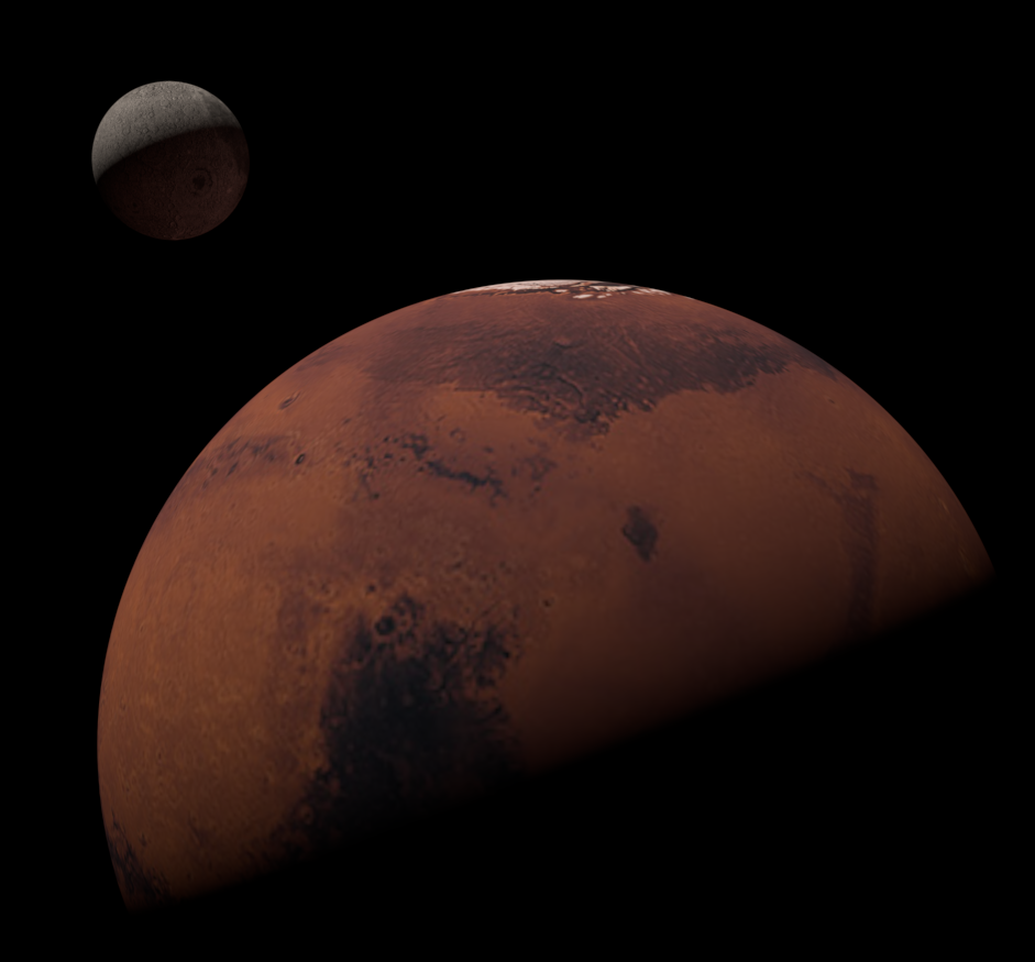
  Figure 11: This figure demonstrates the global illumination effect through a fictitious free space environment with the Mars and the Moon as objects. Notice the bottom hemisphere of the moon being illuminated by multiple reflections from the Martian surface, while direct sunlight illuminates the top hemisphere.

• Depth of field effect: Imaging sensors have an aperture through which light enters the sensor to register an image on the sensor film. A smaller aperture increases the depth of the scene which is in focus, and the objects in the scene appear sharp when rendered. Using a larger aperture, in combination with a lens, allows more light into the sensor but is less controlled. The 3D objects at the focal length are projected into a single point on the sensor, while the other points map into a blur circle. The latter effect, resulting in a blurred portion of the image from objects at certain distance, is known as depth of field or the defocus blur effect. Defocus effects are commonly encountered because of large relative distances among planetary objects. Therefore, it is essential to simulate navigation scenarios with attribution to the defocus and motion blur effects [71].

  

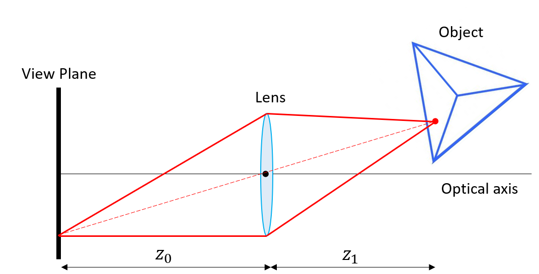
  Figure 12: Thin lens system with the light rays from the object converge at a point on the view plane, reckoning the object point to be in focus.

  The ray tracing engine adopts a thin lens model for the virtual camera to generate depth of field effects [72]. In the thin lens model, the rays of light emitted from a surface point travel through the lens and converge at a point behind the lens, as shown in Fig. 12. The focal length (distance between the point of projection and the image plane), $f$, defines this characteristic of the thin lens and is modeled using the lens equation

  $$\frac{1}{f}=\frac{1}{||z_{0}||}+\frac{1}{||z_{1}||}$$ (31)

  The thin lens approximation for the virtual camera of the ray tracer engine simulates the depth of field effect by controlling the focus distance (distance from the point of projection and the object plane in focus) and/or the aperture radius. From Eq. (31), the distance between the view plane and the lens (projection point) for a given focal length $f$ and a focus distance $d_{f}$ is

  $$z_{0}=\frac{fd_{f}}{d_{f}-f}$$ (32)

  Eq. (32) represents the distance at which the projection of an object or a point that is in focus at a distance $d_{f}$ in front of the lens, will converge behind the lens. If the film is located at $z_{0}$, the projection of the object converges to a point and otherwise to a circle of confusion (COC) to appear as a blurred spot. Figure 13 shows the depth of field effect with a fixed focus distance and increasing aperture radius to observe the defocus blur effect on the ISS with the moon in the background.

  

  (a) Aperture radius: 0 (pinhole model)

  

  (b) Aperture radius: 0.04

  

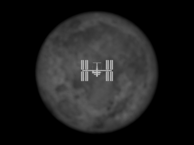
  (c) Aperture radius: 0.06

  

  (d) Aperture radius: 0.15

  Figure 13: This figure illustrates the defocus blur effect with the International Space Station (ISS) in focus and an incremental blurring effect on the moon due to widening of the camera aperture (scene units).

• 3D Point Cloud, Depth, and Contour Maps: Point cloud data is generally acquired by 3D imaging sensors such as LiDAR (Light detection and ranging). NaRPA stores the 3D location of the first point of intersection between each ray and the objects in the scene. It uses the light propagation time to compute range to different objects in the scene. This simulates the characteristic feature of LiDAR type scanners and depth cameras and thereby takes advantage of the existing ray tracer algorithm to generate point clouds and depth maps. The engine also accommodates simulation of velocimetry LiDAR sensing from continuous sweeps of LiDAR scans. Figure 14 shows the point cloud data extracted from the digital elevation model (DEM) of Curiosity landing site within the Gale crater of Mars. Depth and contour maps are generated from the elevation data of the DEMs. By the inclusion of physically-based simulator of LiDAR sensors, NaRPA has the capabilities to generate true physical data and enable testing of registration algorithms for spacecraft relative navigation [73, 74].

  

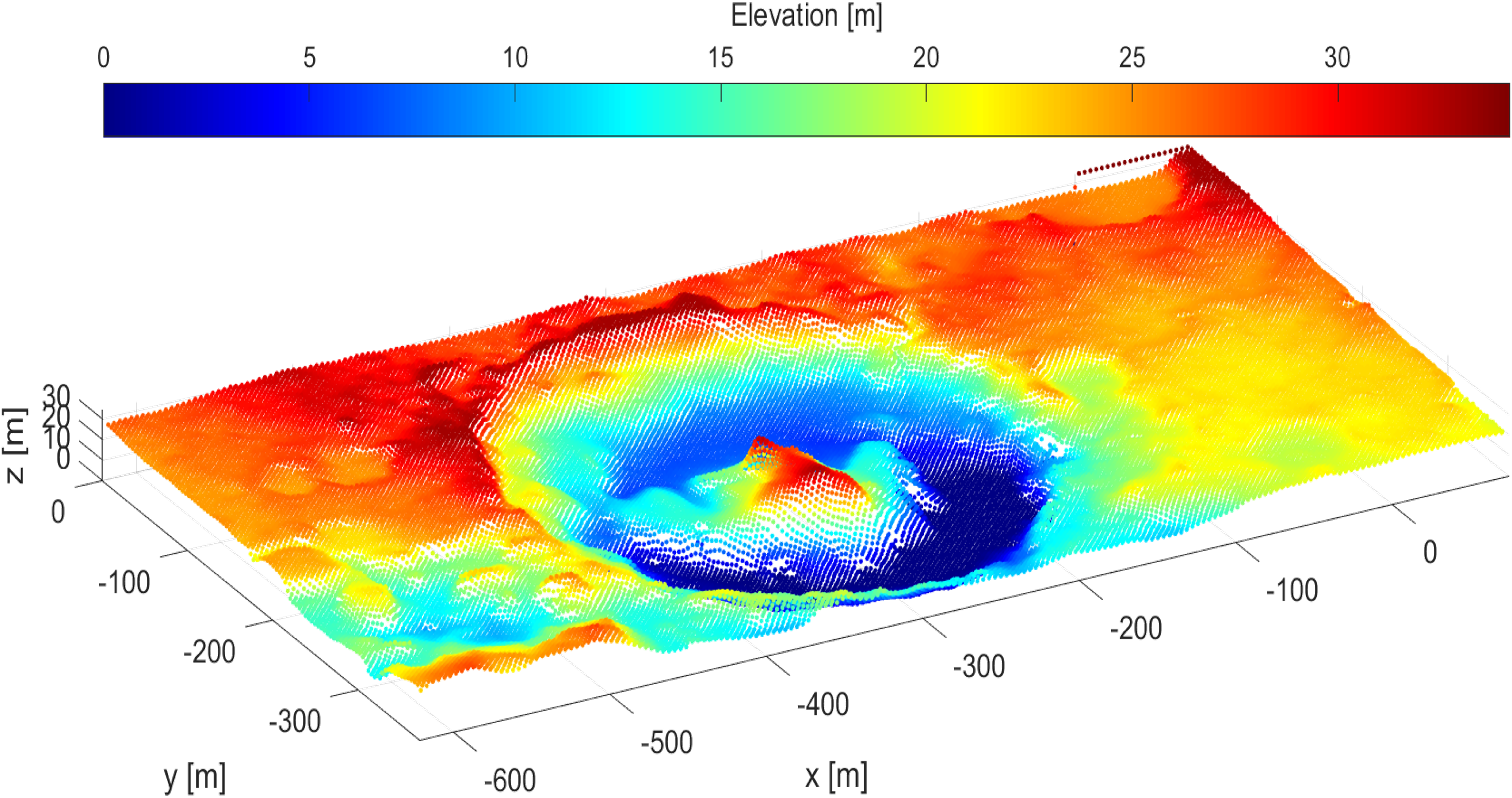
  (a) 3D point cloud data of Curiosity landing site

  

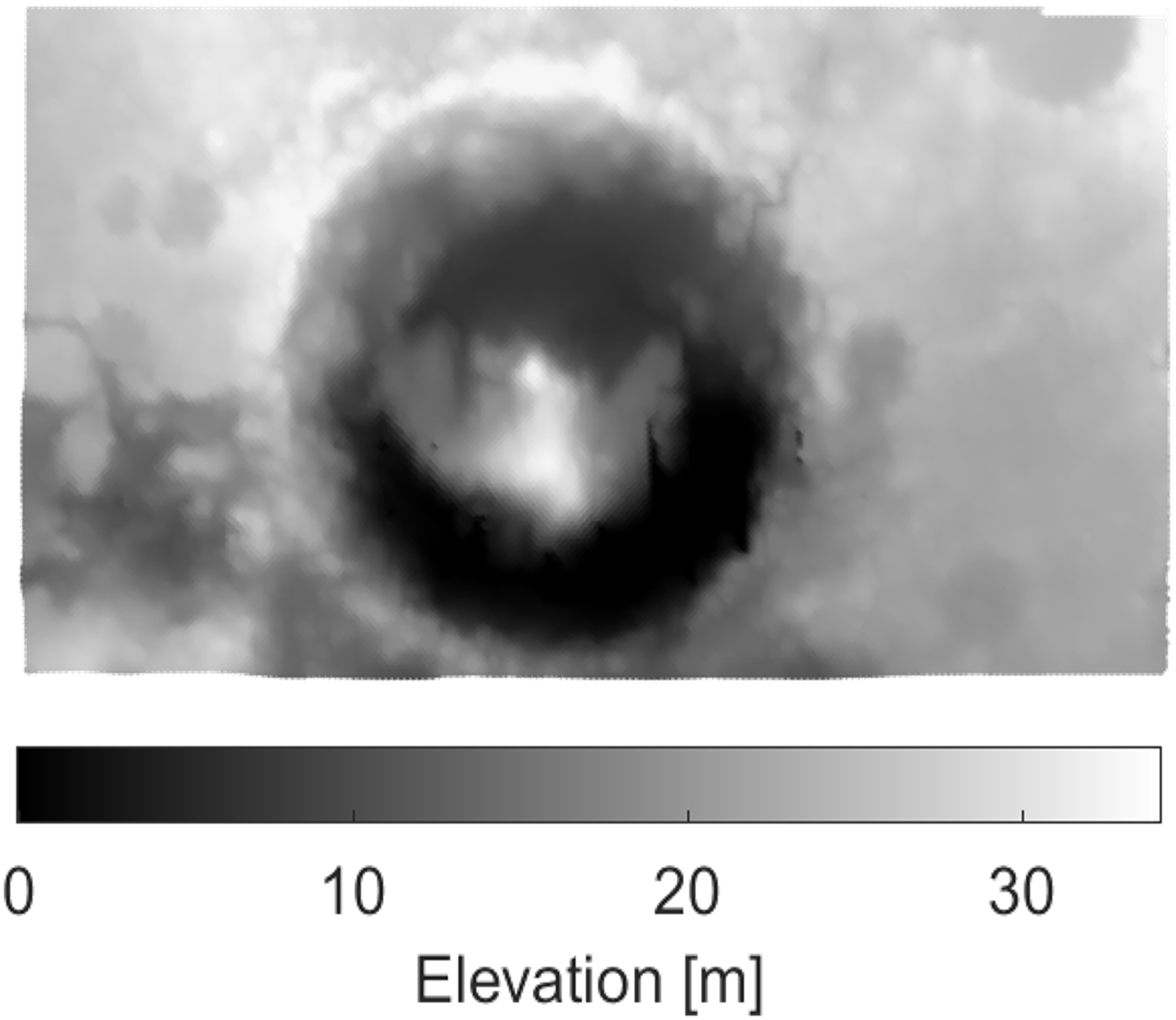
  (b) Depth map of the Curiosity landing site

  

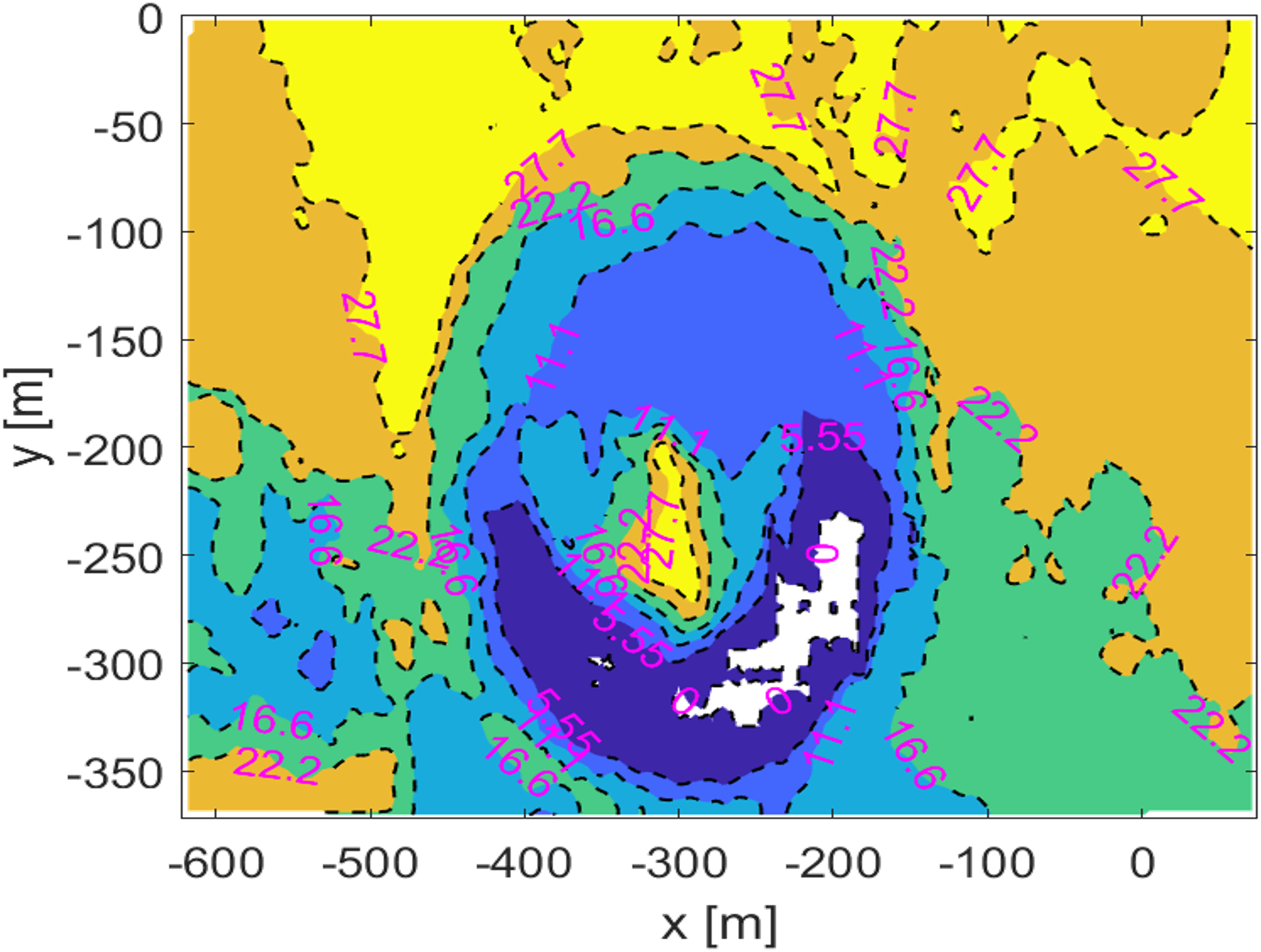
  (c) Contour map of the Curiosity landing site

  Figure 14: This figure demonstrates the simulation of a LiDAR sensor configured on a spacecraft approaching vertically down. The data corresponding to point cloud, depth and contour maps is obtained from the ray tracer engine configured with the virtual LiDAR scanner.

4 Atmospheric Modeling and Rendering Ground-based Observation of Space Objects

The scattering of light due to particles present in the atmosphere influence the appearance of an object. The particles or gas molecules redirect the light rays from their original path and effect the colors of the object observed in natural light. The methods to simulate the scattering effects of the atmosphere are described by Nishita et al. [34]. Preetham et al. [59] proposed an analytical model which provides an accurate simulation of the sky colors, and it is more restrictive in that the model only works for an observer located on the ground. The methods of atmospheric scattering simulations in this paper borrows from the work of Nishita and Preetham [34, 59] and is outlined in the following section. Additionally, the contributions of Tessendorf [75, 76, 77, 78, 79, 80] have been adopted to embed multiple scattering effects for atmospheric rendering.

4.1 Atmospheric model

Atmosphere is a thin blanket of gases enveloping a planet. The atmosphere in held in its place by the planet’s gravity, and it is defined in multiple layers basis their temperature distribution and composition. Earth’s atmosphere thickness is about 100 km and is made of oxygen, nitrogen, argon, carbon dioxide, water vapor, and other floating particles classified as aerosols which include dust, pollen, smoke, and more. In this paper, a thickness of 60 km is used by considering scattering of light rays in only the two lower layers of the Earth’s atmosphere - troposphere and the stratosphere. Photons, travelling through the Earth’s atmosphere in a certain direction, are deflected in various directions when they collide with the particles in the atmosphere. The dispersion and diffusion of light as a result of atmospheric scattering depends on the size and density of particles in the atmosphere. The density or tightness of these particles decreases with altitude. Thus, the number of molecules per cubic volume is relatively low in the upper layers of the atmosphere.

The scattering is computed by sampling the atmospheric density along the light ray at regular intervals. As a first step, the scattering of light is approximated by a forward refraction. A fundamental approach [34] is to determine the scattering from the assumption of exponential decrease in the atmosphere density with altitude modelled with an equation of the form:

$$\rho(h)=\rho(h_{0})\exp\Big{(}-\frac{h}{H}\Big{)}$$ (33)

where $\rho(h_{0})$ is the density of air at sea level, $h$ is the current altitude above the sea level and $H$ is the thickness of the atmosphere if its density were uniform. Using this information on density and a similar model of the pressure distribution of air molecules in the atmosphere, we utilize a model that states the refractive index of the atmosphere at a particular height above the Earth’s surface. Exponential refractive index model with altitude dependence of refractive index is given by

$$(n(h)-1)\times 10^{6}=\frac{79\left(P+\frac{4800e}{T}\right)}{T}\hskip 28.45274pt\begin{cases}\text{For Troposphere (<12 km)}&T=59-0.00356h\\ &P=2116\left(\frac{T+459.7}{518.6}\right)^{5.256}\\ \text{For upper atmosphere (>12 km)}&T=-70\\ &P=473.1\exp(1.73-0.000048h)\end{cases}$$ (34)

Here, $n(h)$ is the average refractivity at height $h$, $T$ is the temperature, $P$ is the pressure and $e$ is the density of water vapour and other gasses given by Eq. (33). The refractive index is modelled as a series of spherically concentric shells for computational advantage. The atmosphere modeled as a series of spherical shells considers higher number of samples at lower altitudes where the density is high and lower number of samples at higher altitude where the air is less dense. This technique of ‘importance sampling’ improves upon the convergence speed relative to a ‘constant step’ integration method. Since the density increases exponentially with altitude, numerical integration involved in ray tracing is performed over small intervals at low altitude and larger intervals at high altitudes. The setup is illustrated in the following figure 15:

Figure 15: Refractive Index model

The scattering of light depends strongly upon the size of the particles in the atmosphere. If the scattering is due to particles that are smaller than the wavelength of the light, then it is called Rayleigh scattering. In Rayleigh scattering, incident light is scattered more heavily at the shorter wavelengths. If the incident light is scattered equally in all directions, it is called Mie scattering. Larger particles in the air called aerosols (dust, pollen) cause the Mie scattering. To capture the effect of Rayleigh scattering, the spherical shells are modelled with varying refractive indices for each sample of the ray generated and the depth for each ray to be slightly different (using a pseudo-random number). Since, the aerosol distribution is only limited to the lower atmosphere, Mie scattering effects are captured using the above proposed method for spherical shells lying below a particular altitude.

Note here that in the description of our model, the Sun is the source of illumination of the sky. The Sun is assumed to be at a considerable distance from the Earth, and the light rays reaching the atmosphere are parallel to one another. This is also observed to be similar to the inbuilt sky emitter in Mitsuba renderer [50].

4.1.1 Atmospheric modeling and ground-based space object simulation results

Simulations for ground-based space object observations in the presence of atmospheric scattering effects are delineated through the following rendering exercise. The renderer is enabled to simulate observations at different times of a day, borrowed from the sky-dome radiance model by Hošek and Wilkie [81]. The daylight renderings of the ISS at different times of the day are shown in Fig. 16. This exercise emulates the fully-focused telescopic observation of the ISS placed in the low-earth orbit. The model evaluates the turbidity of the atmosphere and the position of the emitter. Turbidity characterizes the scattering of light by aerosol content in the atmosphere. Increasing the levels of turbidity increases the scattering of light rays and decreases the intensity of radiation. The renderings of the ground-based ISS observations at different levels of turbidity are shown in Fig. 18. The effects of lower visibility can be offset by increasing the exposure of the virtual camera. The simulation results with variation in the exposure levels are shown in Fig. 17. In this exercise, the exposure levels are specified in f-stops, which in turn specify aperture radius. Higher exposure levels upscale the radiance values applied to the image to result in a brighter output.

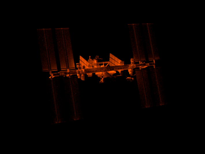
(a) 7:20 AM

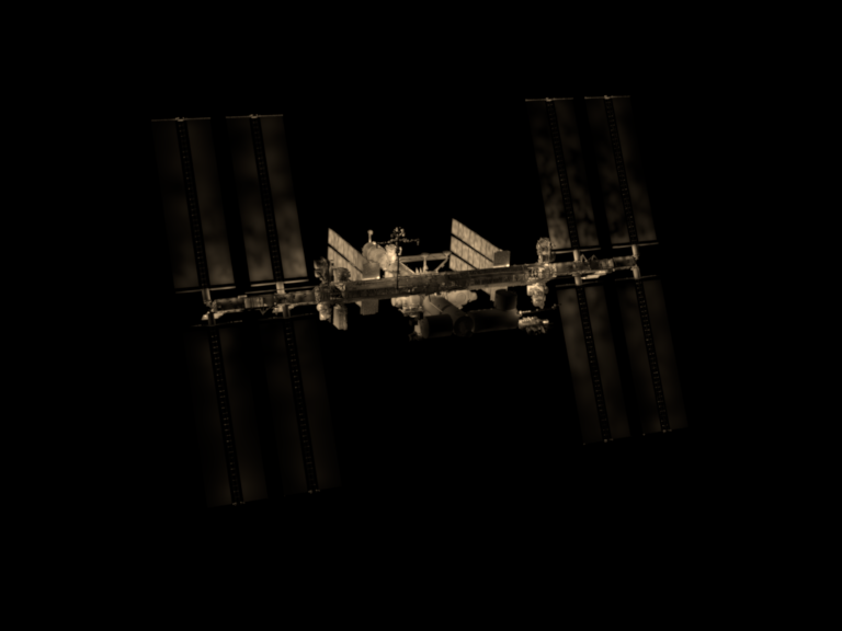
(b) 8:20 AM

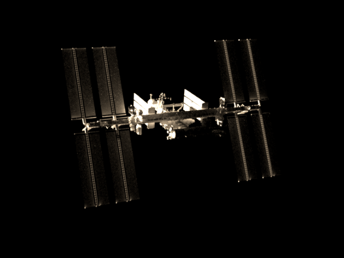
(c) 6:20 PM

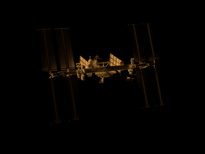
(d) 7:20 PM

Figure 16: Ground-based observation of the ISS, illustrating renderings at different times of a day.

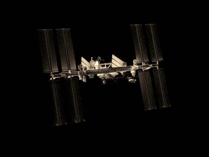
(a) Turbidity level: 1

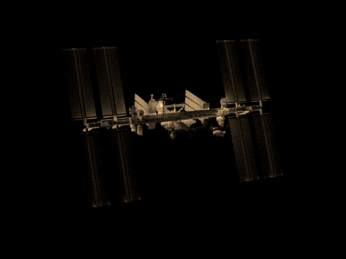
(b) Turbidity level: 3

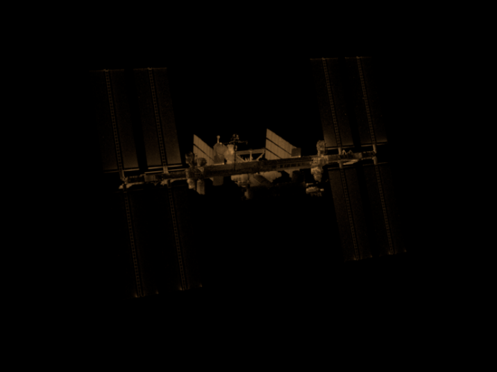
(c) Turbidity level: 6

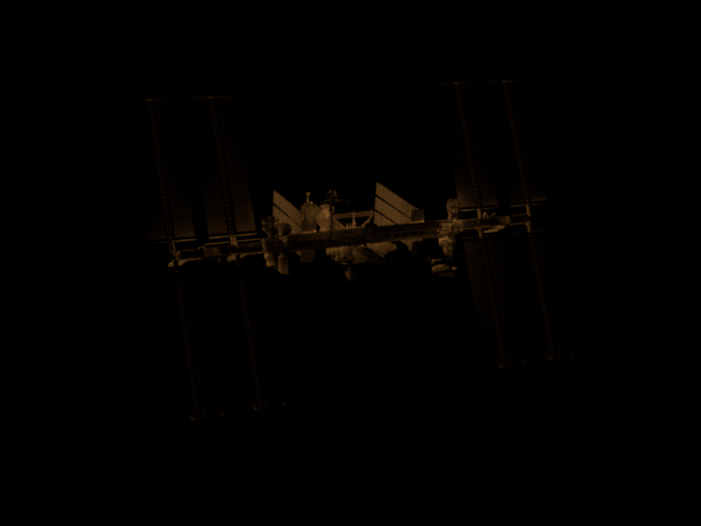
(d) Turbidity level: 8

Figure 17: Ground-based observation of the ISS, illustrating renderings at different values of turbidity.

(a) Exposure: $2^{0}$

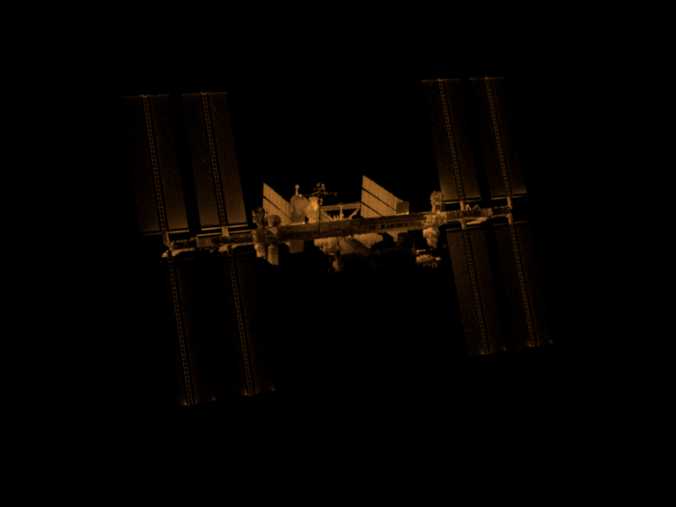
(b) Exposure: $2^{1}$

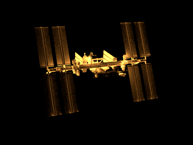
(c) Exposure: $2^{2}$

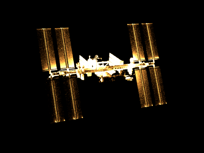
(d) Exposure: $2^{3}$

Figure 18: Ground-based observation of the ISS, illustrating renderings at different values of exposure. The exposure factors are specified in f-stops, which is a measure of the camera’s aperture radius.

5 Depth Estimation using Stereo Vision

Computing depth from 2D images remains one of the widely studied topic in vision based navigation [82, 83, 84]. Classical approaches for depth estimation rely on stereo matching via pixel correspondence across images captured from a stereo camera setup. Depths are estimated by triangulation, wherein each corresponding pair of image coordinates are used to estimate the respective 3D coordinates in the scene. Modern approaches utilize deep learning frameworks for depth retrieval and 3D reconstruction tasks [85]. In either approaches, availability of high fidelity ground truth data is monumental in testing and validating the depth estimation algorithms.

In this paper, NaRPA is applied as an engine for generating custom resolution stereo imagery. The rendering engine is capable of generating stereo images for 3D coordinate estimation using calibrated and uncalibrated stereo vision. We demonstrate depth computation in a calibrated stereo application using the classical triangulation approach. As a motivating example, consider the motion of a spacecraft in relative navigation with respect to a planetary terrain, as shown in Fig. 19. Two key-frames are observed in the stereoscopic setup, emulating a motion from stereo application. The coordinate transformation between the two capturing events are assumed to be available from onboard sensors in a terrain-fixed reference frame.

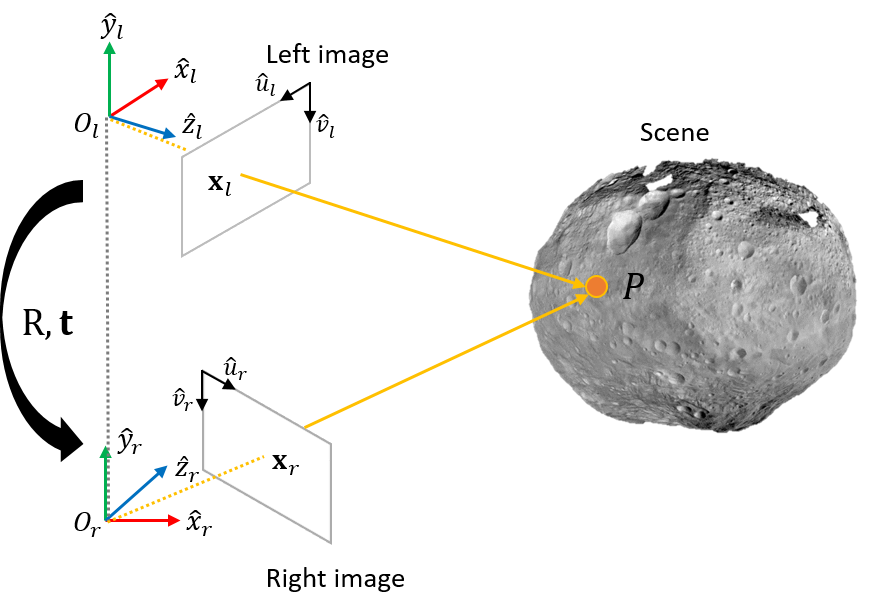
Figure 19: Triangulation to show the relationship between the scene point $P$ and its projections in the left and right camera frames, centered at $O_{l}$ and, $O_{r}$ respectively.

5.1 Stereoscopic System Model

Epipolar geometry relates the multi-view images of the observed scene to the 3D object in the scene [86]. It represents a geometric relation between the spatial coordinates in the scene and their image projections in a stereoscopic setup. Consider an object point $P\in\mathbb{R}^{3}$ and its two images in left and right camera frames, given by their coordinates $\mathbf{x}_{l}=[x_{l},y_{l},z_{l}]$ and $\mathbf{x}_{r}=[x_{r},y_{r},z_{r}]$. The $\mathbf{x}_{l}$, $\mathbf{x}_{r}$, and $P$ are related by the triangular geometry shown in Fig. 19. Perspective projection geometry governs the mapping from 3D coordinates onto 2D image plane coordinates, as shown below.

For calibrated pinhole camera sensors with known intrinsics, the projections of $P$ in the left and right image planes are given by

$$\frac{U_{i}}{f_{x}^{(i)}}=\frac{u_{i}-o_{x}^{(i)}}{f_{x}^{(i)}}=\frac{x_{i}}{z_{i}}$$ (35)

$$\frac{V_{i}}{f_{y}^{(i)}}=\frac{v_{i}-o_{y}^{(i)}}{f_{y}^{(i)}}=\frac{y_{i}}{z_{i}}$$ (36)

where $i$ is a placeholder to indicate left, and right camera coordinate frames ($l$ and $r$). $u_{i}$ and $v_{i}$ are the image projections of $P$ in the left and right image planes. $U_{i}$ and $V_{i}$ are the shorthand notation for image-centered pixel coordinates. Focal lengths ($f_{x}^{(i)},f_{y}^{(i)}$) and principal point offsets ($o_{x}^{(i)},o_{y}^{(i)}$) denote the camera intrinsic parameters of the left and right cameras.

The homogenous coordinates $\mathbf{x}_{l}$ and $\mathbf{x}_{r}$ are related by a known transformation between the left and the right camera frames as

$$\begin{bmatrix}x_{r}\\ y_{r}\\ z_{r}\\ 1\end{bmatrix}=\begin{bmatrix}R_{11}&R_{12}&R_{13}&t_{x}\\ R_{21}&R_{22}&R_{23}&t_{y}\\ R_{31}&R_{32}&R_{33}&t_{z}\\ 0&0&0&1\end{bmatrix}\begin{bmatrix}x_{l}\\ y_{l}\\ z_{l}\\ 1\end{bmatrix}$$ (37)

The division of $x_{r}$ with $z_{r}$ in Eq. (37) yields the right-hand side expression of the perspective projection equation (35)

$$\frac{x_{r}}{z_{r}}=\frac{R_{11}x_{l}+R_{12}y_{l}+R_{13}z_{l}+t_{x}}{R_{31}x_{l}+R_{32}y_{l}+R_{33}z_{l}+t_{z}}$$ (38)

$$\frac{x_{r}}{z_{r}}=\frac{R_{11}\frac{x_{l}}{z_{l}}+R_{12}\frac{y_{l}}{z_{l}}+R_{13}+\frac{t_{x}}{z_{l}}}{R_{31}\frac{x_{l}}{z_{l}}+R_{32}\frac{y_{l}}{z_{l}}+R_{33}+\frac{t_{z}}{z_{l}}}$$ (39)

Now, by substituting the perspective projection equations (35 & 36), we obtain

$$\frac{U_{r}}{f_{x}^{(r)}}=\frac{R_{11}\frac{U_{l}}{f_{x}^{(l)}}+R_{12}\frac{V_{l}}{f_{y}^{(l)}}+R_{13}+\frac{t_{x}}{z_{l}}}{R_{31}\frac{U_{l}}{f_{x}^{(l)}}+R_{32}\frac{V_{l}}{f_{y}^{(l)}}+R_{33}+\frac{t_{z}}{z_{l}}}$$ (40)

Upon simplification, $z_{l}$, the $z$ coordinate of $P$ in the left camera frame, is expressed as

$$z_{l}=\frac{t_{z}U_{r}-f_{x}^{(r)}t_{x}}{\left(R_{11}f_{x}^{(r)}-R_{31}U_{r}\right)\frac{U_{l}}{f_{x}^{(l)}}+\left(R_{12}f_{x}^{(r)}-R_{32}U_{r}\right)\frac{V_{l}}{f_{y}^{(l)}}+\left(R_{13}f_{x}^{(r)}-R_{33}U_{r}\right)}$$ (41)

Using the projection equations again, the $x$ and $y$ coordinates of $P$ in the left camera frame are recovered as

$$x_{l}=z_{l}\frac{U_{l}}{f_{x}^{(l)}}$$ (42)

$$y_{l}=z_{l}\frac{V_{l}}{f_{y}^{(l)}}$$ (43)

Using the geometric relationship between the left and the right camera frames along with their corresponding image plane projections, the 3D scene coordinates $\mathbf{x}_{l}$ , in the left camera frame (or $\mathbf{x}_{r}$, if parameterized, in the right camera frame) are determined.

5.2 Results

5.2.1 Scene Configuration

Two imaging events in a planetary descent simulation are rendered in this exercise for 3D coordinate estimation using triangulation. Two monocular images of a terrain are captured at two deterministic poses in the virtual scene geometry, with the terrain under sufficient illumination. The geometric parameters for imaging are captured in Table 1. Optical specifications include pinhole camera resolution of $500\times 500$ pixels, diagonal field-of-view of $30^{\circ}$. Computation of 3D feature coordinates is performed according to the following principles:

• Image correspondence via stereo matching is established via sparse corner features extracted using Eigenvalue-based geometrical feature detection [87]. The matching stereo pairs $\mathbf{p}_{l}$ and $\mathbf{p}_{r}$ are acquired from the descriptors of the corner features detected in the key frames.

• 3D terrain coordinates are realized by computing the expressions in Eqs. (41, 42, 43).

• For verification, ground truth is established from the NaRPA generated point cloud of the object (see Section 3.3) as well as the known transformation from individual camera frames to the terrain-fixed reference frame.

Target (m)	Origin (m)	Up (rad)
$[0\quad 0\quad 0]^{T}$	$[0\quad 0\quad 800]^{T}$	$[1\quad 0\quad 0]^{T}$
$[0\quad-30\quad 0]^{T}$	$[0\quad-30\quad 750]^{T}$	$[1\quad 0\quad 0]^{T}$

Table 1: Geometric parameters for camera positioning and orientation in the scene: ‘Target’ indicates the camera pointing location, ‘Origin’ indicates the camera position, and ‘Up’ represents the camera alignment.

5.2.2 Results

3D coordinates are estimated in the left camera frame ($\hat{\mathbf{x}}_{l}$) and the percentage of relative errors along each of the coordinates is calculated as

$$\%\text{Error}=\frac{|\hat{\mathbf{x}}_{l,i}-\mathbf{x}_{l,i}|}{|\mathbf{x}_{l,i}|}\times 100\hskip 142.26378pti=1,2,3$$ (44)

The estimated 3D coordinates are reprojected into the left camera frame using the known camera intrinsics. The estimated and the true pixel coordinates are highlighted in Fig. 20a. Figure 20b shows the distribution of absolute errors as well as the percentage of relative errors in 3D coordinate estimation. Maximum absolute errors are observed to be along the $z$ coordinates, which is expected due to the placement of the camera relatively farther along $z$. Outliers in the percentage of relative errors are more along $y$ because the $y$-coordinates of these feature points are very close to $0$ (leaving a significant quotient in the division of two close floating point values).

(a) True and estimated pixel projections (bottom 20 matches)

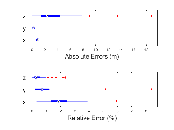
(b) Errors in the $x,y,z$ estimates evaluated for 100 feature points. Outliers are indicated by +.

Figure 20: This figure depicts the 3D coordinate estimation results. On the left, the estimated coordinates are reprojected into the camera frame for visual comparison. On the right, absolute, and relative error distributions between the estimated and the true coordinates are portrayed.

In this capability demonstration, the 3D coordinates are not estimated to sub-pixel accuracy. But, using dense point correspondences from NaRPA renderings, effective outlier rejection schemes, and efficient pixel interpolation schemes, applications such as structure from motion and 3D scene reconstruction are realizable.

6 Differentiable Rendering for Relative Pose Estimation

Determination of relative pose between the spacecraft and a target satellite is one of the critical tasks in autonomous proximity operations. Monocular vision based guidance and navigation is a much researched topic in this regard [88, 89]. NaRPA provides a virtual experimental simulation testbed for satellite relative navigation using computer vision, as highlighted in the previous sections. In this section, NaRPA is also applied as an inverse graphics engine to reverse engineer the relative pose information that is used to render an image in the first place. Specifically, given a reference image, NaRPA can be applied to optimize initial pose guess iteratively until the pose of the object in the reference image is identified. To define, differentiable rendering is an inverse graphics technique that models the association between differences in rendered observations and the image rendering parameters [90]. In this work, the differentiable rendering technique utilizes the NaRPA rendering pipeline to estimate relative pose parameters through iterative image synthesis and optimization.

6.1 Differentiable Rendering Pipeline

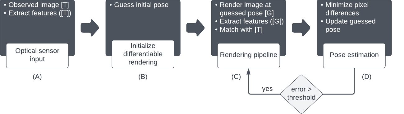
Figure 21: Flow of operations: Keypoint features from a reference image [T] image are extracted in stage (A) and an initial guess for pose is specified in (B). In (C), an image [G] is rendered with the guessed value of pose and matching features between [T] and [G] are identified. The pixel space difference between the matching features in [T] and [G] are iteratively minimized until convergence in the last two stages of operation.

Figure 21 illustrates the proposed differentiable rendering pipeline. Given a reference image consisting of an object of interest, the pipeline optimizes an initial guess for the six pose parameters to render an equivalent image. The pipeline of operations relies on establishing a correspondence between the reference [T] and the rendered [G] image pair. A sparse pixel correspondence is established based on SURF feature operator [91]. The features from the image pair are first matched, and the Euclidean distance between the pixels of the matched features is iteratively minimized using a nonlinear least squares approach. Here, the matched features need not be the same across iterations, but the algorithm relies on the matching of at least four features between the reference image and the image at the updated pose.

The NaRPA engine in the loop renders images at every updated pose value. The images are rendered using the 3D geometric model of the target object under study. As will be shown, the differentiable rendering problem solves for pose by solving a correspondence between 2D pixels and their respective 3D object coordinates. The 3D object coordinates are not assumed to be known apriori, but computed using 2D to 3D correspondence via stereopsis (Section 5.1). The correspondence may also be established from registration of point clouds generated by the NaRPA engine [92].

In the simulation paradigm, the ray tracer engine, generates these images (see Section 3.3) in rendering-time to deploy the pose estimation program at each event in the proximity maneuver. Utilizing the image feature data in 2D pixel as well as the 3D coordinates enables us to pose the differentiable rendering problem as a Perspective-n-Point Projection (PnP) problem [93] with $n$ number of tracked features. The idea is to formulate the PnP problem as an optimization problem with the objective to minimize the reprojection error of the target satellite’s image as seen by the camera on the spacecraft.

6.2 Image formation and the mathematical model of the PnP problem

Given n 3D reference points $\mathbf{a}_{i}=[x_{i}\;y_{i}\;z_{i}]^{T}$, $\textit{i}=1,2,...,n$, in an object reference frame, and their projections $\mathbf{b}_{i}=[x^{c}\;y^{c}\;z^{c}]^{T}$, in a camera’s view space, the PnP algorithm seeks to retrieve the proper orthogonal rotation matrix ${R}$ and the translation vector $\mathbf{t}$, that transform the points in the object reference frame to the view space. The projection transformation between the reference points and the corresponding view space coordinates is given by

$$\mathbf{b}_{i}=R\mathbf{a_{i}}+\mathbf{t},\;i=1,2,...n$$ (45)

where $R^{T}R=I$ and $\text{det}(R)=1$.

The perspective projection model extends the transformation in Eq. (45) from 3D view space coordinates to their corresponding 2D homogeneous image projections $\mathbf{p}_{i}=[u_{i}\;v_{i}\;1]^{T}$ for given intrinsic camera parameters as

$$s\mathbf{p}_{i}=K\>[R\;|\;\mathbf{t}]\,\mathbf{a}_{i}$$ (46)

where $s$ denotes the depth factor for the $i^{\text{th}}$ point and $K$ is the matrix of calibrated intrinsic camera parameters corresponding to axis skew $\gamma$, aspect ratio scaled focal lengths $(f_{x}$, $f_{y})$, and principal point offset $(x_{0},y_{0})$:

$$K=\begin{bmatrix}{f_{x}}&\gamma&x_{0}\\ 0&{f_{y}}&y_{0}\\ 0&0&1\end{bmatrix}$$ (47)

In this work, the attitude is represented using Gibbs or classical Rodrigues parameters (CRPs) [94, 95]. The CRPs facilitate posing the optimization problem via polynomial system solving, free of any trigonometric function. Let vector $\mathbf{q}=[q_{1}\;q_{2}\;q_{3}]^{T}$ denote the CRP, the rotation matrix $R$ in terms of $q$ can be obtained using Cayley transform as:

$$R=(I+[\mathbf{q}\times])^{-1}(I-[\mathbf{q}\times])$$ (48)

where $I\in{\rm I\!R}_{3\times 3}$ is an identity matrix, and operator $[\mathbf{q}\times]\in{\rm I\!R}_{3\times 3}$ converts a vector into a skew-symmetric matrix of the form:

$$[\mathbf{q}\times]=\begin{bmatrix}0&-q_{3}&q_{2}\\ q_{3}&0&-q_{1}\\ -q_{2}&q_{1}&0\end{bmatrix}$$ (49)

and

$$R=\frac{1}{1+\mathbf{q}^{T}\mathbf{q}}\begin{bmatrix}1+q_{1}^{2}-q_{2}^{2}-q_{3}^{2}&2(q_{1}q_{2}+q_{3})&2(q_{1}q_{3}-q_{2})\\ 2(q_{2}q_{1}-q_{3})&1-q_{1}^{2}+q_{2}^{2}-q_{3}^{2}&2(q_{2}q_{3}+q_{1})\\ 2(q_{3}q_{1}+q_{2})&2(q_{3}q_{2}-q_{1})&1+q_{1}^{2}-q_{2}^{2}-q_{3}^{2}\end{bmatrix}$$ (50)

Plugging the sensor specific parameters in Eq. (47), orientation matrix and translation vector in Eq. (50) into Eq. (46), we have the complete equation for the projection transformation in terms of the homography matrix $\mathbf{H}$:

$$s\begin{bmatrix}u_{i}\\ v_{i}\\ 1\end{bmatrix}=\begin{bmatrix}f&0&0\\ 0&f&0\\ 0&0&1\end{bmatrix}\begin{bmatrix}R_{11}&R_{12}&R_{13}&t_{1}\\ R_{21}&R_{22}&R_{23}&t_{2}\\ R_{31}&R_{32}&R_{33}&t_{3}\end{bmatrix}\begin{bmatrix}x_{i}\\ y_{i}\\ z_{i}\\ 1\end{bmatrix}$$ (51)

$$s\begin{bmatrix}u_{i}\\ v_{i}\\ 1\end{bmatrix}=\underbrace{\begin{bmatrix}h_{1}&h_{2}&h_{3}&h_{4}\\ h_{5}&h_{6}&h_{7}&h_{8}\\ h_{9}&h_{10}&h_{11}&h_{12}\end{bmatrix}}_{\mathbf{H}}\begin{bmatrix}x_{i}\\ y_{i}\\ z_{i}\\ 1\end{bmatrix}$$ (52)

Eq. (51) models the camera sensor configuration used in this exercise. The model assumes square pixels in the image sensor, zero skewness, and zero distortion. The homography matrix in Eq. (52) is the ultimate transformation between the 2D image projection points and the corresponding 3D reference points. Clearly, the projection points are rational evaluations of their corresponding 3D view points and are expressed as

$$u_{i}=\frac{h_{1}x_{i}+h_{2}y_{i}+h_{3}z_{i}+h_{4}}{s}$$ (53)

$$v_{i}=\frac{h_{5}x_{i}+h_{6}y_{i}+h_{7}z_{i}+h_{8}}{s}$$ (54)

where $s=h_{9}x_{i}+h_{10}y_{i}+h_{11}z_{i}+h_{12}$. The chirality condition [96] for the view geometry ensures that the depth factor $s$ is non-zero and on average, it is rigorously positive.

6.3 The minimization problem and iterative pose calculation

In this section, a nonlinear optimization approach for the calculation of pose parameters $\mathbf{x}=[q_{1}\;q_{2}\;q_{3}\;t_{1}\;t_{2}\;t_{3}]^{T}$ using Levenberg-Marquardt method is presented. Recall from Eqs. (51) and (52), the elements of the homography matrix are implicit functions of the pose parameters. Defining the function $\mathbf{g}(\mathbf{x}):\mathbb{R}^{6}\rightarrow\mathbb{R}^{12}$ to relate the set of pose parameters to the vector $\mathbf{h}$ with elements of the homography matrix $H$, and the function $\mathbf{f}(\mathbf{h}):\mathbb{R}^{12}\rightarrow\mathbb{R}^{2n}$ to map the intermediate variables in $\mathbf{h}$ to $n$ number of 2D image projections $\tilde{\mathbf{y}}$. Due to noise, Eq. (52) could not be satisfied in general. Therefore, we use an iterative nonlinear least squares optimization with the objective to minimize the reprojection error between the 2D image coordinates and the corresponding 3D reference points projected into the same image. The objective function for the minimization problem [97] is given as:

$$\min_{\mathbf{x}}||\tilde{\mathbf{y}}-\mathbf{f}(\mathbf{g}(\mathbf{x}))||_{2}^{2}=\sum_{i=0}^{n}\big{\{}(u_{i}-\mathbf{f}(\mathbf{g}(\mathbf{x}))^{2}+(v_{i}-\mathbf{f}(\mathbf{g}(\mathbf{x}))^{2}$$ (55)

Levenberg-Marquardt algorithm is used to iteratively estimate the pose parameters by refining the initial values until an optimal solution is obtained. The iterative procedure is represented as:

$${}\mathbf{x}_{i+1}=\mathbf{x}_{i}+\left(\mathbf{J}^{T}\mathbf{J}+\lambda\,\text{diag}(\mathbf{J}^{T}\mathbf{J})\right)^{-1}\mathbf{J}^{T}\mathbf{J}\big{(}\tilde{\mathbf{y}}-\mathbf{f}(\mathbf{g}(\mathbf{x}))\big{)}$$ (56)

where $\lambda$ is the LM update parameter and $\mathbf{J}\in\mathbb{R}^{2n\times 6}$ is the Jacobian matrix which includes the partial derivatives of the image formation model described in Sec. 6.2. $J$ is assembled from the individual Jacobians of the functions $f(h)$ and $g(x)$ using chain rule as explained in appendix [A]. The Levenberg-Marquardt variant implemented in this estimation exercise is delineated in appendix [B].

6.4 Results of differentiable rendering application

The proposed differentiable rendering technique is applied to an ISS docking maneuver application. Synthetic images are generated from a sequence of maneuvering steps in an ISS approach trajectory. The PnP based differentiable rendering is used to estimate the pose parameters from the known model of the ISS and the generated images using the proposed nonlinear optimization method (Eq. (56)). The images are synthesized at the estimated pose to visually validate the correctness of the algorithm. The error convergence of the pose estimation sequence are also plotted. The results of the said example application are shown in Fig. 22.

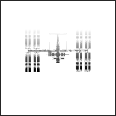
(a) Frame 1: True pose at $t_{1}$

(b) Frame 2: True pose at $t_{2}$

(c) Frame 3: True pose at $t_{3}$

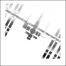
(d) Frame 4: True pose at $t_{4}$

(e) Frame 5: True pose at $t_{5}$

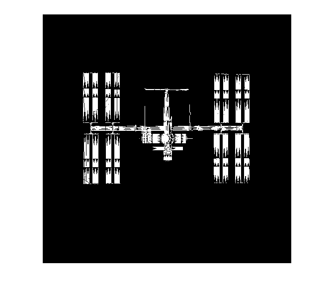
(f) Frame 1: Estimated pose at $t_{1}$

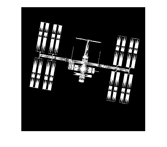
(g) Frame 2: Estimated pose at $t_{2}$

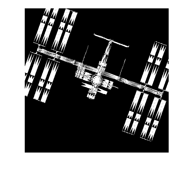
(h) Frame 3: Estimated pose at $t_{3}$

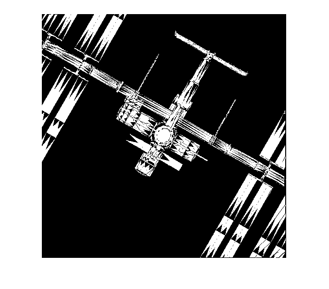
(i) Frame 4: Estimated pose at $t_{4}$

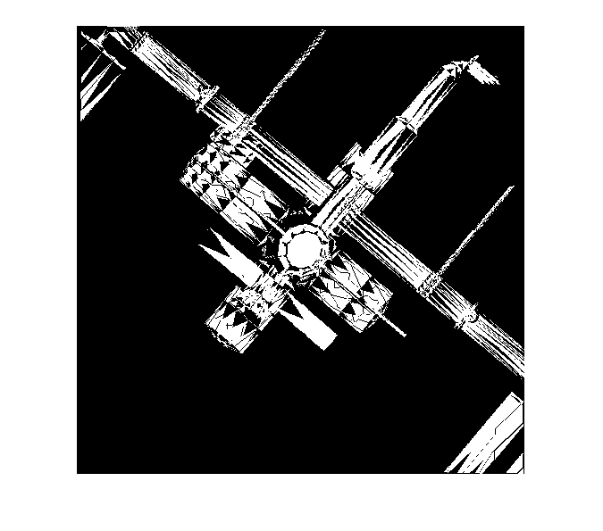
(j) Frame 5: Estimated pose at $t_{5}$

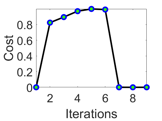
(k) Frame 1: Cost convergence

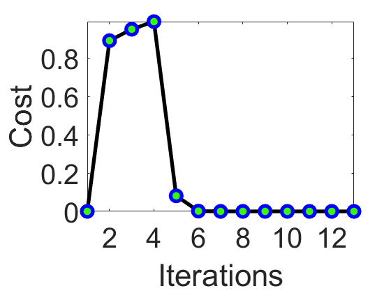
(l) Frame 2: Cost convergence

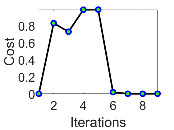
(m) Frame 3: Cost convergence

(n) Frame 4: Cost convergence

(o) Frame 5: Cost convergence

Figure 22: This figure illustrates the differentiable rendering based pose estimation for an ISS docking maneuver simulation. The top row indicates the true images synthesized from the true pose. The second row shows the images generated from the estimates of pose achieved from the differentiable rendering technique. The third row shows the convergence of cost function against the number of iterations in the nonlinear optimization.

7 Conclusion

In aerospace applications, testing and validation of vision-based navigation is governed by the ability to generate realistic simulations. Navigation and Rendering Pipeline for Astronautics (NaRPA) has been shown to generate physics inspired illumination models for virtual space missions. NaRPA is shown to have the capabilities to simulate space-to-space as well as ground-to-space observations that are sensitive to atmospheric scattering phenomena. With the capability to generate images, point clouds, depth, and contour maps, NaRPA is a multi-sensor simulation platform for future spacecraft missions.

This paper emphasizes the various capabilities of the NaRPA framework to imitate realistic observations. It is a ray-tracing based global illumination algorithm to account for a comprehensive nature of light propagation for photo-realism. The framework offers plugins to provide effects of time of day, turbidity, and exposure to include the atmospheric effects in the rendering process. To demonstrate the utility of NaRPA as a trustworthy simulation environment for vision-based navigation, two applications have been demonstrated.

In the first application, NaRPA is used as a stereo image generator for stereoscopic depth estimation. It is implemented as a tool for the verification of stereo vision algorithms, using the findings from a fundamental triangulation technique and point cloud data as ground truth. In the second application, a differentiable rendering algorithm is proposed for reasoning about 3D scenes from their corresponding 2D projections. In this application, relative pose is estimated from 3D scenes via nonlinear optimization by propagating gradients of the rendering process through the NaRPA simulations. Furthermore, using representative images and models, NaRPA is demonstrated to be of utility in testing and development of future guidance and navigation missions.

8 Acknowledgements

Drs. Carolina Restrepo (NASA-GSFC), Jerry Tessendorf (Clemson University), Daniel Crispell (Vision Systems Inc.), John Crassidis (University at Buffalo), Sarah Stevens (JPL), Anup Katake (JPL), Alejandro M San Martin (JPL), Nicolas Trawney (JPL), Eli D. Skulsky (JPL), Tejas Kulkarni (JPL), Daniel Crispell (VSI), Joe Mundy (VSI), Mr. Ronney Lovelace (NASA-JSC), and Mr. David van Wijk (Texas A&M) are acknowledged for their encouragement, guidance, and support in the development of NaRPA.

APPENDIX A Jacobian of the Image Formation Model

The image formation model represents a mapping from a 3D world scene to an image plane. This mapping is achieved by a set of intrinsic and extrinsic parameters that transform the scene points to the image plane (Eq. 52). The intrinsic parameters define the focal length and optical center of the imaging sensor, whereas the extrinsic parameters represent the position and orientation of the imaging sensor in the scene. Using homography matrix, Eqs. (53) and (54) (Section 6.2) relate the 3D scene coordinates to the image plane coordinates [97]. The function $\mathbf{f}(\mathbf{h}):\mathbb{R}^{12}\rightarrow\mathbb{R}^{2n}$ maps the elements, $h_{i}\in\mathbf{h}=\{h_{1},\ldots,h_{12}\}$, of the homography matrix to the image plane coordinates as

$$\mathbf{f}(\mathbf{h})=\begin{bmatrix}f_{1}(\mathbf{h})\\ f_{2}(\mathbf{h})\\ \vdots\\ f_{12}(\mathbf{h})\end{bmatrix}=\begin{bmatrix}u_{1}\\ v_{1}\\ \vdots\\ u_{n}\\ v_{n}\end{bmatrix}=\begin{bmatrix}\frac{h_{1}x_{1}+h_{2}y_{1}+h_{3}z_{1}+h_{4}}{h_{9}x_{1}+h_{10}y_{1}+h_{11}z_{1}+h_{12}}\\ \frac{h_{5}x_{1}+h_{6}y_{1}+h_{7}z_{1}+h_{8}}{h_{9}x_{1}+h_{10}y_{1}+h_{11}z_{1}+h_{12}}\\ \vdots\\ \frac{h_{1}x_{n}+h_{2}y_{n}+h_{3}z_{n}+h_{4}}{h_{9}x_{n}+h_{10}y_{n}+h_{11}z_{n}+h_{12}}\\ \frac{h_{5}x_{n}+h_{6}y_{n}+h_{7}z_{n}+h_{8}}{h_{9}x_{n}+h_{10}y_{n}+h_{11}z_{n}+h_{12}}\end{bmatrix}$$ (57)

Using Classical Rodrigues Parameters (CRPs) for attitude representation, the pose parameters $\mathbf{x}=[q_{1}\;q_{2}\;q_{3}\;t_{1}\;t_{2}\;t_{3}]^{T}$ are mapped to the homography matrix via a function $\mathbf{g}(\mathbf{x}):\mathbb{R}^{6}\rightarrow\mathbb{R}^{12}$ as

$$\mathbf{g}(\mathbf{x})=\begin{bmatrix}g_{1}(\mathbf{x})\\ g_{2}(\mathbf{x})\\ g_{3}(\mathbf{x})\\ g_{4}(\mathbf{x})\\ g_{5}(\mathbf{x})\\ g_{6}(\mathbf{x})\\ g_{7}(\mathbf{x})\\ g_{8}(\mathbf{x})\\ g_{9}(\mathbf{x})\\ g_{10}(\mathbf{x})\\ g_{11}(\mathbf{x})\\ g_{12}(\mathbf{x})\end{bmatrix}=\begin{bmatrix}h_{1}\\ h_{2}\\ h_{3}\\ h_{4}\\ h_{5}\\ h_{6}\\ h_{7}\\ h_{8}\\ h_{9}\\ h_{10}\\ h_{11}\\ h_{12}\end{bmatrix}=\frac{1}{1+q_{1}^{2}+q_{2}^{2}+q_{3}^{2}}\begin{bmatrix}1+q_{1}^{2}-q_{2}^{2}-q_{3}^{2}\\ 2(q_{1}q_{2}+q_{3})\\ 2(q_{1}q_{3}-q_{2})\\ t_{1}(1+q_{1}^{2}+q_{2}^{2}+q_{3}^{2})\\ 2(q_{2}q_{1}-q_{3})\\ 1-q_{1}^{2}+q_{2}^{2}-q_{3}^{2}\\ 2(q_{2}q_{3}+q_{1})\\ t_{2}(1+q_{1}^{2}+q_{2}^{2}+q_{3}^{2})\\ 2(q_{3}q_{1}+q_{2})\\ 2(q_{3}q_{2}-q_{1})\\ 1+q_{1}^{2}-q_{2}^{2}-q_{3}^{2}\\ t_{3}(1+q_{1}^{2}+q_{2}^{2}+q_{3}^{2})\end{bmatrix}$$ (58)

The equations (57) and (58) model the perspective projection transformation from 3D world coordinates to image plane coordinates. From the partial derivatives of $\mathbf{f}$ and $\mathbf{g}$, the Jacobian, $\mathbf{J}\in\mathbb{R}^{2n\times 6}$, of the image formation model is calculated using chain rule.

A.1 Partial Derivatives

The partial derivatives of $\mathbf{f}(\mathbf{h})$ and $\mathbf{g}(\mathbf{x})$, Jacobians $\mathbf{J}_{f}\in\mathbb{R}^{2n\times 12}$ and $\mathbf{J}_{g}\in\mathbb{R}^{2n\times 6}$ respectively, are computed below. The Jacobian $\mathbf{J}_{f}$ collects all first-order partial derivatives of the multivariate function $\mathbf{f}(\mathbf{h})$. The first row entries of $\mathbf{J}_{f}$ are

$$\frac{\partial f_{1}}{\partial h_{1}}=\frac{x_{1}}{h_{9}x_{1}+h_{10}y_{1}+h_{11}z_{1}+h_{12}},\qquad \frac{\partial f_{1}}{\partial h_{5}}=0,\qquad \frac{\partial f_{1}}{\partial h_{9}}=-\left(\frac{h_{1}x_{1}+h_{2}y_{1}+h_{3}z_{1}+h_{4}}{(h_{9}x_{1}+h_{10}y_{1}+h_{11}z_{1}+h_{12})^{2}}\right)x_{1},$$

$$\frac{\partial f_{1}}{\partial h_{2}}=\frac{y_{1}}{h_{9}x_{1}+h_{10}y_{1}+h_{11}z_{1}+h_{12}},\qquad \frac{\partial f_{1}}{\partial h_{6}}=0,\qquad \frac{\partial f_{1}}{\partial h_{10}}=-\left(\frac{h_{1}x_{1}+h_{2}y_{1}+h_{3}z_{1}+h_{4}}{(h_{9}x_{1}+h_{10}y_{1}+h_{11}z_{1}+h_{12})^{2}}\right)y_{1},$$

$$\frac{\partial f_{1}}{\partial h_{3}}=\frac{z_{1}}{h_{9}x_{1}+h_{10}y_{1}+h_{11}z_{1}+h_{12}},\qquad \frac{\partial f_{1}}{\partial h_{7}}=0,\qquad \frac{\partial f_{1}}{\partial h_{11}}=-\left(\frac{h_{1}x_{1}+h_{2}y_{1}+h_{3}z_{1}+h_{4}}{(h_{9}x_{1}+h_{10}y_{1}+h_{11}z_{1}+h_{12})^{2}}\right)z_{1},$$

$$\frac{\partial f_{1}}{\partial h_{4}}=\frac{1}{h_{9}x_{1}+h_{10}y_{1}+h_{11}z_{1}+h_{12}},\qquad \frac{\partial f_{1}}{\partial h_{8}}=0,\qquad \frac{\partial f_{1}}{\partial h_{12}}=-\left(\frac{h_{1}x_{1}+h_{2}y_{1}+h_{3}z_{1}+h_{4}}{(h_{9}x_{1}+h_{10}y_{1}+h_{11}z_{1}+h_{12})^{2}}\right)$$

The second row entries of $\mathbf{J}_{f}$ are

$$\frac{\partial f_{2}}{\partial h_{1}}=0,\qquad \frac{\partial f_{2}}{\partial h_{5}}=\frac{x_{1}}{h_{9}x_{1}+h_{10}y_{1}+h_{11}z_{1}+h_{12}},\qquad \frac{\partial f_{2}}{\partial h_{9}}=-\left(\frac{h_{1}x_{1}+h_{2}y_{1}+h_{3}z_{1}+h_{4}}{(h_{9}x_{1}+h_{10}y_{1}+h_{11}z_{1}+h_{12})^{2}}\right)x_{1},$$

$$\frac{\partial f_{2}}{\partial h_{2}}=0,\qquad \frac{\partial f_{2}}{\partial h_{6}}=\frac{y_{1}}{h_{9}x_{1}+h_{10}y_{1}+h_{11}z_{1}+h_{12}},\qquad \frac{\partial f_{2}}{\partial h_{10}}=-\left(\frac{h_{1}x_{1}+h_{2}y_{1}+h_{3}z_{1}+h_{4}}{(h_{9}x_{1}+h_{10}y_{1}+h_{11}z_{1}+h_{12})^{2}}\right)y_{1},$$

$$\frac{\partial f_{2}}{\partial h_{3}}=0,\qquad \frac{\partial f_{2}}{\partial h_{7}}=\frac{z_{1}}{h_{9}x_{1}+h_{10}y_{1}+h_{11}z_{1}+h_{12}},\qquad \frac{\partial f_{2}}{\partial h_{11}}=-\left(\frac{h_{1}x_{1}+h_{2}y_{1}+h_{3}z_{1}+h_{4}}{(h_{9}x_{1}+h_{10}y_{1}+h_{11}z_{1}+h_{12})^{2}}\right)z_{1},$$

$$\frac{\partial f_{2}}{\partial h_{4}}=0,\qquad \frac{\partial f_{2}}{\partial h_{8}}=\frac{1}{h_{9}x_{1}+h_{10}y_{1}+h_{11}z_{1}+h_{12}},\qquad \frac{\partial f_{2}}{\partial h_{12}}=-\left(\frac{h_{1}x_{1}+h_{2}y_{1}+h_{3}z_{1}+h_{4}}{(h_{9}x_{1}+h_{10}y_{1}+h_{11}z_{1}+h_{12})^{2}}\right)$$

Similarly, the partial derivatives of the remaining $10$ rows can be evaluated with only the coordinates $x_{i}$, $y_{i}$ to be adjusted in each row of $\mathbf{J}_{f}$.

The Jacobian $\mathbf{J}_{g}$ collects all first-order partial derivatives of the multivariate function $\mathbf{g}(\mathbf{h})$ that maps the pose parameters to the homography. The row-wise entries of $\mathbf{J}_{g}$ are as follows:

First row

$$\frac{\partial g_{1}}{\partial\mathbf{x}(1)}=\frac{4q_{1}(q_{2}^{2}+q_{3}^{2})}{(1+q_{1}^{2}+q_{2}^{2}+q_{3}^{2})^{2}},\qquad \frac{\partial g_{1}}{\partial\mathbf{x}(3)}=-\frac{4q_{3}(1+q_{1}^{2})}{(1+q_{1}^{2}+q_{2}^{2}+q_{3}^{2})^{2}},\qquad \frac{\partial g_{1}}{\partial\mathbf{x}(5)}=0,$$

$$\frac{\partial g_{1}}{\partial\mathbf{x}(2)}=-\frac{4q_{2}(1+q_{1}^{2})}{(1+q_{1}^{2}+q_{2}^{2}+q_{3}^{2})^{2}},\qquad \frac{\partial g_{1}}{\partial\mathbf{x}(4)}=0,\qquad \frac{\partial g_{1}}{\partial\mathbf{x}(6)}=0$$

second row

$$\frac{\partial g_{2}}{\partial\mathbf{x}(1)}=\frac{2(q_{2}+q_{2}q_{3}^{2}+q_{2}^{3}-2q_{1}q_{3}-q_{1}^{2}q_{2})}{(1+q_{1}^{2}+q_{2}^{2}+q_{3}^{2})^{2}},\qquad \frac{\partial g_{2}}{\partial\mathbf{x}(3)}=\frac{2(q_{1}^{2}-2q_{1}q_{2}q_{3}+q_{2}^{2}-q_{3}^{2}+1)}{(1+q_{1}^{2}+q_{2}^{2}+q_{3}^{2})^{2}},\qquad \frac{\partial g_{2}}{\partial\mathbf{x}(5)}=0,$$

$$\frac{\partial g_{2}}{\partial\mathbf{x}(2)}=\frac{2(q_{1}^{3}-q_{1}q_{2}^{2}+q_{1}q_{3}^{2}+q_{1}-2q_{2}q_{3})}{(1+q_{1}^{2}+q_{2}^{2}+q_{3}^{2})^{2}},\qquad \frac{\partial g_{2}}{\partial\mathbf{x}(4)}=0,\qquad \frac{\partial g_{2}}{\partial\mathbf{x}(6)}=0$$

third row

$$\frac{\partial g_{3}}{\partial\mathbf{x}(1)}=\frac{2(q_{3}+q_{3}^{3}+q_{2}^{2}q_{3}+2q_{1}q_{2}-q_{1}^{2}q_{3})}{(1+q_{1}^{2}+q_{2}^{2}+q_{3}^{2})^{2}},\qquad \frac{\partial g_{3}}{\partial\mathbf{x}(3)}=\frac{2(q_{1}^{3}+q_{1}q_{2}^{2}-q_{1}q_{3}^{2}+q_{1}+2q_{2}q_{3})}{(1+q_{1}^{2}+q_{2}^{2}+q_{3}^{2})^{2}},\qquad \frac{\partial g_{3}}{\partial\mathbf{x}(5)}=0,$$

$$\frac{\partial g_{3}}{\partial\mathbf{x}(2)}=-\frac{2(q_{1}^{2}+2q_{1}q_{2}q_{3}-q_{2}^{2}+q_{3}^{2}+1)}{(1+q_{1}^{2}+q_{2}^{2}+q_{3}^{2})^{2}},\qquad \frac{\partial g_{3}}{\partial\mathbf{x}(4)}=0,\qquad \frac{\partial g_{3}}{\partial\mathbf{x}(6)}=0$$

fourth row

$$\frac{\partial g_{4}}{\partial\mathbf{x}(1)}=0,\qquad \frac{\partial g_{4}}{\partial\mathbf{x}(3)}=0,\qquad \frac{\partial g_{4}}{\partial\mathbf{x}(5)}=0,$$

$$\frac{\partial g_{4}}{\partial\mathbf{x}(2)}=0,\qquad \frac{\partial g_{4}}{\partial\mathbf{x}(4)}=1,\qquad \frac{\partial g_{4}}{\partial\mathbf{x}(6)}=0$$

fifth row

$$\frac{\partial g_{5}}{\partial\mathbf{x}(1)}=\frac{2(-q_{1}^{2}q_{2}+2q_{1}q_{3}+q_{2}^{3}+q_{2}q_{3}^{2}+q_{2})}{(1+q_{1}^{2}+q_{2}^{2}+q_{3}^{2})^{2}},\qquad \frac{\partial g_{5}}{\partial\mathbf{x}(3)}=-\frac{2(q_{1}^{2}+2q_{1}q_{2}q_{3}+q_{2}^{2}-q_{3}^{2}+1)}{(1+q_{1}^{2}+q_{2}^{2}+q_{3}^{2})^{2}},\qquad \frac{\partial g_{5}}{\partial\mathbf{x}(5)}=0,$$

$$\frac{\partial g_{5}}{\partial\mathbf{x}(2)}=\frac{2(q_{1}^{3}-q_{1}q_{2}^{2}+q_{1}q_{3}^{2}+q_{1}+2q_{2}q_{3})}{(1+q_{1}^{2}+q_{2}^{2}+q_{3}^{2})^{2}},\qquad \frac{\partial g_{5}}{\partial\mathbf{x}(4)}=0,\qquad \frac{\partial g_{5}}{\partial\mathbf{x}(6)}=0$$

sixth row

$$\frac{\partial g_{6}}{\partial\mathbf{x}(1)}=-\frac{4q_{1}(q_{2}^{2}+1)}{(1+q_{1}^{2}+q_{2}^{2}+q_{3}^{2})^{2}},\qquad \frac{\partial g_{6}}{\partial\mathbf{x}(3)}=-\frac{4q_{3}(q_{2}^{2}+1)}{(1+q_{1}^{2}+q_{2}^{2}+q_{3}^{2})^{2}},\qquad \frac{\partial g_{6}}{\partial\mathbf{x}(5)}=0,$$

$$\frac{\partial g_{6}}{\partial\mathbf{x}(2)}=\frac{4q_{2}(q_{1}^{2}+q_{3}^{2})}{(1+q_{1}^{2}+q_{2}^{2}+q_{3}^{2})^{2}},\qquad \frac{\partial g_{6}}{\partial\mathbf{x}(4)}=0,\qquad \frac{\partial g_{6}}{\partial\mathbf{x}(6)}=0$$

seventh row

$$\frac{\partial g_{7}}{\partial\mathbf{x}(1)}=\frac{2(-q_{1}^{2}-2q_{1}q_{2}q_{3}+q_{2}^{2}+q_{3}^{2}+1)}{(1+q_{1}^{2}+q_{2}^{2}+q_{3}^{2})^{2}},\qquad \frac{\partial g_{7}}{\partial\mathbf{x}(3)}=\frac{2(q_{1}^{2}q_{2}-2q_{1}q_{3}+q_{2}^{3}-q_{2}q_{3}^{2}+q_{2})}{(1+q_{1}^{2}+q_{2}^{2}+q_{3}^{2})^{2}},\qquad \frac{\partial g_{7}}{\partial\mathbf{x}(5)}=0,$$

$$\frac{\partial g_{7}}{\partial\mathbf{x}(2)}=\frac{2(q_{1}^{2}q_{3}-2q_{1}q_{2}-q_{2}^{2}q_{3}+q_{3}^{3}+q_{3})}{(1+q_{1}^{2}+q_{2}^{2}+q_{3}^{2})^{2}},\qquad \frac{\partial g_{7}}{\partial\mathbf{x}(4)}=0,\qquad \frac{\partial g_{7}}{\partial\mathbf{x}(6)}=0$$

eighth row

$$\frac{\partial g_{8}}{\partial\mathbf{x}(1)}=0,\qquad \frac{\partial g_{8}}{\partial\mathbf{x}(3)}=0,\qquad \frac{\partial g_{8}}{\partial\mathbf{x}(5)}=1,$$

$$\frac{\partial g_{8}}{\partial\mathbf{x}(2)}=0,\qquad \frac{\partial g_{8}}{\partial\mathbf{x}(4)}=0,\qquad \frac{\partial g_{8}}{\partial\mathbf{x}(6)}=0$$

ninth row

$$\frac{\partial g_{9}}{\partial\mathbf{x}(1)}=\frac{2(-q_{1}^{2}q_{3}-2q_{1}q_{2}+q_{2}^{2}q_{3}+q_{3}^{3}+q_{3})}{(1+q_{1}^{2}+q_{2}^{2}+q_{3}^{2})^{2}},\quad \frac{\partial g_{9}}{\partial\mathbf{x}(3)}=-\frac{2(q_{1}^{3}+q_{1}q_{2}^{2}-q_{1}q_{3}^{2}+q_{1}-2q_{2}q_{3})}{(1+q_{1}^{2}+q_{2}^{2}+q_{3}^{2})^{2}},\quad \frac{\partial g_{9}}{\partial\mathbf{x}(5)}=0,$$

$$\frac{\partial g_{9}}{\partial\mathbf{x}(2)}=\frac{2(q_{1}^{2}-2q_{1}q_{2}q_{3}-q_{2}^{2}+q_{3}^{2}+1)}{(1+q_{1}^{2}+q_{2}^{2}+q_{3}^{2})^{2}},\quad \frac{\partial g_{9}}{\partial\mathbf{x}(4)}=0,\quad \frac{\partial g_{9}}{\partial\mathbf{x}(6)}=0$$

tenth row

$$\frac{\partial g_{10}}{\partial\mathbf{x}(1)}=\frac{-2(-q_{1}^{2}+2q_{1}q_{2}q_{3}+q_{2}^{2}+q_{3}^{2}+1)}{(1+q_{1}^{2}+q_{2}^{2}+q_{3}^{2})^{2}},\quad \frac{\partial g_{10}}{\partial\mathbf{x}(3)}=\frac{2(q_{1}^{2}q_{2}+2q_{1}q_{3}+q_{2}^{3}-q_{2}q_{3}^{2}+q_{2})}{(1+q_{1}^{2}+q_{2}^{2}+q_{3}^{2})^{2}},\quad \frac{\partial g_{10}}{\partial\mathbf{x}(5)}=0,$$

$$\frac{\partial g_{10}}{\partial\mathbf{x}(2)}=\frac{2(q_{1}^{2}q_{3}+2q_{1}q_{2}-q_{2}^{2}q_{3}+q_{3}^{3}+q_{3})}{(1+q_{1}^{2}+q_{2}^{2}+q_{3}^{2})^{2}},\quad \frac{\partial g_{10}}{\partial\mathbf{x}(4)}=0,\quad \frac{\partial g_{10}}{\partial\mathbf{x}(6)}=0$$

eleventh row

$$\frac{\partial g_{11}}{\partial\mathbf{x}(1)}=\frac{-4q_{1}(q_{3}^{2}+1)}{(1+q_{1}^{2}+q_{2}^{2}+q_{3}^{2})^{2}},\qquad \frac{\partial g_{11}}{\partial\mathbf{x}(3)}=\frac{4q_{3}(q_{1}^{2}+q_{2}^{2})}{(1+q_{1}^{2}+q_{2}^{2}+q_{3}^{2})^{2}},\qquad \frac{\partial g_{11}}{\partial\mathbf{x}(5)}=0,$$

$$\frac{\partial g_{11}}{\partial\mathbf{x}(2)}=\frac{-4q_{2}(q_{3}^{2}+1))}{(1+q_{1}^{2}+q_{2}^{2}+q_{3}^{2})^{2}},\qquad \frac{\partial g_{11}}{\partial\mathbf{x}(4)}=0,\qquad \frac{\partial g_{11}}{\partial\mathbf{x}(6)}=0$$

and the twelfth row

$$\frac{\partial g_{12}}{\partial\mathbf{x}(1)}=0,\qquad \frac{\partial g_{12}}{\partial\mathbf{x}(3)}=0,\qquad \frac{\partial g_{12}}{\partial\mathbf{x}(5)}=0,$$

$$\frac{\partial g_{12}}{\partial\mathbf{x}(2)}=0,\qquad \frac{\partial g_{12}}{\partial\mathbf{x}(4)}=0,\qquad \frac{\partial g_{12}}{\partial\mathbf{x}(6)}=1$$

Finally, with the individual Jacobians $\mathbf{J}(\mathbf{f})$ and $\mathbf{J}(\mathbf{g})$, the Jacobian of the image formation model, $\mathbf{J}$, can be assembled using chain rule as

$$\frac{\partial}{\partial\mathbf{x}}\mathbf{f}(\mathbf{g}(\mathbf{x}))=\mathbf{J}=\mathbf{J}_{f}\cdot\mathbf{J}_{g}={\begin{bmatrix}\frac{\partial f_{1}}{\partial h_{1}}&\ldots&\frac{\partial f_{1}}{\partial h_{12}}\\ \vdots&\ddots&\vdots\\ \frac{\partial f_{12}}{\partial h_{1}}&\ldots&\frac{\partial f_{12}}{\partial h_{12}}\end{bmatrix}}_{12\times 12}{\begin{bmatrix}\frac{\partial g_{1}}{\partial\mathbf{x}(1)}&\ldots&\frac{\partial g_{1}}{\partial\mathbf{x}(6)}\\ \vdots&\ddots&\vdots\\ \frac{\partial g_{12}}{\partial\mathbf{x}(1)}&\ldots&\frac{\partial f_{12}}{\partial\mathbf{x}(6)}\end{bmatrix}}_{12\times 6}$$ (59)

APPENDIX B Levenberg-Marquardt Method For Nonlinear Least Squares

The Levenberg-Marquardt (LM) algorithm [98] is an iterative technique to solve nonlinear least squares optimization problems. The LM method blends two numerical minimization problems: the gradient descent method and the Gauss-Newton method. The gradient descent approach updates the parameters in the steepest direction of descent and helps reach a function minimum in a very few iterations, even when the initial guess is far away from the optimum. However, its behavior is sluggish when near the optimum point. On the other hand, the Gauss-Newton method solves for the minimum of a function that is assumed to be a locally quadratic model. In contrary to gradient descent, the Gauss-Newton method may not converge if the initial guess is far from the optimum and shows a faster convergence when near it. The LM method combines the advantages of gradient descent and Newton’s methods in which it adapts gradient-descent method when parameters are far from the optimum, and Gauss-Newton technique when the parameters are close to the optimum point.

Formulation of the Levenberg-Marquardt Method

Let us consider a nonlinear function $\mathbf{f}$ that maps a parameter vector $\mathbf{p}\in\mathbb{R}^{m}$ to an estimated measurement vector $\hat{\mathbf{y}}$ through the relation $\hat{\mathbf{y}}=\mathbf{f(p)}$, where $\hat{\mathbf{y}}\in\mathbb{R}^{n}$. Provided an initial parameter $\mathbf{p_{0}}$ and a measurement vector $\tilde{\mathbf{y}}$, we seek the estimate ($\mathbf{\hat{p}}$) for $\mathbf{p}$ that minimizes the squared error ($||\mathbf{e}||^{2}$) between the measured and the evaluated values of the nonlinear function $\mathbf{f}$

$$\min_{\mathbf{\hat{\mathbf{p}}}\in\mathbb{R}^{n}}\chi^{2}(\hat{\mathbf{p}})={||\mathbf{e}||^{2}}_{W}=[\mathbf{\tilde{y}}-\mathbf{f(\hat{\mathbf{p}})}]^{T}W[\mathbf{\tilde{y}}-\mathbf{f(\hat{\mathbf{p}})}]$$ (60)

A linear approximation of $\mathbf{f}$ in the neighborhood of $\mathbf{\hat{\mathbf{p}}}$, from the Taylor series expansion results in the approximation

$$\mathbf{f(p+h)}\approx\mathbf{f(p)+Jh}$$ (61)

where $\mathbf{J}$ is the Jacobian of $\mathbf{f}$ i.e., $\mathbf{J}=\frac{\partial\mathbf{f(p)}}{\partial\mathbf{p}}$.

The LM method is an iterative procedure that at each iteration computes a step $\mathbf{h}$ as a solution of the linearized least-squares sub-problem:

$$\min_{\mathbf{h}\in\mathbb{R}^{n}}m_{i}(\mathbf{p})={||\mathbf{\tilde{y}}-\mathbf{f(p)}-\mathbf{Jh}||^{2}}_{W}$$ (62)

In the LM method, it is required to find a $\mathbf{h}$ that minimizes the quantity $||\mathbf{\tilde{y}}-\mathbf{f(p+h)}||\approx||\mathbf{\tilde{y}}-\mathbf{f(p)}-\mathbf{Jh}||=||\mathbf{e}-\mathbf{Jh}||$. The least squares algorithm yields $\mathbf{h}$ as the solution of

$$\mathbf{J^{T}}\mathbf{WJh}=\mathbf{J}^{T}\mathbf{W(\tilde{y}-\hat{y})}$$ (63)

The solution from LM method is a slight variation of Eq. (63),

$$[\mathbf{J}^{T}\mathbf{WJ}+\lambda\mathbf{I}]\mathbf{h_{lm}}=\mathbf{J}^{T}\mathbf{W(\tilde{y}-\hat{y})}$$ (64)

This solution introduces a damping term $\lambda$ which adaptively modifies the method of optimization across each iteration. If the updated parameter vector $\mathbf{p+h}$ leads to a reduction in error $\mathbf{e}$, the update is accepted and the process moves on to the next iteration with a decreased $\lambda$. If any iteration results in an increase in error, $\lambda$ is increased to find a $\mathbf{h}$ that decreases the error. The initial updates are ensured in the steepest-descent direction by initializing the damping term $\lambda$ appropriately large. As the solution improves towards a minimum, the $\lambda$ is decreased, and the LM update step approaches the Newton’s method. Further, the $\lambda$’s are normalized to the values of $\mathbf{J}^{T}\mathbf{WJ}$ to fine-tune the scaling

$$[\mathbf{J}^{T}\mathbf{WJ}+\lambda\,\text{diag}(\mathbf{J}^{T}\mathbf{WJ})]=\mathbf{J}^{T}\mathbf{W(\tilde{y}-\hat{y})}$$ (65)

The objective of the optimization problem is to find an estimated measurement vector, $\mathbf{\hat{y}}$ is such that it reduces the squared distance $\epsilon^{T}\epsilon$ with $\epsilon$ being equal to $\mathbf{y-\hat{y}}$.

Updating the damping term $\lambda$

The method adopted for updating $\lambda$ is as follows. At each iteration i, if a step $\mathbf{h}$ sufficiently decreases the objective function, it is accepted, and the algorithm proceeds to the next iteration. Otherwise, the step is rejected, $\lambda_{i}$ is updated, and the minimization problem is solved again. A gain metric $\rho_{i}(\mathbf{h})$ shown in Eq. (68) helps evaluate a ratio between actual and predicted reduction in objective function

$$\rho(\mathbf{h}_{lm})=\frac{\chi^{2}(\mathbf{p})-\chi^{2}(\mathbf{p}+\mathbf{h}_{lm})}{m_{i}(\mathbf{p})-m_{i}(\mathbf{p}+\mathbf{h}_{lm})}$$ (66)

where,

$$m_{i}(\mathbf{p})-m_{i}(\mathbf{p}+\mathbf{h}_{lm}) =\mathbf{h}_{lm}^{T}(\lambda_{i}\text{diag}(\mathbf{J}^{T}\mathbf{WJ})\mathbf{h}_{lm}+\mathbf{J}^{T}\mathbf{W}(\mathbf{y}-\hat{\mathbf{y}}{(\mathbf{p})}))$$ (67)

such that

$$\rho(\mathbf{h}_{lm})=\frac{\chi^{2}(\mathbf{p})-\chi^{2}(\mathbf{p}+\mathbf{h}_{lm})}{\mathbf{h}_{lm}^{T}[\lambda_{i}\text{diag}(\mathbf{J}^{T}\mathbf{WJ})\mathbf{h}_{lm}+\mathbf{J}^{T}\mathbf{W}(\mathbf{y}-{\hat{\mathbf{y}}(\mathbf{p})})]}$$ (68)

By construction, the denominator is a positive quantity, and $\rho_{i}>0$ is equivalent to the minimizing step direction. The step $h_{lm}$ is accepted if the metric $\rho_{i}$ is greater than a user-specified threshold, $\epsilon>0$. If an iteration results in $\rho_{i}>\epsilon$, then the step resulted in a decrease in objective function, and we update the parameter $\mathbf{p}$ to $\mathbf{p}+\mathbf{h}$, and then reduce the damping term $\lambda_{i}$ by a factor. If gain $\rho_{i}$ is a smaller value than $\epsilon$, it indicates that we should increase the damping term and thereby increase the penalty on large steps before proceeding to the next iteration.

1 Compute the $\chi^{2}$ objective function from the user-specified starting value of $\lambda_{0}$, initial guessed parameter vector $\mathbf{p}$, nonlinear function $\mathbf{f}$ and measurement data $\mathbf{\tilde{y}}$

2 Compute $\mathbf{h}_{lm}$ and $\rho_{i}(\mathbf{h}_{lm})$ using the equations:

$$\mathbf{h_{lm}} =[\mathbf{J}^{T}\mathbf{WJ}+\lambda\mathbf{I}]^{-1}\mathbf{J}^{T}\mathbf{W(\tilde{y}-\hat{y})}$$

$$\rho(\mathbf{h}_{lm}) =\frac{\chi^{2}(\mathbf{p})-\chi^{2}(\mathbf{p}+\mathbf{h}_{lm})}{\mathbf{h}_{lm}^{T}[\lambda_{i}\text{diag}(\mathbf{J}^{T}\mathbf{WJ})\mathbf{h}_{lm}+\mathbf{J}^{T}\mathbf{W}(\mathbf{y}-{\hat{\mathbf{y}}(\mathbf{p})})]}$$

If $\rho_{i}(\mathbf{h}_{lm})>\epsilon$: $\mathbf{p}\leftarrow\mathbf{p}+\mathbf{h}$; $\lambda_{i+1}=max[\lambda_{i}/L_{\downarrow},10^{-7}]$;
otherwise: $\lambda_{i+1}=min[\lambda_{i}/L_{\uparrow},10^{7}]$

$[L_{\uparrow},L_{\downarrow}]=[10,10]$ are the factors chosen in this paper for updating the damping term.

Algorithm 1 Levenberg-Marquardt Method

References

- Johnson et al. [2007] Johnson, A., Ansar, A., Matthies, L., Trawny, N., Mourikis, A., and Roumeliotis, S., “A general approach to terrain relative navigation for planetary landing,” AIAA Infotech@ Aerospace 2007 Conference and Exhibit, 2007, p. 2854.
- McCabe and DeMars [2020] McCabe, J. S., and DeMars, K. J., “Anonymous feature-based terrain relative navigation,” Journal of Guidance, Control, and Dynamics, Vol. 43, No. 3, 2020, pp. 410–421.
- Adams et al. [2008] Adams, D., Criss, T. B., and Shankar, U. J., “Passive optical terrain relative navigation using APLNav,” 2008 ieee aerospace conference, IEEE, 2008, pp. 1–9.
- Michaelis et al. [2017] Michaelis, H., Behnke, T., Bredthauer, R., Holland, A., Janesick, J., Jaumann, R., Keller, H., Magrin, D., Greggio, D., Mottola, S., et al., “Planetary exploration with optical imaging systems review: what is the best sensor for future missions,” International Conference on Space Optics—ICSO 2014, Vol. 10563, International Society for Optics and Photonics, 2017, p. 1056322.
- Benninghoff et al. [2014] Benninghoff, H., Boge, T., and Rems, F., “Autonomous navigation for on-orbit servicing,” KI-Künstliche Intelligenz, Vol. 28, No. 2, 2014, pp. 77–83.
- Zhang et al. [2008] Zhang, G., Liu, H., Wang, J., and Jiang, Z., “Vision-based system for satellite on-orbit self-servicing,” 2008 IEEE/ASME International Conference on Advanced Intelligent Mechatronics, IEEE, 2008, pp. 296–301.
- Kelsey et al. [2006] Kelsey, J. M., Byrne, J., Cosgrove, M., Seereeram, S., and Mehra, R. K., “Vision-based relative pose estimation for autonomous rendezvous and docking,” 2006 IEEE aerospace conference, IEEE, 2006, pp. 20–pp.
- Aghili et al. [2010] Aghili, F., Kuryllo, M., Okouneva, G., and English, C., “Robust vision-based pose estimation of moving objects for automated rendezvous & docking,” 2010 IEEE International Conference on Mechatronics and Automation, IEEE, 2010, pp. 305–311.
- Petit et al. [2011] Petit, A., Marchand, E., and Kanani, K., “Vision-based space autonomous rendezvous: A case study,” 2011 IEEE/RSJ International Conference on Intelligent Robots and Systems, IEEE, 2011, pp. 619–624.
- Liu and Hu [2014] Liu, C., and Hu, W., “Relative pose estimation for cylinder-shaped spacecrafts using single image,” IEEE Transactions on Aerospace and Electronic Systems, Vol. 50, No. 4, 2014, pp. 3036–3056.
- Cropp et al. [2000] Cropp, A., Palmer, P., McLauchlan, P., and Underwood, C., “Estimating pose of known target satellite,” Electronics Letters, Vol. 36, No. 15, 2000, pp. 1331–1332.
- Abderrahim et al. [2005] Abderrahim, M., Diaz, J., Rossi, C., and Salichs, M., “Experimental simulation of satellite relative navigation using computer vision,” Proceedings of 2nd International Conference on Recent Advances in Space Technologies, 2005. RAST 2005., IEEE, 2005, pp. 379–384.
- Du et al. [2009] Du, X., Liang, B., and Tao, Y., “Pose determination of large non-cooperative satellite in close range using coordinated cameras,” 2009 International Conference on Mechatronics and Automation, IEEE, 2009, pp. 3910–3915.
- Segal et al. [2011] Segal, S., Carmi, A., and Gurfil, P., “Vision-based relative state estimation of non-cooperative spacecraft under modeling uncertainty,” 2011 Aerospace Conference, IEEE, 2011, pp. 1–8.
- Zhang et al. [2013] Zhang, H., Jiang, Z., and Elgammal, A., “Vision-based pose estimation for cooperative space objects,” Acta Astronautica, Vol. 91, 2013, pp. 115–122.
- Zhang et al. [2015] Zhang, H., Jiang, Z., and Elgammal, A., “Satellite recognition and pose estimation using homeomorphic manifold analysis,” IEEE Transactions on Aerospace and Electronic Systems, Vol. 51, No. 1, 2015, pp. 785–792.
- Opromolla et al. [2017] Opromolla, R., Fasano, G., Rufino, G., and Grassi, M., “Pose estimation for spacecraft relative navigation using model-based algorithms,” IEEE Transactions on Aerospace and Electronic Systems, Vol. 53, No. 1, 2017, pp. 431–447.
- Xu and Kanade [1992] Xu, Y., and Kanade, T., Space robotics: dynamics and control, Vol. 188, Springer Science & Business Media, 1992.
- Nishida et al. [2009] Nishida, S.-I., Kawamoto, S., Okawa, Y., Terui, F., and Kitamura, S., “Space debris removal system using a small satellite,” Acta Astronautica, Vol. 65, No. 1-2, 2009, pp. 95–102.
- Forshaw et al. [2016] Forshaw, J. L., Aglietti, G. S., Navarathinam, N., Kadhem, H., Salmon, T., Pisseloup, A., Joffre, E., Chabot, T., Retat, I., Axthelm, R., et al., “RemoveDEBRIS: An in-orbit active debris removal demonstration mission,” Acta Astronautica, Vol. 127, 2016, pp. 448–463.
- Junkins and Strikwerda [1979] Junkins, J., and Strikwerda, T., “Autonomous attitude estimation via star sensing and pattern recognition,” NASA. Goddard Space Flight Center Flight Mech.(Estimation Theory Symp., 1979.
- Spratling and Mortari [2009] Spratling, B. B., and Mortari, D., “A survey on star identification algorithms,” Algorithms, Vol. 2, No. 1, 2009, pp. 93–107.
- Gnam et al. [2019] Gnam, C., Liounis, A., Ashman, B., Getzandanner, K., Lyzhoft, J., Small, J., Highsmith, D., Adam, C., Leonard, J., Antreasian, P., et al., “A Novel Surface Feature Navigation Algorithm Using Ray Tracing,” RPI Space Imaging Workshop, 2019.
- Glassner [1989] Glassner, A. S., An introduction to ray tracing, Morgan Kaufmann, 1989.
- Hughes et al. [2014] Hughes, J. F., Van Dam, A., McGuire, M., Foley, J. D., Sklar, D., Feiner, S. K., and Akeley, K., Computer graphics: principles and practice, Pearson Education, 2014.
- Shreiner et al. [2013] Shreiner, D., Sellers, G., Kessenich, J., and Licea-Kane, B., OpenGL programming guide: The Official guide to learning OpenGL, version 4.3, Addison-Wesley, 2013.
- Corporation [2003] Corporation, M., Microsoft DirectX 9 programmable graphics pipeline, Microsoft Press, 2003.
- Davidovič et al. [2012] Davidovič, T., Engelhardt, T., Georgiev, I., Slusallek, P., and Dachsbacher, C., “3D rasterization: a bridge between rasterization and ray casting,” Proceedings of Graphics Interface 2012, 2012, pp. 201–208.
- Whitted [1979] Whitted, T., “An improved illumination model for shaded display,” Proceedings of the 6th annual conference on Computer graphics and interactive techniques, 1979, p. 14.
- Cook et al. [1984] Cook, R. L., Porter, T., and Carpenter, L., “Distributed ray tracing,” Proceedings of the 11th annual conference on Computer graphics and interactive techniques, 1984, pp. 137–145.
- Kajiya [1986] Kajiya, J. T., “The rendering equation,” Proceedings of the 13th annual conference on Computer graphics and interactive techniques, 1986, pp. 143–150.
- Goral et al. [1984] Goral, C. M., Torrance, K. E., Greenberg, D. P., and Battaile, B., “Modeling the interaction of light between diffuse surfaces,” ACM SIGGRAPH computer graphics, Vol. 18, No. 3, 1984, pp. 213–222.
- Cohen and Greenberg [1985] Cohen, M. F., and Greenberg, D. P., “The hemi-cube: A radiosity solution for complex environments,” ACM Siggraph Computer Graphics, Vol. 19, No. 3, 1985, pp. 31–40.
- Nishita and Nakamae [1985] Nishita, T., and Nakamae, E., “Continuous tone representation of three-dimensional objects taking account of shadows and interreflection,” ACM SIGGRAPH Computer Graphics, Vol. 19, No. 3, 1985, pp. 23–30.
- Lafortune and Willems [1996] Lafortune, E. P., and Willems, Y. D., “Rendering Participating Media with Bidirectional Path Tracing,” Rendering Techniques ’96, edited by X. Pueyo and P. Schröder, Springer Vienna, Vienna, 1996, pp. 91–100.
- Veach and Guibas [1997] Veach, E., and Guibas, L. J., “Metropolis light transport,” Proceedings of the 24th annual conference on Computer graphics and interactive techniques, 1997, pp. 65–76.
- Ward et al. [1988] Ward, G. J., Rubinstein, F. M., and Clear, R. D., “A ray tracing solution for diffuse interreflection,” Proceedings of the 15th annual conference on Computer graphics and interactive techniques, 1988, pp. 85–92.
- Jensen [2001] Jensen, H. W., Realistic image synthesis using photon mapping, AK Peters/CRC Press, 2001.
- Wald et al. [2001] Wald, I., Slusallek, P., and Benthin, C., “Interactive distributed ray tracing of highly complex models,” Eurographics Workshop on Rendering Techniques, Springer, 2001, pp. 277–288.
- Parker et al. [2013] Parker, S. G., Friedrich, H., Luebke, D., Morley, K., Bigler, J., Hoberock, J., McAllister, D., Robison, A., Dietrich, A., Humphreys, G., et al., “GPU ray tracing,” Communications of the ACM, Vol. 56, No. 5, 2013, pp. 93–101.
- Ward [1994] Ward, G. J., “The RADIANCE lighting simulation and rendering system,” Proceedings of the 21st annual conference on Computer graphics and interactive techniques, 1994, pp. 459–472.
- Glassner [1993] Glassner, A., “Spectrum: An architecture for image synthesis, research, education, and practice,” Developing Large-scale Graphics Software Toolkits,(SIGGRAPH’93 Course Notes 3), pages, 1993, pp. 1–1.
- Slusallek and Seidel [1995] Slusallek, P., and Seidel, H.-P., “Vision-an architecture for global illumination calculations,” IEEE Transactions on Visualization and Computer Graphics, Vol. 1, No. 1, 1995, pp. 77–96.
- Pharr et al. [2016] Pharr, M., Jakob, W., and Humphreys, G., Physically based rendering: From theory to implementation, Morgan Kaufmann, 2016.
- Plachetka [1998] Plachetka, T., “POV Ray: persistence of vision parallel raytracer,” Proc. of Spring Conf. on Computer Graphics, Budmerice, Slovakia, Vol. 123, 1998, p. 129.
- Iraci [2013] Iraci, B., Blender cycles: lighting and rendering cookbook, Packt Publishing Ltd, 2013.
- Parker et al. [2010] Parker, S. G., Bigler, J., Dietrich, A., Friedrich, H., Hoberock, J., Luebke, D., McAllister, D., McGuire, M., Morley, K., Robison, A., et al., “OptiX: a general purpose ray tracing engine,” Acm transactions on graphics (tog), Vol. 29, No. 4, 2010, pp. 1–13.
- Christensen et al. [2018] Christensen, P., Fong, J., Shade, J., Wooten, W., Schubert, B., Kensler, A., Friedman, S., Kilpatrick, C., Ramshaw, C., Bannister, M., et al., “Renderman: An advanced path-tracing architecture for movie rendering,” ACM Transactions on Graphics (TOG), Vol. 37, No. 3, 2018, pp. 1–21.
- Georgiev et al. [2018] Georgiev, I., Ize, T., Farnsworth, M., Montoya-Vozmediano, R., King, A., Lommel, B. V., Jimenez, A., Anson, O., Ogaki, S., Johnston, E., et al., “Arnold: A brute-force production path tracer,” ACM Transactions on Graphics (TOG), Vol. 37, No. 3, 2018, pp. 1–12.
- Jakob [2013] Jakob, W., “Mitsuba physically-based renderer,” Dosegljivo: https://www. mitsuba-renderer. org/.[Dostopano: 19. 2. 2020], 2013.
- Parkes et al. [2004] Parkes, S., Martin, I., Dunstan, M., and Matthews, D., “Planet surface simulation with pangu,” Space ops 2004 conference, 2004, p. 389.
- Brochard et al. [2018] Brochard, R., Lebreton, J., Robin, C., Kanani, K., Jonniaux, G., Masson, A., Despré, N., and Berjaoui, A., “Scientific image rendering for space scenes with the SurRender software,” arXiv preprint arXiv:1810.01423, 2018.
- Acton et al. [2016] Acton, C., Bachman, N., Semenov, B., and Wright, E., “SPICE tools supporting planetary remote sensing,” 2016.
- Pajusalu et al. [2022] Pajusalu, M., Iakubivskyi, I., Schwarzkopf, G. J., Knuuttila, O., Väisänen, T., Bührer, M., Palos, M. F., Teras, H., Le Bonhomme, G., Praks, J., et al., “SISPO: space imaging simulator for proximity operations,” PloS one, Vol. 17, No. 3, 2022, p. e0263882.
- Sellers and Kessenich [2016] Sellers, G., and Kessenich, J., Vulkan programming guide: The official guide to learning vulkan, Addison-Wesley Professional, 2016.
- Rose and Ramey [1993] Rose, L., and Ramey, D., “Wavefront file formats, version 4.0 RG-10-004,” Wavefront Technologies Inc., Santa Barbara, California, 1993.
- Hess [2007] Hess, R., The essential Blender: guide to 3D creation with the open source suite Blender, No Starch Press, 2007.
- Cignoni et al. [2008] Cignoni, P., Callieri, M., Corsini, M., Dellepiane, M., Ganovelli, F., and Ranzuglia, G., “MeshLab: an Open-Source Mesh Processing Tool,” Eurographics Italian Chapter Conference, 2008.
- Shirley and Marschner [2009] Shirley, P., and Marschner, S., Fundamentals of Computer Graphics, 3rd ed., A. K. Peters, Ltd., USA, 2009.
- Möller and Trumbore [1997] Möller, T., and Trumbore, B., “Fast, minimum storage ray-triangle intersection,” Journal of graphics tools, Vol. 2, No. 1, 1997, pp. 21–28.
- Weisstein [2003] Weisstein, E. W., “Barycentric coordinates,” https://mathworld. wolfram. com/, 2003.
- Walter et al. [2007] Walter, B., Marschner, S. R., Li, H., and Torrance, K. E., “Microfacet Models for Refraction through Rough Surfaces.” Rendering techniques, Vol. 2007, 2007, p. 18th.
- Shell [2004] Shell, J. R., “Bidirectional reflectance: An overview with remote sensing applications & measurement recommendations,” Rochester NY, 2004.
- Phong [1975] Phong, B. T., “Illumination for computer generated pictures,” Communications of the ACM, Vol. 18, No. 6, 1975, pp. 311–317.
- Schlick [1994] Schlick, C., “An inexpensive BRDF model for physically-based rendering,” Computer graphics forum, Vol. 13, Wiley Online Library, 1994, pp. 233–246.
- Kay and Kajiya [1986] Kay, T. L., and Kajiya, J. T., “Ray tracing complex scenes,” ACM SIGGRAPH computer graphics, Vol. 20, No. 4, 1986, pp. 269–278.
- Bhaskara et al. [2021] Bhaskara, R., Eapen, R., Verras, A., and Majji, M., “Texas A&M Space Object Rendering Engine (ScORE),” , 2021. Lunar Surface Innovation Consortium, JHU APL.
- Catmull [1974] Catmull, E., “A subdivision algorithm for computer display of curved surfaces,” Tech. rep., UTAH UNIV SALT LAKE CITY SCHOOL OF COMPUTING, 1974.
- Maciel and Shirley [1995] Maciel, P. W., and Shirley, P., “Visual navigation of large environments using textured clusters,” Proceedings of the 1995 symposium on Interactive 3D graphics, 1995, pp. 95–ff.
- Lebreton et al. [2021] Lebreton, J., Brochard, R., Baudry, M., Jonniaux, G., Salah, A. H., Kanani, K., Goff, M. L., Masson, A., Ollagnier, N., Panicucci, P., et al., “Image simulation for space applications with the SurRender software,” arXiv preprint arXiv:2106.11322, 2021.
- Harris [2021] Harris, W. J., “Visual Navigation and Control for Spacecraft Proximity Operations with Unknown Targets,” 2021.
- Potmesil and Chakravarty [1981] Potmesil, M., and Chakravarty, I., “A lens and aperture camera model for synthetic image generation,” ACM SIGGRAPH Computer Graphics, Vol. 15, No. 3, 1981, pp. 297–305.
- Christian and Cryan [2013] Christian, J. A., and Cryan, S., “A survey of LIDAR technology and its use in spacecraft relative navigation,” AIAA Guidance, Navigation, and Control (GNC) Conference, 2013, p. 4641.
- Ramchander Rao [2021] Ramchander Rao, B., “Hardware Implementation of Navigation Filters for Automation of Dynamical Systems,” Master’s thesis, Texas A&M University, 2021.
- Tessendorf [1987] Tessendorf, J., “Radiative transfer as a sum over paths,” Physical review A, Vol. 35, No. 2, 1987, p. 872.
- Tessendorf [1988] Tessendorf, J., “Comparison between data and small-angle approximations for the in-water solar radiance distribution,” JOSA A, Vol. 5, No. 9, 1988, pp. 1410–1418.
- Tessendorf [1989] Tessendorf, J., “Time-dependent radiative transfer and pulse evolution,” JOSA A, Vol. 6, No. 2, 1989, pp. 280–297.
- [78] Tessendorf, J., “The underwater solar light field: analytical model form a WKB evaluation,” SPIE Proceedings, Vol. 1537, ????
- Tessendorf [1992] Tessendorf, J. A., “Measures of temporal pulse stretching,” Ocean Optics XI, Vol. 1750, International Society for Optics and Photonics, 1992, pp. 407–418.
- Tessendorf and Wasson [1994] Tessendorf, J. A., and Wasson, D., “Impact of multiple scattering on simulated infrared cloud scene images,” Characterization and Propagation of Sources and Backgrounds, Vol. 2223, International Society for Optics and Photonics, 1994, pp. 462–473.
- Hosek and Wilkie [2012] Hosek, L., and Wilkie, A., “An analytic model for full spectral sky-dome radiance,” ACM Transactions on Graphics (TOG), Vol. 31, No. 4, 2012, pp. 1–9.
- Scharstein and Szeliski [2002] Scharstein, D., and Szeliski, R., “A taxonomy and evaluation of dense two-frame stereo correspondence algorithms,” International journal of computer vision, Vol. 47, No. 1, 2002, pp. 7–42.
- Forsyth and Ponce [2002] Forsyth, D. A., and Ponce, J., Computer vision: a modern approach, prentice hall professional technical reference, 2002.
- Igbinedion and Han [2019] Igbinedion, I., and Han, H., “3D stereo reconstruction using multiple spherical views,” , 2019.
- Laga et al. [2020] Laga, H., Jospin, L. V., Boussaid, F., and Bennamoun, M., “A survey on deep learning techniques for stereo-based depth estimation,” IEEE Transactions on Pattern Analysis and Machine Intelligence, 2020.
- Tošic and Frossard [2009] Tošic, I., and Frossard, P., “Spherical imaging in omni-directional camera networks,” Multi-Camera Networks, Principles and Applications, 2009.
- Weinmann et al. [2014] Weinmann, M., Jutzi, B., and Mallet, C., “Semantic 3D scene interpretation: A framework combining optimal neighborhood size selection with relevant features,” ISPRS Annals of the Photogrammetry, Remote Sensing and Spatial Information Sciences, Vol. 2, No. 3, 2014, p. 181.
- Parkinson et al. [1996] Parkinson, B. W., Enge, P., Axelrad, P., and Spilker Jr, J. J., Global positioning system: Theory and applications, Volume II, American Institute of Aeronautics and Astronautics, 1996.
- Verras et al. [2021] Verras, A., Eapen, R. T., Simon, A. B., Majji, M., Bhaskara, R. R., Restrepo, C. I., and Lovelace, R., “Vision and Inertial Sensor Fusion for Terrain Relative Navigation,” AIAA Scitech 2021 Forum, 2021, p. 0646.
- Loper and Black [2014] Loper, M. M., and Black, M. J., “OpenDR: An approximate differentiable renderer,” European Conference on Computer Vision, Springer, 2014, pp. 154–169.
- Bay et al. [2006] Bay, H., Tuytelaars, T., and Gool, L. V., “Surf: Speeded up robust features,” European conference on computer vision, Springer, 2006, pp. 404–417.
- Bhaskara and Majji [2022] Bhaskara, R. R., and Majji, M., “FPGA Hardware Acceleration for Feature-Based Relative Navigation Applications,” arXiv preprint arXiv:2210.09481, 2022.
- Lepetit et al. [2009] Lepetit, V., Moreno-Noguer, F., and Fua, P., “Epnp: An accurate o (n) solution to the pnp problem,” International journal of computer vision, Vol. 81, No. 2, 2009, p. 155.
- Schaub et al. [1996] Schaub, H., Junkins, J. L., et al., “Stereographic orientation parameters for attitude dynamics: A generalization of the Rodrigues parameters,” Journal of the Astronautical Sciences, Vol. 44, No. 1, 1996, pp. 1–19.
- Terzakis et al. [2018] Terzakis, G., Lourakis, M., and Ait-Boudaoud, D., “Modified Rodrigues parameters: an efficient representation of orientation in 3D vision and graphics,” Journal of Mathematical Imaging and Vision, Vol. 60, No. 3, 2018, pp. 422–442.
- Zisserman [2004] Zisserman, R. H. A., “Multiple view geometry in computer vision,” 2004.
- Wetzstein [2017] Wetzstein, G., “EE 267 Virtual Reality Course Notes: 6-DOF Pose Tracking with the VRduino,” 2017.
- Gavin [2019] Gavin, H. P., “The Levenberg-Marquardt algorithm for nonlinear least squares curve-fitting problems,” Department of Civil and Environmental Engineering, Duke University, Vol. 19, 2019.