Recovering Thermodynamics from Spectral Profiles observed by IRIS (II): improved calculation of the uncertainties based on Monte Carlo experiments

Abstract

Observations by the Interface Region Imaging Spectrograph (IRIS) in the Mg II h & k spectral lines have provided a new diagnostic window towards the knowledge of the complex physical conditions in the solar chromosphere. Theoretical efforts focused on understanding the behavior of these lines have allowed us to obtain a better and more accurate vision of the chromosphere. These efforts include forward modeling, numerical simulations, and inversions. In this paper, we focus our attention on the uncertainties associated with the thermodynamic model atmosphere obtained after the inversion of the Mg II h & k lines. We have used $\approx 50,000$ synthetic representative profiles of the $\mathbf{IRIS^{2}}\$ database to characterize the most important source of uncertainties in the inversion process, viz.: the inherent noise of the observations, the random initialization of process, and the selection criteria in a high-dimensional space. We have applied a Monte Carlo approach to this problem. Thus, for a given synthetic representative profile, we have created five randomized noise realizations (representative of the most popular exposure times in the IRIS observations), and inverted these profiles five times with different inversion initializations. The resulting 25 inverted profiles, fits to noisy data, and model atmospheres are then used to determine the uncertainty in the model atmosphere, based on the standard deviation and empirical selection criteria for the goodness of fit. With this approach, the new uncertainties of the models available in the $\mathbf{IRIS^{2}}\$ database are more reliable at the optical depths where the Mg II h & k lines are sensitive to changes in the thermodynamics.

1 Introduction

The study of the chromosphere is critical to understand the solar atmosphere (Carlsson et al., 2019). Although this region of the solar atmosphere has been observed for decades, understanding it is still a challenge. This is due to several major issues: 1. the complex coupling between the radiation field and the local magnetic field and thermodynamic conditions, which means interpretation of radiation must consider non-local thermodynamic equilibrium; 2. the transitions from fully ionized plasma to partially ionized and back to fully ionized, and from dominated by the plasma to domination by the magnetic field; 3. the highly dynamic and highly structured nature of the chromosphere on small spatio-temporal scales, necessitating sub-arcsecond high-quality observations on timescales of seconds. During the last few decades, both theoretical and observational improvements have allowed us to gain a better knowledge of the chromosphere and the events that occur in this region (e.g. Scharmer et al., 2008; Vissers et al., 2015; Leenaarts et al., 2011, 2013a, 2013b; De Pontieu et al., 2014; Quintero Noda et al., 2016; de la Cruz Rodríguez et al., 2019; Carlsson et al., 2019; Centeno et al., 2021; De Pontieu et al., 2021; Ishikawa et al., 2021; Vissers et al., 2022; Trujillo Bueno & del Pino Alemán, 2022).

The Interface Region Imaging Spectrograph (IRIS, De Pontieu et al. 2014) has been providing high-resolution observations (free from seeing effects introduced by the Earth’s atmosphere) of the chromosphere through the near-ultra violet spectral range around the Mg II h & k lines since 2013. The IRIS wavelength range also contains the Mg II UV triplet lines (hereafter denoted as Mg II UV2&3). The Mg II h & k lines are optically thick lines, being sensitive to the conditions at the high- and mid- chromosphere (Leenaarts et al., 2013a, b; Pereira et al., 2013), while the Mg II UV2&3 lines typically form lower in the chromosphere (although under flaring conditions the line formation may be different Kerr et al. 2016; Rubio da Costa et al. 2016). The most reliable method to derive physical information along the optical depth from these lines is by the "inversion" of these lines. This involves an iterative process in which, at first, an initial atmosphere is assumed and the radiative transfer equations are solved considering the non-local thermodynamic equilibrium and the partial frequency redistribution of the radiation from scattered photons, leading to a refinement in the underlying atmosphere, followed by further iterations.

The state-of-the-art Stockholm Inversion Code (STiC, de la Cruz Rodríguez et al. 2016, 2019) is the only available code capable of inverting these lines under these conditions. However, the inversion of a single Mg II h & k profile is computationally expensive (2.5 CPU-hour per observed profile). To minimize this burden, we created the IRIS Inversion based on Representative profiles Inverted by STiC ($\mathbf{IRIS^{2}}\$, Sainz Dalda et al. 2019). This technique is based on the inversion of the representative profiles (RP) of a broad selection of observations taken by IRIS in the Mg II h & k lines. A RP is the averaged profile of those profiles belonging to a data set that share the same shape, i.e. a similar distribution of the intensity over a given spectral range. This shape - or profile - is the signature of the conditions in the solar atmosphere where the radiation comes from. Therefore, the RP is the average of those profiles sharing similar conditions in the Sun. It is natural to define a Representative Model Atmosphere for the atmospheric conditions associated with the RP, which is obtained from the inversion of the RP. The core of $\mathbf{IRIS^{2}}\$is the $\mathbf{IRIS^{2}}\$database, which has 3 components: i) the synthetic RPs ($RP^{syn}$); ii) their corresponding RMAs obtained from the inversion of RPs; and iii) the uncertainty of the thermodynamics variable $p$, $\sigma_{p}$, of the RMA associated with the observed $RP^{syn}$. The $\mathbf{IRIS^{2}}\$database consists of $\approx$ 50,000 items, obtained from: 1. clustering 312 data sets on different targets (observed by IRIS) by using the $k-means$ technique (Steinhaus, 1957; MacQueen, 1967); 2. inverting each RP with STiC; 3. obtaining the $RP^{syn}$, RMAs and $\sigma_{p}$. The physical information relies on the relationship between the $RP^{syn}$, the RMA, and the uncertainties of the latter ($\sigma_{p}$), while the statistical significance of $\mathbf{IRIS^{2}}\$is given by the selection of the datasets considered in the database, which takes into account different solar features, exposure times, and locations on the solar disk.

$\mu$	0.05	0.15	0.25	0.35	0.45	0.55	0.65	0.75	0.85	0.95
No. RP	2069	1744	798	1755	1118	3031	2552	4944	7029	25559
No. RP [%]	4.1	3.4	1.6	3.5	2.2	6.0	5.0	9.8	13.9	50.5

Table 1: Distribution of Representative Profiles (RP) in the $\mathbf{IRIS^{2}}\$ database for $\mu-0.05\leq\mu<\mu+0.05$.

In the first publicly released version of $\mathbf{IRIS^{2}}\$, the uncertainty of a physical variable $\sigma_{p}$ was obtained using the expression (see and del Toro Iniesta & Ruiz Cobo 2016):

$$\sigma^{2}_{p}=\frac{2}{nm+r}\frac{\sum_{i=1}^{q}{\left[I(\lambda_{i})^{obs}-I(\lambda_{i};\mathbf{M})^{syn\ RP@STiC})^{2}\right]\frac{w_{i}^{2}}{\sigma_{i}^{2}}}}{\sum_{i=1}^{q}R^{2}_{p}(\lambda_{i})\frac{w_{i}^{2}}{\sigma_{i}^{2}}}$$ (1)

with $i=0,...,q$ the sampled positions in the wavelength $\lambda_{i}$, $w_{i}$ their weights, $\sigma_{i}$ the uncertainties of the observation (e.g. photon noise), $m$ the number of physical quantities in the model $\mathbf{M}$ evaluated in $n$ grid points along the solar atmosphere, $r$ the number of physical quantities considered constant along that atmosphere, and $R_{p}$ the Response Function (RF) of a Stokes parameter to the physical quantity $p$ (Mein, 1971; Landi Degl’Innocenti, 1979; Ruiz Cobo & del Toro Iniesta, 1992). The RF provides the sensitivity of a wavelength sample in a Stokes profile to changes of a physical quantity. In this study, we only consider the Intensity Stokes parameter, $I$.

The expression above is valid to calculate $\sigma_{p}$, however, practical cases using $\mathbf{IRIS^{2}}\$ show an underestimation in $\sigma_{p}$ in those regions where the line is sensitive to the changes in physical variable $p$, and an overestimation of $\sigma_{p}$ where the line is not so sensitive to those changes. This is due to the fact that the $R_{p}$ is calculated considering all the optical depths (or nodes) of the model $\mathbf{M}$, while for $I(\lambda_{i};\mathbf{M})^{syn\ RP@STiC}$ only variations in a selected number of nodes in the model $\mathbf{M}$ are considered. That means, $R_{p}$ (RF) encodes the information in all the optical depths, while the $RP^{syn}$comes from a model evaluated in selected optical depths. Thus, in the particular nodes where the line is more sensitive to changes in $p$, the $R_{p}$ will be larger than in those nodes where it is less sensitive, making the $\sigma_{p}$ ($\sim R_{p}^{-1}$) smaller in regions where the line is more sensitive and larger in the regions where the line is less sensitive. This is the expected behavior, but in practice, in many cases, the obtained $\sigma_{p}$ is very low (high) for the optical depths where the line is (not) sensitive to changes in the physical variable $p$.

In this paper, we present a new approach to calculate the uncertainties of the RMAs in the $\mathbf{IRIS^{2}}\$database initially presented by Sainz Dalda et al. (2019). In Section 2, we explain how these new uncertainties have been calculated using a Monte Carlo simulation approach. The criteria used to determine the uncertainties are presented in Section 2.2. In Section 3, we evaluate the results obtained with the new version of $\mathbf{IRIS^{2}}\$with those obtained from inversion using STiC. Finally, in Section 4 we present the main conclusions and limitations of the new $\mathbf{IRIS^{2}}\$database.

2 Methodology

When we invert an observed profile there are several factors that introduce a randomness to some key elements in the inversion. First, the noise inherent to an observation, both the one associated to the distribution of photons detected by the instrument (i.e., Poisson noise for our NUV photons), and the one associated to the readout or other electronic variations in our detector.

In addition, the initialization of the iterative inversion process is usually randomized. Thus, the path started and followed during an inversion of an observed profile may be different from another independent inversion for the same profile, which may yield different results. To better understand the impact of this randomness in the initialization of the inversion, we can invert the same profile several times with different initializations. This Monte Carlo inversion approach to quantify the uncertainty was used for the first time, to the best of our knowledge, by Westendorp Plaza 1999. Another source of possible variability in the inversion results comes from the initial atmosphere model. To minimize this, the inversion code DeSIRe (Ruiz Cobo et al., 2022) uses several initial guess models to independently invert the same profile, selecting the best fit of all the fits prociced by each inversion. We have not considered this case in our study since the $\mathbf{IRIS^{2}}\$database was built with the results from the inversion of the RPs using an unique initial guess model (FALC, Fontenla et al. 1993), and that is the one we only consider in our Monte Carlo approach.

One other aspect to consider when estimating uncertainties is that the inversion technique is based on the minimization of

$$\chi^{2}=\frac{1}{\nu}\sum_{i=0}^{q}{(I(\lambda_{i})^{obs}-I(\lambda_{i},\mathbf{M})^{syn\ RP@STiC})^{2}\frac{w_{i}^{2}}{\sigma_{i}^{2}}}$$ (2)

with $i=0,...,q$ the sampled wavelengths,$w_{i}$ their weights, $\sigma_{i}$ the uncertainties of the observation (e.g. photon noise), and $\nu$ the number of observables, i.e., the spectral samples. This is the weighted Euclidean distance between the observed (input) and the synthetic (output) profile, with the weight higher for those wavelengths that we are more interested in. However, as we will see below, this metric is not optimal for those cases where the dimension of the observation, i.e. the number of observed wavelengths, is high.

The method that we have used to estimate the uncertainties associated with the $RP^{syn}$-RMA takes into account all these issues.

2.1 Building a Noisy Database

As we have already mentioned the physical information in $\mathbf{IRIS^{2}}\$is given by the relationship between the $RP^{syn}$ and the RMA. This information is determined by the physical considerations made in solving the radiative transfer equation for the Mg II h & k lines. Therefore, we can consider the $RP^{syn}$- RMA pair as the ground truth. Keeping that in mind, we have created a new noisy database using these pairs as guides. The steps taken in this process are the following:

• We applied Poisson noise to a $RP^{syn}$at a given $t_{exp}$ (exposure time). The values of $t_{exp}$ are $1,4,8$ and $30s$, which are the most used in the IRIS observations. We also add a readout noise characterized by a Gaussian distribution with a standard deviation of 18 ($e^{-}$) (De Pontieu et al., 2014). The result is a noisy synthetic profile dependent on the exposure time, $\widetilde{RP}^{syn}_{t_{exp},noi}$.

• We repeat the previous step 5 times considering a different randomization for the same $RP^{syn}$ each time. Thus, we now get 20 noisy profiles associated with one of the $RP^{syn}$ in the $\mathbf{IRIS^{2}}\$database: 5 random realizations in noise for each of the 4 exposure times considered. We denote these profiles as $\widetilde{RP}^{syn}_{t_{exp},noi}$, with the $\tilde{\ \ \ }$ indicating the noisy nature of the profile for a given $t_{exp}$, with the 5 randomizations in the noise $noi$. Thus, $t_{exp}=[1,4,8,30]s$, and $noi=1,...,5$.

• Each $\widetilde{RP}^{syn}_{t_{exp},noi}$ is independently inverted 5 times with STiC, following the same inversion scheme as the one used in $\mathbf{IRIS^{2}}\$. This Monte Carlo simulation tries to characterize the impact of the randomness of the initialization of the inversion. Hence, for each $\widetilde{RP}^{syn}_{t_{exp},noi}$we obtained 5 ${}^{MC}\widetilde{RMA}^{syn}_{t_{exp},noi}$. The superscript $MC$ indicates the 1,…,5 independent (initialization) inversions. The superscript $syn$ denotes that the associated input profile in the inversion is not an observed profile ($obs$), but a (noisy) synthetic profile.

• At this point, for a given $RP^{syn}$ at a given exposure time, $t_{exp}$, we have 25 associated ${}^{MC}\widetilde{RMA}^{syn}_{t_{exp},noi}$. Thus, each of the 25 ${}^{MC}\widetilde{RMA}^{syn}_{t_{exp},noi}$ takes into account the random nature of the noise ($noi$) for a given exposure time ($t_{exp}$), and the random nature of the initialization of the inversion ($MC$).

The new noisy database consists of $\approx$ 1.25$M$ (million) $\widetilde{RP}^{syn}_{t_{exp},noi}$-${}^{MC}\widetilde{RMA}^{syn}_{t_{exp},noi}$ pairs for each $t_{exp}$, or a total of 5$M$ pairs considering all the exposure times. Figure 1 shows two examples of $\widetilde{RP}^{syn}_{t_{exp},noi}$. In both panels, the first row shows the $RP^{syn}$ as included in the $\mathbf{IRIS^{2}}\$database. The next 4 rows show in black the 5 noisy profiles for $t_{exp}=1,4,8$ and $30s$, in violet the inverted synthetic profiles that fit the 5 $\widetilde{RP}^{syn}_{t_{exp},noi}$ with a $\chi^{2}\leq 3$ ("good" fits), and in orange those inverted synthetic profiles that fit the $\widetilde{RP}^{syn}_{t_{exp},noi}$ with a $\chi^{2}>3$ ("bad" fits). Because $noi=1,...,5$, the total number of inverted profiles displays for a given $RP^{syn}$ at a given $t_{exp}$ is 25. The number of the good and the bad inverted synthetic profiles is given in each panel in violet and orange fonts. In the following section, we describe why we have selected this threshold for $\chi^{2}$. Each line is plotted with a transparency factor so that the intensity of the color expresses the probability of signals. Thus, the common values in each profile are more visible than those where the profiles are less common. This effect can be seen in the wavelength range between the two Mg II h & k lines (which we refer to as the photospheric "bump", since it is formed in the photosphere) for the $\widetilde{RP}^{syn}_{t_{exp},noi}$#1619 (second panel from the top in Fig. 1) for $t_{exp}=1s$, where the 4 "bad" inverted profiles (in orange ) show a contribution located at a range of different intensity values. As a result, the colored lines look rather faded in that spectral region. In contrast, the "good" inverted profiles (in violet) overlap in this wavelength range, and also in the Mg II h & klines and in the Mg II UV2&3 lines. If we now look at the profiles for $t_{exp}=4s$, we can barely distinguish the "good" inverted profiles (12) from the bad ones (13), since they mostly contribute equally in the same spectral region with similar values, resulting in a brownish profile quite well defined in the photospheric bump and the Mg II UV2&3  but slightly blurred or dispersed in the Mg II h & k lines. With this visualization we want to illustrate how various spectral regions contribute (or not) to the nature of the fit ("good" or "bad"), and thus to the uncertainty associated with the RMA. In Section 3 we discuss these inverted profiles, but we have to first answer an important question: when do we consider a fit to be good or bad?

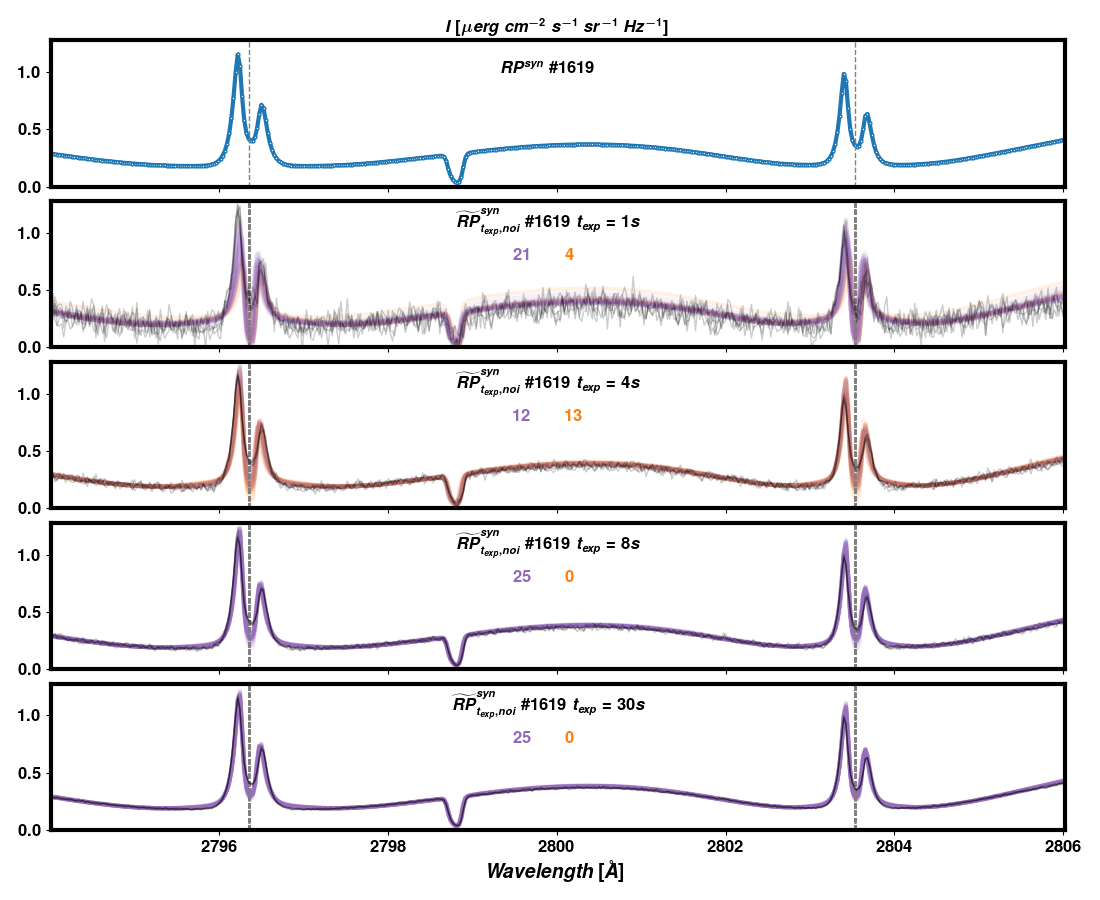
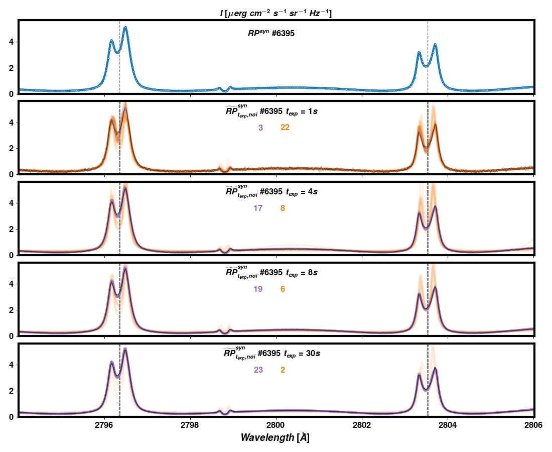
Figure 1: Top panel: The $RP^{syn}$ #1619 is shown in the first row. The four following rows show their corresponding $\widetilde{RP}^{syn}_{t_{exp},noi}$ (in black) for $t_{exp}=1,4,8$ and $30s$, and the "good" and "bad" MC fits in violet and orange respectively (the colored numbers indicate the number of "good" and "bad" MC fits). Bottom panel: the same for $RP^{syn}$ #6395.

2.2 Selection Criteria

The next step is to calculate the uncertainty associated with the $RP^{syn}$-RMA pair. We use the Monte Carlo simulation to calculate the uncertainty for a physical variable as the standard deviation of all the Monte Carlo experiments, that is, the standard deviation of the 25 ${}^{MC}\widetilde{RMA}^{syn}_{t_{exp},noi}$ associated with an $RP^{syn}$. In this context, we refer to a Monte Carlo simulation as the exercise of calculating the 25 inversions for a given $RP^{syn}$(5 times for each of the 5 $\widetilde{RP}^{syn}_{t_{exp},noi}$ associated with that $RP^{syn}$) , and to a Monte Carlo experiment as one of these 25 inversions (or experiments).

In an ideal scenario, we would need a large number of Monte Carlo experiments for each Monte Carlo simulation: this means a large number of independent inversions considering several random initializations of the noise for a given exposure time. In this fashion, the impact of statistical outliers would be reduced compared to our approach with just 25 simulations. However, such an approach is computationally very expensive and not practical. Our current approach to build the "noisy" database required roughly $10M~{}CPU-hours$ executed in the NASA Pleiades supercomputer. A larger number of Monte Carlo experiments or simulations would provide more statistical samples (e.g., $\approx$ 100), but would require many more CPU hours – in the example given $40MCPU-hours$. Such a large number of computational resources is beyond the scope of the current investigation.

As has been mentioned, the standard procedure would be to consider all (25) ${}^{MC}\widetilde{RMA}^{syn}_{t_{exp},noi}$ to calculate the uncertainties (by determining the standard deviation of the physical parameters determined by the inversions in each experiment). However, due to the limited number of simulations, in some cases, only a few fits out of the 25 fits between the $\widetilde{RP}^{syn}_{t_{exp},noi}$ and the resulting inverted profile are "good". In these cases, the standard deviation of these 25 ${}^{MC}\widetilde{RMA}^{syn}_{t_{exp},noi}$ may be very large, since it takes into account a large number of bad fits. Therefore, we adopt a more empirical approach in which the selection of the ${}^{MC}\widetilde{RMA}^{syn}_{t_{exp},noi}$ considered for calculating the uncertainties is based on the goodness of fit between the $\widetilde{RP}^{syn}_{t_{exp},noi}$ and its corresponding inverted profile, i.e., on the value of $\chi^{2}$:

$$\chi^{2}=\frac{1}{\nu}\sum_{i=0}^{q}{(\widetilde{RP}^{syn}_{t_{exp},noi}(\lambda_{i})-I(\lambda_{i};\ ^{MC}\widetilde{RMA}^{syn}_{t_{exp},noi}))^{2}\frac{w_{i}^{2}}{\sigma_{i}^{2}}}$$ (3)

with $\nu$ the number of observables. Note that we are now quantifying the fit between the noisy $\widetilde{RP}^{syn}_{t_{exp},noi}$ and its inverted profile $I$, which is the resulting radiation at $\lambda_{i}$ from the model ${}^{MC}\widetilde{RMA}^{syn}_{t_{exp},noi}$. Thus, for a given $\widetilde{RP}^{syn}_{t_{exp},noi}$, we have 25 values of $\chi^{2}$ corresponding to the fits associated between the $\widetilde{RP}^{syn}_{t_{exp},noi}$ and the 25 inverted profiles $I$ generated by the 25 ${}^{MC}\widetilde{RMA}^{syn}_{t_{exp},noi}$.

We have selected a criterion that considers a large enough number of experiments to preserve some statistical meaning from the Monte Carlo approach, and that also attempts to minimize the impact of bad inversions in the calculation of the uncertainties. To enable this, we always consider at least 10 Monte Carlo experiments. If the number of fits with a $\chi^{2}$ below a given threshold ($\chi^{2}_{threshold}$) is less than 10, then the ${}^{MC}\widetilde{RMA}^{syn}_{t_{exp},noi}$ associated with the 10 best fits are used to calculate the standard deviation of the model. If the number of fits n with $\chi^{2}\leq$ $\chi^{2}_{threshold}$ is larger than 10, then n ${}^{MC}\widetilde{RMA}^{syn}_{t_{exp},noi}$ are used to calculated the uncertainties of the asocciated RMA. To justify this empirical approach, we have analyzed the distribution of the number of inversion fits with a $\chi^{2}$ below different thresholds. Each row of Figure 2 shows the distribution of the number of fits $n$ with a $\chi^{2}$ below a threshold ($\chi^{2}_{threshold}$  indicated in the top left corner in the first column) for each $t_{exp}$ (column) for the case of $0.8\leq\mu<0.9$. The threshold values are $\chi^{2}_{threshold}$$=2,3,3.5$ and $4$. In each individual panel, the percentage of the total number of $n>10$ with with $\chi^{2}\leq$ $\chi^{2}_{threshold}$  is indicated in the top right corner, while in the bottom right corner of the last column is indicated the average of these values for all the $t_{exp}$ at a given $\chi^{2}\leq$ $\chi^{2}_{threshold}$. Figure 3 shows the behavior of the latter average with respect to $\mu$. In this figure, we can see that for $\chi^{2}\leq 3$, except for $\mu=0.55$ and $\mu=0.75$, the averaged-in-$t_{exp}$ percentage of Monte Carlo experiments (inversions) for a given $RP^{syn}$ with at least 10 fits with $\chi^{2}\leq 3$ is larger than 50%, and for the values mentioned before the percentages are very close to 50%. Therefore, we consider $\chi^{2}_{threshold}$$=3$ and $n\geq 10$ to be good criteria to ensure a Monte Carlo simulation with a well-balanced number of good and bad fits at (almost) any $\mu$ and $t_{exp}$ values.

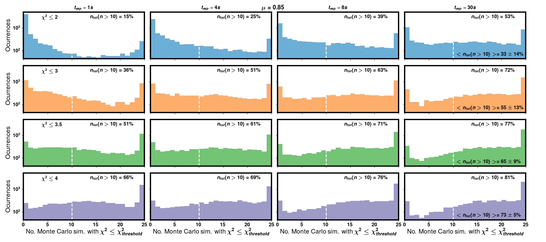
Figure 2: Histograms of number of Monte Carlo simulations (for all $\mathbf{IRIS^{2}}\$ entries with $0.8\leq\mu<0.9$) for which $\chi^{2}\leq$ $\chi^{2}_{threshold}$, with different values of $\chi^{2}_{threshold}$in each row (indicated in upper left of each panel), and different exposure times in each column. Indicated in the top right of each panel is the fraction of cases for which there are at least 10 Monte Carlo simulations with a goodness of fit better than $\chi\leq$ $\chi^{2}_{threshold}$.

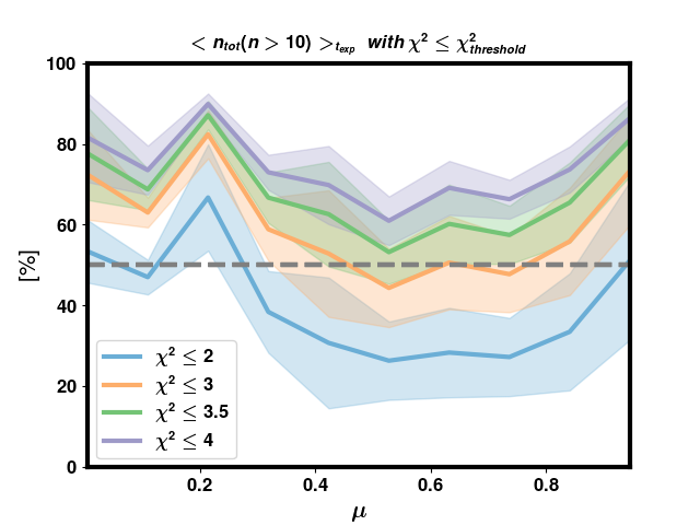
Figure 3: Histogram, as a function of the cosine of the viewing angle ($\mu$), of the average (across all exposure times considered) fraction of $\mathbf{IRIS^{2}}\$ database entries for which there are at least 10 Monte Carlo simulations that meet the goodness of fit criterion $\chi\leq$ $\chi^{2}_{threshold}$. Colors show different values of $\chi^{2}_{threshold}$, while the ranges shown indicate the standard deviation (across different exposure times) on the average fraction.

In summary, the uncertainty of physical variable $p$ in the RMA is calculated as:

$$\sigma_{p}=\sigma(^{[N]}\widetilde{RMA}^{syn}_{t_{exp},noi,p})$$ (4)

with $[N]$ corresponding to the set formed by the $n$ best fits of the Monte Carlo experiments, which are determined by:

$$max(n\ with\ \chi^{2}\leq 3,\ n=10)$$ (5)

For instance, if a $\widetilde{RP}^{syn}_{t_{exp},noi}$ has 16 fits with $\chi^{2}\leq 3$, then $\sigma_{p}$ will be calculated considering their 16 associated ${}^{MC}\widetilde{RMA}^{syn}_{t_{exp},noi}$, i.e. ${}^{[16]}\widetilde{RMA}^{syn}_{t_{exp},noi}$. But, if it has only 3 fits with $\chi^{2}\leq 3$, then $\sigma_{p}$ will be calculated considering the corresponding ${}^{[10]}\widetilde{RMA}^{syn}_{t_{exp},noi}$ to the 10 best fits, including 7 "bad" fits, which will result in a larger uncertainty. We believe this approach captures the impact of the uncertainties introduced by the inversion process. Note that while $MC$ takes values between 1 to 5, $N$ in $[N]$ may take any value from 10 to 25.

3 Discussion

Let us now discuss the impact of these new calculations on the uncertainties on the thermodynamic parameters from $\mathbf{IRIS^{2}}\$, and in particular some cases that highlight the difference between the previous and new approach, and the limitations of any uncertainty calculation.

The first row of Figures 4 and 5 shows the $RP^{syn}$ (first column) and the associated RMAs for $T,v_{los},v_{turb},$ and $n_{e}$ (in the second, thirth, fourth, and fifth column respectively) with the uncertainties calculated using Eq. 3 in Sainz Dalda et al. (2019), i.e., using the response functions. In the following rows, the first column shows $\widetilde{RP}^{syn}_{t_{exp},noi}$ for the $RP^{syn}$#1619 with $t_{exp}=1,4,8,$ and $30s$, with the 5 noise randomizations over-plotted; from the second to the fifth columns the same RMA thermodynamic variables as in the first row, but now showing two types of uncertainties. In blue, we show the uncertainties calculated using the standard deviation of those ${}^{MC}\widetilde{RMA}^{syn}_{t_{exp},noi}$ associated with the inverted profiles for $\widetilde{RP}^{syn}_{t_{exp},noi}$ that satisfy the condition (5). In grey we show the uncertainties derived from all 25 Monte Carlo experiments, i.e., ${}^{[25]}\widetilde{RMA}^{syn}_{t_{exp},noi}$. In each panel of $\widetilde{RP}^{syn}_{t_{exp},noi}$ the number of profiles used to calculate the uncertainty is indicated in black, and, as a reference, the number of profiles that satisfies $\chi^{2}\leq 3$ when that number is less than 10 is indicated in green.

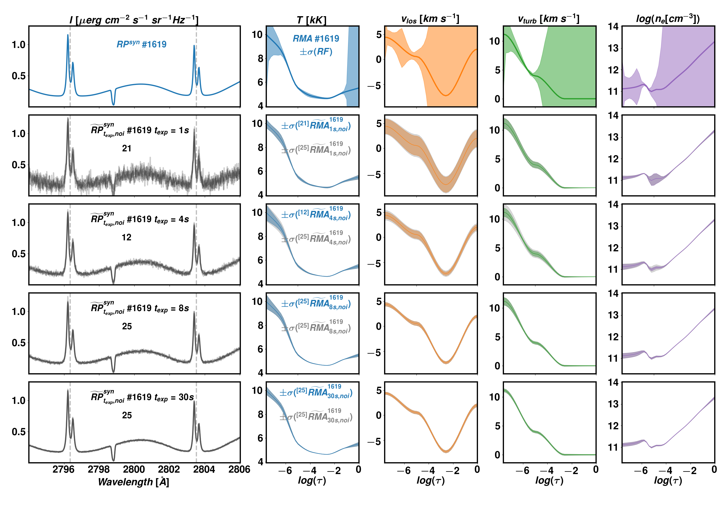
Figure 4: The first column shows the $RP^{syn}$#1619 in blue, and in black its $\widetilde{RP}^{syn}_{t_{exp},noi}$for $t_{exp}=1,4,8,$ and $30s$. The corresponding RMA for $T,v_{los},v_{turb},$ and $n_{e}$ and their uncertainties are shown from the second to the fifth column respectively. In the first row, the uncertainty is obtained from the response functions, while the ones from the second to the fifth rows are obtained by using $N$ Monte Carlo experiments as shown in ${}^{[N]}\widetilde{RMA}^{syn}_{t_{exp},noi}$, for $t_{exp}=1,4,8,$ and $30s$ respectively.

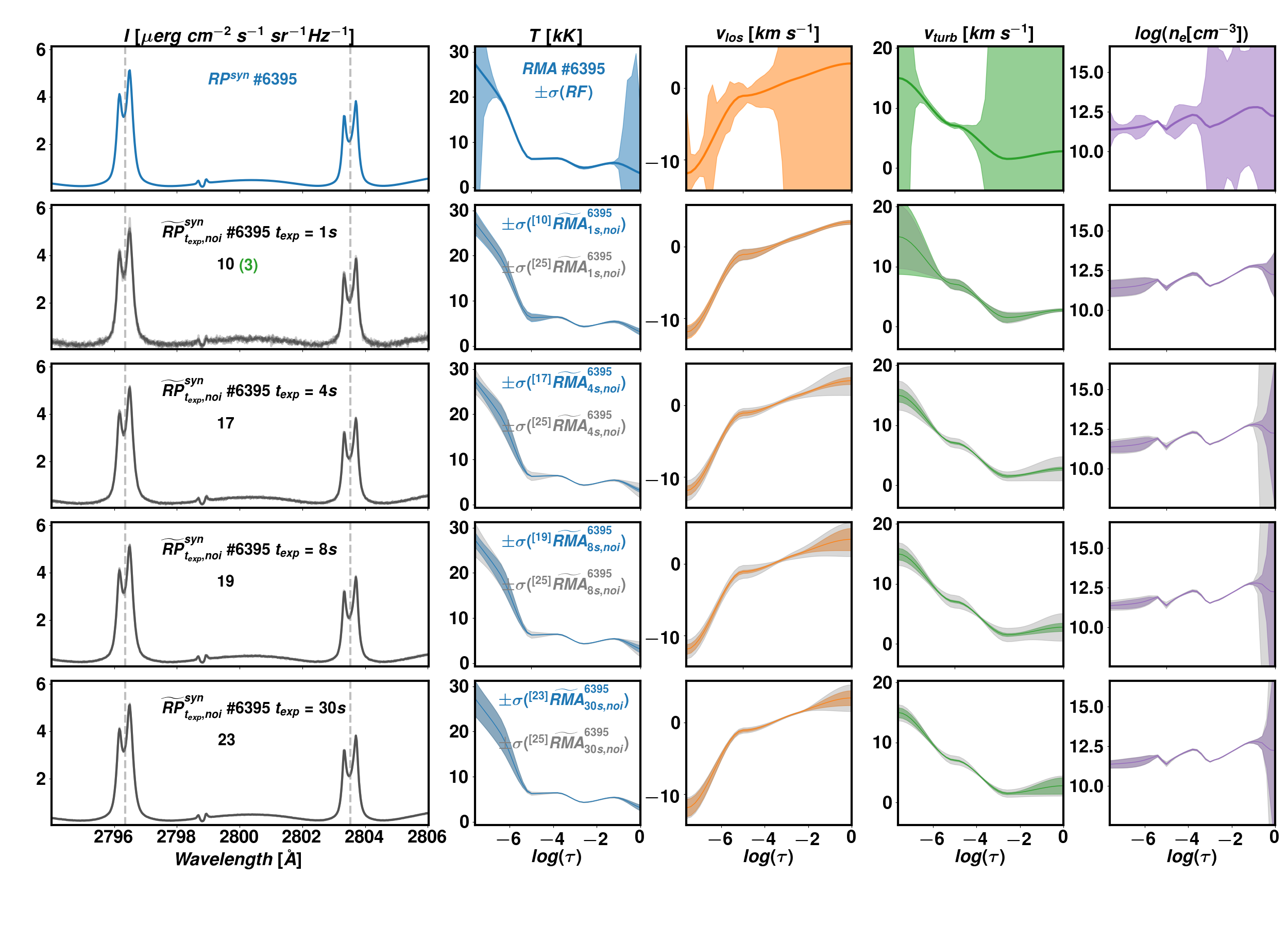
Figure 5: Same as Figure 4 for $RP^{syn}$#6395.

The uncertainties in $T$ are relatively small between $-6\leq log(\tau)\leq-3$ for all the $t_{exp}$ in both examples (#1619 and #6395). When all the 25 Monte Carlo experiments are considered (in grey), we see some differences, with the largest difference at for $-7\leq log(\tau)$ and to a lesser extent around $log(\tau)=-5$. The former location is the region in the optical depth where neither the Mg II h & k nor the Mg II UV2&3 are sensitive to the variations in the thermodynamic variables. The latter is where the Mg II h & k lines are more sensitive to changes in the atmosphere. Therefore, we should expect some uncertainty in the atmosphere for inversion cases in which the $\widetilde{RP}^{syn}_{t_{exp},noi}$ are not well fitted, and also where the Mg II h & k lines are actually sensitive to variations in the thermodynamic parameters. For $-3\leq log(\tau)$, the uncertainties are usually larger, which makes sense since the IRIS Mg II h & k profiles barely encode photospheric information, i.e., these lines are not sensitive to variations in the thermodynamics at this optical depth range.

It is important to distinguish how the uncertainties are calculated in the considered methods. In the method using the RFs, a small variation in the atmospheric parameter is introduced at given optical depth, then the response function is obtained as the difference between the synthetic profile from the atmosphere with the slightly modified parameter with respect to the profile corresponding to the unperturbed model atmosphere (i.e., without variation of any physical parameter). This process is repeated for all the optical depths considered in the model atmosphere. Let us now consider how uncertainties are determined in our new method. First, we note that during the inversion of the profiles only some optical depths (nodes) are considered. In the Monte Carlo approach, five full inversions for the five $\widetilde{RP}^{syn}_{t_{exp},noi}$ are executed to evaluate the reproducibility of the results, using the standard deviation of the resulting models as the uncertainties for the original model. In the first case (using RFs), the synthetic profiles come from a model atmosphere evaluated in all the optical depths with a small variation, while this is not the case in our new calculations: the variation of the model atmosphere during the inversion only occurs in the nodes. In some cases, the inversion code may find a good fit generating some variations in some nodes, and none (or negligible) in other nodes because the code is able to fit the input profile without variation in these nodes. This is why in some cases the uncertainties at $-2\leq log(\tau)$ are very small. This effect can be seen for $v_{los}$ for ${}^{MC}\widetilde{RMA}^{syn}_{t_{exp},noi}$#6395 with $t_{exp}=1s$ in comparison with the other $t_{exp}$. For the latter, the Mg II UV2&3lines are more well defined (less noisy) and the inversion code may be trying to introduce a variation in the nodes at $-3\leq log(\tau)$. This effect is also noted in the $v_{turb}$, and in the $n_{e}$ at $-1\leq log(\tau)$. The conclusion then is that when assessing the uncertainties, we have to be aware of the optical depths where the observed lines are mostly sensitive to different parameters. These regions are slightly different for different solar features (e.g. umbra, penumbra or plage), and different between the physical parameters (e.g., see Fig. 2 in de la Cruz Rodríguez et al. 2016).

The first row of Figure 6 shows maps of the uncertainty calculated using the RFs ($\sigma^{RF}$) of $T,v_{los},v_{turb},$ and $n_{e}$ at $\log(\tau)=-4$. The second and the third rows show respectively the uncertainties calculated using the selective Monte Carlo experiments ($\sigma^{selMC}$) , i.e. ${}^{[N]}\widetilde{RMA}^{syn}_{t_{exp},noi}$, and all 25 Monte Carlo experiments ($\sigma^{all25MC}$), i.e. ${}^{[25]}\widetilde{RMA}^{syn}_{t_{exp},noi}$. At this optical depth, in the plage and the umbra and extended penumbra or canopy the $\sigma^{RF}_{T}<\sigma^{selMC}_{T}<<\sigma^{all25MC}_{T}$, while for the $v_{los}$, $v_{turb}$ , and $n_{e}$ the $\sigma^{RF}>\sigma^{all25MC}>>\sigma^{selMC}$. This situation is however different at $\log(\tau)=-2$ (see Figure 7), where $\sigma^{RF}_{T}>\sigma^{all25MC}_{T}>>\sigma^{selMC}_{T}$, and for the $v_{los}$, $v_{turb}$ , and $n_{e}$ the $\sigma^{RF}>>\sigma^{all25MC}>>\sigma^{selMC}$. These two figures illustrate what we mentioned above. When we calculate uncertainties from the response functions (as in Sainz Dalda et al. 2019), the uncertainties may be too low for those optical depths where the lines are sensitive to changes in the thermodynamics (large RFs), while they may be unrealistically high for those optical depths where the line is barely sensitive to changes in the thermodynamics (small RFs). We find that, for the Monte Carlo approach, the variation with optical depth of the uncertainties is more moderated, and typically smaller for the selective criterion than when considering all 25 Monte Carlo experiments.

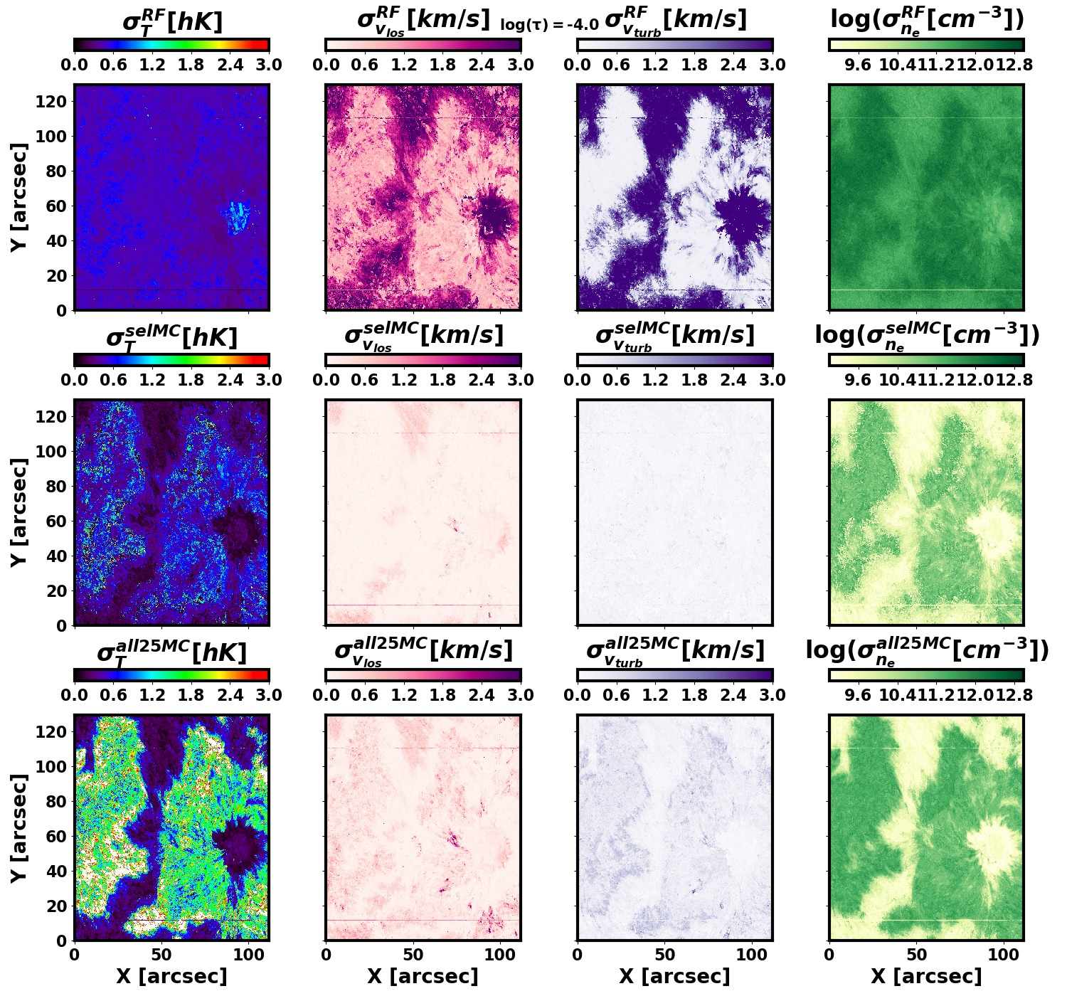
Figure 6: The uncertainties for the $T,v_{los},v_{turb},$ and $n_{e}$ at $\log(\tau)=-4$ when considering the RFs (top row), the selective Monte Carlo approach (middle row), or all the 25 Monte Carlo experiments (bottom row).

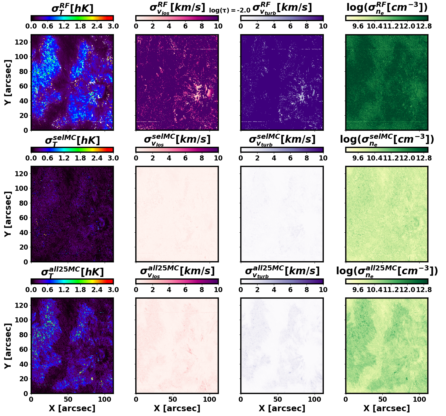
Figure 7: Same as Figure 6 for $\log(\tau)=-2$.

4 Conclusions

In this paper, we present and discuss a novel methodology and the results of applying a selective Monte Carlo approach to determine the uncertainties associated with the Representative Model Atmosphere (RMA) in the $\mathbf{IRIS^{2}}\$ data base. These new uncertainties represent more realistic values than the previously publicly released uncertainties (Sainz Dalda et al., 2019) which were based on response functions. This is because the uncertainties in our new approach have been calculated from the synthetic representative profiles $RP^{syn}$ considering the different sources of uncertainty in the whole process, i.e.: different exposure times, different noise randomization, and different inversion initializations. We define the uncertainty of a physical parameter associated with the pair $RP^{syn}$-RMA as the standard deviation of this parameter in the set of depth-stratified output models (from the Monte Carlo experiments) that satisfy the ad hoc selection criterion shown in Eq. (5). The latter expression is used to minimize the impact of the output models based on inversions that produce a bad fit (with the noisy synthetic profile associated with $RP^{syn}$). In general, at the optical depths where the Mg II h & k and Mg II UV2&3 lines are sensitive to variations in a thermodynamic parameter, the difference between considering all 25 Monte Carlo experiments instead of the number that satisfies expression (5) is very small. The difference is larger for optical depths where the lines are not sensitive to thermodynamic changes.

The new uncertainties will be available to the public in the $\mathbf{IRIS^{2}}\$data base, both for IDL and Python. The uncertainty calculated from the 25 Monte Carlo experiments will also be provided as an extra field in the new version of the $\mathbf{IRIS^{2}}\$data base. Therefore, the new data base will have the following elements:

• $RP^{syn}$: 472 wavelength positions, from 2794 to 2806Å, with a spectral sampling of $\approx 0.025m$Å

• RMA: depth-stratified $T,v_{los},v_{turb},$ and $n_{e}$, sampled at 39 optical depths (i.e., "heights" in the atmosphere) with $\delta log(\tau)=0.2$

• $\sigma_{sel}$: depth-stratified $\sigma_{T},\sigma_{v_{los}},\sigma_{v_{turb}},$ and $\sigma_{n_{e}}$, sampled at 39 optical depths with $\Delta(log(\tau))=0.2$, obtained from the selected Monte Carlo experiments (selective mode). These values are given for $t_{exp}=1,4,8,$ and $30s$. Therefore, $4\times\sigma_{sel}$ values are in the database.

• $\sigma_{all}$: depth-stratified $\sigma_{T},\sigma_{v_{los}},\sigma_{v_{turb}},$ and $\sigma_{n_{e}}$, sampled at 39 optical depths with $\Delta(log(\tau))=0.2$, obtained from the 25 Monte Carlo experiments (all-in mode). These values are given for $t_{exp}=1,4,8,$ and $30s$. Therefore, $4\times\sigma_{all}$ values are in the database.

• $\mu$: from 0 to 1, starting from $\mu=0.05$ at steps of 0.10, as indicated in Table 1.

The different $\mathbf{IRIS^{2}}\$inversion tools that allow users to interface with this database will use these database elements for internal calculations. The inversion of an IRIS Mg II h & k data set will only return the closest $RP^{syn}$ to the observed profiles, the corresponding RMAs, and the uncertainties taking into account the $\mu$ and the $t_{exp}$ of the observation and the uncertainty mode (selective or all-in) chosen by the user.

We believe that the empirical methodology we have developed for $\mathbf{IRIS^{2}}\$will be useful for understanding the uncertainties associated with other or similar inversion approaches.

References

- Bellot Rubio (1998) Bellot Rubio, L. R. 1998, PhD thesis, University of La Laguna, Spain
- Carlsson et al. (2019) Carlsson, M., De Pontieu, B., & Hansteen, V. H. 2019, ARA&A, 57, 189
- Centeno et al. (2021) Centeno, R., de la Cruz Rodríguez, J., & del Pino Alemán, T. 2021, ApJ, 918, 15
- de la Cruz Rodríguez et al. (2016) de la Cruz Rodríguez, J., Leenaarts, J., & Asensio Ramos, A. 2016, ApJ, 830, L30
- de la Cruz Rodríguez et al. (2019) de la Cruz Rodríguez, J., Leenaarts, J., Danilovic, S., & Uitenbroek, H. 2019, A&A, 623, A74
- De Pontieu et al. (2014) De Pontieu, B., Title, A. M., Lemen, J. R., et al. 2014, Sol. Phys., 289, 2733
- De Pontieu et al. (2021) De Pontieu, B., Polito, V., Hansteen, V., et al. 2021, Sol. Phys., 296, 84
- del Toro Iniesta & Ruiz Cobo (2016) del Toro Iniesta, J. C., & Ruiz Cobo, B. 2016, Living Reviews in Solar Physics, 13, 4
- Fontenla et al. (1993) Fontenla, J. M., Avrett, E. H., & Loeser, R. 1993, ApJ, 406, 319
- Ishikawa et al. (2021) Ishikawa, R., Bueno, J. T., del Pino Alemán, T., et al. 2021, Science Advances, 7, eabe8406
- Kerr et al. (2016) Kerr, G. S., Fletcher, L., Russell, A. J. B., & Allred, J. C. 2016, ApJ, 827, 101
- Landi Degl’Innocenti (1979) Landi Degl’Innocenti, E. 1979, Sol. Phys., 63, 237
- Leenaarts et al. (2011) Leenaarts, J., Carlsson, M., Hansteen, V., & Gudiksen, B. V. 2011, A&A, 530, A124
- Leenaarts et al. (2013a) Leenaarts, J., Pereira, T. M. D., Carlsson, M., Uitenbroek, H., & De Pontieu, B. 2013a, ApJ, 772, 89
- Leenaarts et al. (2013b) —. 2013b, ApJ, 772, 90
- MacQueen (1967) MacQueen, J. 1967, in Fifth Berkeley Sympos. Math. Statist. and Probability. I: Statistics, ed. C. University California Press, Berkeley, 281
- Mein (1971) Mein, P. 1971, Sol. Phys., 20, 3
- Pereira et al. (2013) Pereira, T. M. D., Leenaarts, J., De Pontieu, B., Carlsson, M., & Uitenbroek, H. 2013, ApJ, 778, 143
- Quintero Noda et al. (2016) Quintero Noda, C., Shimizu, T., de la Cruz Rodríguez, J., et al. 2016, MNRAS, 459, 3363
- Rubio da Costa et al. (2016) Rubio da Costa, F., Kleint, L., Petrosian, V., Liu, W., & Allred, J. C. 2016, ApJ, 827, 38
- Ruiz Cobo & del Toro Iniesta (1992) Ruiz Cobo, B., & del Toro Iniesta, J. C. 1992, ApJ, 398, 375
- Ruiz Cobo et al. (2022) Ruiz Cobo, B., Quintero Noda, C., Gafeira, R., et al. 2022, A&A, 660, A37
- Sainz Dalda et al. (2019) Sainz Dalda, A., de la Cruz Rodríguez, J., De Pontieu, B., & Gošić, M. 2019, ApJ, 875, L18
- Sánchez Almeida (1997) Sánchez Almeida, J. 1997, ApJ, 491, 993
- Scharmer et al. (2008) Scharmer, G. B., Narayan, G., Hillberg, T., et al. 2008, ApJ, 689, L69
- Steinhaus (1957) Steinhaus, H. 1957, Bull. Acad. Polon. Sci., 4, 801
- Trujillo Bueno & del Pino Alemán (2022) Trujillo Bueno, J., & del Pino Alemán, T. 2022, ARA&A, 60, 415
- Vissers et al. (2022) Vissers, G. J. M., Danilovic, S., Zhu, X., et al. 2022, A&A, 662, A88
- Vissers et al. (2015) Vissers, G. J. M., Rouppe van der Voort, L. H. M., & Carlsson, M. 2015, ApJ, 811, L33
- Westendorp Plaza (1999) Westendorp Plaza, C. 1999, PhD thesis, University of La Laguna, Spain