Benefits of Monotonicity in Safe Exploration with Gaussian Processes
Abstract
We consider the problem of sequentially maximising an unknown function over a set of actions while ensuring that every sampled point has a function value below a given safety threshold. We model the function using kernel-based and Gaussian process methods, while differing from previous works in our assumption that the function is monotonically increasing with respect to a safety variable. This assumption is motivated by various practical applications such as adaptive clinical trial design and robotics. Taking inspiration from the GP-UCB and SafeOpt algorithms, we propose an algorithm, monotone safe UCB (M-SafeUCB) for this task. We show that M-SafeUCB enjoys theoretical guarantees in terms of safety, a suitably-defined regret notion, and approximately finding the entire safe boundary. In addition, we illustrate that the monotonicity assumption yields significant benefits in terms of the guarantees obtained, as well as algorithmic simplicity and efficiency. We support our theoretical findings by performing empirical evaluations on a variety of functions, including a simulated clinical trial experiment.
1 Introduction
The sequential optimisation of an unknown and expensive-to-evaluate function is a fundamental task with a number of interesting challenges. This task arises in various real-world applications, such as robotics [Lizotte et al., 2007], hyperparameter tuning in machine learning [Snoek et al., 2012], environmental monitoring [Srinivas et al., 2012], adaptive clinical trial design [Takahashi and Suzuki, 2021b], recommendation systems [Vanchinathan et al., 2014], and many others. Gaussian process (GP) based techniques such as GP-UCB [Srinivas et al., 2012], Thompson Sampling [Thompson, 1933] and Expected Improvement [Mockus et al., 1978] are particularly popular for this task.
In recent years, a variety of works have considered the important issue of safety, where some actions (function inputs) need to be avoided altogether. Various algorithms such as SafeOpt [Sui et al., 2015], StageOpt [Sui et al., 2018] and SafeOpt-MC [Berkenkamp et al., 2021] have been proposed to tackle this problem. The main idea behind these algorithms is to start with a safe seed set of inputs, and sequentially expand and explore the candidate set of potentially safe points to eventually identify a reachable safe set and/or the maximiser within that set.
In this work, our main goal is to show that monotonicity with respect to just a single input variable can be highly beneficial for this task. Consider a function that we would like to maximise while ensuring that all selected points have value at most .111This is distinct from previous works that require a value of at least , and we discuss the differences in Section 2. We assume that the unknown function is monotonically increasing (not necessarily strictly increasing) with respect to a safety variable , while possibly remaining highly non-monotone with respect to the remaining variables . We consider performance measures based on both a form of cumulative regret and a notion of identifying the entire safe region. Briefly, the benefits of monotonicity in are:
-
(i)
Our theoretical bounds have improved dependencies over previous works, particularly with respect to the domain size (see Appendix C.1 for details).
-
(ii)
By exploiting the monotonicity, we can circumvent the need to explicitly keep track of potential expanders, as existing algorithms do.
-
(iii)
Under monotonicity, continuity, and the mild additional assumption that is always safe, we show that every safe point is reachable, which is not the case for general non-monotone functions.
Intuitively, the presence of the safety variable allows the algorithm to choose how cautious it should be while exploring the domain, and creates a more favourable function landscape for exploration. For instance, the algorithm can “back off” or “proceed with caution” (lower ) when considering less-explored values, but subsequently act more aggressively (higher ) when it becomes more confident that it is safe to do so.
Applications:
Consider the task of adaptive clinical trial design, where the goal is to recruit patients for drug trials in order to evaluate the safety and efficacy of a drug or drug combinations [Coffey and Kairalla, 2008, Berry, 2006]. It is well-accepted that patient characteristics play a significant role in both safety and efficacy given a drug dose [Lee et al., 2020]. Thus, it is helpful to model the drug dose as the safety variable , and patient characteristics as the variable , both of which influence the unknown toxicity, say . For many classes of drugs such as cytotoxic agents, the toxicity and efficacy both increase strictly as the drug dose is increased [Chevret, 2006]. In such cases, for Phase I clinical trials, it is usually necessary to find the Maximum Tolerated Dose (MTD), which is the dose with the maximum toxicity within the permitted threshold for the patient characteristics under consideration [Aziz et al., 2021, Riviere et al., 2014, Shen et al., 2020]. Formulating this task in our problem setting can result in (i) maximisation of benefits (via regret minimisation) and (ii) minimisation of harmful effects to patients involved in the study (via safety constraints), while simultaneously (iii) identifying safety information about the entire set of patient characteristics (via sub-level set estimation), each of which are important goals of adaptive clinical trial design. GP optimisation has been recently used for this task [Takahashi and Suzuki, 2021b, a], but the safety constraints were met in these works by being highly cautious in dose increments (single step increments for discrete dosage levels), and no theoretical guarantees were sought.
Problems in robotics may also serve as potential applications for our problem setup. For example, consider the scenario where a robot performs a task with certain parameters given by the variable , but that there also exists a parameter indicating the speed (or more generally, any measure of “caution” with lower values being more cautious) at which the task is attempted. Then, one may seek to optimise the parameters while ensuring that is never pushed too high to become unsafe, leading to a natural monotonicity constraint. We explore a simple inverted pendulum problem of this kind in Section 5. We note that in some cases, it may be more natural to have separate functions and for measuring reward and safety, and we discuss such variations in Section 3.
Related Work:
Sui et al. [2015] proposed the first algorithm, SafeOpt, for safe GP optimisation. StageOpt was proposed by Sui et al. [2015] as a variation of SafeOpt, where safe set finding and function optimisation were separated into two distinct phases. Berkenkamp et al. [2021] proposed a generalised version of SafeOpt called SafeOpt-MC to tackle the problem when safety functions are decoupled from the function being optimised. Other algorithms such as GOOSE [Turchetta et al., 2019] seek to be more goal-directed during safe set expansion. Safe exploration using Gaussian processes has also been considered by Schreiter et al. [2015], but for the goal of active learning of the unknown function. To our knowledge, none of these works have explored the benefits of having a safety variable leading to monotonicity. Moreover, their theoretical guarantees exhibit certain weaknesses with respect to the domain size that we are able to circumvent; see Section 4 for the details.
Another related line of work introduces algorithms such as GoSafe [Baumann et al., 2021] and GoSafeOpt [Sukhija et al., 2022] to address safe Bayesian optimisation problems. Their setting is fundamentally different to ours, since they consider a dynamic system with time-varying inputs, and allow intervening with a safe backup policy when an imminent safety violation is detected in the original policy. Our setup considers static functions without interventions (which may not be feasible in some applications, e.g., once a drug dose is administered it may not be possible to change).
A different approach to safe GP optimisation is taken in [Amani et al., 2021], in which conditions are explored under which an initial safe seed set can be sampled enough times for the resulting samples alone to expand the safe set significantly (and include the global safe maximiser). However, this requires careful assumptions on the seed set depending strongly on the kernel, and the idea appears to be most suited to finite-dimensional feature spaces (e.g., linear or polynomial kernels); see Appendix C.3 for discussion.
In a parallel line of work, the problem of level set estimation and related settings involving excursion sets has been considered, e.g., see [Gotovos et al., 2013, Bogunovic et al., 2016, Bolin and Lindgren, 2015]. GP optimisation with monotonicity assumptions has also been considered by Li et al. [2017] and Wang and Welch [2018]. However, these works do not consider safety constraints, and consequently, the associated algorithms are significantly different.
A notable prior work combining safety and monotonicity is [Wang et al., 2022], but they study a non-GP setting where all the arms (corresponding to in our setting) are modeled separately, and the goal is best-arm identification. This leads to a precise characterisation of the number of arm pulls. However, their setup, algorithm, and results remain very different from our work, where smoothness with respect to (as well as ) plays a crucial role.
Finally, safety has been considered in a variety of other settings including linear bandits [Amani et al., 2019, Khezeli and Bitar, 2020] and reinforcement learning [Turchetta et al., 2016, Berkenkamp et al., 2017, Turchetta et al., 2020], but compared to the works outlined above for GP settings, these are less directly relevant to ours.
Contributions:
Summarising the above discussions, we list our main contributions as follows:
-
•
We study the problem of safe sequential optimisation of an unknown function, and introduce the idea of considering monotonicity of the function with respect to a “safety” variable. We propose the monotone safe UCB (M-SafeUCB) algorithm for this problem.
-
•
We show that with high probability, M-SafeUCB achieves sub-linear regret (for a suitably-defined regret notion to follow), only selects safe actions, and identifies the safe (sub-level) set of the function with high accuracy.
-
•
We experimentally evaluate M-SafeUCB alongside other baselines on a variety of functions, and demonstrate that the resulting performance aligns with the theoretical guarantees.
2 Problem Statement
We consider the problem of sequentially maximising a fixed but unknown function over a set of decisions while satisfying safety constraints, where , is a compact set and . As discussed above, we assume that the function is monotonically increasing in the first argument. At each round , an algorithm selects an action , and subsequently observes the noisy reward . The action must be chosen at round such that it depends upon the actions picked and the rewards observed up to round , denoted by (i.e., the history). The algorithm is also required to satisfy the safety constraint with high probability.
Goal:
The goals of an algorithm in our problem setting include maximising its cumulative reward and/or finding the entire -sub-level set of , while only choosing safe actions. These desiderata are formalised as follows. For cumulative regret, we consider the following definition:
| (1) |
where we compare against rather than in view of the safety requirement. For the sub-level set, we define
| (2) |
which we seek to approximate to high accuracy (see below). For the safety requirement, we seek that the sampled points satisfy with high probability.
Returning to the notion of the safe sub-level set, we quantify the quality of a solution returned by an algorithm after rounds, with respect to a given point , using the following misclassification loss:
| (3) |
Essentially, this loss function penalises an algorithm heavily for classifying unsafe points as safe, while the penalty for classifying safe points as unsafe increases linearly with the difference in the function value from the threshold. We require that the algorithm should return an -accurate solution with probability at least , i.e.,
| (4) |
We note that the notion of regret that we consider is primarily of interest when coupled with (4), rather than in itself. Small is generally desirable since it implies that we are eventually sampling points with the highest possible safe function value. However, one way of achieving small might be to always choose the same and gradually increasing until a low-regret point is found. The additional condition (4) precludes this possibility.
Assumptions:
Certain smoothness assumptions on the function are necessary in order to be able to provide theoretical guarantees. Similar to much of the earlier work in the area of GP optimisation, we assume that has bounded norm in the reproducing kernel Hilbert space (RKHS) of functions , with positive semi-definite kernel function . This RKHS, denoted by , is completely specified by its kernel function and vice-versa, with an inner product obeying the reproducing property: . The RKHS norm is a measure of the smoothness of with respect to the kernel function , and satisfies if and only if . We assume a known upper bound on the RKHS norm of the unknown target function, i.e., . We also adopt the standard assumption of bounded variance: .
In addition, we make the following assumptions regarding the function domain, monotonicity, and safety:
-
1.
is continuous, while can be either discrete or continuous (our algorithms are written for the discrete case, and we discuss the distinction between the two in Appendix C.2);
-
2.
The function is monotonically increasing in the first argument, i.e., for all , is a non-decreasing function of ;
-
3.
The action is safe for every in the domain, i.e., for all , ;
-
4.
The function exceeds the threshold for at least one point in the domain, i.e., .
The third assumption above is natural since corresponds to the most cautious selection possible, and the fourth assumption is mild since otherwise every action is safe and hence no algorithm would ever choose an unsafe action.
Finally, the noise sequence is assumed to be conditionally -sub-Gaussian for a fixed constant , i.e.,
| (5) |
where is the -algebra generated by the random variables and .
Difference to Existing Settings:
An important distinction between our work and certain previous ones (e.g., [Sui et al., 2015, 2018]) is that we consider all points below the threshold to be safe, rather than all points above the threshold. Our setting corresponds to trying to maximise a function while avoiding the risk of pushing it too far (e.g., dosage in clinical trials), whereas the alternative setting corresponds to needing to avoid excessively low-performance decisions (e.g., parameter configurations that may cause a drone to crash). The resulting algorithms are somewhat different since in our setting, maximisation algorithms will have a natural tendency to move closer to the safety threshold.
While the above difference is important to keep in mind, it is also worth noting that it becomes insignificant when one considers variations of the problem with separate safety and reward functions (see Section 3 for further discussion). In addition, in our experiments we adapt SafeOpt to suit our setting.
3 Proposed Algorithm
Gaussian Process Model:
As is common in prior works, we consider algorithms that use Bayesian modeling (despite the non-Bayesian problem formulation). For this purpose, we use a Gaussian likelihood model for the observations, and a Gaussian process (GP) prior for uncertainty over the unknown function . We let denote a GP with mean and kernel . In the following, we often shorten the GP input to to simplify notation.
The algorithm uses a zero-mean GP, , with being the same as that defining the RKHS. The Gaussian likelihood has an associated variance parameter, which we denote by (i.e., corresponding to additive noise in the Bayesian model).
With the Bayesian model in place, we have the following standard posterior update equations:
| (6) | ||||
| (7) | ||||
| (8) |
Proposed Algorithm:
We propose an algorithm called monotone safe UCB (M-SafeUCB), and provide its theoretical guarantees in Section 4. The key idea is to exploit the knowledge that the function is monotonically increasing in the first argument, , and thus, continually sample points in the domain that have their upper confidence bound equal to the threshold value .
In more detail, M-SafeUCB uses a (standard) combination of the current posterior mean and standard deviation to construct an upper confidence bound (UCB) envelope for the function over , given by
| (9) |
where is a time-dependent constant, that is set as per Lemma 1 below. In each round , it chooses a sample such that (favouring higher in the rare case of having multiple such for a single ). This trades off between exploration and exploitation, i.e., it leads to selection of more points close to the currently optimal solution while exploring as well. If multiple such points are available with UCB equal to , then M-SafeUCB selects the one that has the maximum posterior variance, thus helping to reduce uncertainty and encourage exploration.
To account for all possibilities that may arise in each round , we set the candidate and the candidate set for each as follows:
-
•
If there exists such that , then and ;
-
•
If , , then (based on the assumption that for all , ) and ;
-
•
If , , then .
Next, the set is formed by taking the union over all candidate sets , i.e., . Then, is chosen by maximising the predictive variance:
| (10) |
We note that if no satisfies for a certain , then it must be the case that with high probability, the entire function lies below the safety threshold. This is precluded by assumption 4 of our problem statement. However, with a low probability, it may also be the case that the noisy observations make the function “appear” to be below the threshold to the algorithm. In this low probability scenario, , we set and select as earlier by maximising variance.
While we make the mild assumption that at least one unsafe point exists, if it happens that is safe for all , the algorithm will still eventually identify as safe for every . In this scenario, the problem essentially becomes an unconstrained optimisation problem, and our notion of regret is no longer appropriate (since every point has a strict gap to ).
Finally, at the end of rounds, the algorithm considers the intersection of the confidence regions across all rounds and all , and forms an estimate of the safe sub-level set with respect to the upper bound of this intersection (denoted by ) as follows:
| (11) | ||||
| (12) |
Note on Two-Function Settings:
Throughout the paper, we focus on the case that the function dictates both the objective (higher is better) and the safety (too high is unsafe). However, our ideas can also be applied in scenarios where these functions differ; say, with being the objective and dictating the safety. In the following, suppose that whenever we query a point, we observe noisy samples from both and . The two functions both have RKHS norm at most , and the algorithm can form two separate GP posteriors for them.
First suppose that both and are monotone with respect to . Moreover, similar to the current setup, suppose that the objective is to find the highest possible associated with each . Then, one can simply apply our main algorithm to , with Theorem 2 guaranteeing that we (approximately) find the entire safe boundary. Since both and are monotone, the highest safe for is also the highest safe for , and the overall problem is essentially unchanged compared to the single-function setting. As an example, this scenario corresponds to the task of finding the MTD in clinical trials as discussed in section 1.
In general, one may be interested in scenarios where only is monotone with respect to , whereas is more general. Even in such cases, Algorithm 1 could be used as an initial step to find the safe boundary of , as is guaranteed by Algorithm 1. Then, the safe boundary could be passed to a downstream optimiser that seeks to maximise (either over all safe , or over all for each individual ). This is akin to how the stage-wise algorithm in [Sui et al., 2018] operates.
Finally, more sophisticated algorithms may be possible that utilise information observed about and jointly throughout the course of the algorithm, but such investigations are left for future work.
Note on Contextual Settings:
In some scenarios, it may be useful to incorporate context variable in the problem setup, besides the action variables . For example, a clinical trial setting different from our previous motivating one might consist of choosing a drug dose (with monotone behavior) and the dosage of a different drug (not necessarily monotone), while also having access to patient characteristics (e.g., BMI). All of these impact the drug toxicity, but in contrast to , it may be that cannot be chosen actively and is instead given by “nature”.
In such scenarios, Algorithm 1 can be readily extended to incorporate context variables following the discussion on contextual safe Bayesian optimisation from [Berkenkamp et al., 2021]. This approach allows joint modelling of the unknown function with the variables , so that information can be shared across contexts during optimisation. The proposed selection rule in this case would be: for the given context , search through the ’s and find the highest possible safe associated with each (using the as usual), and then among all candidate ’s, choose to be the one with the highest posterior variance. Since the idea behind this extension closely follows [Berkenkamp et al., 2021], we do not elaborate on it further in this work.
4 Theoretical Results
We present our main theoretical results in this section, under the set of assumptions outlined in 2. The proofs are provided in Appendix A. We note that in asymptotic statements, we treat the dimension and sub-Gaussian parameter (see (5)) as constants, and similarly treat the kernel as fixed.
Lemma 1.
(Theorem 2, [Chowdhury and Gopalan, 2017]) Fix , and suppose that is set as follows:
| (13) |
Then, we have the following with probability at least :
| (14) |
where is the maximum information gain at time :
| (15) |
Here, denotes the mutual information between and , where .
This lemma follows from Theorem 2 from [Chowdhury and Gopalan, 2017]. The quantity is ubiquitous in the GP bandit literature, and quantifies the maximum possible reduction in uncertainty about after observing at a set of points .
Theorem 1.
As an example, with the squared exponential (SE) kernel on a compact subset , is (Srinivas et al., 2010). Thus as , resulting in sub-linear regret. The same holds for the Matérn kernel when the smoothness parameter is not too small.
The following theorem formalises the statement that the algorithm approximately identifies the entire safe region.
Theorem 2.
Substituting the bound on stated above for the squared exponential kernel (or the Matérn kernel when is not too small), we find that as .
The proof of Theorem 1 follows a similar general structure to regret analyses for GP-UCB and related algorithms [Srinivas et al., 2012, Chowdhury and Gopalan, 2017]. In contrast, Theorem 2 requires less standard techniques; see Appendix A for the complete argument.
 |
 |
 |
 |
 |
 |
 |
 |
 |
Dependence on :
As we mentioned in Section 1, our theory circumvents strong dependencies on the domain size that are present in previous works for safe settings, and in fact holds even for continuous domains. The guarantees of SafeOpt [Sui et al., 2015] (and related algorithms in follow-up works) roughly state that the entire reachable safe region, up to deviations of , will be identified with high probability once the time horizon satisfies
| (19) |
where is a suitably-defined constant, and is a safe region that can potentially be reached from some initial safe seed set. While their setup is slightly different from ours (see Section 2), the associated guarantees readily transfer without significant modification. Under the mild assumption that occupies a constant fraction of the domain, the requirement in (19) incurs a linear dependence on the domain size.
Dependence on and :
Our regret bound in Theorem 1 incurs dependence on (up to logarithmic terms), and our convergence rate in Theorem 2 analogously incurs dependence . This dependence matches that of GP-UCB [Srinivas et al., 2012] and other related algorithms for the standard (non-safe) setting, as well as SafeOpt (and others) for the safe setting [Sui et al., 2015].
In the standard setting, it is known that the scaling can be improved to for simple regret [Vakili et al., 2021], and for cumulative regret [Li and Scarlett, 2022, Camilleri et al., 2021]; these improved bounds are near-optimal for common kernels such as Matérn. However, the techniques for attaining this improvement appear to be difficult to apply in the safe setting. For instance, the approaches of [Li and Scarlett, 2022] and [Camilleri et al., 2021] use a small number of batches (e.g., or ). In our setting, the safe set cannot be confidently expanded until the end of each batch, and this may be too infrequent to eventually find the safe boundary. In view of these difficulties, we believe that attaining near-optimal dependence in safe settings would be of significant interest for future work.
5 Experiments
In this section, we present experimental results for M-SafeUCB, and compare the performance to other representative algorithms for safe Bayesian optimisation 222The code is available at https://github.com/arpanlosalka/m-safeucb.. The experiments serve to (i) investigate the cumulative regret of M-SafeUCB and compare against baselines, (ii) compare the boundary of the sub-level set estimated by M-SafeUCB with the actual boundary, and (iii) verify that unsafe points are not sampled during the optimisation. We emphasise that the main goal of this paper is not to have our algorithm outperform or “replace” any baselines. Rather, our main goal is to investigate the benefits of monotonicity, particularly from a theoretical standpoint. We provide the main information regarding the functions, algorithms, and implementation here, and provide more details in Appendix B.
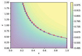
Simulated Clinical Trial:
We first evaluate the performance of M-SafeUCB on a synthetic function that simulates dose-toxicity response of certain drugs. We model toxicity using the logistic function following [Wang et al., 2022], and specifically consider the following:
| (20) |
where and represent the drug dose (safety variable ) and the patient’s age () respectively. As discussed in Section 1, we consider the scenario where both the drug toxicity and efficacy increase monotonically with increasing dosage, and thus, the task reduces to finding the maximum tolerated dose (MTD). We note that while the logistic function is often used to model dose-toxicity response, we incorporate the patient’s age in the function here, such that the toxicity of a drug dose increases as the patient’s age increases. This simulates the scenario that the MTD for a patient with a higher age is lower than that for a patient with a lower age. We set , the toxicity threshold , and the range of inputs is set as (after suitable scale/shift).
We use the Matérn- kernel with trainable length-scale and variance parameters with log-normal priors. Based on minimal manual tuning and seeking simplicity, is set to and is kept constant throughout the optimisation (as in common in the Bayesian optimisation literature).
 |
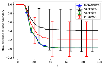 |
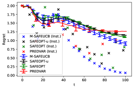
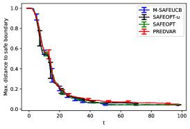
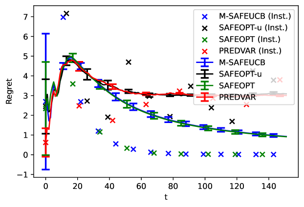
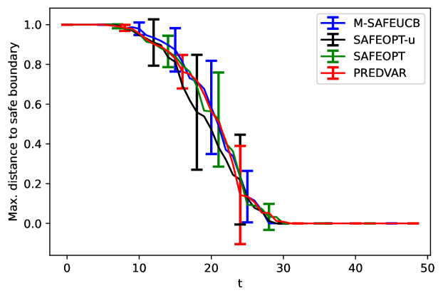
Fig. 1 shows the results obtained by running M-SafeUCB, including the boundary of the safe set estimated, the regret incurred, and the worst-case (over ) distance to the true safe boundary as a function of time. In each case, M-SafeUCB succeeds in estimating the boundary very closely without sampling unsafe points, and the instantaneous regret goes to zero, indicating sub-linear cumulative regret.
We compare the performance of M-SafeUCB with the SafeOpt algorithm [Sui et al., 2015], and an active learning algorithm PredVar, that simply selects the point with the highest posterior variance (among those known to be safe) in each round [Schreiter et al., 2015]. We found that all algorithms maintain the safety requirement, and are roughly equally effective at identifying the safe region. In terms of regret, however, PredVar performs worse, and M-SafeUCB tends to be best.
We note here that we ran the SafeOpt by using the correct estimate of the Lipschitz constant , as well as an underestimate, to demonstrate the effect on performance when a proper estimate of is unavailable (SafeOpt-u in Figure 1). We found that this can result in significantly degraded performance of SafeOpt when is underestimated (see Appendix B for more discussion on the effect of ). Further, SafeOpt incurs a substantially higher computation time due to the requirement of finding the set of potential expanders.
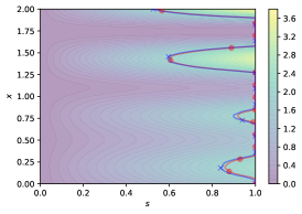
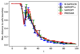
Oscillating Synthetic Functions:
Next, we evaluate the performance of M-SafeUCB on two functions with a more complex form of the safe boundary. The functions are defined as follows:
| (21) | ||||
Both functions are monotonically increasing in the input variable , and satisfy the remaining assumptions, i.e., and , where the input range is set to and the is set to . We use the Matérn- kernel as earlier, and set to for , and 10 for .
Fig. 1 shows the results obtained by running M-SafeUCB, as well as SafeOpt and PredVar. Similar to the earlier results, M-SafeUCB achieves sub-linear regret and finds the entire safe boundary while satisfying safety constraints. SafeOpt also shows similar performance when a good estimate of is available. PredVar and SafeOpt-u perform worse in terms of regret, as can be expected.
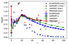
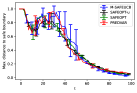
Inverted Pendulum:
We consider the inverted pendulum swing-up problem, a classic control task from the OpenAI Gym [Brockman et al., 2016] as a representative example of problems from robotics that fit into our problem setup. The goal of this task is to apply a torque to the free end of the pendulum to swing it to an upright position, starting from a random initial position. We modify the environment to suit the assumptions of our problem statement (see Appendix B for details). The algorithm is supposed to choose the initial torque that is applied to the pendulum, and the motion is simulated for time steps. We modify the reward function as follows: (i) it equals the original reward if the pendulum does not cross the upright position, (ii) it equals zero if the pendulum reaches the upright position with zero angular velocity, and (iii) if the upright position is crossed, then we let the reward equal the angular velocity at the time of crossing. These changes are made primarily to ensure that the resulting reward function is smooth, and the action of not applying a torque () is safe for all starting positions.
The goal is to maximise the reward function, while ensuring that the upright position is not crossed (thus, ), i.e., case (ii) above is the optimal one, and case (iii) is unsafe.
The experimental results of running M-SafeUCB on this setup are presented in Figure 2, while comparing with SafeOpt and PredVar. We again observe strong similarities in terms of satisfying the safety threshold and finding the safe region. In this case we find that SafeOpt also closely matches M-SafeUCB in terms of regret, albeit at the cost of much higher computation time.
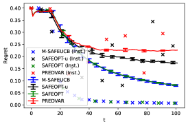
3D Input:
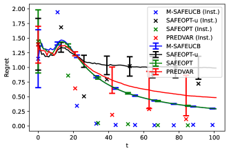
Similar to the earlier experiments involving synthetic functions with 2D inputs, we evaluate the performance of M-SafeUCB on the following function with 3D inputs:
| (22) |
where denotes the safety variable and denotes the other input variable. The domain of each variable is set to , and the safety threshold is set to , thus satisfying the assumptions that for all , and . The average cumulative regret and the instantaneous regret for M-SafeUCB along with other baseline algorithms are shown in Figure 3. We mostly observe similar behavior to the 2D case, except that PredVar now incurs larger error bars.
Summary:
Overall, our experimental results illustrate that (i) explicit expansion is not necessary under our assumed monotonicity conditions, and (ii) monotonicity not only benefits our proposed algorithm, but can also benefit other baselines and safe GP exploration methods in general.
6 Conclusion
We have demonstrated that monotonicity with respect to a single safety variable can have significant benefits for safe GP exploration and optimisation, including improved theoretical guarantees, algorithmic simplicity, and every safe point being reachable under mild conditions. Potential directions for future work include (i) seeking (rather than ) dependence in the theoretical bounds, (ii) further studying more general scenarios with separate functions for safety and reward, (iii) determining other helpful function properties beyond monotonicity, and (iv) studying extensions to reinforcement learning settings, possibly either offline or online.
Acknowledgements.
This work was supported by the Singapore National Research Foundation (NRF) under grant number A-0008064-00-00.References
- Amani et al. [2019] Sanae Amani, Mahnoosh Alizadeh, and Christos Thrampoulidis. Linear stochastic bandits under safety constraints. Advances in Neural Information Processing Systems, 32, 2019.
- Amani et al. [2021] Sanae Amani, Mahnoosh Alizadeh, and Christos Thrampoulidis. Regret bounds for safe Gaussian process bandit optimization. In IEEE International Symposium on Information Theory (ISIT), pages 527–532, 2021.
- Aziz et al. [2021] Maryam Aziz, Emilie Kaufmann, and Marie-Karelle Riviere. On multi-armed bandit designs for dose-finding clinical trials. Journal of Machine Learning Research, 22:1–38, 2021.
- Baumann et al. [2021] Dominik Baumann, Alonso Marco, Matteo Turchetta, and Sebastian Trimpe. Gosafe: Globally optimal safe robot learning. 2021 IEEE International Conference on Robotics and Automation (ICRA), pages 4452–4458, 2021.
- Berkenkamp et al. [2017] Felix Berkenkamp, Matteo Turchetta, Angela Schoellig, and Andreas Krause. Safe model-based reinforcement learning with stability guarantees. Advances in Neural Information Processing Systems, 30, 2017.
- Berkenkamp et al. [2021] Felix Berkenkamp, Andreas Krause, and Angela P Schoellig. Bayesian optimization with safety constraints: Safe and automatic parameter tuning in robotics. Machine Learning, pages 1–35, 2021.
- Berry [2006] Donald A Berry. Bayesian clinical trials. Nature Reviews Drug Discovery, 5(1):27–36, 2006.
- Bogunovic et al. [2016] Ilija Bogunovic, Jonathan Scarlett, Andreas Krause, and Volkan Cevher. Truncated variance reduction: A unified approach to Bayesian optimization and level-set estimation. Advances in Neural Information Processing systems, 29, 2016.
- Bolin and Lindgren [2015] David Bolin and Finn Lindgren. Excursion and contour uncertainty regions for latent gaussian models. Journal of the Royal Statistical Society: Series B: Statistical Methodology, pages 85–106, 2015.
- Brockman et al. [2016] Greg Brockman, Vicki Cheung, Ludwig Pettersson, Jonas Schneider, John Schulman, Jie Tang, and Wojciech Zaremba. OpenAI gym. arXiv preprint arXiv:1606.01540, 2016.
- Bull [2011] Adam D Bull. Convergence rates of efficient global optimization algorithms. Journal of Machine Learning Research, 12(Oct.):2879–2904, 2011.
- Camilleri et al. [2021] Romain Camilleri, Kevin Jamieson, and Julian Katz-Samuels. High-dimensional experimental design and kernel bandits. In International Conference on Machine Learning, pages 1227–1237. PMLR, 2021.
- Chevret [2006] S. Chevret. Statistical Methods for Dose-Finding Experiments. Statistics in Practice. Wiley, 2006.
- Chowdhury and Gopalan [2017] Sayak Ray Chowdhury and Aditya Gopalan. On kernelized multi-armed bandits. In International Conference on Machine Learning, pages 844–853. PMLR, 2017.
- Coffey and Kairalla [2008] Christopher S Coffey and John A Kairalla. Adaptive clinical trials. Drugs in R & D, 9(4):229–242, 2008.
- Gotovos et al. [2013] Alkis Gotovos, Nathalie Casati, Gregory Hitz, and Andreas Krause. Active learning for level set estimation. In International Joint Conference on Artificial Intelligence, pages 1344–1350, 2013.
- Khezeli and Bitar [2020] Kia Khezeli and Eilyan Bitar. Safe linear stochastic bandits. In AAAI Conference on Artificial Intelligence, volume 34, pages 10202–10209, 2020.
- Lee et al. [2020] Hyun-Suk Lee, Cong Shen, James Jordon, and Mihaela Schaar. Contextual constrained learning for dose-finding clinical trials. In International Conference on Artificial Intelligence and Statistics, pages 2645–2654. PMLR, 2020.
- Li et al. [2017] Cheng Li, Santu Rana, Sunil Gupta, Vu Nguyen, and Svetha Venkatesh. Bayesian optimization with monotonicity information. In NeurIPS Workshop on Bayesian Optimization, 2017.
- Li and Scarlett [2022] Zihan Li and Jonathan Scarlett. Gaussian process bandit optimization with few batches. In International Conference on Artificial Intelligence and Statistics, pages 92–107. PMLR, 2022.
- Lizotte et al. [2007] Daniel J Lizotte, Tao Wang, Michael H Bowling, Dale Schuurmans, et al. Automatic gait optimization with Gaussian process regression. In International Joint Conference on Artificial Intelligence, volume 7, pages 944–949, 2007.
- Mockus et al. [1978] Jonas Mockus, Vytautas Tiesis, and Antanas Zilinskas. The application of Bayesian methods for seeking the extremum. Towards Global Optimization, 2(117-129):2, 1978.
- Picheny et al. [2023] Victor Picheny, Joel Berkeley, Henry B. Moss, Hrvoje Stojic, Uri Granta, Sebastian W. Ober, Artem Artemev, Khurram Ghani, Alexander Goodall, Andrei Paleyes, Sattar Vakili, Sergio Pascual-Diaz, Stratis Markou, Jixiang Qing, Nasrulloh R. B. S Loka, and Ivo Couckuyt. Trieste: Efficiently exploring the depths of black-box functions with tensorflow, 2023. URL https://arxiv.org/abs/2302.08436.
- Riviere et al. [2014] Marie-Karelle Riviere, Ying Yuan, Frédéric Dubois, and Sarah Zohar. A Bayesian dose-finding design for drug combination clinical trials based on the logistic model. Pharmaceutical Statistics, 13(4):247–257, 2014.
- Schreiter et al. [2015] Jens Schreiter, Duy Nguyen-Tuong, Mona Eberts, Bastian Bischoff, Heiner Markert, and Marc Toussaint. Safe exploration for active learning with Gaussian processes. In Joint European Conference on Machine Learning and Knowledge Discovery in Databases, pages 133–149. Springer, 2015.
- Shen et al. [2020] Cong Shen, Zhiyang Wang, Sofia Villar, and Mihaela van der Schaar. Learning for dose allocation in adaptive clinical trials with safety constraints. In International Conference on Machine Learning, pages 8730–8740. PMLR, 2020.
- Snoek et al. [2012] Jasper Snoek, Hugo Larochelle, and Ryan P Adams. Practical Bayesian optimization of machine learning algorithms. Advances in Neural Information Processing Systems, 25, 2012.
- Srinivas et al. [2012] Niranjan Srinivas, Andreas Krause, Sham M Kakade, and Matthias W Seeger. Information-theoretic regret bounds for Gaussian process optimization in the bandit setting. IEEE Transactions on Information Theory, 58(5):3250–3265, 2012.
- Sui et al. [2015] Yanan Sui, Alkis Gotovos, Joel Burdick, and Andreas Krause. Safe exploration for optimization with Gaussian processes. In International Conference on Machine Learning, pages 997–1005. PMLR, 2015.
- Sui et al. [2018] Yanan Sui, Vincent Zhuang, Joel Burdick, and Yisong Yue. Stagewise safe Bayesian optimization with Gaussian processes. In International Conference on Machine Learning, pages 4781–4789. PMLR, 2018.
- Sukhija et al. [2022] Bhavya Sukhija, Matteo Turchetta, David Lindner, Andreas Krause, Sebastian Trimpe, and Dominik Baumann. Scalable safe exploration for global optimization of dynamical systems. Artif. Intell., 320:103922, 2022.
- Takahashi and Suzuki [2021a] Ami Takahashi and Taiji Suzuki. Bayesian optimization design for dose-finding based on toxicity and efficacy outcomes in phase I/II clinical trials. Pharmaceutical Statistics, 20(3):422–439, 2021a.
- Takahashi and Suzuki [2021b] Ami Takahashi and Taiji Suzuki. Bayesian optimization for estimating the maximum tolerated dose in Phase I clinical trials. Contemporary Clinical Trials Communications, 21:100753, 2021b.
- Thompson [1933] William R Thompson. On the likelihood that one unknown probability exceeds another in view of the evidence of two samples. Biometrika, 25(3-4):285–294, 1933.
- Turchetta et al. [2016] Matteo Turchetta, Felix Berkenkamp, and Andreas Krause. Safe exploration in finite markov decision processes with gaussian processes. Advances in Neural Information Processing Systems, 29, 2016.
- Turchetta et al. [2019] Matteo Turchetta, Felix Berkenkamp, and Andreas Krause. Safe exploration for interactive machine learning. Advances in Neural Information Processing Systems, 32, 2019.
- Turchetta et al. [2020] Matteo Turchetta, Andrey Kolobov, Shital Shah, Andreas Krause, and Alekh Agarwal. Safe reinforcement learning via curriculum induction. Advances in Neural Information Processing Systems, 33:12151–12162, 2020.
- Vakili et al. [2021] Sattar Vakili, Nacime Bouziani, Sepehr Jalali, Alberto Bernacchia, and Da-shan Shiu. Optimal order simple regret for Gaussian process bandits. Advances in Neural Information Processing Systems, 34:21202–21215, 2021.
- Vanchinathan et al. [2014] Hastagiri P Vanchinathan, Isidor Nikolic, Fabio De Bona, and Andreas Krause. Explore-exploit in top- recommender systems via Gaussian processes. In ACM Conference on Recommender Systems, pages 225–232, 2014.
- Wang and Welch [2018] W. Wang and W. J. Welch. Bayesian optimization using monotonicity information and its application in machine learning hyperparameter tuning. In Proceedings of AutoML 2018 @ ICML/IJCAI-ECAI, 2018.
- Wang et al. [2022] Zhenlin Wang, Andrew J Wagenmaker, and Kevin Jamieson. Best arm identification with safety constraints. In International Conference on Artificial Intelligence and Statistics, pages 9114–9146. PMLR, 2022.
Appendix
Appendix A Proofs
In this section, we present the proofs for Theorem 1 and Theorem 2.
A.1 Proof of Theorem 1 (Regret Bound)
By Lemma 1, with probability at least , the following holds for all and :
| (23) |
where and are the mean and variance of the posterior distribution. As a special case of this fact, at each round , we have
| (24) |
Moreover, given the description of Algorithm 1, we have the following for all :
| (25) |
(Recall that the “safe everywhere” step setting for all will never occur when the confidence bounds are valid, since we assume that at least one point is unsafe.)
Combining the above, we can conclude that for all , with probability at least ,
| (26) |
Hence, we have
| (27) |
Now, from Lemma 4 of [Chowdhury and Gopalan, 2017], . Furthermore, (since is monotonically increasing). Hence, with probability at least ,
| (28) |
A.2 Proof of Theorem 2 (Identification of Safe Boundary)
Again using Lemma 4 in [Chowdhury and Gopalan, 2017], if are the points selected by Algorithm 1, then the sum of predictive standard deviations at these points can be bounded in terms of the maximum information gain as follows:
| (29) |
Using the monotonicity of , we deduce that for , we have
| (30) |
Now, as per Algorithm 1, for all , is one of the following:
-
•
if it holds that ;
-
•
is undefined if it holds that ;
-
•
in all other cases, .
Thus, we can conclude that whenever is defined, it satisfies
| (31) |
This is because is defined based on , whereas considers the minimum of all ’s across to find the maximum .
Since M-SafeUCB selects the point with the largest from the candidate set for , we have the following whenever is defined:
| (32) |
Next, note that is undefined for some only if at round , . In this case, by the definition. Therefore, for all where this occurs for some , we have for all . Hence, as long as the confidence bounds are valid, we have for such .
For all not satisfying the conditions of the previous paragraph, we have for all that there exists such that , and accordingly, is well-defined. In this case, we bound the maximum deviation of from as follows for any :
| (33) | ||||
| (34) | ||||
| (35) | ||||
| (36) |
provided that the confidence bounds are valid. Since this holds for all , we can average both sides over to obtain
| (37) |
where we made use of (A.2). Since , for any , we obtain due to the validity of the confidence bounds. On the other hand, if , there are two sub-cases to consider:
-
•
If and , then
(38) -
•
If and , then
(39) (40) (41)
Therefore, setting , we have the following guarantee for M-SafeUCB’s performance on the sub-level set estimation task:
| (42) |
Substituting into the above choice of completes the proof.
Appendix B Details of Experiments
Gaussian Process Model:
For both the synthetic data and the inverted pendulum experiments, we use a Gaussian Process with Matérn kernel to model the unknown function. We use the Trieste toolbox for implementation [Picheny et al., 2023], and set the length scales and variance of the kernel to be trainable. The initial variance is set by randomly sampling two points in the domain known to be safe, and computing the variance with respect to the observed function values. A log-normal prior is used for both the variance and the length scales, with a standard deviation . The means for the length scales are set to , and that for the variance is . The function values returned are noiseless, while the Gaussian Process regression model assumes a low noise level of for numerical stability. We use the Trieste library for our implementations [Picheny et al., 2023].
Synthetic functions:
The domains of the functions and are set to and . For running the algorithms, the domain is discretised into a grid with linearly spaced points in each dimension. The optimisation is run for iterations for each algorithm. Each experiment is repeated 5 times, and the mean values along with the standard deviations (via error bars) are shown.
For the function , the algorithms are run for iterations, with the domain discretised into a grid with linearly spaced points in each dimension. The experiments are repeated times, and the mean values and standard deviations (via error bars) of the average cumulative regret are shown.
Inverted Pendulum:
For this experiment, we allow the initial angle of the pendulum (denoted by ) to lie in (where angle denotes the upright position), while the applied torque . The angle becomes positive after the pendulum crosses the upright position. We modify the reward function as follows:
| (43) | |||
| (44) |
where and denote the angle and angular velocity of the pendulum at the time step, and denotes the angular velocity of the pendulum when it crosses the upright position, starting with an initial angle and torque of and respectively. Note that the time step (for simulating the motion of the pendulum) is different from the time step (denoting the optimisation iteration).
The safety threshold is set to , which can only happen when both and are (since is always beyond the initial time step) for some . Thus, the safety threshold denotes the condition that the pendulum is in the upright position with a zero angular velocity, resulting in the sustenance of the upright position until the end of the episode, i.e., .
The initial angular velocity is always set to , so that our assumption that is a safe action is satisfied. This is because the pendulum can never swing to the upright position starting from the range of initial positions specified, unless a torque is applied. Furthermore, the initial torque is assumed to be magnified by a factor of when computing the resulting motion, resulting in the possibility of unsafe actions (torque applied, ) corresponding to a large fraction of starting positions (initial angle, ).
Similar to the experiments with synthetic data, the input domain is discretised into linearly spaced points along each dimension, and the results of running the three algorithms 5 times are presented in Figure 2.
Algorithm Details and Discussion:
For SafeOpt, we use the version with the Lipschitz constant as proposed in the original paper [Sui et al., 2015]. We approximate by calculating the gradients for a finely discretised grid of points in the input domain in each case, and take the maximum among their magnitudes. Note that for using SafeOpt in practice, needs to be tuned alongside as a hyperparameter. We consider the “best case” here for SafeOpt, where a close approximation of the original Lipschitz constant for the unknown function is known to the algorithm. For the version of the algorithm using an underestimate of in the experiments, we reduce the estimated by a factor of to . Further, we use the techniques discussed in Section 4 of [Berkenkamp et al., 2017] to reduce the computation cost of SafeOpt. Despite these optimisations, we found that SafeOpt can incur more than ten times the computation cost of M-SafeUCB in our experiments, and this difference increases with increasing input dimension.
As discussed in Section 4 of [Sui et al., 2015], we solely use the confidence intervals for guaranteeing safety, and only use the Lipschitz constant for finding potential expanders. It is important to note here that using the Lipschitz constant for determining the safe set further increases the dependence of SafeOpt on the value of , and can lead to degradation in performance due to over-cautiousness when is overestimated. Thus, we avoid this version of the algorithm in our experiments. We also investigated the modified SafeOpt algorithm suggested in [Berkenkamp et al., 2017] that avoids the dependence on altogether, but we found it to be substantially more time consuming to run.
We also note here that in the version of SafeOpt used in our experiments as described above, overestimating essentially makes the algorithm behave very similar to M-SafeUCB, since the number of points included in the set of potential expanders is small (or even zero) due to over-cautiousness, while the set of maximisers remains unaffected since is determined only using the confidence intervals of the GP. This leads to wasteful computation compared to M-SafeUCB leading to a greatly increased running time for obtaining a similar performance, thus also showcasing the benefits of using M-SafeUCB over SafeOpt for the problem setup under consideration.
For the PredVar algorithm, we consider the variance of all points in the domain with (since these are known to be safe), as well as the points that can be guaranteed to be safe based on at time step , and choose the one with the highest variance.
We also note that M-SafeUCB is similar in spirit to the (SafeUCB) baseline [Sui et al., 2015], which simply maximises the UCB among all points that are known (with high probability) to be safe. However, doing this naively would lead to focusing on a small region of the space and ignoring the rest. M-SafeUCB overcomes this by using the maximum-variance rule.
Appendix C Further Discussion
C.1 Discussion on Dependence
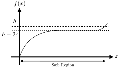
To get some intuition on why a linear dependence on the domain size may arise for algorithms such as SafeOpt (as discussed in Section 4), consider the function shown in Figure 4. Once the function reaches , it may become very difficult to use the confidence bounds and Lipschitz constants (as SafeOpt uses) to determine whether it is still safe to move further to the right. One can imagine that an algorithm ends up sampling every (or at least most ) even if is discretised rather finely, particularly if the Lipschitz constant is over-estimated.
On the other hand, we highlight some potential weaknesses of SafeOpt via two perspectives as follows:
-
(i)
If the domain is quantised very finely, then one should only expect a number of samples depending on , rather than . This is because once a given point with has its function value known accurately (say, to within ), one should be able to certify the entire surrounding region of width as safe, rather than only the next point to the right.
-
(ii)
One can attain a guarantee with having or even dependence (up to logarithmic factors) using a fairly trivial algorithm: Repeatedly sample all (known) safe points until their function values are known to within using basic concentration bounds, then expand the safe set using the Lipschitz constant, then return to repeated sampling (only for points not yet sampled), and so on. (Logarithmic terms would then arise from applying the union bound.) The resulting guarantee would even further improve SafeOpt’s guarantee due to omitting on the left-hand side.
Despite these limitations, we note that SafeOpt has been an important and highly influential algorithm since its introduction, and the above discussion is only meant to highlight that its theoretical guarantees, while valuable, may leave significant room for improvement in certain scenarios.
C.2 Computational Considerations
As stated, Algorithm 1 involves an explicit loop over all . This is feasible when the domain size is small, and we adopted it in our experiments. However, such an approach may become infeasible for large or continuous domains. In such cases, one may need to rely on approximations or alternative methods, some of which we briefly discuss here.
First, if the domain is continuous, then one could rely on any constrained black-box (non-convex) optimisation solver to minimise the posterior variance subject to the UCB being at most . For commonly-used kernels, the posterior variance and UCB are differentiable, which can facilitate this procedure. Moreover, to handle the possibility of points with being selected, a second constrained black-box search could be performed over all subject to the UCB being at least . The final selected point would then be the higher-variance one among the two points identified.
If no suitable black-box solver is available, or if the domain is discrete but large, then a simple practical alternative is as follows. Instead of performing a full optimisation of the acquisition function, one can randomly select a moderate number of points at random (e.g., 500 or 1000) and only optimise over those. Due to the randomness, ’s throughout the entire domain will then be considered regularly with high probability. Moreover, the efficiency could potentially be improved by ruling out certain regions early (e.g., when is known to be safe). Note, however, that we do not claim any theoretical guarantees under these variations of the algorithm.
C.3 Discussion of Amani et al. [2021]
As we discussed in Section 1, the approach of [Amani et al., 2021] is based on first expanding the safe set using sufficiently many samples within an initial seed set. To highlight a limitation of this approach for certain kernels with infinite-dimensional feature spaces, consider the Matérn kernel, and suppose that the initial seed set includes a large fraction of the domain, but the function value is zero within that entire set. Since compactly supported “bump” functions are in the Matérn class [Bull, 2011], the function may contain both positive and negative bumps outside the seed set, some of which are safe and some of which are not. (Here we only assume that is safe.) Since the function is zero within the seed set, there is no way that its samples can distinguish between these two cases.
In contrast, for finite-dimensional feature spaces (e.g., the linear or polynomial kernel) even samples within a small seed set can indeed be sufficient to accurately learn the entire function. Finally, for the infinite-dimensional case with very rapidly decaying eigenvalues (e.g., SE kernel), the situation is somewhere in between the preceding examples; in particular, compactly supported functions are not in the RKHS. In such scenarios, the approach of [Amani et al., 2021] may be feasible, though the precise details become somewhat complicated; certain results for infinite-dimensional settings are given in [Amani et al., 2021] accordingly.