Embed and Emulate: Learning to estimate parameters of dynamical systems with uncertainty quantification

Abstract

This paper explores learning emulators for parameter estimation with uncertainty estimation of high-dimensional dynamical systems. We assume access to a computationally complex simulator that inputs a candidate parameter and outputs a corresponding multichannel time series. Our task is to accurately estimate a range of likely values of the underlying parameters. Standard iterative approaches necessitate running the simulator many times, which is computationally prohibitive. This paper describes a novel framework for learning feature embeddings of observed dynamics jointly with an emulator that can replace high-cost simulators for parameter estimation. Leveraging a contrastive learning approach, our method exploits intrinsic data properties within and across parameter and trajectory domains. On a coupled 396-dimensional multiscale Lorenz 96 system, our method significantly outperforms a typical parameter estimation method based on predefined metrics and a classical numerical simulator, and with only 1.19% of the baseline’s computation time. Ablation studies highlight the potential of explicitly designing learned emulators for parameter estimation by leveraging contrastive learning.

1 Introduction

Physics-based simulators play a vital role in many domains of science and engineering, from energy infrastructure to atmospheric sciences. They are frequently critical for assessing risk and exploring “what if” scenarios, which require running models many times (Snyder et al., 2019; Beusch et al., 2020; Helgeson et al., 2021; Zhao et al., 2021). However, the increasing complexity of operational computer models makes running such simulators a major challenge. Emulators (also known as surrogate models) are models trained to mimic numerical simulations at a much lower computational cost, particularly for parameters or inputs that have not been simulated.

This paper considers the problem of estimating the parameters of a physics simulation that provide the best fit to data. The estimation problem can generally be thought of as a nonlinear inverse problem in which our goal is to estimate parameters ${\boldsymbol{\phi}}\in\mathbb{R}^{k}$ from a noisy multichannel time series $\mathbf{Z}\in\mathbb{R}^{T\times d}$. $\mathbf{Z}=H({\boldsymbol{\phi}};\mathbf{Z}_{0})+\boldsymbol{\eta}$, where $H({\boldsymbol{\phi}};\mathbf{Z}_{0})$ represents running is a physics simulator with parameters ${\boldsymbol{\phi}}$ and initial condition $\mathbf{Z}_{0}$ for $T$ time steps, and $\boldsymbol{\eta}\sim\mathcal{N}(0,\boldsymbol{\Gamma})$ is observation noise. To ease the notation, we drop the initial condition $\mathbf{Z}_{0}$ in $H({\boldsymbol{\phi}};\mathbf{Z}_{0})$. We are particularly interested in complex simulators for which we do not have analytic expressions for $H$, evaluating $H({\boldsymbol{\phi}})$ is a computational bottleneck and we cannot readily compute its gradients.

One important application of this problem arises in climate science, where climate scientists have spent decades developing sophisticated physics-based models corresponding to $H$, often implemented using large-scale software systems that solve complex systems of differential equations (Kay et al., 2015). In this case, evaluating $H$ can be computationally demanding. Furthermore, tools like physics-informed neural networks (Raissi et al., 2019) are inapplicable because we cannot compute losses that depend upon knowing the form of $H$. Estimating the parameters of such models based on observational data is essential for accurate climate forecasting, and we typically seek not only point estimates of parameters, but also quantifiable uncertainty measures that allow us to forecast the full range of possible future outcomes. Parameter uncertainty quantification is vital here (Cleary et al., 2021; Souza et al., 2020; Hansen, 2022), especially when dealing with noisy observations where a small error in $\hat{\boldsymbol{\phi}}$ might lead to a dramatically different forecasts of the dynamics; uncertainty quantification also plays a vital role in the decision-making process to prevent hazardous loss under tail events (Hansen, 2022).

We explore an alternative framework in which we use our simulator to generate training samples of the form $({\boldsymbol{\phi}}_{i},\mathbf{Z}_{i})$ for $i=1,\ldots,n$ and train a machine learning model for parameter estimation. Our approach, which we call Embed & Emulate, jointly trains two neural networks. The first, $f_{\theta}$, maps an observation $\mathbf{Z}$ to a low-dimensional embedding. The second, $\hat{g}_{\theta}$, emulates the map $g_{\theta}:=f_{\theta}\circ H$, and so maps a parameter vector ${\boldsymbol{\phi}}$ to the same low-dimensional embedding space. The learned $\hat{g}_{\theta}$ may be used in place of $H$ within an optimization-based framework such as Ensemble Kalman Inversion (EnKI, Section 2).

More specifically, our method uses the learned low-dimensional embedding to specify an objective function well-suited to parameter estimation without expert knowledge and the learned emulator as a surrogate for classical numerical methods used to compute $H$. Furthermore, inspired by empirical Bayes methods, our learned network suggests a natural mechanism for specifying the EnKI prior based on the trained network.

2 Related work

Brief parameter estimation background

A widely-used approach for parameter estimation is Ensemble Kalman Inversion (EnKI; Section A.1) (Iglesias et al., 2013). EnKI is a derivative-free optimization framework allows a user to specify a prior distribution over the parameter vector ${\boldsymbol{\phi}}$ and results in samples from the corresponding posterior distribution. As a result, this method provides users with important information about the uncertainty of estimates of ${\boldsymbol{\phi}}$. The clear and thought-provoking paper of Schneider et al. (2017) highlighted the use of the EnKI in earth system modeling.

Despite its success in the perfect-model setting (i.e., where $H({\boldsymbol{\phi}})$ can be computed exactly and perfectly represents the dynamics in $\mathbf{Z}$ for some ${\boldsymbol{\phi}}$), using such methods in practice presents several challenges. To use the EnKI for parameter estimation, we must specify three key elements: (a) the objective function that EnKI is attempting to minimize; (b) the tool used to compute the forward mapping $H$ (or a surrogate for $H$); and (c) a prior $p_{\boldsymbol{\phi}}$. For instance, Schneider et al. (2017) uses a Gaussian prior $p_{\boldsymbol{\phi}}$, computes $H$ using Runge-Kutta methods (Dormand and Prince, 1980), and attempts to minimize the Mahalanobis distance

$$J_{\rm moment}({\boldsymbol{\phi}}):=\|m(\mathbf{Z}_{i})-m(H({\boldsymbol{\phi}}))\|_{\boldsymbol{\Sigma}(m(\mathbf{Z}_{i}))}^{2},$$ (1)

where $m(\mathbf{Z}_{i})$ is a vector of first and second moments of different spatial channels of $\mathbf{Z}_{i}$ and $\boldsymbol{\Sigma}_{i}$ is a diagonal matrix with the $j$-th diagonal entry $\boldsymbol{\Sigma}_{i,j,j}:={\rm Var}[m(H({\boldsymbol{\phi}}_{i}))_{j}]$. Using a loss based on moments within the EnKI framework provides critical robustness to the chaotic nature of $\mathbf{Z}_{i}$.

This framework presents two central challenges. First, choosing the objective for EnKI to minimize requires non-trivial domain knowledge, and a poor choice may lead to biased parameter estimates or unpredictable sensitivities to certain features in $\mathbf{Z}$. Second, high-resolution simulations used to evaluate $H$ for a given ${\boldsymbol{\phi}}$ (e.g. Runge-Kutta or other classical numerical solvers) can be computationally demanding. In particular, the EnKI method uses a collection of particles to represent samples of the posterior, and the forward model $H$ must be calculated for each particle at each iteration. For complex optimization landscapes or in high-dimensional settings, the number of particles must be large. This is further complicated by the fact that often the parameter estimation task is conducted repeatedly, e.g., each time new climate data is acquired.

Simulation-based inference (SBI): A large body of work in SBI focuses on parameter estimation for physics-based simulators (Beaumont et al., 2009; Papamakarios et al., 2019; Cranmer et al., 2020; Lueckmann et al., 2019; Chen et al., 2020b; Alsing et al., 2019). Advanced SBI methods focus on adaptive generation of new training data to approximate the posterior and could be classified into different categories based on how they adaptively choose informative simulations (Lueckmann et al., 2021). One approach, likelihood estimation, proposes to approximate an intractable likelihood function (Drovandi et al., 2018). For instance, Sequential Neural Likelihood estimation (SNL, Papamakarios et al. (2019)) trains a conditional neural density estimator (e.g., Masked Autoregressive Flow (MAF)) which models the conditional distribution of data given parameters (Papamakarios et al., 2017)). While SNL does not readily scale to high-dimensional data, a recent variant called SNL+ (Chen et al., 2020b) addresses this limitation by learning sufficient statistics (embeddings) of the data based on the infomax principle, and it iteratively updates the network used to compute sufficient statistics and the neural density estimators during sequential sampling. An alternative approach, (sequential) neural posterior estimation ((S)NPE), aims to approximate directly the target posterior (SNPE-A in Papamakarios and Murray (2016), SNPE-B in Lueckmann et al. (2017), SNPE-C in Greenberg et al. (2019)), where SNPE-C forces fewer restrictions on the form of prior and posterior by leveraging neural conditional density estimation.

However, in the context of this manuscript’s setting, i.e., estimating multiple $\boldsymbol{\phi}_{i}$ for multiple different observations $\mathbf{Z}_{i}$ at test time, the key technique of SBI, sequential sampling, can require substantial computational investments. This idea is discussed further with our experimental results.

Learned emulators

Physics models and simulations are pervasive in weather and climate science, astrophysics, high-energy and accelerator physics, and the study of dynamical systems. These models and simulations are used, for example, to infer the underlying physical processes and equations that govern our observations, design new sensors or facilities, estimate errors, understand experimental behavior, and estimate unknown parameters within models. Many such physics simulators require expensive computational resources, and are difficult to fully leverage. “Learned emulators,” “surrogate models,” or “approximants” are computationally-efficient approximate models that use numerically simulated data to train a machine learning system to mimic these numerical simulations at a much smaller computational cost. There have been many recent successes in the development of surrogate model foundations (Brockherde et al., 2017; Raissi et al., 2019; Chattopadhyay et al., 2019, 2020; Raissi et al., 2017; Vlachas et al., 2018, 2020; Brajard et al., 2020; Gagne et al., 2020) and applications (Goel et al., 2008; Mengistu and Ghaly, 2008; Brigham and Aquino, 2007; Kim et al., 2015; Papadopoulos et al., 2018; White et al., 2019; Gentine et al., 2018; Rasp et al., 2018; Cohen et al., 2020; Yuval and O’Gorman, 2020; Xue et al., 2021; Wang et al., 2019).

Typically, one would directly try to emulate $H$, and the efficacy of the learned emulator would be evaluated on how well $\hat{H}({\boldsymbol{\phi}})$ matches $H({\boldsymbol{\phi}})$ (often using squared error) across a range of ${\boldsymbol{\phi}}$. This formulation, however, may be suboptimal when the emulator will be used for parameter estimation. First, as we will detail later, emulating $H$ when $\mathbf{Z}$ is very high-dimensional is quite challenging. (In our experiments, ${\rm dim}(\mathbf{Z})=396,000$.) Furthermore, in many climate settings, $H$ represents a chaotic process in which very small changes to the initial conditions can result in very large differences later in the process. In this setting, training an emulator with a loss akin to $(1/n)\sum_{i=1}^{n}\|\mathbf{Z}_{i}-\hat{H}({\boldsymbol{\phi}}_{i})\|_{2}^{2}$ may be overly sensitive to noise and initial conditions and not preserve statistical features of $\mathbf{Z}_{i}$ that may be essential to parameter estimation.

Inspired by the objective in (1), Cleary et al. (2021) trained a model $\hat{g}_{\theta}$ to emulate the moments of parameters using the loss function $\ell_{\rm moment}(\theta):=(1/n)\sum_{i=1}^{n}\|m(\mathbf{Z}_{i})-\hat{g}_{\theta}({\boldsymbol{\phi}}_{i}))\|_{\boldsymbol{\Sigma}_{i}}^{2}$ to ease the burden of running $H$. However, $\ell_{\rm moment}(\theta)$ is not always the best choice. First, estimating $\boldsymbol{\Sigma}_{i}$ for each training sample is an enormous computational burden that far exceeds the cost of generating the original training data (unless the range of candidate ${\boldsymbol{\phi}}$ is very small). Second, choosing the moment function $m$ (essentially fixing a particular low-dimensional embedding) is a critical design element that requires domain expertise and often must be tuned in practice. Finally, even if one is willing to generate accurate estimates of $\boldsymbol{\Sigma}_{i}$, one could face additional challenges. Cleary et al. (2021) is designed for inferring parameters given one fixed test observation, and they train their emulator for a small domain of parameter space dependent on the test observation at hand. Extending this framework to a larger domain of parameters ${\boldsymbol{\phi}}$ results in large variability among the collection of corresponding $\boldsymbol{\Sigma}_{i}$s generated for training, making the loss landscape challenging to navigate.

Contrastive learning

With the above challenges in mind, we present a novel and generic framework for parameter estimation by jointly optimizing (a) an embedding of the multichannel dynamics used to evaluate the accuracy of a candidate parameter ${\boldsymbol{\phi}}$ and (b) an emulator of the dynamics projected into the embedding space. We leverage a contrastive framework to learn discriminative representations for high-dimensional spatio-temporal data.

Contrastive representation learning has exploded in popularity recently for self-supervised visual feature learning that has achieved comparable performance with its supervised counterparts (Caron et al., 2020; Chen et al., 2020a; He et al., 2020; Grill et al., 2020; Zhang and Maire, 2020; Caron et al., 2021). The majority of these frameworks operate under the push-pull principle for instance-wise discrimination: images generated from different forms of data augmentation (e.g., cropping, color jittering) are pulled together while other images are pushed away. Apart from its common setup in unsupervised representation learning, Khosla et al. (2020) also demonstrated selecting positive and negative pairs in a supervised way leveraging label information can boost the performance. Many efforts focus on understanding the mechanism of contrastive learning (Oord et al., 2018; Wei et al., 2020; Arora et al., 2019; Wang and Isola, 2020; Zimmermann et al., 2021). Among them, Zimmermann et al. (2021) show that contrastive loss can be interpreted as the cross-entropy between the latent conditional distribution and ground truth distribution.

3 Contributions

In our work, we follow the contrastive framework and learn an embedding network to capture structural information for high-dimensional spatio-temporal data and an emulator that can be used to compute parameter estimates with uncertainty estimates. This is effective for several reasons. First, when the model $H$ is bijective, representations learned using contrastive losses are highly correlated with their underlying parameters (Zimmermann et al., 2021). Second, most existing emulating methods focus on approximating dynamical models for a fixed parameter ${\boldsymbol{\phi}}$ and lack generalization capacity (Krishnapriyan et al., 2021). In part this is due to the difficulties of emulating dynamics with high spatio-temporal resolution. We circumvent this bottleneck by training an emulator to output the learned latent representations of the dynamics, which are much lower-dimensional and easier to learn with fewer training samples. Finally, our method is inspired by the Contrastive Language–Image Pre-training (CLIP) (Radford et al., 2021) framework, which is designed for contrastive learning of aligned representations of images and language. Our approach, by analogy, learns aligned representations of dynamics and parameters, allowing us to jointly learn the embedding function and emulator for high-resolution data.

More specifically, this paper makes the following key contributions:

• Incorporation of a contrastive loss function for learning an embedding of the simulation outputs ($\mathbf{Z}_{i}$) instead of relying on a known “good” moment function $m$, leveraging ideas from CLIP (Radford et al., 2021);

• Development of an emulator designed to facilitate parameter estimation with uncertainty quantification. We demonstrate that the proposed emulator can be used effectively within an EnKI framework to generate parameter estimates with accurate posterior distribution estimates.

• An empirical evaluation of different methods (EnKI (Schneider et al., 2017), supervised learning, NPE-C Greenberg et al. (2019), SNL+ (Chen et al., 2020b), and our proposed emulator-based approach) in terms of robustness to noise or errors in training and testing data for a range of sample sizes as well as computational costs. Compared to using numerical solvers, we show that our method achieves higher accuracy overall in 1.08% of the computation time, even accounting for the computational costs of generating training data.

• Evaluation of the quality of the uncertainty estimates using the Continuous Ranked Probability Score (CRPS) for varying numbers of training samples.

Our empirical results highlight both the improved computational and empirical accuracy of our proposed emulator-centric approach relative to competing methods and, more broadly, the benefits of designing emulators specifically for parameter estimation tasks.

4 Proposed method

Our goal is to learn a mapping from observations of a multichannel dynamical system, $\mathbf{Z}\in\mathbb{R}^{T\times d}$, to the underlying system parameters ${\boldsymbol{\phi}}\in\mathbb{R}^{k}$, where $\mathbf{Z}=H({\boldsymbol{\phi}})+\boldsymbol{\eta}$ for some noise vector $\boldsymbol{\eta}\in\mathbb{R}^{T\times d}$. We assume we do not have access to an analytical expression for $H$, but can compute $H({\boldsymbol{\phi}})$ for any ${\boldsymbol{\phi}}$ using a computationally complex simulator. We further assume a prior $p_{\boldsymbol{\phi}}$ over parameter space.

Using this prior and the simulator, we generate $n$ training samples as follows: for $i=1,\ldots,n$, draw ${\boldsymbol{\phi}}_{i}\sim p_{\boldsymbol{\phi}}$, and use the simulator to compute $\mathbf{Z}_{i}=H({\boldsymbol{\phi}}_{i})+\boldsymbol{\eta}_{i}$. We do not explicitly generate noise $\boldsymbol{\eta}_{i}$; rather, the numerical algorithm used to simulate $H$ will generally produce some errors, with faster implementations of $H$ being more error-prone. The distribution $p_{\boldsymbol{\phi}}$ coupled with the noise distribution over $\boldsymbol{\eta}$ induces the joint distribution $p_{{\boldsymbol{\phi}},\mathbf{Z}}$.

4.1 Baseline approach – supervised learning

Given training samples $({\boldsymbol{\phi}}_{i},\mathbf{Z}_{i})$ for $i=1,\ldots,n$, we train a neural network represented by $h_{\theta}$ using a ResNet (He et al., 2016) as the backbone (see details in Section B.2). $\theta$ denotes the learned network parameters and our prediction is $\hat{\boldsymbol{\phi}}_{i}=h_{\theta}(\mathbf{Z}_{i})$. We train using the Mean Absolute Percentage Error (MAPE) loss

$$\ell_{\rm MAPE}(\theta):=\frac{1}{n}\sum_{i=1}^{n}\sum_{j=1}^{k}\left|\frac{{\boldsymbol{\phi}}_{ij}-(h_{\theta}(\mathbf{Z}_{i}))_{j}}{|{\boldsymbol{\phi}}_{ij}|+\epsilon}\right|.$$ (2)

As we will see in the experimental results, this approach yields point estimates of ${\boldsymbol{\phi}}$ on holdout test data with reasonable accuracy and offers a significant computational advantage over the EnKI method. However, it does not offer uncertainty estimates, and its test accuracy is lower than that of our proposed approach (Section 4.2).

4.2 Our approach: joint embedding and emulation via contrastive feature representation

Contrastive feature representation: Measuring the distance between a pair of dynamics, a necessary task for constructing a loss function used for training, is particularly challenging when the dynamics are chaotic. As mentioned above (Section 2), one alternative in the literature is to use a custom loss function based on summary statistics of $\mathbf{Z}$; this requires expert knowledge to determine which statistics are relevant, and has demonstrated efficacy only for narrow ranges of parameters ${\boldsymbol{\phi}}$.

We present an alternative framework in which we learn an embedding of $\mathbf{Z}$, denoted $f_{\theta}(\mathbf{Z})$, that preserves statistical and structural characteristics of $\mathbf{Z}$ most relevant to the parameter estimation task and hence can be used to train an emulator. Here $\theta$ denotes all the parameters of the neural network defining the embedding function. Inspired by recent advances in contrastive representation learning, from a collection of parameters and trajectories pairs $\{{\boldsymbol{\phi}}_{i},\mathbf{Z}_{i}\}_{i=1}^{n}$, we propose a trajectory encoder $f_{\theta}$ which learns a distinguishable representation by minimizing the following variant of the Info Noise Contrastive Estimation (InfoNCE) loss (Oord et al., 2018):

$$\ell_{\mathbf{Z}\mathbf{Z}}(\theta;\tau):=\frac{1}{n}\sum\limits_{i=1}^{n}-\log\frac{\exp\big{(}\langle f_{\theta}(\mathbf{Z}_{i}),f_{\theta}({\tilde{\mathbf{Z}}}_{i})\rangle/\tau\big{)}}{\sum\limits_{j=1}^{n}\exp(\langle f_{\theta}(\mathbf{Z}_{i}),f_{\theta}(\mathbf{Z}_{j})\rangle/\tau\big{)}}.$$ (3)

Here $f_{\theta}(\mathbf{Z})\in\mathbb{S}^{p-1}$ is normalized and lives in a unit hypersphere. ${\tilde{\mathbf{Z}}}_{i}$ is selected through data augmentation (see Section B.1) or in a supervised way by measuring the distance in the parameter space: ${\tilde{\mathbf{Z}}}_{i}:=\operatorname*{arg\,min}_{\mathbf{Z}_{j}\neq\mathbf{Z}_{i}}\delta(\mathbf{Z}_{j},\mathbf{Z}_{i})$, where $\delta$ is a metric used in calculating distance in parameter space, and $\tau$ is a temperature hyperparameter balancing the impact of similar pairs and negative examples (Zhang et al., 2018; Ravula et al., 2021). In this way, we drive the model to embed data with similar values of the parameter ${\boldsymbol{\phi}}$ in similar locations while repulsing data with unrelated parameters, resulting in an embedding that respects the latent structure of the parameter and trajectory pairs.

Emulators: Emulating the dynamics of a simulator by training a deep neural network $\hat{g}_{\theta}(\cdot)$ is a natural approach to easing the computational burden of parameter estimation. However, recent works in emulating dynamics focus on the fixed-parameter setting (Krishnapriyan et al., 2021) and cannot be easily generalized to multi-parameter settings (i.e. the emulator only approximates $H({\boldsymbol{\phi}})$ for a single fixed ${\boldsymbol{\phi}}$ instead of a range of ${\boldsymbol{\phi}}$s, as we need for parameter estimation).

Learning emulators for a range of parameter values is challenging in part due to the dimension of the dynamics to be emulated (i.e. the dimension of the $\mathbf{Z}$s). To address this problem, we propose to learn an emulator $\hat{g}_{\theta}$ of $g_{\theta}:=f_{\theta}\circ H$, which represents the mapping from the parameter space (${\boldsymbol{\phi}}$) to the latent representation space $f_{\theta}(\mathbf{Z})$. which is much lower-dimensional than $\mathbf{Z}$ and hence easier to learn with limited training samples.

We say that the trajectory encoder and the emulator are perfectly aligned when $\hat{g}_{\theta}({\boldsymbol{\phi}})=f_{\theta}(\mathbf{Z}),\forall~{}({\boldsymbol{\phi}},\mathbf{Z})\sim p_{{\boldsymbol{\phi}},\mathbf{Z}}$. Under perfect alignment, given a test $\mathbf{Z}$, we may seek to minimize

$$J({\boldsymbol{\phi}};\mathbf{Z},f_{\theta},\hat{g}_{\theta})=\|\hat{g}_{\theta}({\boldsymbol{\phi}})-f_{\theta}(\mathbf{Z})\|^{2}_{2}$$ (4)

instead of (1) with much faster objective function evaluations.

Learning the emulator via CLIP: Pretraining an embedding $f_{\theta}$ and then learning an emulator $\hat{g}_{\theta}$ with an $L_{2}$ loss is hard to optimize; the different architectures, necessitated by the very different dimensions of ${\boldsymbol{\phi}}$ and $\mathbf{Z}$, make feature alignment challenging and the optimization prone to poor local minimizers. Alternatively, inspired by the recent success of CLIP (Radford et al., 2021; Ravula et al., 2021) in cross-domain representation learning, we use the following variant of InfoNCE loss to align the representation space between two networks:

$$\ell_{\mathbf{Z}{\boldsymbol{\phi}}}(\theta;\tau^{\prime}):=\frac{1}{n}\sum\limits_{i=1}^{n}-\log\frac{\exp\big{(}\langle f_{\theta}(\mathbf{Z}_{i}),\hat{g}_{\theta}({\boldsymbol{\phi}}_{i})\rangle/\tau^{\prime}\big{)}}{\sum\limits_{j=1}^{n}\exp\big{(}\langle f_{\theta}(\mathbf{Z}_{i}),\hat{g}_{\theta}({\boldsymbol{\phi}}_{j})\rangle/\tau^{\prime}\big{)}}-\log\frac{\exp\big{(}\langle f_{\theta}(\mathbf{Z}_{i}),\hat{g}_{\theta}({\boldsymbol{\phi}}_{i})\rangle/\tau^{\prime}\big{)}}{\sum\limits_{j=1}^{n}\exp\big{(}\langle f_{\theta}(\mathbf{Z}_{j}),\hat{g}_{\theta}({\boldsymbol{\phi}}_{i})\rangle/\tau^{\prime}\big{)}}.$$ (5)

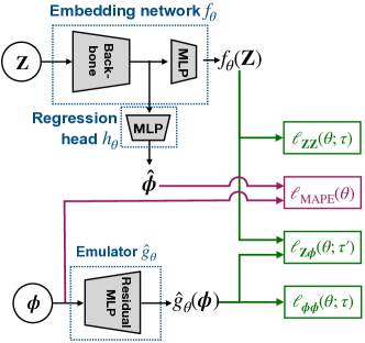
(a) Network setup

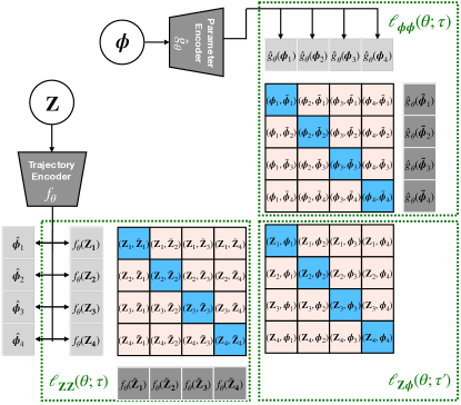
(b) Contrastive losses

Figure 1: The Embed & Emulate framework. (a) Components of our network and loss function. (b) We use three contrastive learning schemes. The bottom left block denotes the intra-trajecotry domain contrastive mechanism, the upper right denotes the intra-parameter domain contrastive learning, and the bottom right block shows inter-trajectory-parameter domains contrastive learning. Within each block, diagonals correspond to the dot product between the representations of positive trajectories pairs $(\mathbf{Z}_{i},{\tilde{\mathbf{Z}}}_{i})$, positive parameter pairs $({\boldsymbol{\phi}}_{i},\tilde{{\boldsymbol{\phi}}}_{i})$, and matched trajectory parameter pairs $(\mathbf{Z}_{i},{\boldsymbol{\phi}}_{i})$, which we aim to maximize. Off-diagonal pale pink blocks show similarities between the anchor point and the negatives examples, which we aim to minimize.

Intra-parameter domain contrastive loss: In order to fully exploit data potential within parameter space and better guide the learning of the representation and preserve similarities within the parameter space, we add an intra-parameter contrastive loss and find empirically that it helps accelerate the training process:

$$\ell_{{\boldsymbol{\phi}}{\boldsymbol{\phi}}}(\theta;\tau):=\frac{1}{n}\sum\limits_{i=1}^{n}-\log\frac{\exp\big{(}\langle\hat{g}_{\theta}({\boldsymbol{\phi}}_{i}),\hat{g}_{\theta}(\tilde{{\boldsymbol{\phi}}}_{i})\rangle/\tau\big{)}}{\sum\limits_{j=1}^{n}\exp\big{(}\langle\hat{g}_{\theta}({\boldsymbol{\phi}}_{i}),\hat{g}_{\theta}({\boldsymbol{\phi}}_{j})\rangle/\tau\big{)}},$$ (6)

where $\tilde{{\boldsymbol{\phi}}}$ is selected through data augmentation by perturbing ${\boldsymbol{\phi}}$ with small amount of noise (see Section B.1) or by finding nearest neighbors in the training set.

Regression head: Zimmermann et al. (2021) shows that under certain assumptions (see Section A.2), the feature encoder $f_{\theta}$ implicitly learns to invert the data generating process $H$ up to an affine transformation, implying we can estimate ${\boldsymbol{\phi}}$ via $h(f_{\theta}(\mathbf{Z}))$ for some linear function $h$. Inspired by their analysis, we add a regression head $h_{\theta}$ (a single fully-connected linear layer) in our framework, and we ensure the affine relationship between $h_{\theta}$ and $f_{\theta}$ by letting them share the same backbone up to the last layers before the output.

Unified training procedure: To this end, we formulate the final loss of our Embed & Emulate method as

$$\ell(\theta)=\lambda_{\mathbf{Z}\mathbf{Z}}\ell_{\mathbf{Z}\mathbf{Z}}(\theta;\tau)+\lambda_{{\boldsymbol{\phi}}{\boldsymbol{\phi}}}\ell_{{\boldsymbol{\phi}}{\boldsymbol{\phi}}}(\theta;\tau)+\lambda_{\mathbf{Z}{\boldsymbol{\phi}}}\ell_{\mathbf{Z}{\boldsymbol{\phi}}}(\theta;\tau^{\prime})+\lambda_{\rm MAPE}\ell_{\rm MAPE}(\theta),$$

where $\lambda_{\mathbf{Z}\mathbf{Z}},\lambda_{{\boldsymbol{\phi}}{\boldsymbol{\phi}}},\lambda_{\mathbf{Z}{\boldsymbol{\phi}}}$ and $\lambda_{\rm MAPE}$ control relative loss weights. We show our basic setup in Fig. 1(a) and loss framework in Fig. 1(b).

5 Experiments

We conduct a numerical case study on the multiscale Lorenz-96 (L96) model (Lorenz, 1996), which is a common test model for climate models with both “fast” (high-frequency) and “slow” (low-frequency) components and other geophysical applications (Majda and Harlim, 2012; Law and Stuart, 2012; Law et al., 2016; Brajard et al., 2020). It is a prototypical turbulent dynamical system “designed to mimic baroclinic turbulence in the midlatitude atmosphere” (Majda et al., 2010). Its dynamics exhibit strong energy-conserving non-linearities, and for some settings of ${\boldsymbol{\phi}}$, it can exhibit strong chaotic turbulence. Code is available at: https://github.com/roxie62/Embed-and-Emulate The governing equations of the L96 system are defined as follows:

$$\odv{\mathbf{X}^{k}_{t}}{t}=-\mathbf{X}^{k-1}_{t}(\mathbf{X}^{k-2}_{t}-\mathbf{X}^{k+1}_{t})-\mathbf{X}^{k}_{t}+F-hc\bar{\mathbf{Y}}^{k}_{t},$$

$$\frac{1}{c}\odv{\mathbf{Y}^{j,k}_{t}}{t}=-b\mathbf{Y}^{j+1,k}_{t}(\mathbf{Y}^{j+2,k}_{t}-\mathbf{Y}^{j-1,k}_{t})-\mathbf{Y}^{j,k}_{t}+\frac{h}{J}\mathbf{X}^{k}_{t},$$

where $\mathbf{X}_{t}\in\mathbb{R}^{K}$ denotes the slow variable at the $t$-th time stamp and $\mathbf{Y}_{t}\in\mathbb{R}^{KJ}$ denotes the fast variable. We use $\mathbf{Z}_{t}:=[\mathbf{X}_{t},\mathbf{Y}_{t}]\in\mathbb{R}^{K(J+1)}$ to denote the system state at the $t$-th time stamp. We choose $K=36$ and $J=10$ throughout experiments in this section, as in Schneider et al. (2017).

We set our baseline following Schneider et al. (2017). Within the EnKI framework, they use Runge-Kutta Dormand and Prince (1980) to compute the forward model $H$ and optimize (1). After analyzing the physics information of the L96 system, they define the moment function as: $m(\mathbf{Z}):=[\langle\mathbf{X}\rangle_{T},\langle\bar{\mathbf{Y}}\rangle_{T},\langle\mathbf{X}^{2}\rangle_{T},\langle\mathbf{X}\bar{\mathbf{Y}}\rangle_{T},\langle\bar{\mathbf{Y}}^{2}\rangle_{T}]$, where $\langle\cdot\rangle_{T}$ denotes an empirical average over $T$ time steps, $\bar{\mathbf{Y}}$ denotes an average across the $J$ $\mathbf{Y}$ channels, $\langle\bar{\mathbf{Y}}\rangle_{T}=(1/JT)\sum_{t=1}^{T}\sum_{j=1}^{J}\mathbf{Y}_{t}^{j,k}\in\mathbb{R}^{K}$, and other quantities are computed similarly (see details in Section B.1). $m(\mathbf{Z}_{t})\in\mathbb{R}^{5K}$. For the SBI methods, to suit the scenario we care about, i.e., estimating multiple $\boldsymbol{\phi}_{i}$ for multiple different observations $\mathbf{Z}_{i}$ at test time, we compare with the non-adaptive counterpart of the algorithms referenced in these papers. For instance, we set the round number of SNL+ (Chen et al., 2020b) to be one. And use the fixed training dataset for SNL+ and NPE-C (Greenberg et al., 2019).

We conduct experiments and demonstrate the efficacy when measuring (1) the accuracy of averaged point estimates, (2) the accuracy of uncertainty quantification, (3) the empirical computational complexity. For all of our experiments (including SNL+ and NPE-C), we use ResNet-34 (He et al., 2016) as the backbone of the trajectory encoder. We apply average pooling at the last layer to generate a 512-d hidden vector. For contrastive learning, we project the 512-d hidden vector into a 128-d feature vector as the output of the trajectory encoder. For the regression head, we map the 512-d hidden vector to a 4-d parameter vector. It is important to note that activation functions are not used in the regression head to ensure an affine mapping between two projections. We parameterize the emulator network with a ResNet backbone, and to enhance the representation power of the network, we use five residual connection blocks (see Section B.2). We find this increases the alignment between the two representation spaces. Within each skip block, there is a residual connection between the input layer and the output. The implementation details for training are shown in Section B.1.

5.1 Higher quality estimates with lower sample cost

In this section, we evaluate our method with different training sizes in the perfect-model setting where no noise is injected in observations. These experiments demonstrate the usefulness of our method in realistic scenarios where forward models are prohibitively expensive and only limited quantities of training data are available.

We train our Embed & Emulate method and the supervised regression baselines when the training size equals $500$ and $1,000$. The training samples are sampled uniformly from ${\boldsymbol{\phi}}_{\min}=[F_{\min},h_{\min},c_{\min},b_{\min}]=[-5,0,0.1,0]$ to ${\boldsymbol{\phi}}_{\max}=[F_{\max},h_{\max},c_{\max},b_{\max}]=[20,5,25,25]$, and each simulation is of length 100, with $dt=0.1$. We then sample 200 testing samples uniformly from a narrower range of $[-3,0.5,2,2]$ to $[18,4.5,23,23]$. As assumed in Schneider et al. (2017), each testing sample is of length $1,000$, with $dt=0.1$. The EnKI prior used for baselines (i.e. minimizing (1)) is a Gaussian distribution with means at the middle of the range of the testing instances, diagonal covariance matrix, and variances broad enough that all test samples are within $2\sigma$ of the mean, denoted $p_{{\boldsymbol{\phi}},{\rm fixed}}$ (see Section B.1). Within the context of the Embed & Emulate approach, we adopt an empirical Bayes approach: for each test instance, we compute $\hat{\boldsymbol{\phi}}$ using the regression head and use these values as the prior means when using EnKI to minimize (4); we denote this prior $p_{{\boldsymbol{\phi}},{\rm empB}}$. The impact of the empirical Bayes approach is explored in Section 5.3.

$n$		$F$ $\downarrow$	$h$ $\downarrow$	$c$ $\downarrow$	$b$ $\downarrow$
0	EnKI w/o Learning	15.48 (3.77)	0.86 (0.20)	40.45 (13.39)	4.60 (0.60)
500	$h_{\theta}$ w/ Embed & Emulate	11.19 (3.65)	3.18 (1.60)	15.52 (6.24)	8.57 (2.17)
	EnKI w/ Embed & Emulate	10.94 (4.07)	3.74 (2.26)	16.09 (6.41)	8.84 (2.93)
	Supervised Regression	11.97 (3.10)	4.07 (2.24)	17.04 (5.88)	9.07 (2.74)
	NPE-C	15.51 (4.52)	5.94 (2.59)	23.54 (8.16)	9.42 (3.70)
	SNL+	36.88(19.93)	48.71 (30.69)	57.45 (28.59)	23.45 (17.62)
1000	$h_{\theta}$ w/ Embed & Emulate	6.30 (1.86)	2.07 (1.31)	9.34 (3.71)	5.51 (1.74)
	EnKI w/ Embed & Emulate	6.59 (2.14)	2.36 (1.54)	9.38 (4.02)	5.54 (2.35)
	Supervised Regression	7.57 (1.78)	3.08 (1.54)	11.46 (3.29)	6.64 (2.19)
	NPE-C	11.29 (3.54)	5.62 (2.29)	16.32 (6.53)	6.81 (2.38)
	SNL+	33.29(19.68)	49.05 (27.75)	48.17 (23.90)	25.40 (16.03)

Table 1: Averaged MAPE (MdAPE, median absolute percentage error) for varying training size of different methods for 200 test samples. We compare Embed & Emulate w/ regression head ($h_{\theta}$) and Embed & Emulate plugged into EnKI to supervised regression, NPE-C (Greenberg et al., 2019), SNL+ (Chen et al., 2020b), and a classical numerical solver (Runge-Kutta) plugged into EnKI to minimize (1). The example illustrates that Embed & Emulate is able to achieve a lower error than both the EnKI approach based on a fixed moment vector objective and classical numerical solver (Schneider et al., 2017) and a straightforward supervised regression approach that is unable to produce uncertainty estimates.

	Training data generation	Training time	200 test runs	Total time (train + test)
EnKI w/o Learning	0.0	0.0	8,000.0	8,000 (5.5 d)
$h_{\theta}$ w/ Embed & Emulate	21.0	72.0	1.0	94.0 (1.57 h)
EnKI w/ Embed & Emulate	21.0	72.0	2.0	95.0 (1.58 h)
Supervised Regression	21.0	59.0	1.0	81.0 (1.35 h)
NPE-C	21.0	72.0	2.0	95.0 (1.58 h)
SNL+	21.0	73.0	400.0	494.0 (8.23 h)

Table 2: Empirical computational time for different stages of different methods ($n=1,000$). Reported in minutes, total time for Embed & Emulate, the supervised regression, or NPE-C are $1.19\%$ of EnKI with Runge-Kutta. All neural approaches are trained with 4 GPUs and tested with 1 GPU. Both training data generation and EnKI w/o Learning are run with 32 CPU Cores.

We first evaluate the accuracy of point estimates using the mean and median absolute percentage error (MAPE and MdAPE), see Section B.1. In Table 1 and Table 2, we see that Embed & Emulate evaluated with the regression head ($h_{\theta}$) and EnKI guarantees similar performance in terms of averaged accuracy. However, the regression head ($h_{\theta}$) is slightly better, which may be explained by our empirical observation that when estimates from $h_{\theta}$ with Embed & Emulate are far from the true parameter values, then using this estimate as the prior mean for EnKI can worsen the estimate. Despite this challenge, the EnKI has the advantage of providing uncertainty estimates, which are discussed below and reflected in Table 3.

Compared with other methods, it is clear that Embed & Emulate yields a significant improvement in accuracy, especially for the parameter affecting high-frequency dynamics (e.g., $c$). In particular, NPE-C (Greenberg et al., 2019) performs worse with a smaller training set size ; SNL+ (Chen et al., 2020b) using MCMC or rejection sampling suffers from increasing evaluation time as the number of test samples increases. Moreover, when compared to the classical method of running EnKI using a predefined moment function and expensive numerical solvers, Embed & Emulate yields better performance in terms of accuracy and computation time. Last, our Embed & Emulate framework also performs well relative to supervised regression for smaller training sets.

We then evaluate our results based on the continuous ranked probability score (CRPS) (Hersbach, 2000; Zamo and Naveau, 2018; Pappenberger et al., 2015). CRPS is an important metric used in quantifying uncertainty (e.g., in weather forecasts). It measures the accuracy of estimated posterior distributions and is defined as

$${\rm CRPS}(C,{\boldsymbol{\phi}}_{*j})=\int^{\infty}_{-\infty}(C(y_{j})-U(y_{j}-{\boldsymbol{\phi}}_{*j}))^{2}{\rm d}y_{j},$$

where $\boldsymbol{\hat{\phi}}_{*j}$ represents the $j$-th component of the estimate parameter vector, ${\boldsymbol{\phi}}_{*j}$ represents the $j$-th component of the true parameter vector, $C$ is the cumulative density function of the ensemble estimates with $C(y)=P({\boldsymbol{\phi}}_{*j}\leq y)$, and $U$ is the Heaviside step function. For a deterministic estimate from supervised regression, CRPS is equal to the mean absolute error (MAE). Table 3 shows that Embed & Emulate achieves high-accuracy estimates of uncertainty.

$n$		$F$ $\downarrow$	$h$ $\downarrow$	$c$ $\downarrow$	$b$ $\downarrow$
0	EnKI w/o Learning	0.910	0.019	2.443	0.393
500	$h_{\theta}$ w/ Embed & Emulate	0.698	0.076	1.715	0.824
	EnKI w/ Embed & Emulate	0.615	0.073	1.561	0.720
	Supervised Regression	0.707	0.104	1.785	0.917
	NPE-C	0.844	0.106	2.117	0.853
	SNL+	1.399	0.616	2.426	1.822
1000	$h_{\theta}$ w/ Embed & Emulate	0.412	0.049	0.992	0.453
	EnKI w/ Embed & Emulate	0.360	0.042	0.829	0.394
	Supervised Regression	0.478	0.078	1.242	0.650
	NPE-C	0.593	0.096	1.389	0.564
	SNL+	1.304	0.595	2.010	1.763

Table 3: Continuous Ranked Probability Score (CRPS) evaluated on 200 test samples. The errors of the uncertainty estimates are almost always lower for Embed & Emulate than for an EnKI method using a classical numerical solver. And compared to neural methods, EnKI with Embed & Emulate yields significant improvements over a supervised regression which cannot quantify uncertainty, defeats the simulation-based inference models NPE-C (Greenberg et al., 2019) and SNL+ (Chen et al., 2020b) which relies on sequential sampling. Moreover, it’s clear that Embed & Emulate evaluated with EnKI provides more accurate uncertainty estimates than point-wise estimates from the regression head ($h_{\theta})$ trained with Embed & Emulate.

5.2 Visualizing uncertainty with noisy observations

In this subsection, we go beyond the perfect-model setting and evaluate our method in the realistic scenarios where observations are noisy and obtained through: $\mathbf{Z}=H({\boldsymbol{\phi}})+\boldsymbol{\eta}$, where $\boldsymbol{\eta}\sim\mathcal{N}(0,r\boldsymbol{\Gamma})$, where $\boldsymbol{\Gamma}$ is the temporal covariance of the trajectory $\mathbf{Z}$, and $r$ is a scaling value. Specifically, we set ${\boldsymbol{\phi}}=[10,1,10,10]$ following Schneider et al. (2017) to ensure we are in the chaotic regime. We use model trained with $n=4,000$ data samples and compare the results obtained in both the noiseless and noisy cases. For this visualization, both methods use the fixed prior from Section 5.1 based on the range of test values, so any differences observed are not caused by differences in the prior, but rather differences in the choice of objective and the method of computing the forward model.

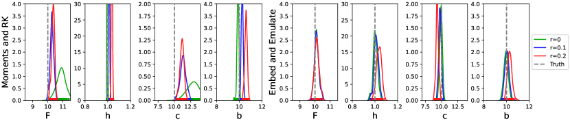
Figure 2: Impact of observation noise. Reconstructed posterior distributions, comparing a classical numerical solver (Runge-Kutta) plugged into EnKI to minimize (1) (left) with Embed & Emulate (right). Both variants of EnKI are run for 70 iterations with 100 particles. The green line shows the noise-free case, the blue shows the noisy case when $r=0.1$, and the red shows the noisy case when $r=0.2$. We see here that our proposed Embed & Emulate method (right column) produces posterior estimates that are consistent over a range of noise levels, while the baseline EnKI approach using a pre-defined embedding corresponding to a moments vector is much more sensitive to variations in $r$.

As shown in Fig. 2, Embed & Emulate is more robust to noise than the baseline method with numerical solvers and predefined moments. Reconstructed posterior distributions learned with Embed & Emulate in Fig. 2 are more consistent with increasing noise levels, especially for the parameters $F$ and $b$.

5.3 Ablation study: role of the regression head

In this section, we empirically verify the utility of the regression head $h_{\theta}$ in our Embed & Emulate framework. We use $n=4000$ training samples in two settings: first, we use the full Embed & Emulate model of Section 5.1; second, we discard the regression head (i.e. fix $h_{\theta}=0$) while keeping intra- and inter-domain contrastive losses. For both trained models, we run the EnKI. We run the EnKI using components from the Embed & Emulate framework for two choices of prior: first, we use $p_{{\boldsymbol{\phi}},{\rm fixed}}$, and second, we use $p_{{\boldsymbol{\phi}},{\rm empB}}$. Note the empirical Bayes prior is only possible with the regression head. These priors are detailed in Section 5.1 and Section B.1.

Table 4 shows that having the regression component of the loss complement the contrastive losses yields a substantial improvement in parameter estimation accuracy using Embed & Emulate. In other words, explicitly training the embedding function and emulator for the parameter estimation task yields an emulator that is far more accurate during parameter estimation than training a generic embedding and generic emulator. Furthermore, this table illustrates the efficacy of our empirical Bayes procedure – i.e., using our learned regressor to alter the prior used by EnKI. The medians are slightly improved while the means are strongly improved, suggesting that the empirical Bayes procedure is particularly helpful in the tails.

	$F$ $\downarrow$	$h$ $\downarrow$	$c$ $\downarrow$	$b$ $\downarrow$
(a) No regression head ($p_{{\boldsymbol{\phi}},{\rm fixed}}$)	16.75 (2.62)	6.02 (1.63)	22.16 (6.35)	6.60 (1.86)
(b) Embed & Emulate ($p_{{\boldsymbol{\phi}},{\rm fixed}}$)	8.39 (1.12)	1.77 (0.82)	15.82 (1.61)	3.85 (0.91)
(c) Embed & Emulate ($p_{{\boldsymbol{\phi}},{\rm empB}}$)	3.39 (1.03)	1.21 (0.76)	4.53 (1.52)	3.02 (0.90)

Table 4: Ablation study of regression head: Average MAPE (MdAPE, median absolute percentage error) over 200 test instances for estimating ${\boldsymbol{\phi}}$ by minimizing (4) in three different settings: (a) $f_{\theta}$ and $\hat{g}_{\theta}$ correspond to a generic emulator trained without the regression loss $\ell_{\rm reg}$ and the original prior $p_{{\boldsymbol{\phi}},{\rm fixed}}$; (b) $f_{\theta}$ and $\hat{g}_{\theta}$ correspond to the emulator learned with our Embed & Emulate framework and the original prior $p_{{\boldsymbol{\phi}},{\rm fixed}}$; and (c) $f_{\theta}$ and $\hat{g}_{\theta}$ correspond to the emulator learned with our Embed & Emulate framework and the empirical Bayes prior $p_{{\boldsymbol{\phi}},{\rm empB}}$. This experiment shows that having the regression component of the loss complement the contrastive losses yields a substantial improvement in parameter estimation accuracy using Embed & Emulate.

6 Conclusions

The proposed Embed & Emulate framework trains an emulator of a complex simulation to facilitate parameter estimation. Unlike generic emulation methods, which can lead to poor parameter estimates and require expert domain knowledge to construct, our method (a) leverages a contrastive learning framework coupled with a regression head to jointly learn a low-dimensional embedding of simulator outputs that can be used to construct an objective function for parameter estimation and (b) yields an emulator that can be used within an optimization framework such as the EnKI to produce accurate parameter estimates in 1.19% of the computation time of an approach using classical numerical methods, even accounting for the time required to generate training samples. We explore our approach in the context of earth system modeling as described by Schneider et al. (2017) and Cleary et al. (2021) and hypothesize that these tools can facilitate improved climate forecasts that account for uncertainties and cover the full range of possible outcomes. The social impacts of improved climate forecasting are positive if acted upon. While learned emulators are gaining in popularity, we as a community still know little about which systems are more or less challenging to emulate or how to design task-specific emulators more generally. There are further opportunities for exploring emulators for parameter estimation using optimization frameworks beside the EnKI.

Appendix A Algorithms and analysis

A.1 Ensemble Kalman Inversion

Ensemble Kalman Inversion (EnKI) gained its popularity in addressing Bayesian inverse problems since its proposal [Iglesias et al., 2013]. It is a derivative-free optimization method for objective functions of the form [Chada et al., 2020] :

$$J_{\rm DM}({\boldsymbol{\phi}}):=\frac{1}{2}\lVert\mathbf{y}_{\rm{measure}}-g({\boldsymbol{\phi}})\rVert^{2}_{\mathbf{R}},$$ (7)

where $\mathbf{y}_{\rm{measure}}$ is the measured data, $g$ is a given map and $\mathbf{R}$ is a symmetric positive definite matrix representing the data measurement precision (we explain how different approaches in our paper using different $\mathbf{y}_{\rm measure}$ and $\mathbf{R}$ below).

The EnKI estimates a posterior distribution of ${\boldsymbol{\phi}}$, which is approximated using an ensemble of particles. At each iteration, the EnKI consists of two steps: the prediction step and the analysis step. In the prediction step, we apply the forward model $g$ to each particle of the ensemble. In the analysis step, each particle is updated by using artificially perturbed observations and forward-mapped particles. The EnKI is summarized in Algorithm 1.

Algorithm 1 EnKI ($\mathbf{y}_{\rm{measure}},g,p_{\boldsymbol{\phi}},\alpha,\mathbf{R},M,N)$

0:  Data $\mathbf{y}_{\rm{measure}}$, forward model $g$, prior distribution $p_{\boldsymbol{\phi}}$, step size $\alpha$, variance $\mathbf{R}$, ensemble size $M$, number of iterations $N$. Initialize: $\{\boldsymbol{\hat{\phi}}^{(0,m)}\}_{m=1}^{M}$ sampled from the prior distribution $p_{\boldsymbol{\phi}}$.

1:  for $i=1,\cdots N$  do

2:     Prediction step: propagate the ensemble of particles to data space $\{g\big{(}\boldsymbol{\hat{\phi}}^{(i,m)}\big{)}\}_{m=1}^{M}$ by applying the forward model $g$ $M$ times. From the ensemble, calculate the empirical means and covariance matrices:

$$\hbox to0.0pt{\hskip 0.47916pt\leavevmode\hbox{\set@color$\overline{\hbox{}}$}\hss}{\leavevmode\hbox{\set@color${\boldsymbol{\phi}}$}}^{i}=\frac{1}{M}\sum_{m=1}^{M}{\boldsymbol{\phi}}^{(i,m)},\text{ }\hbox to0.0pt{\hskip 0.06422pt\leavevmode\hbox{\set@color$\overline{\hbox{}}$}\hss}{\leavevmode\hbox{\set@color$g$}}^{i}=\frac{1}{M}\sum_{m=1}^{M}g\big{(}\boldsymbol{\hat{\phi}}^{(i,m)}\big{)},$$

$$\mathbf{C}^{i}_{{\boldsymbol{\phi}}g}=\frac{1}{M}\sum_{m=1}^{M}\Big{(}\boldsymbol{\hat{\phi}}^{(i,m)}_{i}-\hbox to0.0pt{\hskip 0.47916pt\leavevmode\hbox{\set@color$\overline{\hbox{}}$}\hss}{\leavevmode\hbox{\set@color${\boldsymbol{\phi}}$}}^{i}\Big{)}\otimes\Big{(}g\big{(}\boldsymbol{\hat{\phi}}^{(i,m)}\big{)}-\hbox to0.0pt{\hskip 0.06422pt\leavevmode\hbox{\set@color$\overline{\hbox{}}$}\hss}{\leavevmode\hbox{\set@color$g$}}^{i}\Big{)},$$

$$\mathbf{C}^{i}_{gg}=\frac{1}{M}\sum_{m=1}^{M}\Big{(}g\big{(}\boldsymbol{\hat{\phi}}^{(i,m)}\big{)}-\hbox to0.0pt{\hskip 0.06422pt\leavevmode\hbox{\set@color$\overline{\hbox{}}$}\hss}{\leavevmode\hbox{\set@color$g$}}^{i}\Big{)}\otimes\Big{(}g\big{(}\boldsymbol{\hat{\phi}}^{(i,m)}\big{)}-\hbox to0.0pt{\hskip 0.06422pt\leavevmode\hbox{\set@color$\overline{\hbox{}}$}\hss}{\leavevmode\hbox{\set@color$g$}}^{i}\Big{)},$$

3:     Analysis step: calculate the Kalman gain matrix

$$\mathbf{K}^{i}=\mathbf{C}^{i}_{{\boldsymbol{\phi}}g}(\mathbf{C}^{i}_{gg}+\alpha^{-1}\mathbf{R})^{-1},$$

artificially perturb the data $\mathbf{y}_{\rm{measure}}^{(i,m)}=\mathbf{y}_{\rm{measure}}+\eta^{(i,m)}$ where $\eta^{(i,m)}\sim\mathcal{N}(0,\alpha^{-1}\mathbf{R})$, and update the ensemble of particles:

$$\boldsymbol{\hat{\phi}}^{(i+1,m)}=\boldsymbol{\hat{\phi}}^{(i,m)}+\mathbf{K}^{i}\Big{(}\mathbf{y}_{\rm{measure}}^{(i,m)}-g\big{(}\boldsymbol{\hat{\phi}}^{(i,m)}\big{)}\Big{)},1\leq m\leq M.$$

4:  end for

4:  $\{\boldsymbol{\hat{\phi}}^{(N,m)}\}$

When using Embed & Emulate to minimize the objective function (4), $\mathbf{y}_{\rm{measure}}$ corresponds to the embedding of the raw trajectory $f_{\theta}(\mathbf{Z})$, the forward model $g$ corresponds to the emulator $\hat{g}_{\theta}$, and $\mathbf{R}$ corresponds to an identity matrix. When using the baseline method to minimize the objective function (1), $\mathbf{y}_{\rm{measure}}$ corresponds to the moment vector $m(\mathbf{Z})$, $g$ corresponds to the $m\circ H$ where $H$ is computed using Runge-Kutta method, and $\mathbf{R}$ is a diagonal matrix with $j$-th diagonal entry $\mathbf{R}_{j,j}:={\rm Var}[m(\mathbf{Z})_{j}]$.

A.2 Contrastive learning and inverse problems

In this section, we briefly reviewed the assumptions and results of Zimmermann et al. [2021] and explain how we relate the analysis to our work in addressing the parameter estimation problem.

Recent literature studies the reason why contrastive learned representations can be successfully extended to multiple downstream tasks [Arora et al., 2019, Wang and Isola, 2020, Zimmermann et al., 2021]. Among them, a recent work from Zimmermann et al. [2021] points out that under certain assumptions, the representations $f_{\theta}$ learned in the contrastive framework to minimize $\ell_{\mathbf{Z}\mathbf{Z}}(\theta;\tau)$ (shown in (3)) inverts the underlying data generating process $H^{-1}(\mathbf{Z})$ of observed data up to an affine transformation.

Assumptions

Zimmermann et al. [2021] firstly make assumptions on the data generating process. They assume the generator $H:\Phi\rightarrow\mathcal{Z}$ is an injective function with $\Phi\in\mathbb{S}^{k-1}$ in a unit hypersphere and the distribution of ${\boldsymbol{\phi}}\in\Phi$ is uniform. Second, they assume the conditional distribution $p(\tilde{{\boldsymbol{\phi}}}|{\boldsymbol{\phi}})$ of a “positive parameter” $\tilde{{\boldsymbol{\phi}}}$ given ${\boldsymbol{\phi}}$ is a von Mises-Fisher (vMF) distribution with $p(\tilde{{\boldsymbol{\phi}}}|{\boldsymbol{\phi}})=c_{p}^{-1}\exp(\kappa\langle\tilde{{\boldsymbol{\phi}}},{\boldsymbol{\phi}}\rangle)$ where $c_{p}$ is the normalizing constant and $\kappa$ is the concentration parameter. Third, they assume the learned representation $f_{\theta}:\mathcal{Z}\rightarrow\mathbb{S}^{k-1}$ is in the unit hypersphere where the dimension of the representation is equal to the dimension of the parameters. They further assume the learned conditional distribution of $\tilde{{\boldsymbol{\phi}}}$ given ${\boldsymbol{\phi}}$ with the contrastive trained neural network is a vMF distribution with $q_{\theta}(\tilde{{\boldsymbol{\phi}}}|{\boldsymbol{\phi}})=C_{q}({\boldsymbol{\phi}})^{-1}\exp(\langle f_{\theta}(H(\tilde{{\boldsymbol{\phi}}}),f_{\theta}(H({\boldsymbol{\phi}}))/\tau\rangle)$ where $C_{q}({\boldsymbol{\phi}})$ is the partition function.

In the context of the parameter estimation problem of this paper, the relationship proved by Zimmermann et al. [2021], that $f_{\theta}(\mathbf{Z})=AH^{-1}(\mathbf{Z})=A{\boldsymbol{\phi}}$ where $A$ is a full rank matrix, is clearly a desirable property as, if $A$ were known, we could simply invert $A$ to obtain an unbiased estimate of ${\boldsymbol{\phi}}$. Empirically, we find that directly adding a linear regression head on top of $f_{\theta}$ (which effectively serves as a mechanism for learning $A^{-1}$; see Fig. 1) provides faster convergence and better performance (as shown in Section 5.3).

Appendix B Implementation details

B.1 Experiment details

Lorenz 96 dataset

Initial conditions of the ODE/PDE systems affect the values of dynamical variables at future times. To better fit in real-world scenarios, we simulate the training data used for Embed & Emulate and the supervised regression, as well as the testing data used for evaluations of all methods, with random initial conditions sampled from the normal distributions. During EnKI evaluations of the baseline we are required to specify initial conditions. We follow Schneider et al. [2017] and set the initial conditions of all simulations in the EnKI evaluations as random samples drawn from the observation. Note that, unlike the baseline method, Embed & Emulate directly learns the structural embeddings of ${\boldsymbol{\phi}}$ and does not require initial conditions. Beyond the setup of initial conditions, there are two stages to generate our train and test data. In the first stage, we generate a collection of ${\boldsymbol{\phi}}_{i}$, and for each one, we run a Runge-Kutta solver to compute a corresponding $\mathbf{Z}_{i}$. In the second stage, we filter out some of the $\{{\boldsymbol{\phi}}_{i},\mathbf{Z}_{i}\}$ generated during the first stage –whenever the Runge-Kutta iterations are unsuccessful, generating NaN values, and whenever the $\mathbf{Z}_{i}$ are degenerate, resulting in a standard deviation below 5e-5.

Data processing

(a)Trajectory cropping: during the training of Embed & Emulate and the supervised regression, we randomly crop a collection of length-250 trajectories from length-1000 trajectories, where each crop $\mathbf{Z}_{\rm{crop}}\in\mathbb{R}^{250\times 396}$. (b) “positive” data selection: Embed & Emulate trained with contrastive learning objectives tries to pull “anchor” data $\mathbf{Z}$ (or ${\boldsymbol{\phi}}$) towards “positive” data ${\tilde{\mathbf{Z}}}$ in (3) (or $\tilde{{\boldsymbol{\phi}}}$ in (6)) and at the same time push “negative” data away. To identify a “positive” trajectory ${\tilde{\mathbf{Z}}}$ (or parameter $\tilde{{\boldsymbol{\phi}}}$), we use a two-step approach. First, we select it in a supervised manner by measuring the distance between the “anchor” data $\mathbf{Z}_{i}$ (or ${\boldsymbol{\phi}}_{i}$) and a sample $\mathbf{Z}_{j}$ (or ${\boldsymbol{\phi}}_{j}$) in the parameter space. We find the index $\tilde{i}$ of the nearest neighbor of the “anchor” data in the parameter space with $\tilde{i}:=\arg\min_{i\neq j}\delta({\boldsymbol{\phi}}_{i},{\boldsymbol{\phi}}_{j})$, where $\delta$ is a metric function defined as: $\delta({\boldsymbol{\phi}}_{i},{\boldsymbol{\phi}}_{j}):=\frac{1}{2}\big{\{}{\rm APE}({\boldsymbol{\phi}}_{i};{\boldsymbol{\phi}}_{j})+{\rm APE}({\boldsymbol{\phi}}_{j};{\boldsymbol{\phi}}_{i})\big{\}}$ (see $\rm{APE}$ in Section B.3). However, since the training data is sampled from finite grids with limited size, the distance between the “anchor” data and its nearest neighbor $\delta({\boldsymbol{\phi}}_{i},{\boldsymbol{\phi}}_{\tilde{i}})$ could be very large. We apply a threshold filter and only accept a candidate nearest neighbor as “positive” data when the empirical distance $\delta({\boldsymbol{\phi}}_{i},{\boldsymbol{\phi}}_{\tilde{i}})$ is below some threshold (e.g., $0.45$ for $n=500$, $0.4$ for $n=1,000$ and $4,000$ ). Second, for the cases where no sample passes the threshold filter, we set ${\tilde{\mathbf{Z}}}$ and $\tilde{{\boldsymbol{\phi}}}$ in two different ways. For ${\tilde{\mathbf{Z}}}$, we simply set it in an unsupervised way by randomly making another crop on $\mathbf{Z}_{i}$. For $\tilde{{\boldsymbol{\phi}}}$, we set it by randomly adding a small amount of noise on ${\boldsymbol{\phi}}_{i}$ with $\tilde{{\boldsymbol{\phi}}}_{ij}:={\boldsymbol{\phi}}_{ij}+\xi{\boldsymbol{\phi}}_{ij},j=1,2,3,4$ with a certain probability (e.g., $50\%$), where $\xi$ is a normal variable with mean 0 and a small standard deviation (e.g., 0.04).

Training Hyperparameters

We train Embed & Emulate and the supervised regression using the AdamW optimizer. For both methods, we linearly warm up the learning rate to 0.01 at the beginning of the training and then gradually decay the learning rate with a cosine decay scheduler. We use $\lambda=$1e-5 for weight decay. We train NPE-C [Greenberg et al., 2019] and SNL+ [Chen et al., 2020b] with learning rate 1e-4 and 5e-4 as we find lower learning rate leads to better performance. We train all the methods with $1,000$ epochs. We use batch size $1000$ for large sized training data with $n\geq 1,000$. For the small size training data with $n=500$, we set it as $500$.

Temperature values in contrastive learning balance the influence between barely distinguishable samples and easily distinguishable “negative” samples [Ravula et al., 2021]. They are commonly chosen to be less than one where smaller values indicate a larger influence of barely distinguishable “hard” samples. For Embed & Emulate, we initialize the temperature values $\tau$ in (3) and (6) and $\tau^{\prime}$ in (5) at $0.15$. We keep $\tau$ and $\tau^{\prime}$ fixed at $0.15$ for the first $500$ epochs to make sure “hard” samples get large gradients and are updated sufficiently. We then adopt the “heating-up” strategy from Zhang et al. [2018] and linearly increase $\tau$ in (3) and (6) to 0.5 to increase the impact of “easier” samples. We keep $\tau^{\prime}$ in (5) fixed all the time so that the learned emulator $\hat{g}_{\theta}$ is capable of distinguishing embeddings of “hard” samples from the embedding network $f_{\theta}$, and vice versa.

In training a contrastive learning target, we usually need sufficient amount of “negative” samples to approximate the uniform repulsion. We follow He et al. [2020] and construct a first-in-first-out queue with a rolling updating scheme. Practically, the memory bank size should be no less than the training size. In our experiments, we set the size of the memory bank as $5,000$ when the training size $n=4,000$; the size of the memory bank as $2,000$ when the training size $n=1,000$; and the size of the memory bank as $1,500$ when the training size $n=500$.

All the hyperparameters are chosen using a grid search with a reserved validation set consisting of 5 samples. The range of values searched over are as follows:

• The initialized learning rates for Embed & Emulate and the supervised regression were selected from the set $\{0.001,0.01\}$.

• The initialized temperature values of $\tau$ in (3) and (6) and $\tau^{\prime}$ in (5) were selected from the set $\{0.10,0.15,0.20\}$. The heated up maximum value of $\tau$ in (3) and (6) were selected from the set $\{0.1,0.2,0.3,0.4,0.5\}$.

Priors Initialization of the EnKI

As Schneider et al. [2017], for the initialization of the EnKI prior, we use a normal prior for $({\boldsymbol{\phi}}_{1},{\boldsymbol{\phi}}_{2},{\boldsymbol{\phi}}_{4})=(F,h,b)$ and a log-normal prior for ${\boldsymbol{\phi}}_{3}=c$ in order to enforce positivity. For the baseline method minimizing (1) in Section 5.1 and Section 5.2, we use a fixed prior $p_{{\boldsymbol{\phi}},{\rm fixed}}$. For the normal variables, we choose the mean at the middle of the range of testing instances: $\mu_{{\boldsymbol{\phi}},{\rm fixed}}(F,h,b)=(7.5,2.5,12.5)$ and variances broad enough so that all test samples are within $2\sigma$ of the mean: $\sigma^{2}_{{\boldsymbol{\phi}},{\rm fixed}}(F,h,b)=(36.0,2.25,36.0)$. For the log-normal variable $\log c$, we set its mean $\mu_{{\boldsymbol{\phi}},{\rm fixed}}(\log c)=\log(11.5)$ and variance $\sigma^{2}_{{\boldsymbol{\phi}},{\rm fixed}}(\log c)=0.15$ (i.e., a mean value of $12.5$ for $c$). For Embed & Emulate, we can choose between the instance-wise prior $p_{{\boldsymbol{\phi}},{\rm empB}}$ and the fixed prior defined above. Specifically, we alter the mean of $p_{{\boldsymbol{\phi}},{\rm empB}}$ with the empirical estimate provided by the regression head and use a relatively small variance. $\sigma^{2}_{{\boldsymbol{\phi}},{\rm emp}}(F,h,b)=(18.0,1.125,18.0)$ for normal variables and $\sigma^{2}_{{\boldsymbol{\phi}},{\rm emp}}(\log c)=0.075$ for log-normal variable $c$.

Setup of the EnKI

For experiments in Section 5.1, we set the ensemble size $M=100$, step size $\alpha=0.3$ and iteration number $N=50$ for the baseline method with $p_{{\boldsymbol{\phi}},{\rm fixed}}$ and Embed & Emulate with $p_{{\boldsymbol{\phi}},{\rm empB}}$. For the study of noise impact in Section 5.2 when evaluating the baseline and Embed & Emulate, we use $p_{{\boldsymbol{\phi}},{\rm fixed}}$. For the ablation study in Section 5.3 when evaluating Embed & Emulate and no regression head contrastive learning with $p_{{\boldsymbol{\phi}},{\rm fixed}}$, we set a large ensemble size $M=10,000$ to prevent potential collapse in a local minimum and $N=100$ to ensure convergence. Arguably, this could slow down the computational times. However, empirically we only increased the time from $2$ seconds to $16$ seconds per instance, which is significantly lower than the times consumed by the baseline method.

Computational resources

Experiments of Embed & Emulate and the supervised regression were performed on a system with 4x Nvidia A40 GPUs, 2 AMD EPYC 7302 CPUs, and 128GB of RAM. The baseline methods and data generating process were performed on 2x Xeon Gold 6130 CPUs.

B.2 Network Architecture

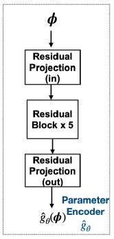
(a) Encoder network

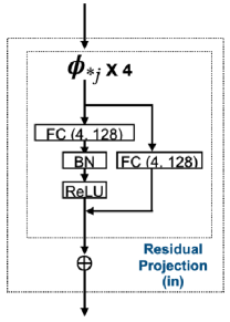
(b) Residual projection (in)

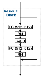
(c) Residual block

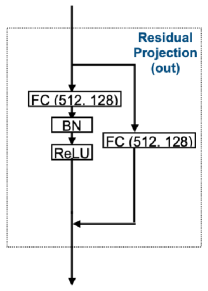
(d) Residual projection (out)

Figure 3: Architecture of emulator $\hat{g}_{\theta}$ of Embed & Emulate (a) The emulator network consists of one residual projection (in), three residual projection blocks, and one residual projection (out). (b) The residual projection (in) independently maps the $j$-th item of ${\boldsymbol{\phi}}$ into a high-dimensional (e.g., 128) latent representation, which is then concatenated (shown as the $\oplus$ operator) as a single vector as the output. (c) The residual block has the same input and output dimension. (4) The residual projection (out) projects a high-dimensional input latent vector into a low-dimensional embedding.

Emulator $\hat{g}_{\theta}$

To enhance the representation power of the emulator $\hat{g}_{\theta}$ and enlarge the alignment between two learned representation spaces, we design the emulator using residual blocks as in Fig. 3.

Embedding network $f_{\theta}$

We use Resnet34 [He et al., 2016] as the backbone of the trajectory branch of Embed & Emulate in Fig. 1(a) and the supervised regression. We apply average pooling at the last layer to generate a 512-d hidden vector. To respect the temporal periodic pattern of Lorenz 96, we replace the standard zero padding with the circular padding on the temporal axis. For the regression head $h_{\theta}$, we project the 512-d hidden vector into a 4-d output using only a single fully connected layer. For the embedding network, we project the 512-d hidden vector into a 128-d feature vector using a similar structured branch as projection residual (out) in Fig. 3(d) except that the residual block skips two layers instead of one.

B.3 Performance metrics

Absolute Percentage Error (APE)

: APE is used in selecting “positive” samples of Embed & Emulate and is calculated on pairs of training samples:

$${\rm APE}({\boldsymbol{\phi}}_{j};{\boldsymbol{\phi}}_{i})=\sum_{l=1}^{k}\frac{|{\boldsymbol{\phi}}_{il}-{\boldsymbol{\phi}}_{jl}|}{|{\boldsymbol{\phi}}_{il}+\epsilon|},$$ (8)

here $k$ is the dimension of ${\boldsymbol{\phi}}$, $i,j$ represent indexes of two data samples, and $\epsilon$ is a small value to address overflow issues.

Mean Absolute Percentage Error (MAPE)

MAPE is a measure of prediction accuracy over the entire testing data and is expressed as a ratio with the formula:

$${\rm MAPE}(\boldsymbol{\hat{\phi}}_{*j};{\boldsymbol{\phi}}_{*j})=\frac{1}{n}\sum_{i=1}^{n}\frac{|\boldsymbol{\hat{\phi}}_{ij}-{\boldsymbol{\phi}}_{ij}|}{|{\boldsymbol{\phi}}_{ij}|+\epsilon},$$ (9)

where $\boldsymbol{\hat{\phi}}_{*j}$ represents the $j$-th component of the estimate parameter vector, ${\boldsymbol{\phi}}_{*j}$ represents the $j$-th component of the true parameter vector (e.g., $[{\boldsymbol{\phi}}_{*1},{\boldsymbol{\phi}}_{*2},{\boldsymbol{\phi}}_{*3},{\boldsymbol{\phi}}_{*4}]=[F,h,c,b]$ for Lorenz 96), and $\epsilon$ is a small value to address overflow issues.

Continuous Ranked Probability Score(CRPS)

As described in Section 5.1, CRPS is a probability metric to evaluate the performance of a probabilistic estimation. CRPS is computed as a quadratic measurement of cumulative distribution function (CDF) between the predicted distribution $C$ and the empirical distribution of the observation. CRPS is defined as [Hersbach, 2000, Zamo and Naveau, 2018, Pappenberger et al., 2015]:

$${\rm CRPS}(C,{\boldsymbol{\phi}}_{*j})=\int^{\infty}_{-\infty}(C(y_{j})-U(y_{j}-{\boldsymbol{\phi}}_{*j}))^{2}{\rm d}y_{j},$$ (10)

where ${\boldsymbol{\phi}}_{*j}$ and $\boldsymbol{\hat{\phi}}_{*j}$ are defined above, $C$ is the CDF of the ensemble estimation with $C(y_{j})=P(\boldsymbol{\hat{\phi}}_{*j}\leq y_{j})$, and $U$ is the CDF of the Heaviside step function with $U(y_{j}-{\boldsymbol{\phi}}_{*j})=\mathbf{1}\{y_{j}\geq{\boldsymbol{\phi}}_{*j}\}$. Practically estimating $C$ is difficult since it has no analytic form. In our case, using EnKI with ensemble size $M$, we can estimate (10) using the empirical distribution calculated from the particles $\{\boldsymbol{\hat{\phi}}_{*j}^{(m)}\}_{m=1}^{M}$:

$${\rm CRPS}(C,{\boldsymbol{\phi}}_{*j})=-\frac{1}{2M^{2}}\sum_{m=1}^{M}\sum_{m^{\prime}=1}^{M}|\boldsymbol{\hat{\phi}}_{*j}^{(m)}-\boldsymbol{\hat{\phi}}_{*j}^{(m^{\prime})}|+\frac{1}{M}\sum_{m=1}^{M}|\boldsymbol{\hat{\phi}}_{*j}^{(m)}-{\boldsymbol{\phi}}_{*j}|.$$ (11)

B.4 Visualizing the objective functions

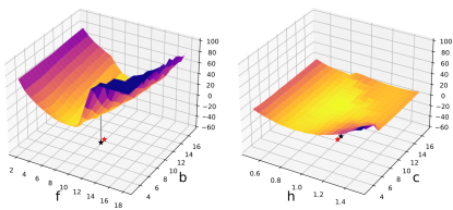
(a) Marginal heatmap of (1) using Runge-Kutta

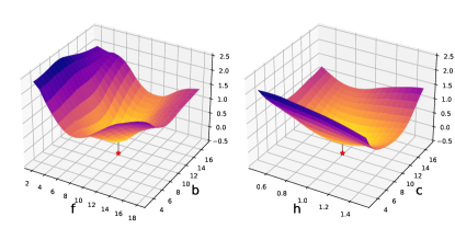
(b) Marginal heatmap of (4) using learned emulator.

Figure 4: Heatmap visualization showing values of objective functions. (a) the marginal heatmap of predefined moments objective function (1); and (b) the marginal heatmap of (4) with Embed & Emulate using learned emulator. The red stars in both plots show the locations of the true parameters, while the black stars show the locations of the points with the minimum function value. All objective values are greater or equal to zero, but we intentionally set the limit of $z$-axis to be negative for clear visualization of “star” points. $z$-axes between different marginal heatmaps using the same objective function are aligned with post-processing. Unlike the value of the objective function (4) are bounded between $[0,4]$, values of (1) have no upper bound and might contain extremely large numbers. For better visualization, we manually truncate values of (1) by a threshold number (e.g.,100) for better visualization.

In this section, we visualize the objective function of (1) with predefined moments function and Runge-Kutta and (4) of Embed & Emulate with emulator $f_{\theta}$ and $\hat{g}_{\theta}$. We use the same instance in Section 5.2 as the observation with the ground truth ${\boldsymbol{\phi}}=[10,1,10,10]$ and the noiseless $\mathbf{Z}$ is of length $10,000$. Fig. 4 shows the marginal heatmaps of the objective functions when holding two parameters fixed at the ground truth values and sampling the other two parameters uniformly in a fixed range. We can see that the objective function learned with Embed & Emulate can accurately reflect the dynamics in the parameter space with smooth curves. In contrast, the predefined objective function is insensitive to the parameter $c$ with a flat curve showing in the marginal heatmap of $(h,c)$ pairs.

Appendix C Further Experiments

In this section, we study the 1-d Kuramoto-Sivashinsky equation (KSE). Kuramoto-Sivashinsky equation is known for its chaotic dynamics and can be applied in describing a variety of physical phenomena, including flows in pipes, plasmas, chemical reaction dynamics, etc. [Hyman and Nicolaenko, 1986] The Kuramoto-Sivashinsky equation is a fourth-order partial differential equation with the form:

$$\pdv{\mathbf{V}^{x}_{t}}{t}+\lambda_{2}\pdv[order=2]{\mathbf{V}^{x}_{t}}{x}+\lambda_{4}\pdv[order=4]{\mathbf{V}^{x}_{t}}{x}+\lambda_{\rm nonlinear}\mathbf{V}^{x}_{t}\pdv{\mathbf{V}^{x}_{t}}{x}=0,$$

$$\text{and }\mathbf{V}^{x}_{t}=\mathbf{V}^{x+2L}_{t},$$

where $\mathbf{V}^{x}_{t}$ is the state of KSE, $\lambda_{2}$, $\lambda_{4}$ and $\lambda_{\rm nonlinear}$ are the coefficients of second-order derivative, fourth-order derivative and nonlinear term. In all, we define ${\boldsymbol{\phi}}:=[\lambda_{2},\lambda_{4},\lambda_{\rm nonlinear}]$, and our goal is to learn ${\boldsymbol{\phi}}$ from sequences of observations $\mathbf{V}\in\mathbb{R}^{T\times d}$.

Choosing the moments function

We choose the first order statistics of $\mathbf{V}$ to define the moments function: $m(\mathbf{V})=[\langle\mathbf{V}\rangle]$ where $\langle\cdot\rangle$ denotes empirical average over time. Note here we have tried multiple combinations of moments, including second-order and third-order statistics but found no choice of moments performs better than using only the first-order.

Preparation of dataset

We set $L=32$ and $d=256$ to ensure we are in a chaotic regime. Initial conditions are randomly sampled from a uniform range $[-\pi,\pi]$. All simulations performed here are completed with a Runge-Kutta 4-stage method as Pachev et al. [2021]. Training data are sampled uniformly for all three components of ${\boldsymbol{\phi}}$ ranging from $\min=0.1$ to $\max=10.0$ with length $T=400,dt=0.5$ and size $n=500$. 100 testing data are sampled in a narrower range from $\min=0.5$ and $\max=9.5$ with length 800 and $dt=0.5$.

Setup of the EnKI

We set the fixed Gaussian prior $p_{{\boldsymbol{\phi}},{\rm fixed}}$ with mean at the middle of the testing range and variance broader enough to cover all testing instances in $2\sigma$: $\mu_{\rm{\boldsymbol{\phi}}_{*j},fixed}=5,\sigma^{2}_{\rm{\boldsymbol{\phi}}_{*j},fixed}=6.25,j=1,2,3$. We use the same variance for $p_{{\boldsymbol{\phi}},{\rm empB}}$ and alter its mean with the empirical estimate provided by the regression head. For both baseline and Embed & Emulate, we set ensemble size $M=100$, iteration number $N=40$, step size $\alpha=0.3$.

Setup of the training

We train both Embed & Emulate and the supervised regression for 1,000 epochs. We set the memory bank size of Embed & Emulate for 1,000. We set the dimension of learned representation, i.e., $f_{\theta}(\mathbf{V})$ and $\hat{g}_{\theta}({\boldsymbol{\phi}})$ to be 120. We use the same learning rate and cosine decay scheduler. We initialize $\tau,\tau^{\prime}=0.1$, and linearly warm up $\tau^{\prime}$ from 500 to 900 epochs with the maximum value $0.6$.

	$\lambda_{2}\downarrow$	$\lambda_{4}\downarrow$	$\lambda_{\rm nonlinear}\downarrow$
(a) EnKI w/o Learning	34.73(25.44)	56.14 (38.27)	68.64(33.90)
(b) $h_{\theta}$ w/ Embed & Emulate	3.24 (1.56)	3.70 (1.68)	2.69 (1.45)
(c) EnKI w/ Embed & Emulate	3.48 (1.42)	3.29 (1.50)	3.30 (1.69)
(d) Supervised regression	3.27 (1.16)	3.34 (0.97)	3.14 (1.36)
(e) NPE-C	4.30 (2.14)	4.86 (2.59)	3.30 (1.83)

Table 5: Averaged MAPE (MdAPE, median absolute percentage error) over 100 test instances. (a) EnKI plugged in the Runge-Kutta solver and predefined moments function in minimizing (1); (b) Embed & Emulate with Regresssion head ($h_{\theta}$); and (c) EnKI plugged in our Embed & Emulate with the empirical Bayes prior $p_{{\boldsymbol{\phi}},{\rm empB}}$; (d) Supervised regression; (e) NPE-C [Greenberg et al., 2019].

	$\lambda_{2}\downarrow$	$\lambda_{4}\downarrow$	$\lambda_{\rm nonlinear}\downarrow$
(a) EnKI w/o Learning	1.14	1.50	1.47
(b) $h_{\theta}$ w/ Embed & Emulate	0.148	0.149	0.125
(c) EnKI w/ Embed & Emulate	0.121	0.101	0.114
(d) Supervised regression	0.149	0.124	0.150
(e) NPE-C	0.175	0.217	0.131

Table 6: Averaged continuous ranked probability score (CRPS) over 100 test instances. (a) EnKI plugged in the Runge-Kutta solver and predefined moments function in minimizing (1); (b) Embed & Emulate with Regresssion head ($h_{\theta}$); and (c) EnKI plugged in our Embed & Emulate with the empirical Bayes prior $p_{{\boldsymbol{\phi}},{\rm empB}}$; (d) Supervised regression; (e) NPE-C [Greenberg et al., 2019].

	Training data generation	Training Time	100 testing runs	Total time(training+ testing)
EnKI w/o Learning	0.0	0.0	3,600.0	3,600.0 (60h)
$h_{\theta}$ w/ Embed & Emulate	9.0	34.0	0.5	43.5 (0.73 h)
EnKI w/ Embed & Emulate	9.0	34.0	1.0	44.0 (0.74 h)
Supervised Regression	9.0	28.0	0.5	39.5 (0.62 h)
NPE-C	9.0	31.0	1.0	40.0 (0.66 h)

Table 7: Empirical computational time for different stages of different methods. Reported in minutes, total time needed for Embed & Emulate or the supervised regression are $1.23\%$ of EnKI with Runge-Kutta.

Results

We first evaluate the accuracy of point estimates using the mean absolute percentage error (MAPE) and the median absolute percentage error (MdAPE). In Table 5, we see that Embed & Emulate significantly outperforms EnKI using the predefined moments function and the expensive numerical solver. This experiment demonstrates that designing moments function like Schneider et al. [2017] did for the Lorenz 96 system needs physical information of the dynamical system and in applications (e.g., climatology) this requires extra domain expertise. We then evaluate the quantified uncertainty using the continuous ranked probability score (CRPS). In Table 6, we see that Embed & Emulate outperforms the baselines of the EnKI without learning and the supervised regression. This experiment demonstrates that Embed & Emulate with the EnKI is capable of providing a reliable probabilistic estimation with low errors than the EnKI without learning which requires domain knowledge to perform well, the supervised regression which only provides points estimates, and NPE-C which lacks competence when trying to estimate multiple different observations at test time. Lastly, we show the empirical computational time needed for Embed & Emulate, the supervised regression, NPE-C, and the EnKI with Runge-Kutta for different stages. From Table 7, we see that Embed & Emulate, the supervised regression, and NPE-C only require $1.23\%$ (or below) of the time needed by the EnKI with Runge-Kutta.

References

- Alsing et al. [2019] Justin Alsing, Tom Charnock, Stephen Feeney, and Benjamin Wandelt. Fast likelihood-free cosmology with neural density estimators and active learning. Monthly Notices of the Royal Astronomical Society, 488(3):4440–4458, 2019.
- Arora et al. [2019] Sanjeev Arora, Hrishikesh Khandeparkar, Mikhail Khodak, Orestis Plevrakis, and Nikunj Saunshi. A theoretical analysis of contrastive unsupervised representation learning. arXiv preprint arXiv:1902.09229, 2019.
- Beaumont et al. [2009] Mark A Beaumont, Jean-Marie Cornuet, Jean-Michel Marin, and Christian P Robert. Adaptive approximate bayesian computation. Biometrika, 96(4):983–990, 2009.
- Beusch et al. [2020] Lea Beusch, Lukas Gudmundsson, and Sonia I Seneviratne. Emulating earth system model temperatures with mesmer: from global mean temperature trajectories to grid-point-level realizations on land. Earth System Dynamics, 11(1):139–159, 2020.
- Brajard et al. [2020] Julien Brajard, Alberto Carrassi, Marc Bocquet, and Laurent Bertino. Combining data assimilation and machine learning to emulate a dynamical model from sparse and noisy observations: A case study with the lorenz 96 model. Journal of Computational Science, 44:101171, 2020.
- Brigham and Aquino [2007] John C Brigham and Wilkins Aquino. Surrogate-model accelerated random search algorithm for global optimization with applications to inverse material identification. Computer Methods in Applied Mechanics and Engineering, 196(45-48):4561–4576, 2007.
- Brockherde et al. [2017] Felix Brockherde, Leslie Vogt, Li Li, Mark E Tuckerman, Kieron Burke, and Klaus-Robert Müller. Bypassing the kohn-sham equations with machine learning. Nature communications, 8(1):1–10, 2017.
- Caron et al. [2020] Mathilde Caron, Ishan Misra, Julien Mairal, Priya Goyal, Piotr Bojanowski, and Armand Joulin. Unsupervised learning of visual features by contrasting cluster assignments. Advances in Neural Information Processing Systems, 33:9912–9924, 2020.
- Caron et al. [2021] Mathilde Caron, Hugo Touvron, Ishan Misra, Hervé Jégou, Julien Mairal, Piotr Bojanowski, and Armand Joulin. Emerging properties in self-supervised vision transformers. In Proceedings of the IEEE/CVF International Conference on Computer Vision, pages 9650–9660, 2021.
- Chada et al. [2020] Neil K Chada, Yuming Chen, and Daniel Sanz-Alonso. Iterative ensemble kalman methods: A unified perspective with some new variants. arXiv preprint arXiv:2010.13299, 2020.
- Chattopadhyay et al. [2019] Ashesh Chattopadhyay, Pedram Hassanzadeh, Krishna Palem, and Devika Subramanian. Data-driven prediction of a multi-scale lorenz 96 chaotic system using a hierarchy of deep learning methods: Reservoir computing, ann, and rnn-lstm. arXiv preprint arXiv:1906.08829, 2019.
- Chattopadhyay et al. [2020] Ashesh Chattopadhyay, Pedram Hassanzadeh, and Devika Subramanian. Data-driven predictions of a multiscale lorenz 96 chaotic system using machine-learning methods: reservoir computing, artificial neural network, and long short-term memory network. Nonlinear Processes in Geophysics, 27(3):373–389, 2020.
- Chen et al. [2020a] Ting Chen, Simon Kornblith, Mohammad Norouzi, and Geoffrey Hinton. A simple framework for contrastive learning of visual representations. In International conference on machine learning, pages 1597–1607. PMLR, 2020a.
- Chen et al. [2020b] Yanzhi Chen, Dinghuai Zhang, Michael Gutmann, Aaron Courville, and Zhanxing Zhu. Neural approximate sufficient statistics for implicit models. arXiv preprint arXiv:2010.10079, 2020b.
- Cleary et al. [2021] Emmet Cleary, Alfredo Garbuno-Inigo, Shiwei Lan, Tapio Schneider, and Andrew M Stuart. Calibrate, emulate, sample. Journal of Computational Physics, 424:109716, 2021.
- Cohen et al. [2020] Yair Cohen, Ignacio Lopez-Gomez, Anna Jaruga, Jia He, Colleen M Kaul, and Tapio Schneider. Unified entrainment and detrainment closures for extended eddy-diffusivity mass-flux schemes. Journal of Advances in Modeling Earth Systems, 12(9):e2020MS002162, 2020.
- Cranmer et al. [2020] Kyle Cranmer, Johann Brehmer, and Gilles Louppe. The frontier of simulation-based inference. Proceedings of the National Academy of Sciences, 117(48):30055–30062, 2020.
- Dormand and Prince [1980] John R Dormand and Peter J Prince. A family of embedded runge-kutta formulae. Journal of computational and applied mathematics, 6(1):19–26, 1980.
- Drovandi et al. [2018] Christopher C Drovandi, Clara Grazian, Kerrie Mengersen, and Christian Robert. Approximating the likelihood in abc. Handbook of approximate bayesian computation, pages 321–368, 2018.
- Gagne et al. [2020] David John Gagne, Hannah M Christensen, Aneesh C Subramanian, and Adam H Monahan. Machine learning for stochastic parameterization: Generative adversarial networks in the lorenz’96 model. Journal of Advances in Modeling Earth Systems, 12(3):e2019MS001896, 2020.
- Gentine et al. [2018] Pierre Gentine, Mike Pritchard, Stephan Rasp, Gael Reinaudi, and Galen Yacalis. Could machine learning break the convection parameterization deadlock? Geophysical Research Letters, 45(11):5742–5751, 2018.
- Goel et al. [2008] Tushar Goel, Siddharth Thakur, Raphael T Haftka, Wei Shyy, and Jinhui Zhao. Surrogate model-based strategy for cryogenic cavitation model validation and sensitivity evaluation. International journal for numerical methods in fluids, 58(9):969–1007, 2008.
- Greenberg et al. [2019] David Greenberg, Marcel Nonnenmacher, and Jakob Macke. Automatic posterior transformation for likelihood-free inference. In International Conference on Machine Learning, pages 2404–2414. PMLR, 2019.
- Grill et al. [2020] Jean-Bastien Grill, Florian Strub, Florent Altché, Corentin Tallec, Pierre Richemond, Elena Buchatskaya, Carl Doersch, Bernardo Avila Pires, Zhaohan Guo, Mohammad Gheshlaghi Azar, et al. Bootstrap your own latent-a new approach to self-supervised learning. Advances in Neural Information Processing Systems, 33:21271–21284, 2020.
- Hansen [2022] Lars Peter Hansen. Central banking challenges posed by uncertain climate change and natural disasters. Journal of Monetary Economics, 125:1–15, 2022.
- He et al. [2016] Kaiming He, Xiangyu Zhang, Shaoqing Ren, and Jian Sun. Deep residual learning for image recognition. In Proceedings of the IEEE conference on computer vision and pattern recognition, pages 770–778, 2016.
- He et al. [2020] Kaiming He, Haoqi Fan, Yuxin Wu, Saining Xie, and Ross Girshick. Momentum contrast for unsupervised visual representation learning. In Proceedings of the IEEE/CVF conference on computer vision and pattern recognition, pages 9729–9738, 2020.
- Helgeson et al. [2021] Casey Helgeson, Vivek Srikrishnan, Klaus Keller, and Nancy Tuana. Why simpler computer simulation models can be epistemically better for informing decisions. Philosophy of Science, 88(2):213–233, 2021.
- Hersbach [2000] Hans Hersbach. Decomposition of the continuous ranked probability score for ensemble prediction systems. Weather and Forecasting, 15(5):559–570, 2000.
- Hyman and Nicolaenko [1986] James M Hyman and Basil Nicolaenko. The kuramoto-sivashinsky equation: a bridge between pde’s and dynamical systems. Physica D: Nonlinear Phenomena, 18(1-3):113–126, 1986.
- Iglesias et al. [2013] Marco A Iglesias, Kody J H Law, and Andrew M Stuart. Ensemble kalman methods for inverse problems. Inverse Problems, 29(4):045001, mar 2013. doi: 10.1088/0266-5611/29/4/045001. URL https://doi.org/10.1088%2F0266-5611%2F29%2F4%2F045001.
- Kay et al. [2015] Jennifer E Kay, Clara Deser, A Phillips, A Mai, Cecile Hannay, Gary Strand, Julie Michelle Arblaster, SC Bates, Gokhan Danabasoglu, James Edwards, et al. The community earth system model (cesm) large ensemble project: A community resource for studying climate change in the presence of internal climate variability. Bulletin of the American Meteorological Society, 96(8):1333–1349, 2015.
- Khosla et al. [2020] Prannay Khosla, Piotr Teterwak, Chen Wang, Aaron Sarna, Yonglong Tian, Phillip Isola, Aaron Maschinot, Ce Liu, and Dilip Krishnan. Supervised contrastive learning. Advances in Neural Information Processing Systems, 33:18661–18673, 2020.
- Kim et al. [2015] Seung-Woo Kim, Jeffrey A Melby, Norberto C Nadal-Caraballo, and Jay Ratcliff. A time-dependent surrogate model for storm surge prediction based on an artificial neural network using high-fidelity synthetic hurricane modeling. Natural Hazards, 76(1):565–585, 2015.
- Krishnapriyan et al. [2021] Aditi Krishnapriyan, Amir Gholami, Shandian Zhe, Robert Kirby, and Michael W Mahoney. Characterizing possible failure modes in physics-informed neural networks. Advances in Neural Information Processing Systems, 34, 2021.
- Law and Stuart [2012] Kody JH Law and Andrew M Stuart. Evaluating data assimilation algorithms. Monthly Weather Review, 140(11):3757–3782, 2012.
- Law et al. [2016] Kody JH Law, Daniel Sanz-Alonso, Abhishek Shukla, and Andrew M Stuart. Filter accuracy for the Lorenz 96 model: Fixed versus adaptive observation operators. Physica D: Nonlinear Phenomena, 325:1–13, 2016.
- Lorenz [1996] Edward N Lorenz. Predictability: A problem partly solved. In Proc. Seminar on Predictability, 1996.
- Lueckmann et al. [2017] Jan-Matthis Lueckmann, Pedro J Goncalves, Giacomo Bassetto, Kaan Öcal, Marcel Nonnenmacher, and Jakob H Macke. Flexible statistical inference for mechanistic models of neural dynamics. Advances in neural information processing systems, 30, 2017.
- Lueckmann et al. [2019] Jan-Matthis Lueckmann, Giacomo Bassetto, Theofanis Karaletsos, and Jakob H Macke. Likelihood-free inference with emulator networks. In Symposium on Advances in Approximate Bayesian Inference, pages 32–53. PMLR, 2019.
- Lueckmann et al. [2021] Jan-Matthis Lueckmann, Jan Boelts, David Greenberg, Pedro Goncalves, and Jakob Macke. Benchmarking simulation-based inference. In International Conference on Artificial Intelligence and Statistics, pages 343–351. PMLR, 2021.
- Majda and Harlim [2012] Andrew J Majda and John Harlim. Filtering Complex Turbulent Systems. Cambridge University Press, 2012.
- Majda et al. [2010] Andrew J Majda, John Harlim, and Boris Gershgorin. Mathematical strategies for filtering turbulent dynamical systems. Discrete & Continuous Dynamical Systems, 27(2):441, 2010.
- Mengistu and Ghaly [2008] Temesgen Mengistu and Wahid Ghaly. Aerodynamic optimization of turbomachinery blades using evolutionary methods and ann-based surrogate models. Optimization and Engineering, 9(3):239–255, 2008.
- Oord et al. [2018] Aaron van den Oord, Yazhe Li, and Oriol Vinyals. Representation learning with contrastive predictive coding. arXiv preprint arXiv:1807.03748, 2018.
- Pachev et al. [2021] Benjamin Pachev, Jared P Whitehead, and Shane A McQuarrie. Concurrent multi-parameter learning demonstrated on the kuramoto-sivashinsky equation. arXiv preprint arXiv:2106.06069, 2021.
- Papadopoulos et al. [2018] V Papadopoulos, G Soimiris, DG Giovanis, and M Papadrakakis. A neural network-based surrogate model for carbon nanotubes with geometric nonlinearities. Computer Methods in Applied Mechanics and Engineering, 328:411–430, 2018.
- Papamakarios and Murray [2016] George Papamakarios and Iain Murray. Fast -free inference of simulation models with bayesian conditional density estimation. Advances in neural information processing systems, 29, 2016.
- Papamakarios et al. [2017] George Papamakarios, Theo Pavlakou, and Iain Murray. Masked autoregressive flow for density estimation. Advances in neural information processing systems, 30, 2017.
- Papamakarios et al. [2019] George Papamakarios, David Sterratt, and Iain Murray. Sequential neural likelihood: Fast likelihood-free inference with autoregressive flows. In The 22nd International Conference on Artificial Intelligence and Statistics, pages 837–848. PMLR, 2019.
- Pappenberger et al. [2015] Florian Pappenberger, Maria-Helena Ramos, Hannah L Cloke, F Wetterhall, L Alfieri, Konrad Bogner, Anna Mueller, and Peter Salamon. How do i know if my forecasts are better? using benchmarks in hydrological ensemble prediction. Journal of Hydrology, 522:697–713, 2015.
- Radford et al. [2021] Alec Radford, Jong Wook Kim, Chris Hallacy, Aditya Ramesh, Gabriel Goh, Sandhini Agarwal, Girish Sastry, Amanda Askell, Pamela Mishkin, Jack Clark, et al. Learning transferable visual models from natural language supervision. In International Conference on Machine Learning, pages 8748–8763. PMLR, 2021.
- Raissi et al. [2017] Maziar Raissi, Paris Perdikaris, and George Em Karniadakis. Physics informed deep learning (part I): Data-driven solutions of nonlinear partial differential equations. arXiv preprint arXiv:1711.10561, 2017.
- Raissi et al. [2019] Maziar Raissi, Paris Perdikaris, and George E Karniadakis. Physics-informed neural networks: A deep learning framework for solving forward and inverse problems involving nonlinear partial differential equations. Journal of Computational physics, 378:686–707, 2019.
- Rasp et al. [2018] Stephan Rasp, Michael S Pritchard, and Pierre Gentine. Deep learning to represent subgrid processes in climate models. Proceedings of the National Academy of Sciences, 115(39):9684–9689, 2018.
- Ravula et al. [2021] Sriram Ravula, Georgios Smyrnis, Matt Jordan, and Alexandros G Dimakis. Inverse problems leveraging pre-trained contrastive representations. Advances in Neural Information Processing Systems, 34, 2021.
- Schneider et al. [2017] Tapio Schneider, Shiwei Lan, Andrew Stuart, and Joao Teixeira. Earth system modeling 2.0: A blueprint for models that learn from observations and targeted high-resolution simulations. Geophysical Research Letters, 44(24):12–396, 2017.
- Snyder et al. [2019] Abigail Snyder, Robert Link, Kalyn Dorheim, Ben Kravitz, Ben Bond-Lamberty, and Corinne Hartin. Joint emulation of earth system model temperature-precipitation realizations with internal variability and space-time and cross-variable correlation: fldgen v2. 0 software description. Plos one, 14(10):e0223542, 2019.
- Souza et al. [2020] Andre Nogueira Souza, GL Wagner, Ali Ramadhan, B Allen, V Churavy, James Schloss, J Campin, Chris Hill, Alan Edelman, John Marshall, et al. Uncertainty quantification of ocean parameterizations: Application to the k-profile-parameterization for penetrative convection. Journal of Advances in Modeling Earth Systems, 12(12):e2020MS002108, 2020.
- Vlachas et al. [2018] Pantelis R Vlachas, Wonmin Byeon, Zhong Y Wan, Themistoklis P Sapsis, and Petros Koumoutsakos. Data-driven forecasting of high-dimensional chaotic systems with long short-term memory networks. Proceedings of the Royal Society A: Mathematical, Physical and Engineering Sciences, 474(2213):20170844, 2018.
- Vlachas et al. [2020] Pantelis R Vlachas, Jaideep Pathak, Brian R Hunt, Themistoklis P Sapsis, Michelle Girvan, Edward Ott, and Petros Koumoutsakos. Backpropagation algorithms and reservoir computing in recurrent neural networks for the forecasting of complex spatiotemporal dynamics. Neural Networks, 126:191–217, 2020.
- Wang et al. [2019] Jiali Wang, Prasanna Balaprakash, and Rao Kotamarthi. Fast domain-aware neural network emulation of a planetary boundary layer parameterization in a numerical weather forecast model. Geoscientific Model Development, 12(10), 2019.
- Wang and Isola [2020] Tongzhou Wang and Phillip Isola. Understanding contrastive representation learning through alignment and uniformity on the hypersphere. In International Conference on Machine Learning, pages 9929–9939. PMLR, 2020.
- Wei et al. [2020] Colin Wei, Kendrick Shen, Yining Chen, and Tengyu Ma. Theoretical analysis of self-training with deep networks on unlabeled data. arXiv preprint arXiv:2010.03622, 2020.
- White et al. [2019] Daniel A White, William J Arrighi, Jun Kudo, and Seth E Watts. Multiscale topology optimization using neural network surrogate models. Computer Methods in Applied Mechanics and Engineering, 346:1118–1135, 2019.
- Xue et al. [2021] Jiayue Xue, Zhongming Xiang, and Ge Ou. Predicting single freestanding transmission tower time history response during complex wind input through a convolutional neural network based surrogate model. Engineering Structures, 233:111859, 2021.
- Yuval and O’Gorman [2020] Janni Yuval and Paul A O’Gorman. Stable machine-learning parameterization of subgrid processes for climate modeling at a range of resolutions. Nature communications, 11(1):1–10, 2020.
- Zamo and Naveau [2018] Michaël Zamo and Philippe Naveau. Estimation of the continuous ranked probability score with limited information and applications to ensemble weather forecasts. Mathematical Geosciences, 50(2):209–234, 2018.
- Zhang and Maire [2020] Xiao Zhang and Michael Maire. Self-supervised visual representation learning from hierarchical grouping. Advances in Neural Information Processing Systems, 33:16579–16590, 2020.
- Zhang et al. [2018] Xu Zhang, Felix Xinnan Yu, Svebor Karaman, Wei Zhang, and Shih-Fu Chang. Heated-up softmax embedding. arXiv preprint arXiv:1809.04157, 2018.
- Zhao et al. [2021] Lei Zhao, Keith Oleson, Elie Bou-Zeid, E Scott Krayenhoff, Andrew Bray, Qing Zhu, Zhonghua Zheng, Chen Chen, and Michael Oppenheimer. Global multi-model projections of local urban climates. Nature Climate Change, 11(2):152–157, 2021.
- Zimmermann et al. [2021] Roland S Zimmermann, Yash Sharma, Steffen Schneider, Matthias Bethge, and Wieland Brendel. Contrastive learning inverts the data generating process. In International Conference on Machine Learning, pages 12979–12990. PMLR, 2021.