$D^{2}$SLAM: Decentralized and Distributed Collaborative Visual-inertial SLAM System for Aerial Swarm

Abstract

A crucial technology in fully autonomous aerial swarms is collaborative SLAM (CSLAM), which enables the estimation of relative pose and global consistent trajectories of aerial robots. However, existing CSLAM systems do not prioritize relative localization accuracy, critical for close collaboration among UAVs. This paper presents $D^{2}$SLAM, a novel decentralized and distributed ($D^{2}$) CSLAM system that covers two scenarios: near-field estimation for high accuracy state estimation in close range and far-field estimation for consistent global trajectory estimation. $D^{2}$SLAM has a versatile and powerful front-end that can use stereo cameras or omnidirectional cameras as input, the former being easy to obtain and the latter being an excellent solution to the Field of View problem in relative localization. Our experiments verify $D^{2}$SLAM achieves high accuracy in ego-motion estimation, relative localization, and global consistency. Moreover, distributed optimization algorithms are adopted to achieve the $D^{2}$ objective to allow the scale-up of the swarm and ensure robustness against network delays. We argue $D^{2}$SLAM can be applied in a wide range of real-world applications.

I Introduction

Localization technology is critical for highly autonomous robot swarm. Unlike mono mobile robots, swarm robotics need to estimate not only the state of each robot itself but also the state of the other robots. In recent years, simultaneous localization and mapping technology (SLAM) [1, 2, 3, 4] for swarm robots, including aerial swarm has been greatly developed, these method are well-known as collaborative SLAM (CSLAM) or multi-robot SLAM.

Due to the size, weight, and power (SWaP) constrain of the aerial robot platform, the primary goal of most SLAM algorithms on aerial robots is to provide input for navigation (planning and control). Let’s explore a few categories of practical tasks of aerial swarm to find the technology requirements of CSLAM. First category is self-assemble aerial swarm [5] and cooperative transportation [6] using of multiple UAVs, in this case, UAVs in the swarm require very precise relative localization (centimeter level) to cooperative with each other in very near distance (usually lower than a meter). Second category is inter-UAV collision avoidance [7] and formation flight [8], in this case, high accuracy relative localization (centimeter-level to decimeter-level) at few meters are required to avoid collision and maintain flight formation. Another typical task of aerial swarm is cooperative exploration of unknown space. Based on our experience [9], we found it’s essential to have a high accuracy relative localization when UAVs are near to each other to avoid inter-drone collision for this task. However, when UAVs start to explore the unkown space and fly far away from each other, the relative localization accuracy is not important, and the global consistency of the estimate trajectories is more important to built up the global map of the unknown space.

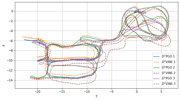
(a)

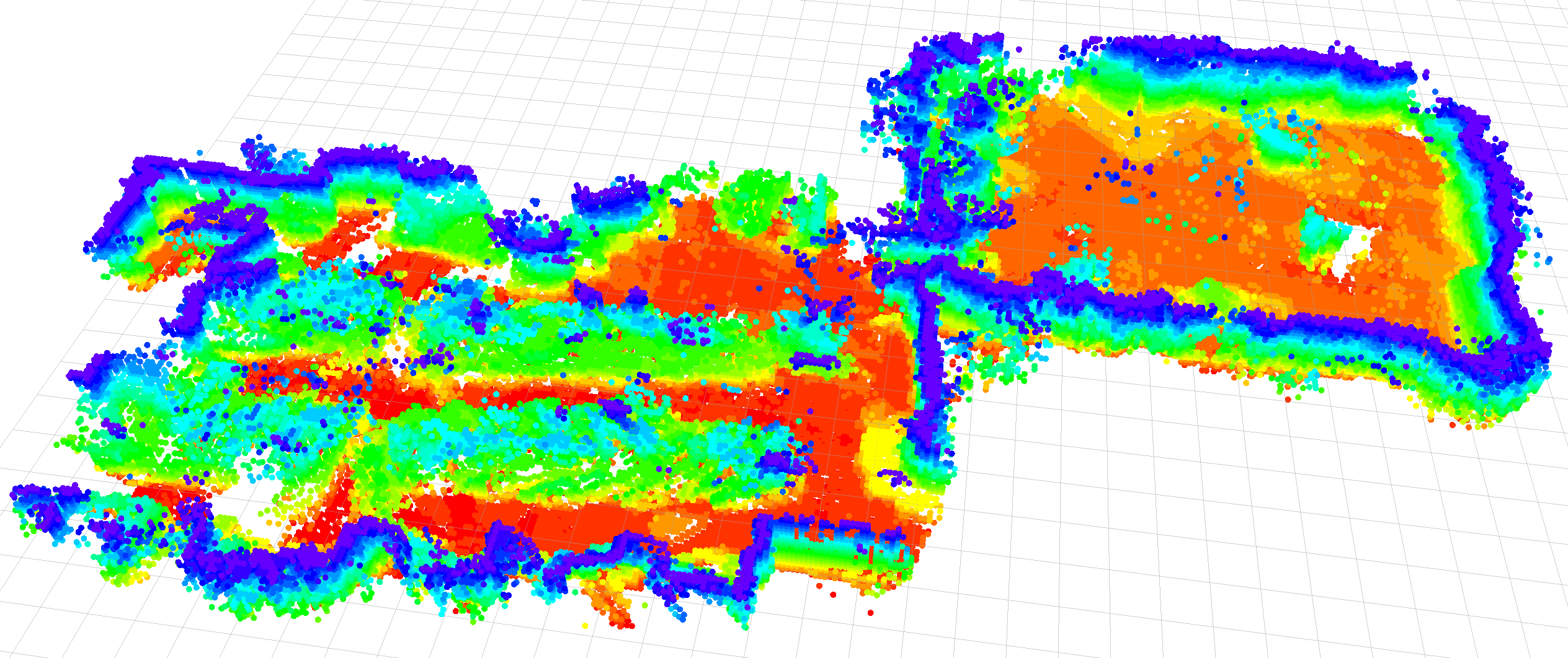
(b)

Figure 1: The demonstration of $D^{2}$SLAM on the HKUST RI dataset. a) The estimated trajectories of $D^{2}$VINS and $D^{2}$PGO of a three drone scenario. b) The dense map generated by $D^{2}$SLAM using TSDF reconstruction, only the surface voxels from TSDF are shown.

As a summary, at close distances, aerial swarm need high precision relative localization, while for longer distances, high precision relative positioning is not necessary (and difficult to achieve) and global consistency of state estimation is more important. Beyond the relative localization, among all these task, the high accuracy ego-motion estimation is essential for maintain stable flight.

In addition to the requirements given by the tasks, the CSLAM algorithms are also limited by the communication conditions. The common modes of mutual communication of robot swarm include centralized communication (for example, using a Wireless Local Area Networks) and communication using wireless ad hoc networks. The former is commonly found in laboratory environments. However, in real-world environments, robot swarm, especially aerial swarm with high mobility, need to work in a variety of complex environments where simple centralized communication is difficult to guarantee. A more practical approach is to use wireless ad hoc networks [1], where neighboring robots form a mesh network, which communication ability is limited by occlusion, communication distance, interference, etc. These networks have better communication conditions when UAVs are close to each other, but have limited communication bandwidth and stability at longer distances.

Moreover, compuation architecture of CSLAM may be difference. Broadly speaking, there are two major architectures of SLAM technology for robot swarms, centralized and decentralized. Centralized CSLAM computes information on a ground-station server, which makes it dependent on a stable network connection, while decentralized CSLAM is suitable for a wider range of situations. A well-designed decentralized approach does not depend on a stable network homology. Compared to decentralized (but redundant) CSLAM approaches, e.g. [1], distributed CSLAM has advantages of a reduced (but not costless) compuation overhead per drone, and better privacy performance: only partial information needs to be broadcast [4]. The biggest advantage of distributed SLAM is that it opens up the possibility of scaling CSLAM to large-scale swarm.

Based on the realistic requirements and communication conditions as well as the SWaP limitations of autonomous UAVs, we propose a novel CSLAM system, $D^{2}$SLAM, a decentralized and distributed visual-inertial SLAM system. $D^{2}$SLAM is designed as a highly flexible sparse SLAM system. The state estimation of $D^{2}$SLAM is a combination of two parts, near-field state estimation and far-field state estimation for aerial swarm. Here we have borrowed the terms from electromagnetism. In this paper, near-field state estimation is defined as estimating high precision real-time local state (ego-motion estimation. e.g., VIO) and high precision real-time relative state between UAVs when UAVs’ onboard sensor has field-of-view (FoV) overlap (near-field-of-view), UAVs are with good communication (near for wireless communication). Far-field state estimation is defined as estimating trajectories with global consistency when UAVs are far from each other or in non-line-of-sight (far-field-of-view), UAVs have only limited communication (far for wireless communication). The combination of these two state estimations covers well the state estimation problems we summarized above that aerial swarm need to face.

The module to achieve near-field estimation in $D^{2}$SLAM is named as $D^{2}$VINS (decentralized and distributed visual-inertial navigation system), which is a collaborative VIO system for multi-robot using sparse features. Similar to typical single-robot VIO systems (e.g., VINS-Mono [10]), $D^{2}$VINS maintain local map with sliding window, and graph-based optimization is adopted for state estimation.

Due to the general limitation of visual SLAM, one concern is that we can only get the highly accurate real-time relative state with $D^{2}$VINS if the sensor’s FoV has overlapped in a short period, even when UAVs are very close to each other, i.e., the near-field-of-view constraint. Fortunately, the omnidirectional vision system has been shown to be exceptionally effective for aerial swarm to solve the FoV issue [1]. In this paper, we also employ an improved omnidirectional visual frontend to overcome the near-field-of-view constrain. When $D^{2}$VINS works with omnidirectional cameras, the near-field-of-view is relaxed, i.e., $D^{2}$VINS will not limited by the UAVs’s yaw angle, it can be performed as long as UAVs are in line-of-sight, with common features in environments and good communication.

Nevertheless, the commerical stereo camera, e.g., Intel Realsense D435i, has been widely adopted by the state-of-the-art aerial swarm [11, 9], so they are also supported by $D^{2}$SLAM. Another advantage of a stereo camera system over a quad camera system is that it requires lower computational power and is suitable for UAVs with limited computing resources. However, when using these cameras, it is necessary to carefully set the yaw of the UAV to get the best relative state estimation accuracy, but this is out of the scope of this paper.

The core of far-field estimation is $D^{2}$PGO (decentralized and distributed pose graph optimization). $D^{2}$PGO is designed to provide global consistent state estimation, providing relative localization and global localization information even when the UAV is far away from each other or out of line of sight using pose graph optimization. Unlike $D^{2}$VINS, which only works under good communication conditions, $D^{2}$PGO is designed to work even under bad communication conditions. Therefore, we developed an asynchronous distributed pose graph optimization algorithm based on ARock.

Our near-field and far-field estimation are not independent of each other. $D^{2}$VINS and the multi-UAV loop-edge detection module together provide relative measurements (loop-edge) to $D^{2}$PGO, while $D^{2}$PGO provides initialization information to $D^{2}$VINS when the two UAVs meet. This far-to-near process can also be understood as coarse-to-fine localization.

Finally, although the core of $D^{2}$SLAM is state estimation with sparse SLAM, it can easily be extended to dense mapping. We have experimentally demonstrated dense mapping using $D^{2}$SLAM in combination with RGB-D cameras.

The main contributions of this paper are as follows:

• We propose a novel decentralized and distributed SLAM system, $D^{2}$SLAM. $D^{2}$SLAM is able to estimate the ego-motion state with high accuracy and also the relative state with high accuracy when the UAVs are close to each other, while estimating the trajectories with global consistency when the UAVs are far away from each other or not in line of sight.

• We propose a distributed visual inertial state estimator based on ADMM for multi-robot.

• We propose an ARock-based multi-robot asynchronous distributed pose graph optimization algorithm.

• The proposed $D^{2}$SLAM is tested on an aerial swarming platform by evaluating datasets and performing real experiments. The code and our custom datasets will be open source .

II Related Works

II-A Distributed SLAM techniques

This subsection discusses a series of fundamental techniques applicable to distributed SLAM, including distributed pose graph optimization, and distributed bundle adjustment.

II-A1 Distributed Pose Graph Optimization

PGO[12, 13], derived from the factor graph[14], is one of the fundamental techniques for simultaneous localization and mapping (SLAM) and is generally used for re-localization[10, 15] and dense mapping[16]. When researchers turned their attention to multi-robot collaboration, the PGO approach was naturally introduced in CSLAM as well[17, 18, 19]. Early attempts at PGO in CSLAM were accomplished by solving the pose graph problem using a centralized server[19]. However, centralized PGO suffers from scalability and communication issues in swarm robot systems. The first distributed SLAM approach, DDF-SAM, was proposed by Cunningham et al.[17]. It uses a constrained factor graph, as does its improved version DDF-SAM2[18]. However, both methods keep a neighborhood graph on each agent and optimize it on each agent, which wastes computational resources and lacks scalability.

Real progress on DPGO started with the Distributed Gauss-Seidel (DGS) approach proposed by Choudhary et al.[4]. In this method, the PGO problem is first transformed into two linear problems and then solved in a distributed manner using the Gauss-Seidel method[20]. The problem with this method is that it converges unfavorably at high noise levels and requires a synchronous operation. Later, the ASAPP method, based on distributed gradient descent, was proposed by Tian et al.[21]. It can be seen as a distributed and asynchronous version of Riemann gradient descent[22]. The highlight of that work is that it was the first to take communication into account and deliver an asynchronous DPGO approach. The subsequent work of Tian et al.[23] introduces the DC2-PGO method using the Distributed Riemann-Staircase method, which is a certifiably correct DPGO method. The above DPGO methods are currently used in several practical SLAM systems, including DOOR-SLAM[3], which utilizes DGS, and Kimera-multi[24, 2], which uses ASAPP and DC2-PGO.

II-A2 Distributed Bundle Adjustment

Bundle adjustment (BA) [25] is the basic technique in structure-from-motion (SfM) and sparse SLAM. Recently, distributed bundle adjustment problems have been developed in the SfM community [26, 27]. A Eriksson et al. proposed a distributed bundle adjustment approach by using a consensus-based distributed optimization framework [26]. This method splits a large number of camera pose into several disjoint sets and uses proximal splitting methods to build a distributed optimization solution form (also equivalent to the Alternating Direction Method of Multipliers (ADMM) method). The disadvantage of the [26] method is that all landmark information has to be exchanged among agents at each iteration of the optimization, which induces a huge communication overhead for the SFM problem. An improvement of this approach was proposed by Zhang et al.[27], in which they used a camera consensus approach, splitting landmarks into disjoint sets to build distributed optimization problems. In each iteration of the distributed optimization, only the camera pose information needs to be exchanged, and this approach is shown to have better convergence performance and much smaller communication bandwidth usage compared to [26].

However, considering the difference between the SLAM problem and SfM, these methods are not directly used. In this paper, we follow the idea of [27] and divide the landmarks into disjoint sets to build the ADMM problem, thus solving the collaborative VIO problem in a distributed manner.

In addition, [28, 29, 30] perform distributed bundle adjustment using Multi-State Constraint Kalman Filter (MSCKF). The disadvantage of the filter-based method compared to the optimization method is that the measurement can only be linearized once, so it causes a loss of accuracy.

Another distributed collaborative VIO approach is [31], which uses a loosely coupled method to fuse VIO with relative measurements. ARock [32], an asynchronous distributed optimization algorithm, is used to solve the multi-robot UWB visual fusion problem in the second stage. However, their method only considers the two-robot case and needs more flexibility.

II-B Current CSLAM systems

In this section, we summarize some existing CSLAM systems, starting with distributed SLAM methods using DPGO, including [3, 2]. Thanks to PGO, these methods have good global consistency and distributed features, but higher relative localization accuracy cannot be achieved.

[28, 29, 30, 31] use BA on landmarks for multi-camera state estimation. However, global consistency is lacking in these works.

These previously described methods use only ground features. In addition, there are some methods that use relative measurements such as UWB ranging or visual detection for relative state estimation. For example, [33, 34, 35] use UWB-odometry fusion for relative state estimation, but global consistency is lacking in these works. To scale up the UWB-odometry fusion, ARock is used for the backend optimization of the state estimation in [35]. [36] adds UWB anchor to UWB-odometry fusion to achieve global consistency, but this introduces a dependence on ground infrastructure. [1] uses a map-based localization approach to achieve global consistency. However, one problem with UWB systems is that they are susceptible to obscuration and radio interference. This makes them work with insufficient accuracy in real environments.

In addition, [33, 1, 37] introduce visual detection for relative localization, however, this makes the system limited by pre-trained detection models and makes it difficult to work when the UAVs are far apart.

In comparison to these existing systems, our work has not only global consistency, but also high relative localization at close range; in addition, our distributed architecture allows swarm scale-up. Unlike some studies [28, 29, 7, 11] that use the ground truth pose to initialize the robot pose in a global frame, which reduces the flexibility of the system, we allow the reference system and sparse map of different robots to be merged at runtime in $D^{2}$SLAM for better system flexibility.

III Preminilary

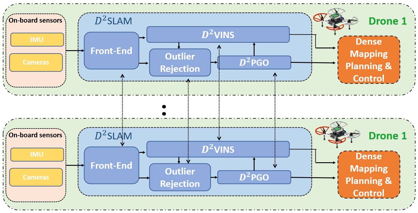
Figure 2: The architecture of $D^{2}$SLAM. The $D^{2}$SLAM is independently running on each UAV. The data will be first processed by front-end and then sent to back-end for state estimation. Results can be utilized for dense mapping, planning and control.

This paper continues the symbol system of our previous paper [1], which is not repeated here. In this paper, we assume the aerial swarm contains of $N$ UAVs, and each UAV has a unique ID $i\in\{1,2,\cdots,N\}$. If not specifically stated, these UAVs pick the initial position of the drone $k$ to establish the global reference system of the swarm. See Sect. IV-C for details on how to establish the reference system uniformly among the UAVs.

III-A State Estimation Problem of CSLAM on aerial swarm

State estimation is the core of CSLAM. For an aerial swarm that contains a maximum of $n$ homogeneous drones, the state estimation problem can be represented as follows. For every drone $k\in\mathcal{D}$, estimate the 6-DOF pose $\tensor*[^{v_{k}}]{\mathbf{T}}{{}_{i}^{t}}$ for every drone $i\in\mathcal{D}^{k}_{a}$ at time $t$ in drone $k$’s local frame, where $\mathcal{D}^{k}_{a}$ is the set of the drones has communication with drone $k$. The state estimation problem for drone $k$ can be split into two parts:

1. Estimating the ego-motion state of drone $k$ in a local frame, i.e., $\tensor*[]{\mathbf{\hat{T}}}{{}_{k}^{t}}$.

2. Estimating the state of any other arbitrary drone $i$, i.e., $\tensor*[^{v_{k}}]{\mathbf{\hat{T}}}{{}_{i}^{t}}$.

In SLAM research[38, 39], global consistency of state estimation represents that the estimate results are drift-free, e.g., the $\tensor*[^{v_{k}}]{\mathbf{\hat{T}}}{{}_{i}^{t}}$ do not drift along with the robot move.

III-B Decentralized vs Distributed

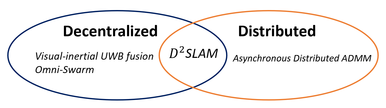
Figure 3: Visual-inertial UWB fusion [33] and Omni-Swarm [1] are decentralized, and asynchronous Distributed ADMM [40] is distributed. $D^{2}$SLAM is both decentralized and distributed.

Although decentralized and distributed are often conflated, we argue that their meanings differ. Decentralized emphasize that algorithms running on multiple nodes have no central node presence. Distributed algorithms [41] emphasize that computation (or other resources, such as storage) is distributed across multiple nodes and non-redundant computation. However, decentralized algorithms have the chance to have a large amount of redundant computation, and distributed algorithms may have a single central node.

We demonstrate the relationship between decentralization and distribution in Fig. 3. Omni-swarm [33] is decentralized but not distributed: it does not have a unique centralized node, but its optimization backend is redundant among swarm, which results in a waste of computational resources. At the same time, Asynchronous Distributed ADMM [40] uses a single master and multiple worker structures, which distributes the computation to run on multiple nodes but still requires a central node. The final goal of this paper is the proposal of a distributed and decentralized ($D^{2}$) CSLAM algorithm: $D^{2}$SLAM. It can effectively avoid the failures caused by the loss of a single node, it is more robust to the loss of communication, and it ensures that the swarm has enough autonomy to split into several sub-swarms or to form a new large swarm. Simultaneously, it can better utilize the computational resources carried by each drone.

IV System Overview

IV-A $D^{2}$SLAM System Architecture

The architecture of $D^{2}$SLAM is shown in Fig. 2. The frontend and state estimation of $D^{2}$SLAM are performed on each UAV independently. For $D^{2}$SLAM on each UAV, the visual input is first processed by the front-end for key frame extraction, sparse feature tracking, and loop closure detection, and these results are sent to the back-end for collaborative visual odometry (near-field state estimation) and pose graph optimization (far-field state estimation). $D^{2}$VINS and $D^{2}$PGO are used for near-field state estimation and far-field state estimation. Finally, the estimated result is sent to dense map building, planning, and control.

IV-B Communication Modes

We designed two communication modes for $D^{2}$SLAM to work in different situations: compact and greedy. In the compact mode, we minimize the communication overhead by: sending compact descriptors and performing distributed loop closure detection (Sect. V-E), and only sending information for near-field state estimation when drones are close to each other (Sect. V-D). In greedy mode, each drone shares all its information as much as possible, which is suitable for good network conditions but causes communication overhead.

IV-C Multi-robot Map Merging

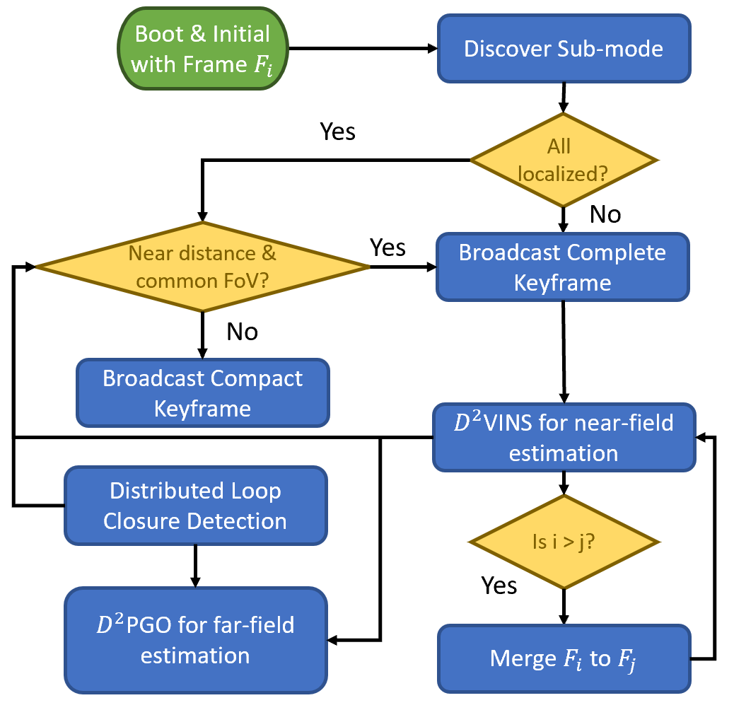
(a)

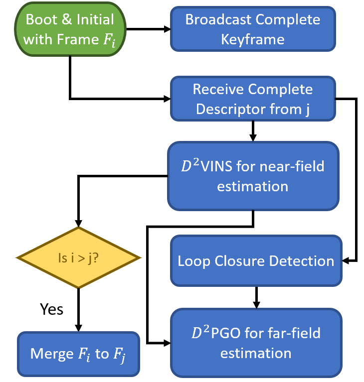
(b)

Figure 4: Flow charts of multi-robot state initialized and map merging. a) Map-merging procedure in compact mode, saving more communication; b) Map-merging in greedy mode, suitable for scenarios where communication bandwidth is not constrained.

In $D^{2}$SLAM, robots share the same reference system once they successfully establish relative state estimation. Each robot establishs a local reference frame $\mathbf{F}_{i}$ with the start position as the origin at boot time, where $i$ is the ID of the drone. As this drone meets other robots or travels across the same place visited by another drone $j$, this drone will generate relative measurements to another drone, so we perform inter-drone map merging based on the relative measurements. The map-merge process in $D^{2}$SLAM is simply a merging of coordinate systems between drones and does not involve sharing landmarks between them, i.e., each robot keeps it own sparse map. $D^{2}$SLAM on both drones select the smaller reference frame ID of the encountered UAV as the new reference system. We convert the sliding window, prior (Sect. VI-D) in $D^{2}$VINS and the keyframe pose (Sect. VII) in $D^{2}$PGO of the larger id UAV to the new reference system based on their relative measurements.

In the greedy communication mode, map-merging is directly performed by $D^{2}$VINS, as shown in Fig. 4(b). However, under the compact communication mode, the map-merging procedure is more complex, as shown in Fig. 4(a). In this mode, a drone will remain in the discover sub-mode if it detects that any other drone in the swarm has not yet been localized. In the discover sub-mode, $D^{2}$SLAM will function similar to the greedy mode until all drones in the swarm have been merged into a single coordinate system. Once map-merging is complete, subsequent state estimation will no longer require the above process.

IV-D Operating Conditions of $D^{2}$SLAM

$D^{2}$SLAM is designed as a very flexible SLAM system. Specifically, it degrades to independent stand-alone SLAM or VIO when it receives environment limitations or communication restrictions. It is proved that aerial swarm still guarantee stable flight and even perform formation flight for a short period with only standalone VIO [8]. In the following, we will discuss these limitations in detail.

IV-D1 Communication

Communication is a crucial component of collaborative SLAM. This paper focuses on UAV collaboration that involves communication between the drones. When communication is lost, $D^{2}$SLAM will degenerate into a single-robot SLAM system. On the other hand, near-field state estimation requires a larger amount of data exchange and real-time performance, so a good and low-latency network environment is needed. In contrast, far-field state estimation has lower requirements for communication bandwidth and latency, so it can be performed in a more relaxed network environment.

IV-D2 Environments

In open environments lacking environmental features, such as grass or rough walls, performing feature matching for relative localization and loop closure detection can be challenging. This difficulty is inherent in the basic characteristics of sparse visual SLAM. In such cases, to ensure flight safety, we have designed our system to degrade to VIO.

IV-D3 Field of View

Accuate relative localization is only possible when there is an FoV overlap and enough common features available. Alignment of UAVs’ yaw angle is necessary for FoV-limited cameras, but it no longer limits when using omnidirectional cameras. Nevertheless, accuate relative localization still requires that the UAV is in line of sight. Thanks to the local accuracy of $D^{2}$VINS, the loss of a few tens of seconds of common feature does not bring significant loss of relative state estimation. We argue that accuate relative localization is no longer necessary when the UAV is not in the line of sight for a long period or is far away from each others so that no valid common features are available.

V Front-end

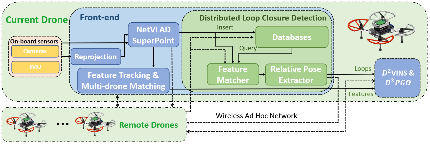
Figure 5: The front-end of $D^{2}$SLAM. The visual data is first processed by reprojection, next send to extract global descriptor and features, then send to feature tracking, multi-drone feature matching and loop closure detection. The final results will be fuse in the back-end.

$D^{2}$SLAM provides a flexible and efficient front-end for visual inputs, the front-end accepts multiple typle of camera configuration, including omnidirectional camera, stereo cameras. As shown in the Fig. 5, our front-end consists of several parts: 1) pre-processing the fisheye image for omnidirectional cameras; 2) general pre-processing to extrack landmarks and global descriptors; 3) feature tracking on local drone; 4) multi-drone sparse feature matching; 5) distributed loop closure detection.

V-A Fisheye images preprocessing

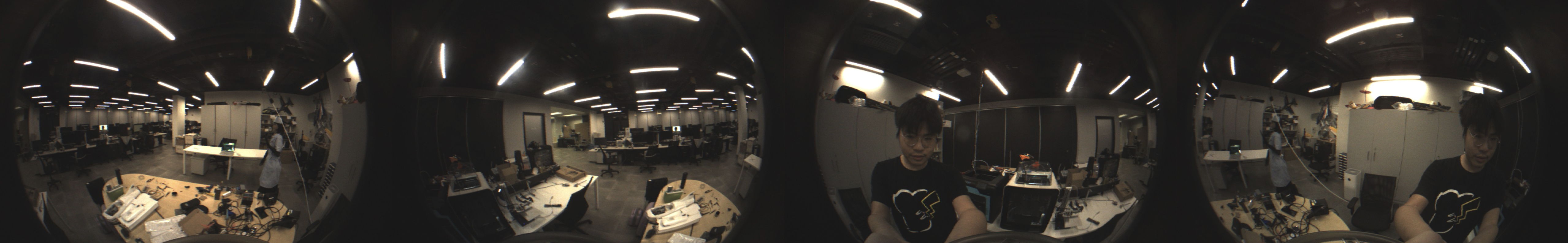
(a)

(b)

Figure 6: A demonstration of fisheye images: (a) raw fisheye images (b) reprojected fisheye images and feature tracking. The blue points are SuperPoint features and the orange points are LK features. The green arrows are the inter-frame movements of these features.

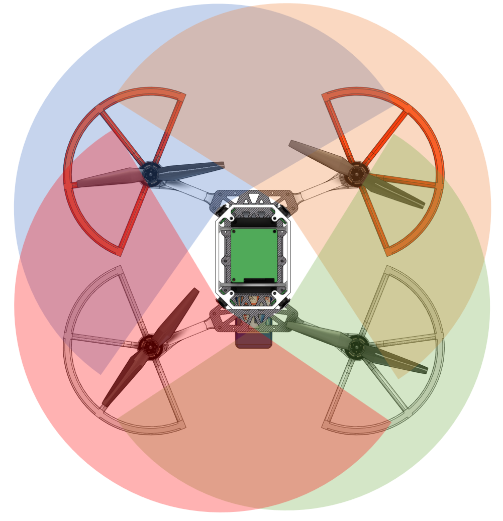
Figure 7: A demonstration of the configuration of quad fisheye cameras. The transparent areas are the FoV of each camera. Our cameras have a lateral field of view (FOV) of approximately 200 degrees, with an overlap of 110 degrees between two neighboring cameras.

In this paper, we use a quad fisheye camera system as omnidirectional camera, as shown in the Fig. 7. Compared to the dual fisheye camera system [1, 42], it uses the cameras’ FoV more effectively and generates higher quality depths. Due to these advantanges, this configuration is also adopted in SLAM research [43] and some advance product in UAV industry (e.g. DJI Mavic 3).

The fisheye camera captures images with a significant distortion, which makes it difficult to apply existing vision techniques directly, a example of the raw fisheye images is shown in the Fig. 6(a). Inspired by [44], we first reproject these images into cylindrical projection, as shown in Fig. 6(b), and then perform subsequent processing. As proved by [44], directly apply of CNNs trained using public datasets on these reprojected images deliver good results.

V-B General pre-processing

We use MobileNetVLAD [45] to build a global descriptor for each camera view. We use SuperPoint [46] to extract landmarks, PCA is also adopted for reduce the dimension of the descriptors. These techniques have been verified in our previous work [1], we do not elaborate here.

V-C Sparse Feature Tracking

Currently, two types of sparse feature tracking are applied to sparse visual SLAM: 1, using the Lucas-Kanade (LK) method (VINS-Mono [10]); 2, using descriptors for matching (ORB-SLAM [47]). The LK-based approach is more robust when the environmental features are poor (e.g., grass). However, using this method for large parallax multi-view feature matching is challenging, which is essential for multi-drone feature matching and loop closure detection. The descriptor-based approaches, especially CNN-based approaches, can handle large parallax and efficiently perform multi-drone matching or loop closure detection, but it does not work well in places with poor environmental features.

In this paper, multi-drone feature matching and robustness are both critical. So we use a hybrid front-end to balance these requirements, as shown in Fig. 6(b). The maximum number of landmarks tracked by each camera view is $N_{max}$ (100-200 in partice). On each camera view, we first extract $N_{max_{sp}}$ (50-150) sparse features and their descriptors using SuperPoint [46], assuming that the number of successful extractions is $N_{sp}$. We choose the SuperPoint feature because it is more robust than the ORB feature employed in [47]. The inter-frame tracking of these landmarks is done using a kNN matcher with ratio test [48]. We then use Shi-Tomasi corner detector to extract $N_{max}-N_{sp}$ landmarks and track them with LK method. Only SuperPoint features are used for loop closure detection and multi-drone matching, and LK landmarks only contribute to the ego-motion estimation. In some feature-less environments, the system may not detect any SuperPoint features, i.e., Nsp=0, at which point the system automatically degrades to a single robot VIO. Once feature tracking is complete, we determine whether a new frame is a keyframe based on the parallax and the number of new landmarks.

After finish the per-frame tracking, we also apply multi-view feature tracking between different cameras on same UAV. It is easy to handle when using stereo input: We directly match the SuperPoint feature point and LK optical flow for the left and right cameras. For quad fisheye cameras, each fisheye camera will only have landmarks in common with the neighboring camera’s half-plane, as shown in Fig. 7. So we only perform feature matching on SuperPoint features in the corresponding half-planes and pre-panning the positions of these landmarks according to the camera’s internal and external parameters as initialization values when solving for LK optical flow.

V-D Multi-drone Sparse Feature Matching

When a keyframe arrives, we first search the sliding window for the most recent keyframe that matches it. Two keyframes are considered to match when their global descriptors have a inner product greater than a threshold $\tau_{mg}$ (default is 0.8). If the search is successful, we perform kNN feature matching with ratio test on the Superpoint features of these two keyframes to establish the correspondence between the features. The successfully matched features are considered to belong to the same landmark and sent to the backend for near-field state estimation.

In compact communication mode, to save communication bandwidth, we only broadcast the complete keyframe information, including SuperPoint features and the global descriptors of each camera view, to other drones in the swarm when the following conditions are met:

• Robot is in discover sub-mode.

• Existing other UAVs are predicted to be in close range based on the existing state estimation results (within 3 or 5 m in an indoor environment).

V-E Distributed Loop Closure Detection

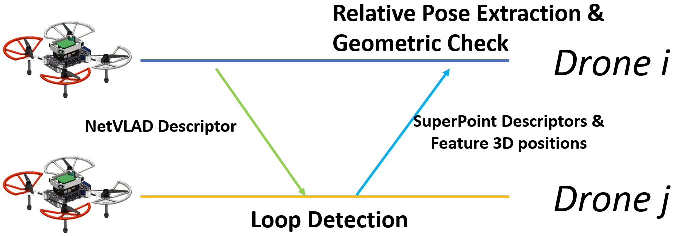
Figure 8: A demonstration of distributed loop closure detection. Drones transmit compact keyframes containing the global descriptor (NetVLAD) to the swarm. Upon receiving this information, drone j performs loop closure detection. If the match is successful, the drone sends out a complete keyframe with landmark information to be used by drone i for final relative pose extraction.

Similiar to [1], we use Faiss for whole image searching, kNN for feature matching, PnP for relative pose extraction, and outlier rejection. The loop edge is then sent to the backend for pose graph optimization. Nevertheless, distributed loop closure detection method [3, 2] is adopted in $D^{2}$SLAM’s compact communication mode to reduce the required communication bandwidth, as shown in Fig. 8.

In relative pose extraction, when using quad fisheye as input, we need to solve a multi-camera PnP problem for relative pose extraction and geometry verification. In practice, we use the UPnP RANSAC algorithm [49] for pose estimation initial and outlier rejection and then use the inlier result to solve a bundle adjustment problem for multi-camera PnP to obtain a more accurate pose. The UPnP RANSAC algorithm and the following bundle adjustment refinement in $D^{2}$SLAM is from OpenGV [50].

VI Near-field state estimation: $D^{2}$VINS

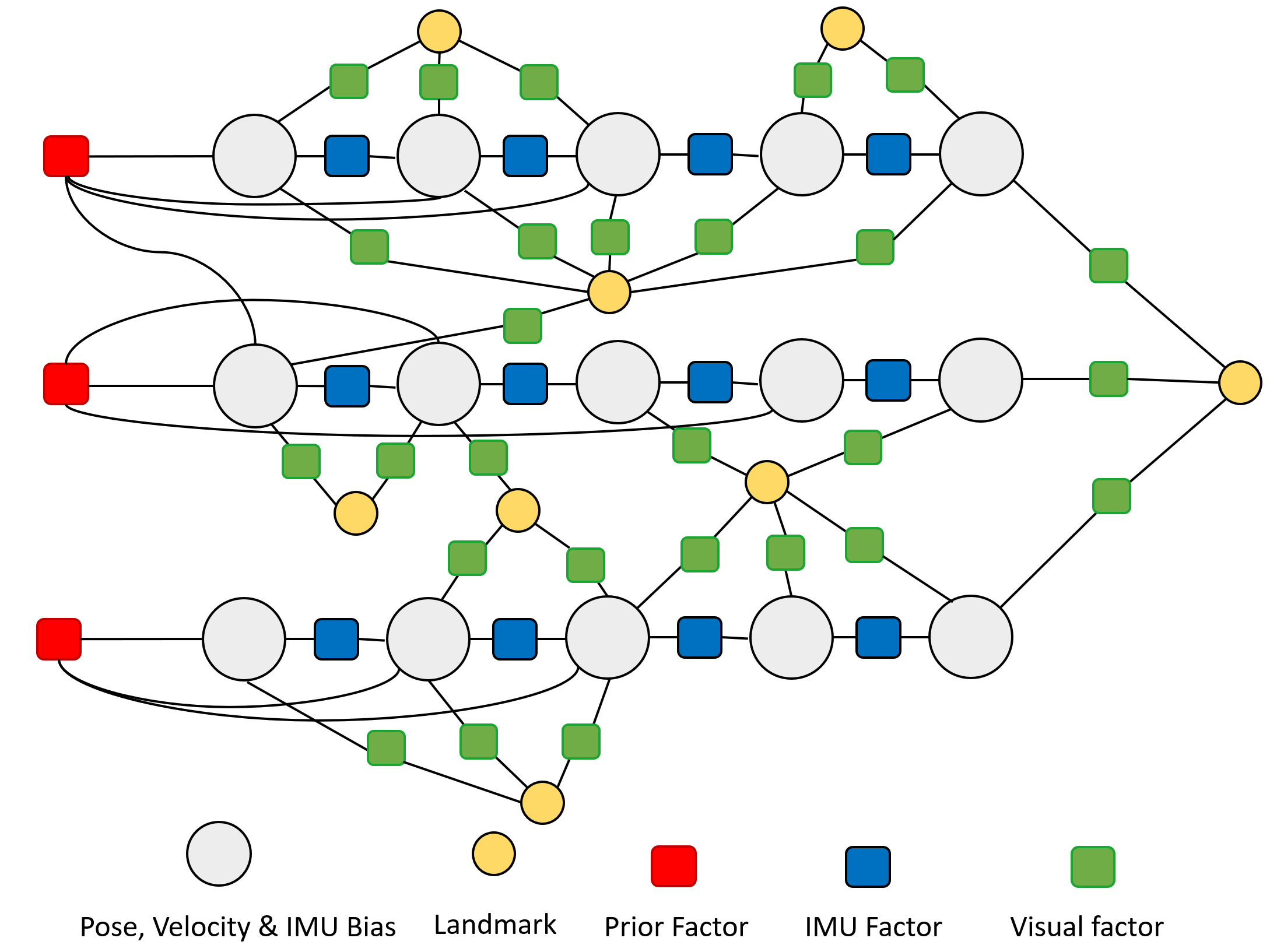
Figure 9: A demonstration of the factor graph of $D^{2}$VINS. The states in the sliding window, including pose, velocity, and IMU bias are linked together by factors including IMU factor, visual factor, and prior factor.

VI-A Problem formulation

In order to conduct near-field state estimator for $D^{2}$SLAM, we propose $D^{2}$VINS, a collaborative visual-inertial-odometer estimator. $D^{2}$VINS is designed to real-time estimate accuacte 6-DoF odometry of self drone and nearby drones which satifies the previous stated conditions. $D^{2}$VINS uses a graph optimization framework with sliding window [10]. The state estimation problem for $D^{2}$VINS can be represented using a factor graph [14], as shown in Fig. 9. We estimate the states in the sliding window by solving the maximum a posteriori (MAP) inferece of this factor graph using the distributed non-linear-least-square optimization. The state of the collaborative visual-inertial-odometry problem is define as

$$\mathcal{X}=\Big{[} {}^{v_{k}}\mathbf{\tilde{T}}_{0}^{t_{0}},^{v_{k}}\mathbf{\tilde{T}}_{0}^{t_{1}},\cdots^{v_{k}}\mathbf{\tilde{T}}_{0}^{t_{m-1}},\mathbf{b}_{0}^{t_{0}},\mathbf{b}_{0}^{t_{1}},\cdots\mathbf{b}_{0}^{t_{m-1}},$$ (1)

$$\cdots\ ^{v_{k}}\mathbf{\tilde{T}}_{1}^{t_{0}},\ ^{v_{k}}\mathbf{\tilde{T}}_{1}^{t_{1}},\cdots^{v_{k}}\mathbf{\tilde{T}}_{n-1}^{t_{m-1}},\mathbf{b}_{1}^{t_{0}},\mathbf{b}_{1}^{t_{1}},\cdots\ \mathbf{b}_{n-1}^{t_{m-1}},$$

$$l_{0},l_{1},l_{2},\cdots l_{L}\Big{]}^{T},$$

where $\tensor*[^{v_{k}}]{\mathbf{\tilde{T}}}{{}_{i}^{t_{j}}}$ is the estimated pose of UAV $i$ at time $t_{j}$ in the local frame of UAV $k$, $m$ is the length of the sliding window and $n$ is the number of the drones in the swarm, $\mathbf{b}_{i}^{t_{j}}=[\tensor*[^{v_{k}}]{\mathbf{v}}{{}_{i}^{t_{j}}},b_{a}^{t_{j}},b_{g}^{t_{j}}]$ is the velocity, acceleration bias and angular velocity bias of the IMU of UAV $i$ at time $t_{j}$, $l_{j}$ is the state of landmark $p$ and $L$ is the total number of the landmark. In this paper, we use the inverse depth parametrization [51] for landmarks, i.e. $l$ is the inverse depth from the keyframe that landmark $l_{j}$ attached to anbd the landmark $l_{j}$. For convenience, we denote the set of all poses in $\mathcal{X}$ as $\mathcal{T}$. The optimization problem for collaborative visual-inertial-odometry is formulated as,

$$\min_{\mathcal{X}}\Bigg{\{}\left\|\mathbf{r}_{p}-\mathbf{H}_{p}\mathcal{X}\right\|^{2}+ \sum_{k\in\mathcal{B}}{\left\|r_{\mathcal{B}}(\tilde{z}_{b_{k}}^{b_{k+1}},\mathcal{X})\right\|_{\Sigma_{\mathcal{B}}}}+$$ (2)

$$\sum_{k\in\mathcal{L}}{\rho\left(\left\|r_{\mathcal{L}}(\tilde{z}_{l_{k}},\mathcal{X})\right\|_{\Sigma_{\mathcal{L}}}\right)}\Bigg{\}},$$

$$s.t.\ \mathbf{P}_{i}\in\mathbf{SE}(3),\ \forall\mathbf{P}_{i}\in\mathcal{T}$$

where $\rho(\cdot)$ is the Huber norm [52], $\left\|(\cdot)\right\|_{\Sigma}$ is the Mahalanobis norm, $\mathcal{B}$ is the set of IMU factors, $\mathbf{r}_{\mathcal{B}}$ is the residual of the IMU measurement factor, $\mathcal{L}$ is the set of visual measurements, and $\mathbf{r}_{\mathcal{L}}$ is the visual measurement residual, $\mathbf{r}_{\mathcal{B}}$ and $\mathbf{r}_{\mathcal{L}}$ are define in [10] and well known to the community; $\left\|\mathbf{r}_{p}-\mathbf{H}_{p}\mathcal{X}\right\|^{2}$ is the prior factor generated from previous marginalization, which will be detailed in Sect. VI-D.

VI-B Distributed Optimization of Collaborative visual-inertial-odometry problem

VI-B1 ADMM method for decentralized and distributed optimization

The target of decentralized and distributed optimization is to solve the problem,

$$\sum_{i=1}^{n} f_{i}(\mathbf{x}_{i}),$$ (3)

$$s.t.\ \mathbf{x}_{i}=\mathbf{z},$$

using decentralized (and distributed) ADMM method [53, 27], where $\mathbf{x}_{i}$ is the local state for agent $i$ and $z$ is the global state, the problem Eq. (4) can be solved by iteratively perform the following update on each agent $i$,

$$\mathbf{x}_{i}^{t+1} =argmin_{\mathbf{x}_{i}}{\left\{f_{i}(\mathbf{x}_{i})+\frac{\rho}{2}\|\mathbf{x}_{i}-(\mathbf{z}^{t}-\mathbf{u}^{t})\|^{2}\right\}}$$ (4)

$$\mathbf{z}^{t+1} =\frac{1}{n}\sum_{i=1}^{N}\mathbf{x}_{i}^{t+1}$$ (5)

$$\mathbf{u}_{i}^{t+1} =\mathbf{u}_{i}^{t}+\mathbf{x}_{i}^{t+1}-\mathbf{z}^{t},$$ (6)

e.g. each agent $i$ solves the a new optimization problem Eq. (4) in each iteration and updates its estimate states optimization problem by averaging the results obtained by other agents.

VI-B2 Distributed optimization for $D^{2}$VINS

Rewriten Eq. (2) to the form of decentralized optimization (3), we have,

$$\min_{\mathcal{X}_{i}} \sum_{i=1}^{N}f_{cvio_{i}}(\mathcal{X}_{i})$$ (7)

$$f_{cvio_{i}}(\mathcal{X}_{i})=\left\|\mathbf{r}_{p_{i}}-\mathbf{H}_{p_{i}}\mathcal{X}_{i}\right\|^{2}+\sum_{k\in\mathcal{B}}{\left\|r_{\mathcal{B}}(\tilde{z}_{b_{k}}^{b_{k+1}},\mathcal{X}_{i})\right\|_{\Sigma_{\mathcal{B}}}}$$

$$+\sum_{k\in\mathcal{L}}{\rho\left(\left\|r_{\mathcal{L}}(\tilde{z}_{l_{k}},\mathcal{X}_{i})\right\|_{\Sigma_{\mathcal{L}}}\right)}$$

$$s.t.\ \mathcal{X}_{i}=\mathbf{E}_{i}\mathcal{X},$$

$$s.t.\ \mathbf{P}_{j}\in\mathbf{SE}(3),\ \forall\mathbf{P}_{j}\in\mathcal{T}_{i}$$

where $\mathcal{X}_{i}$ is the local state on agent $i$, which will be detailed introduced in Sect. VI-B3, $\mathbf{E}_{i}$ project the global state $\mathcal{X}$ to local state $\mathcal{X}_{i}$, $f_{cvio_{i}}(\mathcal{X}_{i})$ is the subproblem of the global optimization problem Eq. (2) on agent $i$. Follow Eq. (4)-(6), the iteration update of solving collaborative VIO problem (7) is,

$$\mathcal{X}_{i}^{t+1}= \operatorname*{arg\,min}_{\mathcal{X}_{i}}f_{cvio_{i}}(\mathcal{X}_{i})+h(\mathcal{X}_{i})$$

$$s.t.\ \mathbf{P}_{i}\in\mathbf{SE}(3),\ \forall\mathbf{P}_{i}\in\mathcal{T}_{i}$$ (8)

$$h(\mathcal{X}_{i}) =\frac{1}{2}\sum_{\mathbf{P}_{j}\in\mathcal{T}_{i}}{\|\log((\mathbf{P}^{t}_{j})^{-1}\mathbf{P}^{k}_{j})+\tilde{\mathbf{P}^{k}_{j}}^{t}\|_{\Sigma_{\rho_{T}}}}$$ (9)

$$+\rho_{\mathcal{L}}\sum_{l_{i}\in\mathcal{L}_{i}}{\|l_{i}-l_{i}^{t}\|}$$

$$\mathbf{P}_{j}^{t+1}= \frac{1}{n_{i}}\sum_{j=1}^{n_{i}}(\mathbf{P}_{j}^{k})^{t+1},\ \forall\mathbf{P}_{j}\in\mathcal{T}_{i}$$ (10)

$$(\mathbf{\tilde{P}}_{j}^{k})^{t+1}= (\mathbf{\tilde{P}}_{j}^{k})^{t}+\log((\mathbf{P}_{j}^{t+1})^{-1}(\mathbf{P}_{j}^{k})^{t}),\ \forall\mathbf{P}_{j}\in\mathcal{T}_{i},$$ (11)

where $\mathcal{X}_{i}^{t}$ is the estimate local state of agent $i$ in the $t$-th iteration, $\mathcal{T}_{i}$ is the set of the poses in $\mathcal{X}_{i}$, $\mathbf{P}_{j}$ the $j$-th pose in $\mathcal{T}_{i}$, $\mathcal{L}_{i}$ is the set of the landmarks partitioned to drone $i$ for solving, $\mathcal{B}_{i}$ is the set of the IMU factors of drone $i$, the detailed of the $\mathcal{X}_{i}^{t+1}$, $\mathcal{T}_{i}$ and $\mathcal{L}_{i}$ will be introduced later in Sect. VI-B3, $\log(\cdot)$ is the logarithm map of the Lie group SE(3)[54], which will be detailed in Sec. VI-B4, $h(\mathcal{X}_{i})$ is the consensus item to ensure the local state $\mathcal{X}_{i}$ is consistent with the global state $\mathcal{X}$, inside $h(\mathcal{X}_{i})$, the first item $\sum_{P\in\mathcal{T}_{i}}{\|\log((P^{t}_{i})^{-1}P^{k}_{i})+\tilde{P^{k}_{i}}^{t}\|_{\Sigma_{\rho_{T}}}}$ is to ensure the poses are consistent among drones and the second item $\rho_{\mathcal{L}}\sum_{l_{i}\in\mathcal{L_{i}}}{\|l_{i}-l_{i}^{t}\|}$ is to ensure the convergence of the distributed optimization as proved in [27]. The full algorithm of the distributed optimization for collaborative VIO is shown in Alg. 1.

Input: $n$ drones, $m$ landmarks, $iter$ iterations, $\rho$ and $\rho_{T}$.

Output: $n$ drones’ local states $\mathcal{X}_{i}$.

1 Initialize $\mathcal{X}_{i}$ and $\mathcal{X}$, $\mathcal{T}_{i}$, $\mathcal{L}_{i}$.

2 for $t=1$ to $iter$ do

3       Solve the local optimization problem (8) with $\mathcal{X}_{i}$

4       Broadcast the poses $\mathcal{T}_{i}$ in local state $\mathcal{X}_{i}$ to all drones

5       Update $\mathcal{X}_{i}$ with by averaging poses among swarm with Eq. (10).

6       Update the states for auxaliry variables $\{\mathbf{\tilde{P}}_{j}^{k}...\}$ using Eq. (11).

7      

Algorithm 1 Distributed optimization for Collaborative VIO on drone $i$

VI-B3 Problem Splitting

As we discussed in Sect. II-A2, a key concern in optimization with ADMM is how the problem and state are partitioned. In $D^{2}$VINS, we divide the landmarks $\mathcal{L}$ into disjoint sets $\{\mathcal{L}_{1},\mathcal{L}_{2},\cdots\mathcal{L}_{N}\}$ and use this to partition the problem and state, where the set of the landmarks partitioned to drone $i$ is denoted as $\mathcal{L}_{i}$. The landmark partition policy will be discussed in Sect. VI-C. And we define the set of poses which have observe landmarks in $\mathcal{L}_{i}$ is $\mathcal{T}_{i}$. So $\mathcal{X}_{i}$ is define as,

$$\mathcal{X}_{i}=\left[\mathcal{T}_{i},\mathcal{L}_{i},\mathbf{b}_{i}^{t_{0}},\mathbf{b}_{i}^{t_{1}}\cdots\mathbf{b}_{i}^{t_{m-1}}\right]^{T},$$ (12)

where $\mathbf{b}_{i}^{t_{0}},\mathbf{b}_{i}^{t_{1}}\cdots\mathbf{b}_{i}^{t_{m-1}}k$ are the state of the velocity and IMU bias of drone $i$, they are only essential for local optimization. Due to the presence of the hybrid tracking feature method (Sect. V-C), $\mathcal{X}_{i}$ necessarily contains all i’s pose in $\mathcal{X}$. This ensures that once all remote drone are disconnected, $D^{2}$VINS can still estimate the ego-motion, i.e., degrade to a single-robot VIO.

VI-B4 Optimization on Manifold

One key problem in SLAM is the optimization on the manifold. In Alg. 1, Problem (8) is solve by Riemannian trust region (RTR) method [22] to ensure the pose state is on $\mathbf{SE}(3)$ group, i.e., $\mathbf{P}_{i}\in\mathbf{SE}(3),\ \forall\mathbf{P}_{i}\in\mathcal{T}_{i}$. In addition, the auxiliary states $\{\mathbf{\tilde{P}}_{j}^{k}...\}$ are defined on $\mathfrak{se}(3)$. We use the logarithm map [54] to transform the error $(\mathbf{P}_{j}^{t+1})^{-1}(\mathbf{P}_{j}^{k})^{t}$ defined on $\mathbf{SE}(3)$ into $\mathfrak{se}(3)$. The quaternion averaging in Eq. (10) is solved by quaternion averaging algorithm [55], which is well known in the aerospace field.

VI-B5 Convergence Analysis

Due to the complexity of the problem, existing graph-based VIO researchers [10, 56, 24] rarely mention the convergence of optimization methods. Instead, these VIO algorithms emphasize the use of good initialization to guarantee the convergence of the algorithm. Therefore, we also discuss only the convergence of the Alg. 1 in the case of good initialization, which well be shown in Appendix -A.

VI-C Landmark Management

The $D^{2}$VINS algorithm partitions landmarks in $\mathcal{L}$ based on the drone that first detected them. In addition to landmark partitioning, it is important to set appropriate bounds on the system size to achieve real-time performance goals and maintain sufficient measurements for observability in extreme conditions. Finally, dropping outlier measurements can improve the system’s robustness and reduce the risk of false matches.

The above requirements of partitioning can be formulated as follows, for agent $k$,

$$\max_{\mathcal{L}_{k}\subseteq\mathcal{L}} (w_{l}m_{l}(\mathcal{L}_{k})+w_{r}m_{r}(\mathcal{L}_{k})-w_{o}o(\mathcal{L}_{k})),$$ (13)

$$\max_{\mathcal{L}_{k}\subseteq\mathcal{L}} \min_{j,t}m(\mathcal{L}_{k},\mathcal{K}_{j}^{t})$$ (14)

s. t. $$|\mathcal{L}_{k}|\leq\tau_{l}$$ (15)

$$m_{l}(\mathcal{L}_{k})+m_{r}(\mathcal{L}_{k})\leq\tau_{m}$$ (16)

$$\mathcal{L}_{k}\subseteq\mathcal{LD}_{k},$$ (17)

where landmarks may have multiple measurements and $m_{l}(\mathcal{L}_{k})$ and $m_{r}(\mathcal{L}_{k})$ represent the number of measurements to landmarks in $\mathcal{L}_{k}$ from local keyframes (keyframes generated by drone $k$ itself) and remote keyframes, respectively, $o(\mathcal{L}_{k})$ is the number of outlier measurements to landmarks in $\mathcal{L}_{k}$. The weights $w_{l}$, $w_{r}$ and $w_{o}$ determine the importance of these measurements in the objective function. The size of $\mathcal{L}_{k}$ is limited by $\tau_{l}$ and the maximum measurements is limited by $\tau_{m}$. $\mathcal{L}_{k}\subseteq\mathcal{LD}_{k}$ is to ensures that $\mathcal{L}$ is partitioned into disjoint sets, where $\mathcal{LD}_{k}$ is the subset of $\mathcal{L}$ containing the landmarks discovered by drone $k$ first. $\mathcal{K}_{j}^{t}$ is a frame in the sliding window and $\max_{\mathcal{L}_{k}}\min_{j,t}m(\mathcal{L}_{k},\mathcal{K}_{j}^{t})$ seeks to maximize the lower bound of the number of measurements from every single keyframe. Problem 13 is a multi-objective optimization problem, which can also been seen as an extended coverage problem. We address this problem by proposing a novel multi-robot landmark selection (MLS) algorithm, as shown in Alg. 2.

Input: Current drone $k$, available landmarks $\mathcal{L}$, set of available keyframes $\{\mathcal{F}\}$, a dictionary $\mathcal{O}$ representing the observed landmarks of each frame, with the relationship $\mathcal{O}[\mathcal{F}]\rightarrow\mathcal{L}_{f}$.

Output: Set of selected landmarks $\mathcal{L}_{k}$

1 $\mathcal{N}_{l}\leftarrow\emptyset$

2 $\mathcal{L}_{k}\leftarrow\emptyset$

3 $\mathcal{O}_{a}\leftarrow\mathcal{O}$

4 foreach $\mathcal{F}\in\{\mathcal{F}\}$  do

5       $\mathcal{N}_{l}[\mathcal{F}]\leftarrow 0$

6while True do

7       if $empty(\mathcal{N}_{l}$) then

8             break

9      $\mathcal{F}\leftarrow\operatorname*{arg\,min}_{\mathcal{F}\in\{\mathcal{F}\}}{\mathcal{N}_{l}[\mathcal{F}]}$

10       if $empty(\mathcal{O}_{a}[\mathcal{F}])$ then

11             $\mathcal{N}_{l}\leftarrow\mathcal{N}_{l}\setminus\{\mathcal{F}\}$

12             continue

13      $l\leftarrow\operatorname*{arg\,max}_{l\in\mathcal{O}_{a}[\mathcal{F}]}cost(k,\mathcal{F})$

14       foreach $track\in l.tracks$  do

15             $\mathcal{N}_{l}[track.\mathcal{F}]\leftarrow\mathcal{N}_{l}[track.\mathcal{F}]+1$

16            

17      $\mathcal{L}_{k}\leftarrow\mathcal{L}_{k}\cup\{l\}$

18       foreach $\mathcal{F}\in\{\mathcal{F}\}$  do

19             $\mathcal{O}_{a}[\mathcal{F}]\leftarrow\mathcal{O}_{a}[\mathcal{F}]\setminus\{l\}$

20      if $|\mathcal{L}_{k}|>\tau_{l}$ or $m_{l}(\mathcal{L}_{k})+m_{r}(\mathcal{L}_{k})>\tau_{m}$ then

21             break

22      

23

Algorithm 2 Multi-robot Landmark Selection

In Alg. 2, we defined a cost function to approximate the objective function in Eq. (13),

$$cost(l,\mathcal{F})=\begin{cases}w_{l}m_{l}(l)+w_{r}m_{r}(l)-w_{o}o(l)&\text{if }l\in\mathcal{LD}_{k}\\ -1&\text{otherwise},\end{cases}$$ (18)

where $m_{l}(l),m_{r}(l)$ are the number of measurements to landmark $l$ from local keyframes and remote keyframes, respectively, and $o(l)$ is the number of outlier measurements to landmark $l$.

To select the landmarks, the algorithm first initializes the dictionary $\mathcal{N}_{l}$ to record the current number of measurements of each landmark, and the dictionary $\mathcal{O}_{a}$ to record the landmarks observed by each frame that have not been selected yet. In each iteration of the algorithm, the keyframe in the sliding window with the least number of measurements is found (line 2. This step is to approximate Eq. (14). A landmark $l$ observed by that keyframe is selected that maximizes Eq. (18). The algorithm then updates the dictionary $\mathcal{N}_{l}$ by incrementing the number of measurements of $l$ for each keyframe of the measurement track in $l.tracks$. The selected landmark $l$ is added to $\mathcal{L}_{k}$, and the dictionary $\mathcal{O}_{a}$ is updated to remove the selected landmark from the observed landmarks of each keyframe. The algorithm continues until either the number of selected landmarks exceeds a predefined threshold $\tau_{l}$, selected measurements achieve $\tau_{m}$ or there are no available measurements in any keyframe. The selected landmarks are returned in $\mathcal{L}_{k}$.

Alg. 2 is an approximation of Eq. (13), but when there are fewer common landmarks among robots, Eq. (17) may not hold, so landmarks can be reused on different robots. This increases computation and decreases accuracy, but it is necessary for the robustness of $D^{2}$VINS. Our experiments showed that in fewer measurements per frame case, the system becomes unstable and even diverges, so a tradeoff is made in Alg. 2 to ensure stability.

In practice, we set $w_{l}=1,w_{r}=2$ to ensure that more feature points across robots are added and $w_{o}=2$ to avoid possible outlier. The criterion of outlier measurement is its reprojection error is too large before the optimization starts.

VI-D Sliding Window & Marginalization

$D^{2}$VINS uses a sliding window to manage keyframes, and each drone manages only its keyframes. Similar to [10], when a new frame is added, the second new frame in is discarded if it is not a keyframe, otherwise, the oldest keyframe is discarded. After the sliding window is updated, $D^{2}$VINS will push the latest sliding window information to the other drone in the swarm.

When the old keyframes are discarded, we linearize each subproblem ($f_{cvio_{i}}(\mathcal{X}_{i})$) of the problem (7) and compute a new set of priors $\{(\mathbf{r}_{p_{0}},\mathbf{H}_{p_{0}}),(\mathbf{r}_{p_{1}},\mathbf{H}_{p_{1}})\cdots(\mathbf{r}_{p_{N-1}},\mathbf{H}_{p_{N-1}})\}$ using the Schur complement by dropping the old states. This procedure is well-known as marginalization [10, 56]. In marginalization, these subproblems are treated as independent, so the marginalization process is also run distributively. Nevertheless, the problem (7) is solved with states averaged over different drones (Eq. 10), so the marginalization among drones are consistent, i.e., on different drones, the states are linearized with the same or very close linearization points.

VI-E Initialization

The initialization of $D^{2}$VINS is divided into two parts, the initialization of the local keyframe and the initialization of the remote drone. $D^{2}$VINS uses stereo or multi-camera, so we directly use triangulation to initialize the location of landmarks has measurements with enough baseline (0.05cm in practical) from multi-cameras or from motion, and also use IMU prediction to initialize the subsequent keyframe pose from local drone. After initialization, we add priors to the unobservable part ($x,y,z,yaw$) of the first frame to increase stability. For the case of multiple drones, we use PnP RANSAC (or gPnP) to initialize the pose of the remote keyframe when the coordinate system reference of the remote drone is different from the local drone.

VI-F Implementation

In $D^{2}$SLAM, Problem (8) is solved using Ceres-solver [57] with Dogleg strategy [58] and dense Schur solver as the linear solver. In this implementation, we use Local Parameterization from ceres to add the on manifold constraints of the poses. This combination can be consider as RTR method [22].

Due to Eq. (10), Alg. 1 is a synchronous method, which requires the UAV to wait for the results of other UAVs at each iteration. The synchronization method causes a decrease in efficiency when the communication environment is poor. Fortunately, we have found in practice that relaxing the condition of Eq. (10), i.e., averaging the state of the other drones received most recently each time without waiting, also yields results close to those of the synchronous method. We refer to this method as asynchronous $D^{2}$VINS. A comparison of asynchronous versus synchronous $D^{2}$VINS will be shown in IX-B.

VII Far-field state estimation: $D^{2}$PGO

Complete far-field estimation includes the estimation of global consistent trajectories ($D^{2}$PGO) and real-time global consistent odometries. We use pose graph [59] for modeling the trajectories estimation problem: keyframes of the trajectory are represented as nodes on the graph, and different keyframes are connected by edges representing relative poses. The pose graph can be expressed as a factor graph, and assuming that the measurement is Gaussian distributed, thus is the well-known pose graph optimization problem [14]:

$D^{2}$PGO uses two-stage optimization to decentralize and distribute solve the pose graph optimization problem for multiple drones. The pose graph optimization problem is,

$$\min_{\mathbf{x}_{i}} \sum_{(i_{t_{0}},j_{t_{1}})\in\mathcal{E}}\left\|{}^{v_{k}}\mathbf{\hat{p}}_{j}^{t_{1}}-{}^{v_{k}}\mathbf{\hat{p}}_{i}^{t_{0}}-{}^{v_{k}}\mathbf{\hat{R}}_{i}^{t_{0}}{\mathbf{z}_{\mathbf{p}}}_{i\rightarrow j}^{t_{0}\rightarrow t_{1}}\right\|^{2}_{\Sigma_{t}}$$ (19)

$$+\left\|{}^{v_{k}}\mathbf{\hat{R}}_{j}^{t_{1}}-{}^{v_{k}}\mathbf{\hat{R}}_{i}^{t_{0}}{\mathbf{z}_{\mathbf{R}}}_{i\rightarrow j}^{t_{0}\rightarrow t_{1}}\right\|^{2}_{\Sigma_{R}},$$

$$s.t.\ {}^{v_{k}}\mathbf{\hat{R}}_{i}^{t}\in SO(3),$$

where $\mathcal{E}$ is the set of all edge, including loop closure edge (generated by loop closure detection) and ego-motion edge (generated by $D^{2}$VINS), ${}^{v_{k}}\mathbf{R}_{i}^{t}$ is the rotation part of ${}^{v_{k}}\mathbf{\hat{T}}_{i}^{t}$, and ${}^{v_{k}}\mathbf{p}_{i}^{t}$ is the translation part of ${}^{v_{k}}\mathbf{\hat{T}}_{i}^{t}$, $\mathbf{x}$ is the full state of the pose graph:

$$\mathcal{X}=\Big{[} {}^{v_{k}}\mathbf{\hat{T}}_{0}^{t_{0}},^{v_{k}}\mathbf{\hat{T}}_{0}^{t_{1}},\cdots^{v_{k}}\mathbf{\hat{T}}_{0}^{t_{M-1}},\cdots\ ^{v_{k}}\mathbf{\hat{T}}_{1}^{t_{0}},$$ (20)

$${}^{v_{k}}\mathbf{\hat{T}}_{1}^{t_{1}},\cdots^{v_{k}}\mathbf{\hat{T}}_{N-1}^{t_{M-1}}\Big{]},$$

where $N$ is the number of drones, $M$ is the number of keyframes of each drone.

$D^{2}$PGO uses two-stage approach to solve the pose graph optimization problem (19) decentralize and distributedly. Rewriting the pose graph optimization problem (19) in distributed manner (4), we have:

$$\min_{\mathbf{x}_{i}}\sum_{i=0}^{N-1}f_{pgo_{i}}(\mathbf{x}_{i})$$ (21)

$$f_{pgo_{i}}(\mathbf{x}_{i}) =\sum_{(i_{t_{0}},j_{t_{1}})\in\mathcal{E}^{i}}\left\|{}^{v_{k}}\mathbf{\hat{p}}_{j}^{t_{1}}-{}^{v_{k}}\mathbf{\hat{p}}_{i}^{t_{0}}-{}^{v_{k}}\mathbf{\hat{R}}_{i}^{t_{0}}{\mathbf{z}_{\mathbf{p}}}_{i\rightarrow j}^{t_{0}\rightarrow t_{1}}\right\|^{2}_{\Sigma_{p}}$$

$$+ \left\|{}^{v_{k}}\mathbf{\hat{R}}_{j}^{t_{1}}-{}^{v_{k}}\mathbf{\hat{R}}_{i}^{t_{0}}{\mathbf{z}_{\mathbf{R}}}_{i\rightarrow j}^{t_{0}\rightarrow t_{1}}\right\|^{2}_{\Sigma_{R}},$$

$$s.t.\ {}^{v_{k}}\mathbf{\hat{R}}_{i}^{t}=\mathbf{E}^{\mathbf{R}}_{i_{t}}\mathbf{z},{}^{v_{k}}\mathbf{\hat{p}}_{i}^{t}=\mathbf{E}^{p}_{i_{t}}\mathbf{z},{}^{v_{k}}\mathbf{R}_{i}^{t}\in SO(3),$$

where $x_{i}$ is the state of the drone $i$, $\mathcal{E}^{i}$ is the set of edges of the drone $i$.

In the first stage of $D^{2}$PGO, we use the initialize the rotation of the pose graph to avoid local minima. In the second stage, we refine the optimization of the pose graph. In addition to pose graph optimization, we also adopt a outlier rejection module to reject outliers in the pose graph optimization problem (19).

Finally, we combine the pose graph optimization result with the VIO result to obtain the global consistent trajectory of each drone:

$$\tensor*[^{v_{k}}]{\mathbf{\hat{T}}}{{}_{i}^{t_{1}}}=\tensor*[^{v_{k}}]{\mathbf{\hat{T}}}{{}_{i}^{t}}(\tensor*[]{\mathbf{\tilde{T}}}{{}_{i}^{t}})^{-1}\tensor*[]{\mathbf{\tilde{T}}}{{}_{i}^{t_{1}}},$$ (22)

where $\tensor*[^{v_{k}}]{\mathbf{\hat{T}}}{{}_{i}^{t}}$ is the pose of the latest keyframe of UAV $i$ in $D^{2}$PGO and $\tensor*[]{\mathbf{\tilde{T}}}{{}_{i}^{t}}$ is the odometry estimation with $D^{2}$VINS of this keyframe, $\tensor*[]{\mathbf{\tilde{T}}}{{}_{i}^{t_{1}}}$ is the real-time odometry estimation with $D^{2}$VINS.

VII-A ARock for Distributed Optimization

We use ARock [32], an asynchronous distribution optimization algorithm to solve the PGO. ARock uses follow iteration update to solve the distributed optimization problem (3), the [32]:

$$\mathbf{\hat{x}}_{i}^{t}= \operatorname*{arg\,min}_{\mathbf{x}_{i}}f_{i}(\mathbf{x_{i}})+\mathbf{x_{i}}\sum_{r\in\mathcal{R}(i)}z^{t}_{ri,r}+\frac{\gamma}{2}|\mathcal{R}(i)|\cdot\|\mathbf{x_{i}}\|^{2}$$ (23)

$$z^{t+1}_{ri,i}= z_{ri,i}^{t}-\eta_{k}((z^{t}_{ri,i}+z_{ri,r})/2+\gamma\mathbf{\hat{x}}_{i}^{t})\ \forall r\in\mathcal{R}(i),$$ (24)

where $\mathcal{R}(i)$ is the set of neighbors of agent $i$, $(\cdot)^{t}$ means state of $t$-th iteration, $\eta_{k}$ and $\gamma$ are two parameters. $z_{ij,i},z_{ij,j}$ are the dual variables for for agent $i$ and it neighbor $j$, and will be update by agent $i$ and $j$ respectively. We rewriting the update rule replacing the dual variables $z_{ri,i}^{t},z_{ri,r}^{t}$ with $y_{ij,i}=-z_{ij,i}/\gamma,y_{ij,j}=-z_{ij,j}/\gamma$,

$$\mathbf{\hat{x}}_{i}^{t}= \operatorname*{arg\,min}_{\mathbf{x}_{i}}f_{i}(\mathbf{x_{i}})+\sum_{r\in\mathcal{R}(i)}\frac{\gamma}{2}\|\mathbf{x_{i}}-y^{t}_{ri,r}\|^{2}$$ (25)

$$y^{t+1}_{ir,i}= y_{ir,i}^{t}-\eta_{k}((y^{t}_{ir,i}+y_{ir,r})/2-\mathbf{\hat{x}}_{i}^{t})\ \forall r\in\mathcal{R}(i)$$ (26)

Alg. 3 shows the full algorithm of ARock for decentralized optimization. Unlike the Alg. 1 we used earlier, ARock is an asynchronous algorithm. We only need to use the latest received dual variables from remote without running the equations synchronously, as in Eq. (25)-(26), which means that ARock is more insensitive to communication delays. Moreover, Alg. 3 is proved to be linear convergence [32].

Input: $n$ drones, $m$ landmarks, $iter$ iterations.

1 Initialize $y_{ij,i}^{0},y_{ij,j}^{0}$ for all $i,j$ to $0$.

2 for $t=1$ to $iter$ do

3       Solve the local optimization problem (25)

4       Update the dual states $y^{t}_{ir,i}$ with Eq. (26).

5       Broadcast the dual state $y^{t}_{ir,i}$ to all drones

6       if Convergence then

7             Break

8      

Algorithm 3 ARock for distributed optimization

VII-B Asynchronous Distributed Rotation Initialization

The nonlinearities in the pose graph problem come from rotations. When rotations are properly initialized, the pose graph optimization problem approaches a linear least sqaure problem and is easily solved. The rotation initialization technique has been proved effective in avoiding local minima of the pose graph optimization [60]. The target of rotation initialization is find the solution or a approximate solution for the rotation part of problem (19), which is also known as the rotation averaging problem [61]:

$$\min_{\mathbf{x}_{i}} \sum_{(i_{t_{0}},j_{t_{1}})\in\mathcal{E}^{i}}{\left\|{}^{v_{k}}\mathbf{\hat{R}}_{j}^{t_{1}}-{}^{v_{k}}\mathbf{\hat{R}}_{i}^{t_{0}}{\mathbf{z}_{\mathbf{R}}}_{i\rightarrow j}^{t_{0}\rightarrow t_{1}}\right\|^{2}_{\Sigma_{R}}}$$ (27)

$$s.t.\ {}^{v_{k}}\mathbf{\hat{R}}_{i}^{t}\in SO(3).$$

An efficient and powerful algorithm for solving this problem is Chordal relaxation [62]. In this algorithm, we first solve the problem by relaxing the $\mathbf{SO}(3)$ constrain of (27):

$$\min_{\mathbf{x}_{i}}\sum_{(i_{t_{0}},j_{t_{1}})\in\mathcal{E}} {\left\|{}^{v_{k}}\mathbf{\overline{R}}_{j}^{t_{1}}-{}^{v_{k}}\mathbf{\overline{R}}_{i}^{t_{0}}{\mathbf{z}_{\mathbf{R}}}_{i\rightarrow j}^{t_{0}\rightarrow t_{1}}\right\|^{2}_{\Sigma_{R}}}$$ (28)

$$+\sum_{{\overline{R}}_{i}^{t}\in\mathcal{R}_{i}}{\|{}^{v_{k}}(\mathbf{\overline{R}}_{i}^{t})_{3}-\mathbf{v}_{i}\|}_{\Sigma_{g}},$$

where $\mathcal{R}_{i}$ is the set of all rotations in $\mathbf{x}_{i}$, $\mathbf{\overline{R}}_{i}^{t}$ is the a 3x3 matrix of drone $i$ at time $t$, $\|{}^{v_{k}}(\overline{\hat{R}}_{i}^{t})_{3}-\mathbf{v}_{i}\|$ is the vertical prior, this item is added because the roll pitch angle of VIO is observable and thus can be use as a prior to enhance the initialization [60], ${}^{v_{k}}(\mathbf{\overline{R}}_{i}^{t})_{3}$ is the third row of matrix $\mathbf{\overline{R}}_{i}^{t}$, $\mathbf{v}_{i}=(\mathbf{\tilde{R}}_{i}^{t})^{T}\mathbf{g}$, $g=[0,0,1]^{T}$, $\mathbf{\tilde{R}}_{i}^{t}$ is the odometry output rotation of drone $i$ at time $t$. Problem (28) is a linear least sqaure problem which can be efficient solved by a linear solver. Then, we can recover the rotation matrix by

$${}^{v_{k}}\mathbf{\hat{R}}_{i}^{t}= argmin_{\mathbf{\hat{R}}}\|\mathbf{\hat{R}}-{}^{v_{k}}\mathbf{\overline{R}}_{i}^{t}\|^{2}_{F},$$ (29)

$$s.t.\ \hat{R}\in\mathbf{SO}(3)$$

where $\|\cdot\|_{F}$ is the Frobenius norm. Problem (29) has a closed form soluting with SVD decomposition [61]:

$${}^{v_{k}}\mathbf{\breve{R}}_{i}^{t}=\mathbf{S}diag([1,1,det(\mathbf{SV^{T}})])\mathbf{V^{T}},$$ (30)

where ${}^{v_{k}}\mathbf{\breve{R}}_{i}^{t}\in SO(3)$ is the initial result of ${}^{v_{k}}\mathbf{\hat{R}}_{i}^{t}$, $\mathbf{SDV^{T}}$ is the SVD decomposition of $\mathbf{\overline{R}}_{i}^{t}$.

In $D^{2}$PGO, Problem (28) is solved in a distributed manner, rewriting the problem as,

$$\min_{\mathbf{x}_{i}}\sum_{i=0}^{N-1} \Bigg{\{}\sum_{(i_{t_{0}},j_{t_{1}})\in\mathcal{E}_{i}}{\left\|{}^{v_{k}}\mathbf{\overline{R}}_{j}^{t_{1}}-{}^{v_{k}}\mathbf{\overline{R}}_{i}^{t_{0}}{\mathbf{z}_{\mathbf{R}}}_{i\rightarrow j}^{t_{0}\rightarrow t_{1}}\right\|^{2}_{\Sigma_{R}}}$$ (31)

$$+\sum_{{\overline{R}}_{i}^{t}\in\mathbf{x}_{i}}{\|{}^{v_{k}}(\mathbf{\overline{R}}_{i}^{t})_{3}-\mathbf{v}_{i}\|_{\Sigma_{g}}}\Bigg{\}},$$

Applying Alg. 3 to solve for problem (31) leads to the proposed asynchronous distributed rotation initialization algorithm, as shown Alg. 4. The local optimization problem (bring Eq. (31) into Eq. (25)) in Alg. 4 is a linear least square problem, which is solved efficiently by using Cholesky factorization [63]. We terminate the iterations when the change in the state being optimized is small, as shown in Alg. 31 line 4, where $(\mathbf{\overline{R}})^{t}$ is the state after $t$ iteration. Moreover, to prevent premature termination, e.g., no data was received at the beginning, we also set a minimum number of iterations.

Input: $\epsilon$ for termination, $max\_iter$ iterations, $min\_iter$ to avoid early exiting.

1 Initialize $y_{ij,i}^{0},y_{ij,j}^{0}$ for all $i,j$ to $0$.

2 for $t=1$ to $max\_iter$ do

3       Solve the local optimization problem (25) with $f_{i}$ defined from (31)

4       Update the dual states $y^{t}_{ir,i}$ with Eq. (26).

5       Broadcast the dual state $y^{t}_{ir,i}$ to neighbors

6       if $\frac{1}{|\mathcal{R}_{i}|}\sum_{\mathbf{\overline{R}}\in\mathcal{R}_{i}}{{\|(\mathbf{\overline{R}})^{t}-(\mathbf{\overline{R}})^{t-1}\|_{F}}/{\|(\mathbf{\overline{R}})^{t}\|_{F}}<\epsilon}$ and $iter>min\_iter$  then

7             break

8      

9for $\overline{R}\in\mathcal{R}_{i}$ do

10       Recover the rotation ${}^{v_{k}}\mathbf{\hat{R}}_{i}^{t}$ with Eq. (30)

11      

Algorithm 4 Asynchronous Distributed Rotation Initialization for drone $i$

1 while Not shutdown do

2       if New data received then

3             Adding new states or cost functions to optimizer.

4      Solve the local optimization problem (25) with $f_{i}$ defined from (32)

5       Update the dual states $y^{t}_{ir,i}$ with Eq. (26).

6       Broadcast the dual state $y^{t}_{ir,i}$ to neighbors

7       Recover the poses with Eq. (33)

8       Sleep for a while

Algorithm 5 Asynchronous Distributed Pose Graph Optimization for drone $i$

VII-C Asynchronous Distributed Pose Graph Optimization

After completing the initialization, we build the perturbation problem of (21) with the initialization rotation,

$$\min_{\mathbf{x}_{i}^{*}}\sum_{i=0}^{N-1}f_{pgo_{i}}(\mathbf{x}_{i}^{*})$$ (32)

$$f_{pgo_{i}}^{*}(\mathbf{x}_{i}^{*}) =\sum_{(i_{t_{0}},j_{t_{1}})\in\mathcal{E}^{i}}\big{\|}{}^{v_{k}}\mathbf{\hat{p}}_{j}^{t_{1}}-{}^{v_{k}}\mathbf{\hat{p}}_{i}^{t_{0}}-$$

$$\boxplus({}^{v_{k}}\mathbf{\breve{R}}_{i}^{t_{0}},{}^{v_{k}}\mathbf{\delta\theta}_{i}^{t}){\mathbf{z}_{\mathbf{p}}}_{i\rightarrow j}^{t_{0}\rightarrow t_{1}}\big{\|}^{2}_{\Sigma_{p}}+$$

$$\left\|\boxplus({{}^{v_{k}}\mathbf{\breve{R}}_{j}^{t_{1}}},{}^{v_{k}}{\delta\theta}_{j}^{t_{1}})-\boxplus({}^{v_{k}}\mathbf{\breve{R}}_{i}^{t_{0}},{}^{v_{k}}\mathbf{\delta\theta}_{i}^{t}){\mathbf{z}_{\mathbf{R}}}_{i\rightarrow j}^{t_{0}\rightarrow t_{1}}\right\|^{2}_{\Sigma_{R}},$$

$$s.t.\ {}^{v_{k}}\mathbf{\delta\theta}_{i}^{t}=\mathbf{E}^{\mathbf{R}}_{i_{t}}\mathbf{z}^{*},{}^{v_{k}}\mathbf{\hat{p}}_{i}^{t}=\mathbf{E}^{p}_{i_{t}}\mathbf{z}^{*},$$

where $({}^{v_{k}}\mathbf{\hat{p}}_{i}^{t_{0}},{}^{v_{k}}\mathbf{\delta\theta}_{i}^{t_{0}})$ is the perturbation state of ${}^{v_{k}}\mathbf{T}_{i}^{t_{0}}$, where ${}^{v_{k}}\mathbf{\hat{p}}_{i}^{t_{0}}$ is the position of ${}^{v_{k}}\mathbf{T}_{i}^{t_{0}}$ and ${}^{v_{k}}\mathbf{\delta\theta}_{i}^{t_{0}}\in\mathfrak{so}3$ is the perturbation state of the rotation. $x_{i}^{*}$ is the the perturbation state of $\mathbf{x}^{i}$, and $\mathbf{z}^{*}$ is the global perturbation state, $\boxplus(\mathbf{R},\mathbf{\delta\theta})=\mathbf{R}Exp(\mathbf{\delta\theta}_{i}^{t_{0}})$ retracts $\mathfrak{so}3$ vector to $\mathbf{SO}(3)$ at $\mathbf{R}$[22], where $Exp(\cdot)$ maps $\mathfrak{so}3$ to $SO(3)$ [64]. Unlike Eq (10) in [4], which also uses a two-step PGO, (32) is a nonlinear problem that avoids the accuracy problems of [4] due to linearization.

We also apply Alg. 3 to solve (32), which ensures that our algorithm is asynchronous. In addition, taken $f_{pgo_{i}}^{*}(\mathbf{x}_{i}^{*})$ into (25) result a nonlinear least sqaure problem, which can be solved with Levenberg-Marquardt algorithm [65]. Finally, we use the change in the cost of $f_{pgo_{i}}^{*}(\mathbf{x}_{i}^{*})$ to determine if it converges, and like Alg. 4, a minimum number of iterations is used to prevent premature exits. After the convergence, we recover the global pose with

$${}^{v_{k}}\mathbf{\hat{T}}_{i}^{t}{}^{v_{k}}=\begin{bmatrix}\boxplus({}^{v_{k}}\mathbf{\breve{R}}_{i}^{t_{0}},{}^{v_{k}}\mathbf{\delta\theta}_{i}^{t})&\mathbf{\hat{p}}_{i}^{t}\\ 0&1\end{bmatrix}$$ (33)

Our asynchronous distributed pose graph optimization (ARockPGO) algorithm is shown in Alg. 5. Differing from Alg. 4, throughout the operation of the UAV, we continuously iterate the ARock update at a fixed frequency (typically 1Hz) of in ARockPGO and incremently add informations to it. This is a trade-off between the convergence speed and the communication overhead.

VII-D Convergence

ARock is shown to have good convergence performance, and we believe he can converge to optimality on the first stage of a typical linear least squares problem. The results of rotation initialization prove to be effective in avoiding subsequent iterative optimization into the wrong local optimum [60], thus ensuring that $D^{2}$PGO can reach or close to the global optimum.

VII-E Outlier Rejection

Pairwise consistent measurement set maximization (PCM) [66, 3, 1] and Graduated non-convexity (GNC) [67] are currently mainstream outlier rejection methods applied to multi-robot PGO. The advantage of PCM is that it is completely decoupled from the back-end optimization, but the disadvantage is that the performance is lower when the pose graph is huge; GNC is embedded in the back-end optimization, and the advantage is that it is more efficient, but GNC is a synchronous algorithm. In $D^{2}$PGO, we use a distributed version of PCM as in [1, 3], which can avoid some of the efficiency problems of PCM at large scales, and we believe that its performance is sufficient for PGO solutions that do not require real-time.

VII-F Implementation

The first stage ensures that $D^{2}$PGO can still estimate the trajectories correctly in a highly noisy environment. In real-world experiments, we do not always need the first stage because the yaw measurement of VIO is fairly accurate.

We implemented $D^{2}$PGO using C++, where we solve the linear least sqaure of rotation initialization with Eigen[68]’s LLT algorithm. And we use the Levenberg-Marquardt algorithm from Ceres-solver [57] for the second stage.

VIII System Setup

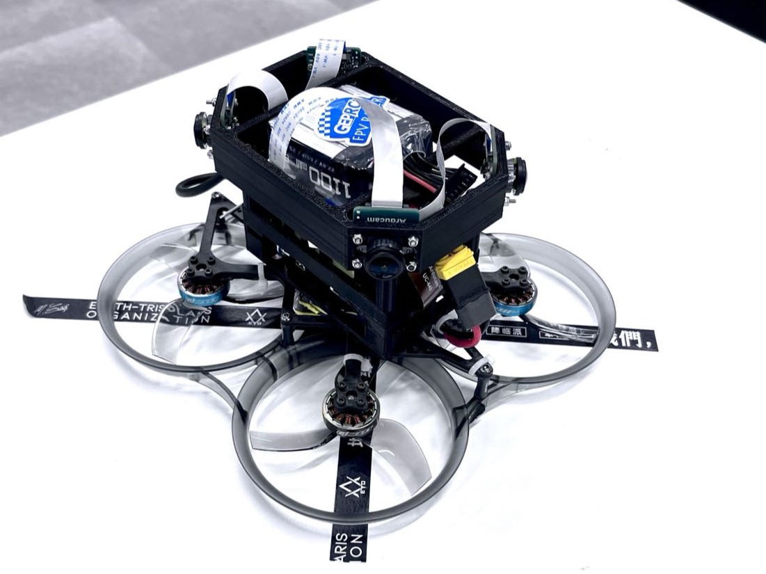
(a)

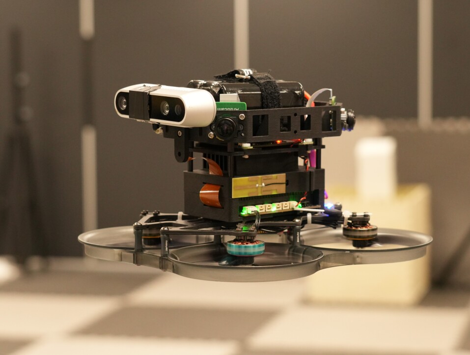
(b)

Figure 10: a) Our experiment aerial platform, which equips four fisheye cameras, an onboard computer, and an all-in-one flight controller. b) Our experiment aerial platform with an additional Intel RealSense d435i camera and 6s 18650 battery.

Our experimental aerial swarm consists of customized aerial robot platforms as shown in Fig. 10. This platform is a modified commercial 3.5-inch cinewhoop FPV drone equipped with four fisheye cameras that provide a 360-degree field of view in the horizontal direction. The onboard computer is an NVIDIA Xavier NX with a strong GPU computing power. We use a lightweight all-in-one flight controller with four integrated electronic speed controls (ESCs) and customized PX4 [69] flight control firmware to reduce the takeoff weight. This drone has a takeoff weight of about 623g when using a 22.8v 1550mah battery, and its maximum endurance is about 10 minutes, which is sufficient for testing. In addition, an Intel RealSense d435i camera can also be installed on the UAV.

We implemented $D^{2}$SLAM using C++ and used ONNX Runtime [70] for inference of the CNNs in the previous section. We enable TensorRT for acceleration and used the int8 mode of TensorRT on the onboard computer to maximize the running speed. Furthermore, we developed TaichiSLAM, a GPU-accelerated mapping module, as the mapping backend for the dense mapping experiments later on. TaichiSLAM is written in the high-performance computing language Taichi [71] and includes various algorithms, such as OctoMap[72], TSDF & ESDF [73] and submap fusion [74] for generation of global consistent map. Dense mapping algorithms are not the core part of $D^{2}$SLAM, and we will not discuss them in detail.

IX Experiments

IX-A Datasets

TABLE I: The table displays the datasets used for validation. The numbers added as suffix to the datasets correspond to the number of robots involved.

Dataset	Robot Number	Sensors	Movement	Groundtruth	Source
TUM ROOM 2-5	2 to 5	Stereo Camera IMU	HandHold	Yes	[75]
TUM Corr 2-5	2 to 5			Partial
HKUST RI 3	3	Stereo Camera Depth Camera IMU		No	Customized
Omni 2-5	2 to 5	Quad camera IMU	Flight	Yes
OmniLongNoYaw 5	5		Flight with Yaw Angle Fixed
OmniLongYaw 5	5		Flight with Yaw Angle Moving

In the evaluation presented in this section, we tested $D^{2}$SLAM using various publicly available and customized datasets. These datasets use either stereo cameras or quad cameras as input and partly used a motion capture system to capture ground truth data, as shown in Tab. I. To simulate the scenario of multiple robots operating simultaneously, we align multiple segments of data into a single multi-robot dataset.

The definition of evaluation metrics can be found in [1]. It is worth noting that, Relative Error (RE) in this paper represent the accuracy of relative state estimation among UAVs.

IX-B Evaluation of $D^{2}$VINS

We first test $D^{2}$VINS separately to verify the performance of our near-field state estimation. Here we use the greedy communication mode and operate $D^{2}$VINS independently. In our tests, we do not use any groundtruth to initialize $D^{2}$VINS. We also compare $D^{2}$VINS to the state-of-the-art visual-inertial-odometry VINS-Mono[10], we align VINS-Mono using the initial pose of ground truth to simulate the case of known UAV departure points as in [8].

TABLE II: The table shows the statistical results of $D^{2}$VINS compared to VINS-Mono [10] on TUM VI room dataset, where the ATE and RE are defined in [1]. These datasets has good common FoV at the first 30s, so we show the results individually with labeled (30s).

Dataset	Avg. Traj. Len.	Method	$ATE_{pos}$	$ATE_{rot}$	$RE_{pos}$	$RE_{rot}$
TUM ROOM 3 (30s)	18.3	$D^{2}$VINS	0.030	0.99	0.025	0.77
		$D^{2}$VINS (async)	0.035	1.63	0.025	0.74
		VINS-Mono	0.105	3.47	0.126	3.41
TUM ROOM 3	141.6	$D^{2}$VINS	0.128	2.40	0.119	2.95
		$D^{2}$VINS (async)	0.111	2.63	0.098	3.08
		VINS-Mono	0.176	2.84	0.216	3.81
TUM ROOM 4 (30s)	19.1	$D^{2}$VINS	0.057	2.20	0.020	0.74
		$D^{2}$VINS (async)	0.124	1.73	0.038	0.78
		VINS-Mono	0.108	4.01	0.113	2.76
TUM ROOM 4	100.9	$D^{2}$VINS	0.115	2.44	0.080	1.72
		$D^{2}$VINS (async)	0.105	2.18	0.082	1.85
		VINS-Mono	0.161	2.80	0.165	2.53
TUM ROOM 5 (30s)	19.2	$D^{2}$VINS	0.079	1.35	0.039	0.73
		$D^{2}$VINS (async)	0.108	4.50	0.037	0.89
		VINS-Mono	0.101	4.54	0.109	3.43
TUM ROOM 5	103.5	$D^{2}$VINS	0.090	1.85	0.073	1.57
		$D^{2}$VINS (async)	0.134	4.05	0.091	2.10
		VINS-Mono	0.176	3.03	0.176	2.80

TABLE III: The table shows the statistical results of $D^{2}$VINS compared to VINS-Mono [10] on Omni datasets. The average distance (Avg. Dis.) of the UAVs is also shown in the table. OmniLongNoYaw 5 and OmniLongYaw 5 are the long-term datasets with 5 UAVs, where drones keeping rotating yaw angle in OmniLongYaw 5.

Dataset	Avg. Traj. Len.	Avg. Dis.	Method	$ATE_{pos}$	$ATE_{rot}$	$RE_{pos}$	$RE_{rot}$
Omni 2	49.1	0.68	$D^{2}$VINS	0.068	0.74	0.035	0.14
			$D^{2}$VINS (async)	0.105	4.47	0.065	0.15
			VINS-Mono	0.237	6.60	0.271	0.52
Omni 3	48.2	0.7	$D^{2}$VINS	0.058	0.63	0.033	0.16
			$D^{2}$VINS (async)	0.059	1.21	0.037	0.14
			VINS-Mono	0.263	6.60	0.271	0.66
Omni 4	58.5	0.88	$D^{2}$VINS	0.065	0.62	0.043	0.15
			$D^{2}$VINS (async)	0.060	0.84	0.047	0.24
			VINS-Mono	0.262	4.94	0.315	0.61
Omni 5	45.4	1.03	$D^{2}$VINS	0.067	0.80	0.048	0.21
			$D^{2}$VINS (async)	0.060	1.07	0.049	0.20
			VINS-Mono	0.282	4.74	0.332	0.61
OmniLongNoYaw 5	213.7	0.48	$D^{2}$VINS	0.122	0.83	0.043	0.53
			$D^{2}$VINS (async)	0.118	0.71	0.031	0.51
			VINS-Mono	0.500	1.78	0.307	1.26
OmniLongYaw 5	237.0	0.38	$D^{2}$VINS	2.322	11.09	0.028	0.65
			$D^{2}$VINS (async)	2.752	18.32	0.027	0.72
			VINS-Mono	4.865	12.48	1.466	3.40

As shown in the Tab. II, our method demonstrates centimeter-level localization accuracy on the TUM ROOM dataset. The relative localization is very accurate (2.5cm) in the first 30s of TUM ROOM datasets, where common FoV is good in this case. Throughout the full evaluation, the dataset still demonstrates centimeter-level relative localization accuracy, similar to the best localization accuracy we showed in the state-of-the art works [33, 1], despite the absence of common FoV the vast majority of the time. This evaluation demonstrates that $D^{2}$VINS can perform highly accurate near-field state estimation even on stereo cameras, especially when the common field of view is sufficient, and the value of $D^{2}$VINS for applications on widely used stereo camera UAV platforms.

We further test $D^{2}$VINS on custom omnidirectional camera datasets; the results are shown in the Tab. III. Our method exhibits centimeter-level relative localization accuracy in all cases from 2 to 5 UAVs case. We also note the fact that the relative localization accuracy slightly decreases as the relative distance between the UAVs increases in the Tab. III. Fortunately, the need for inter-drone collision avoidance can still be met. Although $D^{2}$VINS and VINS-Mono drift away from the ground truth (large ATE in table III) in long duration flight with rotated yaw (OmniLongYaw 5) due to the nature of visual odometry, $D^{2}$VINS still maintains centimeter level relative localization accuracy in this case. This verifies the relative localization capability in long duration flight.

Overall, when common FOV presents, the relative localization accuracy of $D^{2}$VINS is better than the state-of-the-art relative localization results in [33, 1] while being accuracy on ego-motion estimation (better ATE compared to VINS-Mono). When the common FoV is unstable, then the relative localization accuracy behaves similarly to [33, 1]. Neverthelesss, our results surpass all metrics compared to VINS-Mono in Tab. II and Tab. III. This proves the superiority of our algorithm over traditional visual inertial odometry in the multi-robot scenarios. In particular, the drifts of VINS-Mono can make its relative localization accuracy poor after a long period of operation.

Furthermore, Tab. II shows the accuracy comparison of asynchronous $D^{2}$VINS ($D^{2}$VINS (async) in the table), we find that asynchronous $D^{2}$VINS performs close to that of synchronous methods. However, in some cases, the accuracy of asynchronous methods can show some instability in ATE. Considering the advantages of asynchronous methods in communication, deploying asynchronous versions in realistic environments is an acceptable tradeoff.

IX-C Evaluation of $D^{2}$PGO

TABLE IV: This table shows the comparison of $D^{2}$PGO with or without rotation initialization. Initial and final cost are shown in the table.

Dataset	Avg. Traj. Len.	Method	Initial Cost	Final Cost	Iterations	Solve Time (s)
TUM Corr 5	255.6	$D^{2}$PGO	350408.6	61.2	234.2	10.1
		$D^{2}$PGO (NoRotInit)		1920.4	238.4	10.1
OmniLongYaw 5	242.6	$D^{2}$PGO	520424.1	1366.3	37.2	20.5
		$D^{2}$PGO (NoRotInit)		41072.3	31.6	20.4
HKUST RI 3	164.5	$D^{2}$PGO	6438.5	12.1	152.0	3.0
		$D^{2}$PGO (NoRotInit)		1301.8	197.0	3.0

We present the optimization results of $D^{2}$PGO for different pose graphs generated by the front-end of $D^{2}$SLAM and $D^{2}$VINS in Table IV. In the evaluation, we add a fixed communication latency of 50ms to simulate to real-world communication delay. We compare the results of $D^{2}$PGO in optimization with and without rotation initialization. It can be observed that rotation initialization significantly helps prevent $D^{2}$PGO from entering the local optimum.

IX-D Evaluation of $D^{2}$SLAM

TABLE V: The table shows the statistical results of $D^{2}$SLAM compared to DOOR-SLAM [3] on our custom datasets. The estimated trajectories and ground truth are aligned using multiple states [76] with the first robot’s estimation.

Dataset	Method	$ATE_{pos}$	$ATE_{rot}$	$RE_{pos}$	$RE_{rot}$
OmniLongYaw 5	$D^{2}$SLAM	0.168	3.33	0.037	0.91
	DOOR-SLAM	0.149	3.47	0.085	0.72
TUM ROOM 5	$D^{2}$SLAM	0.032	0.72	0.079	1.90
	DOOR-SLAM	0.064	1.47	0.122	1.86
TUM Corr 5	$D^{2}$SLAM	0.275	3.93	0.206	1.77
	DOOR-SLAM	0.068	1.26	0.145	2.39

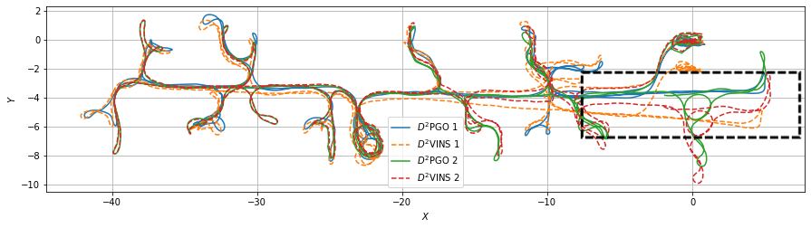
Figure 11: The figure shows the estimated trajectories of $D^{2}$SLAM on TUM Corr 2 Dataset. The TUM Corr 2 dataset is the combination of TUM VI corridor datasets {1, 2}. Two robots go through the same corridor sequentially in the black box section. The $D^{2}$VINS trajectories show significant drift in the black box section, while the $D^{2}$PGO trajectories have no significant drift, and the trajectories of the two robots are well aligned.

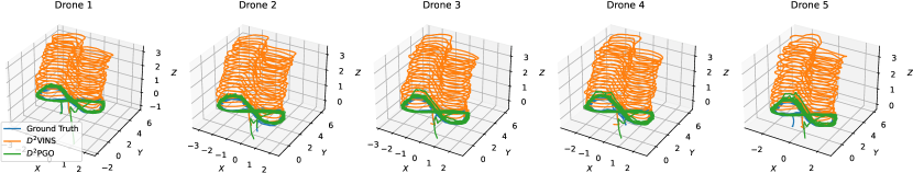
Figure 12: The images show the trajectories estimated by $D^{2}$VINS and $D^{2}$PGO in OmniLongYaw 5 datasets. Trajectories estimated by $D^{2}$VINS drift away. Will the trajectories estimated by $D^{2}$PGO follow close to the ground truth.

We futher $D^{2}$SLAM on the public and custom datasets to verify the performance of our near- and far-field state estimation. We first compare $D^{2}$SLAM with one of the state-of-the-art distributed CSLAM system DOOR-SLAM [3] on datasets with ground truth, and the result is shown in Tab. V. In the comparison, we use our custom implementation in $D^{2}$SLAM to generate PGO for DOOR-SLAM to avoid interference caused by different frontends.

In Tab. V, we can see that our method has a advantage over DOOR-SLAM in terms of relative state estimation on first two datasets. This is because DOOR-SLAM uses pose graph optimization, which is more commonly used in CSLAM, where the state estimation is loosely coupled. In terms of global consistency, the accuracy of the two methods is comparable due to their uses of similar input. One exception is that DOOR-SLAM demonstrates better accuracy on the TUM Corr dataset. The reason is that the TUM Corr dataset has only partial ground truth and there is no good yaw overlapping between drones at the end of the dataset.

We further test $D^{2}$SLAM on the TUM VI Corr 5 and HKUST RI 3 dataset to verify the global consistent on a large scale, where the real-time odometry and final pose graph estimated from the experiment is shown in Fig. 11 and Fig. 1(a).

As shown in figures, unlike results from $D^{2}$VINS drift away from the start point, trajectories estimated by $D^{2}$PGO return to the starting point. Moreover, in Fig. 11, $D^{2}$PGO well align the trajectories of the two robots in the corridor (highlighted by the black box), while $D^{2}$VINS results drift from each other because the two robots did not pass through the corridor simultaneously. These result demonstrate global consistency of $D^{2}$SLAM in the far-field case.

Fig. 1(b) shows the results of TSDF reconstruction using $D^{2}$PGO and submap fusion. There are no evident drift in the map, which also verifies the global consistency of $D^{2}$SLAM.

IX-E Scalability

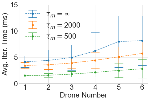
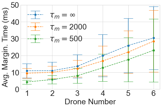
(a)

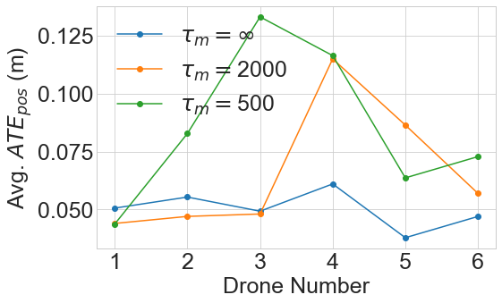
(b)

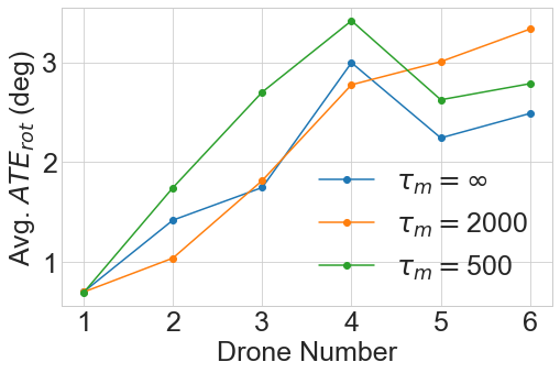
(c)

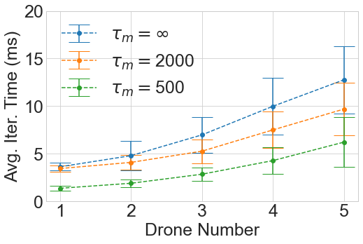
(d)

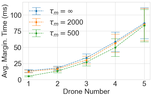
(e)

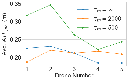
(f)

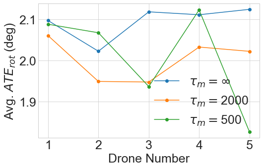
(g)

(h)

Figure 13: The average time of each iteration, marginalization time, translation error and rotation error of $D^{2}$VINS with different number of robots. $\tau_{l}=200$ in the evaluation and we compare the results with different $\tau_{m}$. a)-d) are the results of stereo camera, e)-h) are the results of quad camera.

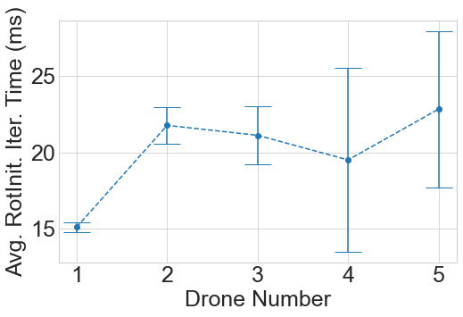
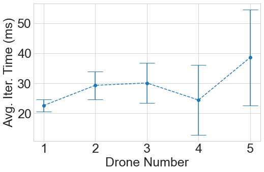
(a)

(b)

Figure 14: The average time of each iteration of $D^{2}$PGO with different number of robots. a) is the result of rotation initialization, e)-h) is the result of ARockPGO.

In this section, we discuss the scalability of the computation.

IX-E1 Front-end

The computational requirements for performing remote feature matching and loop closure detection in the front-end of $D^{2}$SLAM increase approximately linearly with the number of robots nearby. These front-end algorithms are rapid and their computational speed in real-world experiments is shown in Table VIII.

IX-E2 Back-end

The back-end situation is more complicated: In this paper we introduce distributed optimization methods to solve the graph optimization problem. In practice, however, $D^{2}$VINS uses a specially designed landmark selection algorithm MLS as a balance of computational efficiency, accuracy and robustness. This algorithm allows the number of visual measurements to be computed by $D^{2}$VINS to increase as the number of robot increases until it reaches the bound of $\tau_{m}$. This is because we set a relatively large value of $\tau_{m}$ to make $D^{2}$VINS more robust.

In Fig. 13 and Fig. 14, we demonstrate the scalability of $D^{2}$VINS and DPGO by showing how the average computation time per operation increases with the size of the swarm. As the size of the swarm increases, the size of the problem grows quadratically. However, with $D^{2}$SLAM, the computational requirement for optimization increases no more than linearly, demonstrating the effectiveness of our algorithm. Moreover, $D^{2}$SLAM allows for controlling the computational size through adjustable parameters $\tau_{m}$ and $\tau_{l}$, making it adaptable to various computational platforms. It is worth noting that reducing computational complexity through these parameters does not lead to a significant decrease in accuracy. The time taken by marginalization grows more with the number of robots, while the computation of marginalization should theoretically be similar to the iteration of one solver. This is primarily because, in the existing ceres-solver framework, the conventional practice is to convert the result of marginalization into square root form to incorporate optimization [10, 56], which we will further optimize in the future.

IX-F Communication

TABLE VI: Typical message size and broadcast frequency in $D^{2}$SLAM. $D^{2}$VINS Update and $D^{2}$PGO update are messages that are used to synchronize the optimization among swarms in $D^{2}$SLAM. $p^{k}$ is the number of poses in the drones’ sliding window. The variable $e^{k}$ is defined as the sum of dual states in ARock.

Item	Complete Keyframe (Stereo)	Complete Keyframe (Omni)	Compact Keyframe (Stereo)	Compact Keyframe (Omni)	$D^{2}$VINS Update	$D^{2}$PGO Update
Size	20.1kB	56.3kB	1.2kB	4.8kB	$0.188+0.036p^{k}$kB	$0.056+0.064e^{k}$kB
Frequency	5	5	5	5	5	1

Effective communication is a crucial factor for the success of aerial swarm work. To provide insight into this, we present the sizes and broadcast frequency of the main messages transmitted by the $D^{2}$SLAM instances running on each drone in Table VI.

For a swarm consisting of 5 drones, the maximum value of $p^{k}$ is 51, resulting in a maximum of 3.5kB of $D^{2}$VINS update per time step. The amount of $e^{k}$ depends on the map and the environment, e.g., in the TUM Corr 5 dataset, a typical value of $e^{k}$ is 1262, which corresponds to a 81kB size of each $D^{2}$PGO update.

We compared the use of greedy communication mode and compact communication mode and presented the results in Table VII. The compact mode can significantly reduce the amount of communication bandwidth needed when the UAVs spread out quickly.

TABLE VII: The total communication volume in MB of $D^{2}$SLAM in greedy mode and compact mode.

Dataset	Mode	Front-end	Back-end
			$D^{2}$VINS	$D^{2}$PGO
OmniLongYaw 5	Greedy	1546.7	75.9	2340.9
	Compact	984.2	70.8	2179.4
TUM ROOM 5	Greedy	266.4	1.6	42.0
	Compact	244.2	1.2	31.0
TUM Corr 5	Greedy	344.2	2.4	60.1
	Compact	323.0	2.9	74.1
HKUST RI 3	Greedy	231.8	10.1	13.4
	Compact	105.4	9.6	11.9

IX-G Real-world Experiments of $D^{2}$SLAM

TABLE VIII: Typical compuational time and running frequency of each module in the real-world experiment of $D^{2}$VINS.

Item	Image Preprocesing	Feature Tracking (Local)	Feature Tracking (Remote)	Optimization	Marginalization
Frequency	15 Hz	15 Hz	5 Hz	5 Hz	5 Hz
Time cost	41.7ms	2.67ms	1.64ms	56.23ms	16.88ms

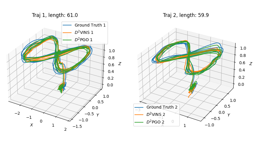
Figure 15: The images show the trajectories estimated by $D^{2}$VINS and $D^{2}$PGO in real-world experiment.

TABLE IX: The table shows the $D^{2}$SLAM accuracy for the two flight experiments. To better show global consistency, we align the estimated trajectories with ground truth by using multiple states [76]. We only use the estimated results of the first drone for alignments to avoid disturbing relative localization accuracy.

		$ATE_{pos}$		$ATE_{rot}$		$RE_{pos}$
Experiment	Avg. Traj. Len.	$D^{2}$VINS	$D^{2}$PGO	$D^{2}$VINS	$D^{2}$PGO	x	y	z	$RE_{rot}$
Drone2 NoYaw	51.0	0.103	0.090	2.24°	1.95°	0.047	0.067	0.056	3.36°
Drone2 Yaw	73.3	0.219	0.147	5.69°	4.17°	0.124	0.144	0.100	8.88°

In addition to the dataset’s validation, we tested $D^{2}$SLAM realistic environments using our UAV platforms. In real-world experiments, $D^{2}$SLAM withstood the challenges of limited computing power and communication capability and performed as expected, as shown in the Fig. 15 and Table IX.

We show data from two flights in the table, accomplished by two drones equipped with Realsense d435i and running the stereo version of $D^{2}$SLAM. In the Drone2 NoYaw experiment, both drones fix their yaw angles during flight, while in Drone2 Yaw, they rotate yaw angles follow the flight trajectory. $D^{2}$SLAM showed good global consistency in both flights: the ATE of $D^{2}$PGO was only ten centimeters for flights between 50 and 70 m long. The ATE accuracy of $D^{2}$PGO was also better than that of $D^{2}$VINS, demonstrating the importance of $D^{2}$PGO for $D^{2}$SLAM to achieve global consistency. In relative localization, $D^{2}$SLAM achieves centimeter accuracy in fixed yaw. However, in the rotating yaw experiment, $D^{2}$SLAM has less relative localization accuracy, which is caused by the limitation of stereo version $D^{2}$SLAM due to the limited FoV, as we mentioned earlier.

Table VIII shows the performance of the important algorithms of $D^{2}$SLAM when run on the onboard computer in the real-world experiments and their operating frequency. Moreover, in the real-world experiment, the communication condition was fluidity: the average communication delay is 23.89ms. We can see that $D^{2}$SLAM achieves the real-time requirement on real-world systems.

X Conclusion and Future Work

In this paper, we propose $D^{2}$SLAM, a distributed and decentralized collaborative visual-inertial SLAM system. Our experiments verify that $D^{2}$SLAM has real-time high-precision local localization capability and high-precision relative localization when the UAVs are near each other, i.e., highly accurate near-field state estimation. Globally consistent trajectories can be estimated at the same time, i.e. global consistent far-field state estimation. We believe that $D^{2}$SLAM’s flexible sensor configuration, with state estimation capabilities suitable for various missions, including self-assembly aerial swarm, cooperative transportation, inter-drone collision avoidance, and unknown environments exploration, will contribute to the development of aerial swarm research.

$D^{2}$SLAM presented in this paper still has some limitations, which we will improve in the future: 1) Despite using a distributed backend, swarm scale growth is still limited by communication capabilities, front-end computing capabilities. In the future, we will improve $D^{2}$SLAM to make it apply to enormous aerial swarms. 2) Compared to our previous work, $D^{2}$SLAM is designed as a more traditional visual SLAM work without introducing relative measurements, including UWB, mutual visual detection, etc. We believe that this allows $D^{2}$SLAM to be adapted to more situations, such as occlusions that would cause inaccurate UWB measurements; and robots that are difficult to identify accurately with visual detection. However, relative measurements is efficiency in some scenarios, and we will explore the use of relative measurements in $D^{2}$SLAM in the future.

Futhermore, we believe that $D^{2}$SLAM can be applied not only to multi-robot systems but also as a distributed visual inertial SLAM system on a single robot, e.g., deploying several nodes running $D^{2}$SLAM on a rigid UAV or ground robot for more accurate state estimation and robust in case of single node failure. Different nodes can even form distributed stereo cameras to measure the long-range environment [31]. Alternatively, $D^{2}$SLAM can be deployed on multi-rigid robots (e.g., multi-legged), and corresponding constraints can be introduced to help multi-rigid robots estimate their state and environment more accurately and provide redundancy.

-A Convergence of Distributed Collaborative VIO

Decentralized ADMM adopted by Alg. 1 was proven to have linear convergence performance on convex problems by Shi, Wei et. al. [53]. However, the bundle adjustment residual $r_{\mathcal{L}}(\hat{z}_{l_{k}},\mathcal{X}_{i})$ is not convex, and our algorithm introduces constraints on the manifold, which complicates the problem. Since RTR method compute a small step on tangent space $\mathfrak{se}(3)$ of the manifold, then retract back to the manifold $\mathbf{SE}(3)$, Update (8)-(11) are equivalent to iterating over $\mathfrak{se}(3)$ when the system is well initialized and initial pose are subtracted. We consider this simplification update of Alg. 1:

$$\mathcal{X}_{i}^{t+1}= \operatorname*{arg\,min}_{\mathcal{X}_{i}}\Bigg{\{}r_{pb}(\mathcal{V}_{i})+\sum_{k\in\mathcal{L}_{i}}{\rho\left(\left\|r_{\mathcal{L}}(\hat{z}_{l_{k}},\mathcal{V}_{i})\right\|_{\Sigma_{\mathcal{L}}}\right)}+$$

$$h(\mathcal{V}_{i})\Bigg{\}}$$ (34)

$$h(\mathcal{V}_{i}) =\frac{1}{2}\sum_{v_{j}\in\mathcal{T}_{i}}{\|\mathbf{v}_{j}^{k}-\mathbf{v}_{j}^{t}+(\mathbf{\tilde{v}}_{j}^{k})^{t}\|_{\Sigma_{\rho_{T}}}}+$$

$$\rho_{\mathcal{L}}\sum_{l_{i}\in\mathcal{L}_{i}}{\|l_{i}-l_{i}^{t}\|}$$

$$\mathbf{v}_{j}^{t+1}= \frac{1}{n_{i}}\sum_{j=1}^{n_{i}}(\mathbf{v}_{j}^{k})^{t+1},\ \forall\mathbf{v}_{j}\in\mathcal{V}_{i}$$ (35)

$$(\mathbf{\tilde{v}}_{j}^{k})^{t+1}= (\mathbf{\tilde{v}}_{j}^{k})^{t}+(\mathbf{v}_{j}^{k})^{t}-\mathbf{v}_{j}^{t+1},\ \forall\mathbf{v}_{j}\in\mathcal{V}_{i},$$ (36)

where $\mathcal{V}_{i}$ is the set of all poses $\{\mathbf{v}_{0}\cdots\}$ on $\mathfrak{se}3$ in $\mathcal{X}_{i}$ after substraction of the initialized pose, $r_{pb}(\mathcal{V}_{i})$ is the residual for prior and IMU factor. Because the rotation part of $\mathfrak{se}3$, i.e. $\mathfrak{so}3$ [54], and the angle-axis are equivalent, the parametrization of Eq. (34)-(36) is equivalent to [27].

According to [77, 27], we need to confirm that the gradient of each term in Problem (34) is local Lipschitz-continuous to confirm that the simplified update (8)-(11) can converge to a local minimum. In the Problem (34), the first term $r_{pb}(\mathcal{V}_{i})$ is combination of several linear-least-square problems, which gradient are obviously local Lipschitz-continuous. Gradient of bundle adjustment residuals $r_{\mathcal{L}}(\hat{z}_{l_{k}},\mathcal{V}_{i})$ are shown to be Local Lipschitz-continuous when there is a minimum distance from the landmark to the camera, while Huber norm $\rho(\cdot)$ is equivalent to quadratic error in a small range and does not change its conclusion.

So similar to Theorem in [27], we confirm that the simplified update (8)-(11) can converge to a local minimum in a small range. So we argue that Alg. 1 can converge to a local optimum after a good initialization. For VIO, this degree of convergence is acceptable.

References

- [1] H. Xu, Y. Zhang, B. Zhou, L. Wang, X. Yao, G. Meng, and S. Shen, “Omni-Swarm: A Decentralized Omnidirectional Visual–Inertial–UWB State Estimation System for Aerial Swarms,” IEEE Trans. Robot. (TRO), 2022.
- [2] Y. Tian, Y. Chang, F. H. Arias, C. Nieto-Granda, J. P. How, and L. Carlone, “Kimera-multi: robust, distributed, dense metric-semantic slam for multi-robot systems,” IEEE Transactions on Robotics, 2022.
- [3] P.-Y. Lajoie, B. Ramtoula, Y. Chang, L. Carlone, and G. Beltrame, “DOOR-SLAM: Distributed, online, and outlier resilient slam for robotic teams,” IEEE Robotics and Automation Letters, vol. 5, no. 2, pp. 1656–1663, 2020.
- [4] S. Choudhary, L. Carlone, C. Nieto, J. Rogers, H. I. Christensen, and F. Dellaert, “Distributed mapping with privacy and communication constraints: Lightweight algorithms and object-based models,” The International Journal of Robotics Research, vol. 36, no. 12, pp. 1286–1311, 2017.
- [5] D. Saldana, B. Gabrich, G. Li, M. Yim, and V. Kumar, “Modquad: The flying modular structure that self-assembles in midair,” in 2018 IEEE International Conference on Robotics and Automation (ICRA). IEEE, 2018, pp. 691–698.
- [6] G. Loianno and V. Kumar, “Cooperative transportation using small quadrotors using monocular vision and inertial sensing,” IEEE Robotics and Automation Letters, vol. 3, no. 2, pp. 680–687, 2017.
- [7] X. Zhou, J. Zhu, H. Zhou, C. Xu, and F. Gao, “EGO-Swarm: A Fully Autonomous and Decentralized Quadrotor Swarm System in Cluttered Environments,” arXiv preprint arXiv:2011.04183, 2020.
- [8] P. C. Lusk, X. Cai, S. Wadhwania, A. Paris, K. Fathian, and J. P. How, “A Distributed Pipeline for Scalable, Deconflicted Formation Flying,” IEEE Robotics and Automation Letters, vol. 5, no. 4, pp. 5213–5220, 2020.
- [9] B. Zhou, H. Xu, and S. Shen, “Racer: Rapid collaborative exploration with a decentralized multi-uav system,” arXiv preprint arXiv:2209.08533, 2022.
- [10] T. Qin, P. Li, and S. Shen, “Vins-mono: A robust and versatile monocular visual-inertial state estimator,” IEEE Transactions on Robotics, vol. 34, no. 4, pp. 1004–1020, 2018.
- [11] X. Zhou, X. Wen, Z. Wang, Y. Gao, H. Li, Q. Wang, T. Yang, H. Lu, Y. Cao, C. Xu et al., “Swarm of micro flying robots in the wild,” Science Robotics, vol. 7, no. 66, p. eabm5954, 2022.
- [12] D. Rosen, L. Carlone, A. Bandeira, and J. Leonard, “SE-Sync: A certifiably correct algorithm for synchronization over the special Euclidean group,” Intl. J. of Robotics Research, vol. 38, no. 2–3, pp. 95–125, Mar. 2019.
- [13] J. Briales and J. Gonzalez-Jimenez, “Cartan-sync: Fast and global se (d)-synchronization,” IEEE Robotics and Automation Letters, vol. 2, no. 4, pp. 2127–2134, 2017.
- [14] F. Dellaert, M. Kaess et al., “Factor Graphs for Robot Perception,” Foundations and Trends® in Robotics, vol. 6, no. 1-2, pp. 1–139, 2017.
- [15] R. Mur-Artal, J. M. M. Montiel, and J. D. Tardos, “ORB-SLAM: a versatile and accurate monocular slam system,” IEEE transactions on robotics, vol. 31, no. 5, pp. 1147–1163, 2015.
- [16] V. Reijgwart, A. Millane, H. Oleynikova, R. Siegwart, C. Cadena, and J. Nieto, “Voxgraph: Globally consistent, volumetric mapping using signed distance function submaps,” IEEE Robotics and Automation Letters, 2020.
- [17] A. Cunningham, M. Paluri, and F. Dellaert, “DDF-SAM: Fully distributed SLAM using constrained factor graphs,” in Proc. of the IEEE/RSJ Intl. Conf. on Intell. Robots and Syst.(IROS). IEEE, 2010, pp. 3025–3030.
- [18] A. Cunningham, V. Indelman, and F. Dellaert, “DDF-SAM 2.0: Consistent distributed smoothing and mapping,” in Proc. of the IEEE Intl. Conf. on Robot. and Autom. (ICRA). IEEE, 2013, pp. 5220–5227.
- [19] N. Michael, S. Shen, K. Mohta, V. Kumar, K. Nagatani, Y. Okada, S. Kiribayashi, K. Otake, K. Yoshida, K. Ohno et al., “Collaborative mapping of an earthquake damaged building via ground and aerial robots,” in Field and Service Robotics. Springer, 2014, pp. 33–47.
- [20] D. P. Bertsekas and J. N. Tsitsiklis, Parallel and Distributed Computation: Numerical Methods. Prentice-Hall, Inc., 1989.
- [21] Y. Tian, A. Koppel, A. S. Bedi, and J. P. How, “Asynchronous and parallel distributed pose graph optimization,” IEEE Robotics and Automation Letters, vol. 5, no. 4, pp. 5819–5826, 2020.
- [22] N. Boumal, “An introduction to optimization on smooth manifolds,” [Online] Available:, Nov 2020. [Online]. Available: http://www.nicolasboumal.net/book
- [23] Y. Tian, K. Khosoussi, D. M. Rosen, and J. P. How, “Distributed certifiably correct pose-graph optimization,” IEEE Trans. Robot. (TRO), 2021.
- [24] A. Rosinol, M. Abate, Y. Chang, and L. Carlone, “Kimera: an Open-Source Library for Real-Time Metric-Semantic Localization and Mapping,” in 2020 IEEE International Conference on Robotics and Automation (ICRA). IEEE, 2020, pp. 1689–1696.
- [25] B. Triggs, P. F. McLauchlan, R. I. Hartley, and A. W. Fitzgibbon, “Bundle adjustment—a modern synthesis,” in International workshop on vision algorithms. Springer, 1999, pp. 298–372.
- [26] A. Eriksson, J. Bastian, T.-J. Chin, and M. Isaksson, “A consensus-based framework for distributed bundle adjustment,” in Proceedings of the IEEE Conference on Computer Vision and Pattern Recognition, 2016, pp. 1754–1762.
- [27] R. Zhang, S. Zhu, T. Fang, and L. Quan, “Distributed very large scale bundle adjustment by global camera consensus,” in Proceedings of the IEEE International Conference on Computer Vision, 2017, pp. 29–38.
- [28] P. Zhu, P. Geneva, W. Ren, and G. Huang, “Distributed Visual-Inertial Cooperative Localization,” Proc. of the IEEE/RSJ Intl. Conf. on Intell. Robots and Syst.(IROS), 2021.
- [29] P. Zhu, Y. Yang, W. Ren, and G. Huang, “Cooperative Visual-Inertial Odometry,” in Proc. of the IEEE Intl. Conf. on Robot. and Autom. (ICRA), 2021.
- [30] R. Jung and S. Weiss, “Scalable recursive distributed collaborative state estimation for aided inertial navigation,” in 2021 IEEE International Conference on Robotics and Automation (ICRA). IEEE, 2021, pp. 1896–1902.
- [31] M. Karrer and M. Chli, “Distributed variable-baseline stereo SLAM from two UAVs,” in 2021 IEEE International Conference on Robotics and Automation (ICRA). IEEE, 2021, pp. 82–88.
- [32] Z. Peng, Y. Xu, M. Yan, and W. Yin, “Arock: an algorithmic framework for asynchronous parallel coordinate updates,” SIAM Journal on Scientific Computing, vol. 38, no. 5, pp. A2851–A2879, 2016.
- [33] H. Xu, L. Wang, Y. Zhang, K. Qiu, and S. Shen, “Decentralized visual-inertial-UWB fusion for relative state estimation of aerial swarm,” in Proc. of the IEEE Intl. Conf. on Robot. and Autom. (ICRA). IEEE, 2020, pp. 8776–8782.
- [34] K. Guo, X. Li, and L. Xie, “Ultra-wideband and odometry-based cooperative relative localization with application to multi-uav formation control,” IEEE Transactions on Cybernetics, 2019.
- [35] T. Ziegler, M. Karrer, P. Schmuck, and M. Chli, “Distributed Formation Estimation via Pairwise Distance Measurements,” IEEE Robotics and Automation Letters, 2021.
- [36] T. H. Nguyen, T.-M. Nguyen, and L. Xie, “Range-Focused Fusion of Camera-IMU-UWB for Accurate and Drift-Reduced Localization,” IEEE Robotics and Automation Letters, vol. 6, no. 2, pp. 1678–1685, 2021.
- [37] T. Nguyen, K. Mohta, C. J. Taylor, and V. Kumar, “Vision-based Multi-MAV Localization with Anonymous Relative Measurements Using Coupled Probabilistic Data Association Filter,” 2020.
- [38] T. Qin, P. Li, and S. Shen, “Relocalization, global optimization and map merging for monocular visual-inertial slam,” in 2018 IEEE International Conference on Robotics and Automation (ICRA). IEEE, 2018, pp. 1197–1204.
- [39] K. Qiu, T. Liu, and S. Shen, “Model-based global localization for aerial robots using edge alignment,” IEEE Robotics and Automation Letters, vol. 2, no. 3, pp. 1256–1263, 2017.
- [40] R. Zhang and J. Kwok, “Asynchronous distributed admm for consensus optimization,” in International conference on machine learning. PMLR, 2014, pp. 1701–1709.
- [41] M. Van Steen and A. Tanenbaum, “Distributed systems principles and paradigms,” Network, vol. 2, p. 28, 2002.
- [42] W. Gao and S. Shen, “Dual-fisheye omnidirectional stereo,” in Proc. of the IEEE/RSJ Intl. Conf. on Intell. Robots and Syst.(IROS), 2017, pp. 6715–6722.
- [43] C. Won, H. Seok, Z. Cui, M. Pollefeys, and J. Lim, “OmniSLAM: Omnidirectional localization and dense mapping for wide-baseline multi-camera systems,” in 2020 IEEE International Conference on Robotics and Automation (ICRA). IEEE, 2020, pp. 559–566.
- [44] E. Plaut, E. Ben Yaacov, and B. El Shlomo, “3d object detection from a single fisheye image without a single fisheye training image,” in Proceedings of the IEEE/CVF Conference on Computer Vision and Pattern Recognition, 2021, pp. 3659–3667.
- [45] P.-E. Sarlin, C. Cadena, R. Siegwart, and M. Dymczyk, “From coarse to fine: Robust hierarchical localization at large scale,” in Proceedings of the IEEE Conference on Computer Vision and Pattern Recognition, 2019, pp. 12 716–12 725.
- [46] D. DeTone, T. Malisiewicz, and A. Rabinovich, “Superpoint: Self-supervised interest point detection and description,” in Proceedings of the IEEE Conference on Computer Vision and Pattern Recognition Workshops, 2018, pp. 224–236.
- [47] R. Mur-Artal and J. D. Tardós, “ORB-SLAM2: an open-source SLAM system for monocular, stereo and RGB-D cameras,” IEEE Transactions on Robotics, vol. 33, no. 5, pp. 1255–1262, 2017.
- [48] P. C. Ng and S. Henikoff, “Sift: Predicting amino acid changes that affect protein function,” Nucleic acids research, vol. 31, no. 13, pp. 3812–3814, 2003.
- [49] L. Kneip, H. Li, and Y. Seo, “Upnp: An optimal o (n) solution to the absolute pose problem with universal applicability,” in European conference on computer vision. Springer, 2014, pp. 127–142.
- [50] L. Kneip and P. Furgale, “Opengv: A unified and generalized approach to real-time calibrated geometric vision,” in 2014 IEEE International Conference on Robotics and Automation (ICRA). IEEE, 2014, pp. 1–8.
- [51] J. Civera, A. J. Davison, and J. M. Montiel, “Inverse depth parametrization for monocular slam,” IEEE transactions on robotics, vol. 24, no. 5, pp. 932–945, 2008.
- [52] P. J. Huber, “Robust estimation of a location parameter,” in Breakthroughs in Statistics. Springer, 1992, pp. 492–518.
- [53] W. Shi, Q. Ling, K. Yuan, G. Wu, and W. Yin, “On the linear convergence of the admm in decentralized consensus optimization,” IEEE Transactions on Signal Processing, vol. 62, no. 7, pp. 1750–1761, 2014.
- [54] J. L. Blanco-Claraco, “A tutorial on se(3) transformation parameterizations and on-manifold optimization,” arXiv preprint arXiv:2103.15980, 2021.
- [55] F. L. Markley, Y. Cheng, J. L. Crassidis, and Y. Oshman, “Averaging quaternions,” Journal of Guidance, Control, and Dynamics, vol. 30, no. 4, pp. 1193–1197, 2007.
- [56] S. Leutenegger, S. Lynen, M. Bosse, R. Siegwart, and P. Furgale, “Keyframe-based visual–inertial odometry using nonlinear optimization,” The International Journal of Robotics Research, vol. 34, no. 3, pp. 314–334, 2015.
- [57] S. Agarwal, K. Mierle, and Others, “Ceres solver,” http://ceres-solver.org.
- [58] K. Madsen, H. B. Nielsen, and O. Tingleff, “Methods for non-linear least squares problems,” 2004.
- [59] G. Grisetti, R. Kümmerle, C. Stachniss, and W. Burgard, “A tutorial on graph-based slam,” IEEE Intelligent Transportation Systems Magazine, vol. 2, no. 4, pp. 31–43, 2010.
- [60] L. Carlone, R. Tron, K. Daniilidis, and F. Dellaert, “Initialization techniques for 3d slam: a survey on rotation estimation and its use in pose graph optimization,” in 2015 IEEE international conference on robotics and automation (ICRA). IEEE, 2015, pp. 4597–4604.
- [61] R. Hartley, J. Trumpf, Y. Dai, and H. Li, “Rotation averaging,” International journal of computer vision, vol. 103, no. 3, pp. 267–305, 2013.
- [62] D. Martinec and T. Pajdla, “Robust rotation and translation estimation in multiview reconstruction,” in 2007 IEEE Conference on Computer Vision and Pattern Recognition. IEEE, 2007, pp. 1–8.
- [63] J. Nocedal and S. J. Wright, Numerical optimization. Springer, 1999.
- [64] J. Sola, “Quaternion kinematics for the error-state kalman filter,” arXiv preprint arXiv:1711.02508, 2017.
- [65] J. J. Moré, “The levenberg-marquardt algorithm: implementation and theory,” in Numerical analysis. Springer, 1978, pp. 105–116.
- [66] J. G. Mangelson, D. Dominic, R. M. Eustice, and R. Vasudevan, “Pairwise consistent measurement set maximization for robust multi-robot map merging,” in 2018 IEEE International Conference on Robotics and Automation (ICRA). IEEE, 2018, pp. 2916–2923.
- [67] H. Yang, P. Antonante, V. Tzoumas, and L. Carlone, “Graduated non-convexity for robust spatial perception: From non-minimal solvers to global outlier rejection,” IEEE Robotics and Automation Letters, vol. 5, no. 2, pp. 1127–1134, 2020.
- [68] G. Guennebaud, B. Jacob et al., “Eigen v3,” http://eigen.tuxfamily.org, 2010.
- [69] L. Meier, D. Honegger, and M. Pollefeys, “Px4: A node-based multithreaded open source robotics framework for deeply embedded platforms,” in 2015 IEEE international conference on robotics and automation (ICRA). IEEE, 2015, pp. 6235–6240.
- [70] O. R. developers, “Onnx runtime,” https://onnxruntime.ai/, 2021, version: x.y.z.
- [71] Y. Hu, T.-M. Li, L. Anderson, J. Ragan-Kelley, and F. Durand, “Taichi: a language for high-performance computation on spatially sparse data structures,” ACM Transactions on Graphics (TOG), vol. 38, no. 6, pp. 1–16, 2019.
- [72] K. M. Wurm, A. Hornung, M. Bennewitz, C. Stachniss, and W. Burgard, “Octomap: A probabilistic, flexible, and compact 3d map representation for robotic systems,” in Proc. of the IEEE Intl. Conf. on Robot. and Autom. (ICRA), vol. 2, Anchorage, AK, US, May 2010.
- [73] H. Oleynikova, Z. Taylor, M. Fehr, R. Siegwart, and J. Nieto, “Voxblox: Incremental 3d euclidean signed distance fields for on-board mav planning,” in 2017 IEEE/RSJ International Conference on Intelligent Robots and Systems (IROS). IEEE, 2017, pp. 1366–1373.
- [74] V. Reijgwart, A. Millane, H. Oleynikova, R. Siegwart, C. Cadena, and J. Nieto, “Voxgraph: Globally consistent, volumetric mapping using signed distance function submaps,” IEEE Robotics and Automation Letters, vol. 5, no. 1, pp. 227–234, 2019.
- [75] D. Schubert, T. Goll, N. Demmel, V. Usenko, J. Stückler, and D. Cremers, “The tum vi benchmark for evaluating visual-inertial odometry,” in 2018 IEEE/RSJ International Conference on Intelligent Robots and Systems (IROS). IEEE, 2018, pp. 1680–1687.
- [76] Z. Zhang and D. Scaramuzza, “A Tutorial on Quantitative Trajectory Evaluation for Visual(-Inertial) Odometry,” in IEEE/RSJ Int. Conf. Intell. Robot. Syst. (IROS), 2018.
- [77] S. Boyd, N. Parikh, E. Chu, B. Peleato, J. Eckstein et al., “Distributed optimization and statistical learning via the alternating direction method of multipliers,” Foundations and Trends® in Machine learning, vol. 3, no. 1, pp. 1–122, 2011.