Adaptive sparse grid discontinuous Galerkin method: review and software implementation
Abstract
This paper reviews the adaptive sparse grid discontinuous Galerkin (aSG-DG) method for computing high dimensional partial differential equations (PDEs) and its software implementation. The C++ software package called AdaM-DG, implementing the aSG-DG method, is available on Github at https://github.com/JuntaoHuang/adaptive-multiresolution-DG. The package is capable of treating a large class of high dimensional linear and nonlinear PDEs. We review the essential components of the algorithm and the functionality of the software, including the multiwavelets used, assembling of bilinear operators, fast matrix-vector product for data with hierarchical structures. We further demonstrate the performance of the package by reporting numerical error and CPU cost for several benchmark test, including linear transport equations, wave equations and Hamilton-Jacobi equations.
Key Words: Adaptive sparse grid, discontinuous Galerkin, high dimensional partial differential equation, software development
1 Introduction
In recent years, we initiated a line of research to develop adaptive sparse grid discontinuous Galerkin (aSG-DG) method for computing high dimensional partial differential equations (PDEs). This paper serves as a review of the fundamental philosophy behind the algorithm, and more importantly its numerical implementation.
It is well known that any grid based solver for high dimensional PDEs suffers from the curse of dimensionality [6]. This term refers to the fact that the computational degree of freedom (DOF) scale as for a -dimensional problem, where denotes the mesh size in one coordinate direction, and for a grid based method (e.g. finite difference or finite element method) with a fixed order of accuracy this means the dependence of error on the DOF scales as As such, when the exponent goes to zero regardless of and this means the numerical solution will be inaccurate due to the limited computational resources. To break the curse of dimensionality, there are several possible approaches. One is to use a probabilisitic type method, such as the Monte Carlo algorithms. The drawback of this approach is the loss of accuracy due to the inherent statistical noise. Another approach, which is the one we are taking, is the sparse grid method [8, 14], introduced by Zenger [36]. The idea relies on a tensor product hierarchical basis representation, which can reduce the degrees of freedom from to for -dimensional problems without compromising much accuracy. This method is very suitable for moderately high dimensional problems, offering a balance between accuracy and computational cost, see [16] for a review.
Our work is focused on using sparse grid techniques to solve high dimensional PDEs. Sparse grid finite element methods [36, 8, 27] and spectral methods [17, 15, 28, 29] are the most well-developed sparse grid PDE solvers. Our research, on the other hand, is inspired by the distinctive advantages of DG method for transport dominated problems, and with the sparse grid technique, our ultimate goal is the efficient computations of high-dimensional transport dominated problems such as kinetic equations and Hamilton-Jacobi equations. We start by developing sparse grid DG method for elliptic, linear transport and kinetic problems in [33, 19]. We then developed the adaptive version: the aSG-DG method in [20]. In [32], we developed new interpolatory multiwavelets for piecewise polynomial spaces, and used those multiwavelets to compute hyperbolic conservation laws [22], wave equations [23], and nonlinear dispersive equations [31, 24]. Since the underlying mechanism of the aSG method is multiresolution analysis, we also call aSG-DG method the adaptive multiresolution DG method, hence the name AdaM-DG (Adaptive Multiresolution DG) as the name of our package.
While developing and analyzing algorithms are important, we feel that software implementation is also crucial in this project. Reducing the DOF is one thing, the success of the reduction in CPU cost and memory is another. Here, we outline several challenges facing the efficient implementation of the method. First, the aSG-DG schemes rely on computations using non-local basis functions (the multiwavelets), this means the standard element-wise DG implementation is no longer feasible. One has to formulate and compute the scheme in the global sense. Second, the multiwavelets are hierarchical. This hierarchical structure induces “orthogonality” in some sense, and it has to be exploited for a fast computation. A prominent example is the fast wavelet transform, which incurs linear cost with respect to the DOF. Third, the implementation has to be adaptive. It is well known that the smoothness requirement of the sparse grid is stringent. This means that the software implementation should be designed with adaptivity in mind.
To address the aforementioned challenges, we developed the numerical methods and the software AdaM-DG (available at https://github.com/JuntaoHuang/adaptive-multiresolution-DG) with several key features. Our method uses two sets of multiwavelets: Alpert’s multiwavelets [2], which are orthonormal and a class of interpolatory wavelets [32] for variable coefficients and general nonlinear problems. Many key algorithms rely on fast matrix-vector product exploring the mesh level hierarchy. The Hash table is the underlying fundamental data structures serving the purpose of adaptivity. The code is written with a high level abstraction under a uniform treatment for different dimension numbers and encompasses a universal framework for various equations with different weak formulations. The current package has been used to compute nonlinear hyperbolic conservation laws [22], wave equations [23], nonlinear Schrödinger equations [31], Hamilton-Jacobi equations [21] and nonlinear dispersive equations [24], although generalizing this computational module to other applications is achievable with a reasonable modification of the code on the high level.
There are several other sparse grid packages available on the market, mostly for high dimensional function interpolation and integration. For computing high dimensional PDEs, there are two other main packages. SG++ [26] is a universal toolbox for spatially adaptive sparse grid methods and the sparse grid combination technique. It provides various low-level and high-level sparse grid functionality allowing one to start using sparse grids with minimal initial implementation effort. The functionality include function interpolation, quadrature, numerical solver for PDEs, data mining and machine learning, and uncertainty quantification. In terms of PDE solvers, it supports the elliptic and parabolic equations using a finite element approach. ASGarD (Adaptive Sparse Grid Discretization) [1] is a package implementing the adaptive sparse grid DG method with efficient parallel implementations for both CPU (using OpenMP) and GPU (using CUDA). It was applied to Maxwell equation [13], linear advection equation, diffusion equation and advection-diffusion equations, e.g. Fokker-Planck equations. This package only considers linear equations and does not support the interpolatory multiwavelets and the associated fast algorithms. We also mention [4], where an open source Julia library implementing the sparse grid DG method was developed and applied to scalar linear wave equations in high dimensions.
The goal of this paper is to illustrate the main components of the algorithm and the software using concrete examples. Throughout the paper, we will introduce and review the concepts used in the method first, then provide short descriptions of the associated implementations in the AdaM-DG package. With this in mind, the rest of the paper is organized as follows. In Section 2, we review the fundamentals of Alpert’s and interpolatory multiwavelets, their implementation and the adaptive procedure. In Section 3, we discuss the operators used to assemble a PDE solver, paying particular attention to the fast algorithm. Section 4, we provide details of how to solve three types of PDEs using the package, and provide benchmark results with CPU time. Section 5 concludes the paper by discussing the current status of the software with future improvment.
2 Multiwavelets and adaptivity
The building blocks of the aSG-DG method are the multiwavelet basis functions and the associated adaptive procedures. In this section, we will review the two types of multiwavelet basis functions used and their implementations with data structure. We will also go over the details of the adaptive refining and coarsening procedures illustrated by code blocks.
2.1 Multiwavelets in 1D
We use two types of multiwavelet bases. We will start by reviewing the construction of Alpert’s multiwavelet basis functions [2] on the unit interval . We define a set of nested grids, where the -th level grid consists of uniform cells
for The usual piecewise polynomial space of degree at most on the -th level grid for is denoted by
| (2.1) |
Then, we have the nested structure
We can now define the multiwavelet subspace , as the orthogonal complement of in with respect to the inner product on , i.e.,
For notational convenience, we let , which is the standard polynomial space of degree up to on . Therefore, we have .
Now we define a set of orthonormal basis associated with the space . The case of mesh level is trivial: we use the normalized shifted Legendre polynomials in and denote the basis by for . When , the orthonormal bases in are presented in [2] and denoted by
where the index denotes the mesh level, denotes the location of the element, and is the index for polynomial degrees. Note that Alpert’s multiwavelets are orthonomal, i.e.,
The second class of basis functions are the interpolatory multiwavlets introduced in [32]. Denote the set of interpolation points in the interval at mesh level 0 by . Here, we assume the number of points in is . Then the interpolation points at mesh level , can be obtained correspondingly as
We require the points to be nested, i.e.
| (2.2) |
Given the interpolation points, we define the basis functions on the -th level grid as Lagrange or Hermite interpolation polynomials of degree which satisfy the property:
for and . Here and afterwards, the superscript denotes the -th order derivative. It is easy to see that With the basis function at mesh level 0, we can define basis function at mesh level :
which is a complete basis set for
Next, we introduce the hierarchical representations. Define and for , then we have the decomposition
Denote the points in by . Then the points in for can be represented by
For notational convenience, we let The increment function space for is introduced as a function space that satisfies
| (2.3) |
and is defined through the multiwavelets that satisfies
for and . Then is given by
The explicit expression of the interpolatory multiwavelets basis functions can be found in [32, 23]. The algorithm converting between the point values and the derivatives at the interpolation points to hierarchical coefficients is given in [32], and by a standard argument in fast wavelet transform, can be performed with linear complexity.
In the software implementation, we have a base class Basis which is determined by three indices level , suppt and dgree . This is the base class denoting the basis functions in 1D. The three classes AlptBasis, LagrBasis and HermBasis are inherited from Basis, which denote the Alpert’s, Lagrange interpolotary and Hermite interpolotary multiwavelets, respectively. The values and the derivatives of the basis functions can be computed through the member functions in the class.
All the basis functions in 1D are collected in the template class template <class T> AllBasis in a given order. The key member variable in this class is std::vector<T> allbasis, which is composed of all the basis functions, with T being AlptBasis, LagrBasis or HermBasis. The total number of basis functions (i.e. the size of allbasis) is with being the maximum polynomial degree and being the maximum mesh level in the computation.
2.2 Multiwavelets in multidimensions
Multidimensional case when follows from a tensor-product approach. First we recall some basic notations to facilitate the discussion. For a multi-index , where denotes the set of nonnegative integers, the and norms are defined as The component-wise arithmetic operations and relational operations are defined as
By making use of the multi-index notation, we denote by the mesh level in a multivariate sense. We define the tensor-product mesh grid and the corresponding mesh size Based on the grid , we denote as an elementary cell, and
as the tensor-product piecewise polynomial space, where represents the collection of polynomials of degree up to in each dimension on cell . If we use equal mesh refinement of size in each coordinate direction, the grid and space will be denoted by and , respectively.
For both the Alpert’s and the interpolatory multiwavelets, we can define their multidimensional version. For example, the space corresponding to Alpert’s bases is
We can see that while the standard sparse grid approximation space is
| (2.4) |
The dimension of scales as [33], which is significantly less than that of with exponential dependence on , hence the name “sparse grid”. For the more general case, when we use adaptivity, the index choice for active elements is denoted by where the set will be determined adaptively according to some specified criteria.
Basis functions in multidimensions are also defined by tensor products. For example, for Alpert’s multiwavelets,
| (2.5) |
for , and . In our software, a general expression of the numerical solution is represented as
| (2.6) |
is stored via a class hierarchy. First, at the lowest level, template <class T> VecMultiD is constructed to store data, which can deal with tensors in any dimensions under a unified framework.
The class Element stores data related to each element including the coefficients of Alpert’s basis functions and interpolation basis functions. For example, the data member
std::vector<VecMultiD<double>> Element::ucoe_alpt stores the coefficients of Alpert’s basis with VecMultiD<double>, and the index of this std::vector is to denote the unknown variables: for a scalar equation, the size of this vector is 1; for a system of equations, the size of this vector is the number of unknown variables. ucoe_alpt[s] is a VecMultiD of dimension and has the total number of DoF , which corresponds to the -th unknown variable in the system. Last, we have class DGSolution at the top level to organize the entire DG solution. The most important data member in this class is std::unordered_map<int, Element> dg, which stores all the active elements and the associated Hash keys. Here, we use the C++ container std::unordered_map that store elements formed by combing a key value (the hash key is an int determined by the mesh level and the support index of the element) and a content value (Element), allowing for fast retrieval of individual elements based on their keys.
2.3 Adaptivity
To realize the adaptivity of the scheme, we implement class DGAdapt, which is derived from DGSolution. There are two constants prescribed by the user for fine tuning adaptivity, namely the refinement threshold (DGAdapt::eps) and the coarsen threshold (DGAdapt::eta). In the computation, we usually take The adaptive procedure relies on two key member functions DGAdapt::refine() and DGAdapt::coarsen(). Here, we provide the source code of DGAdapt::refine() to illustrate the algorithm.
The concept of child and parent elements based on the hierarchical structure is defined as follows. If an element satisfies the conditions that: (1) there exists an integer such that and , where denotes the unit vector in the -direction, and the support of is within the support of ; (2) , then it is called a child element of . Accordingly, element is called a parent element of . In DGAdapt, member function index_all_chd(level,suppts) returns a set of indices of all the child elements of the input element with index (level,suppts), i.e., . An element is called a leaf element if the number of its child elements in dg is less the maximum number of child elements it can have, i.e., at least one of its child elements are not included in dg. DGAdapt has data member std::unordered_map<int, Element*> leaf that organizes the leaf elements of dg. In DGAdapt::refine(), we set variable new_add to be false for all elements. Then we traverse the unordered map leaf and compute the norm of Alpert wavelet coefficients for each element as the error indicator. If it is larger than eps, then we refine the element by adding all its child elements to dg. The coefficients of the newly added elements are set to zero. Then check_hole() is called to ensure that all the parent elements of the newly added elements are in dg (i.e., no “hole” is allowed). update_leaf() will update map leaf. Furthermore, DGAdapt has another data member std::unordered_map<int, Element*> leaf_zero_child, which is a subset of leaf and organizes the leaf elements with zero child elements. It plays a critical role in function DGAdapt::coarsen(). update_leaf_zero_child() is called to update map leaf_zero_child. Last, function update_order_all_basis_in_dgmap() will update the ordering of all the basis in dg, which will be used when assembling the operators.
We also provide the source code of DGAdapt::coarsen() to illustrate the coarsening algorithm.
In this routine, first we clear the map leaf and update leaf_zero_child. Then, we coarsen dg based on map leaf_zero_child by recursively calling member function coarsen_no_leaf(). In particular, similar to the refining procedure, we traverse the map leaf_zero_child and compute the norm of Alpert wavelet coefficients for each element. If it is less than eta, then the element is removed from dg. The coarsening procedure is repeatedly performed until no element can be removed. Lastly, we call update_leaf() and update_order_all_basis_in_dgmap() to update map leaf and ordering of basis in the coarsened dg.
Now we have defined the basis class and the fundamental function approximation module. We can use it in any place when function approximations are needed, for example, to initialize the PDE solution.
In the simple case when the initial condition is separable, i.e.
or when it is a sum of several separable functions
we can first project each 1D function or using numerical quadratures and then compute the coefficients of the basis functions in multidimensions by a tensor product. This is implement in the member functions DGAdapt::init_separable_scalar() and DGAdapt::init_separable_scalar_sum() for the scalar case and DGAdapt::init_separable_system() and DGAdapt::init_separable_system_sum() for the system case.
If the initial condition cannot be written in the separable form, we will use the adaptive interpolation procedure by calling functions DGAdaptIntp::init_adaptive_intp_Lag() or DGAdaptIntp::init_adaptive_intp_Herm() corresponding to the Lagrange and Hermite interpolation. Then we perform the transformation to the Alperts’ multiwavelets by calling the function FastLagrInit::eval_ucoe_Alpt_Lagr() with the fast matrix-vector multiplication in Section 3.3. This is the main purpose of the class DGAdaptIntp, which is derived from DGAdapt.
3 Basic operators
In this section, we show the details of implementing DG weak formulations in our package. We first introduce the operator matrix which stores the volume and interface interactions between all the basis functions in 1D. With this in hand, we can easily assemble the matrix for linear DG differential operators in arbitrary dimensions by recognizing the orthogonality of the Alpert’s multiwavelets. Then, we introduce a fast matrix-vector multiplication algorithm, which play a critical role for computational savings when we perform the basis transformation. We also show the interpolation technique with interpolatory multiwavelets for dealing with nonlinear terms together with the computation of bilinear forms. Last, we describe the ODE solvers implmented in this package. The operator class described in this section as well as the adaptive procedure discussed in the previous section are essential steps for the adaptive evolution procedures in the algorithm.
3.1 Operator matrix in 1D
Unlike the standard DG method, for which each element can only interact with itself and its immediate neighbors, the interaction among multiwavelet basis is much more complicated when assembling DG bilinear forms due to the distinct hierarchical structures. Hence, it is critical to precompute and store the interaction information to save cost. In the package, the template class OperatorMatrix1D<class U, class V> will compute and store the volume and interface interactions between all the basis functions in 1D. Here, the basis functions U and V can be Alpert basis (AlptBasis), Lagrange interpolation basis (LagrBasis) or Hermite interpolation basis (HermBasis). The following code block shows how to use this class:
In this code block, we first declare the maximum mesh level NMAX to be 8. Then all_bas_alpt and all_bas_lagr store the information for all the Alpert basis and Lagrange interpolation basis functions, respectively. Under the periodic boundary condition, we compute and store the operators in oper_matx_alpt and oper_matx_lagr. For example, oper_matx_alpt.u_v stores the inner product of all the basis functions in . In particular, oper_matx_alpt.u_v(i,j) denote the inner product of the -th basis and the -th basis, which forms an identity matrix due to the orthogonality. oper_matx_alpt.u_vx(i,j) denote the inner product of the -th basis and the derivative of the -th basis. We also provide operators involving the interface interactions. For example, oper_matx_alpt.ulft_vjp stores where the summation is taken over all the cell interfaces where the basis function may have discontinuity.
These operator matrices are pre-computed at the beginning of the code. Since it only involves 1D calculation, the computational cost is negligible. We list all the operators in 1D in Table 3.1.
| variables | meaning | usage example | |
|---|---|---|---|
| volume | u_v |
hyperbolic and HJ equations | |
u_vx |
hyperbolic and ZK equations | ||
ux_v |
ZK equation | ||
ux_vx |
diffusion and wave equations | ||
u_vxx |
ZK equations | ||
u_vxxx |
KdV and ZK equations | ||
| interface | ulft_vjp |
hyperbolic and HJ equations | |
urgt_vjp |
hyperbolic and HJ equations | ||
uxave_vjp |
diffusion and wave equations | ||
ujp_vxave |
diffusion and wave equations | ||
ujp_vjp |
diffusion and wave equations | ||
uxxrgt_vjp |
KdV and ZK equations | ||
uxrgt_vxjp |
KdV and ZK equations | ||
ulft_vxxjp |
KdV and ZK equations |
These operator matrix in 1D will be used in assembling the bilinear form in multidimensions in the DG scheme. We will show further details next.
3.2 Bilinear form with Alpert multiwavelets
The class BilinearFormAlpt is the base class of assembling the bilinear form with Alpert multiwavelets. The DG bilinear forms resulted from linear equations with constant coefficients are all inherited from this class. To illustrate the main idea, we take the scalar linear hyperbolic equations with constant coefficients in 2D as an example:
| (3.1) |
The corresponding DG scheme in the global formulation for solving (3.1) is
with the upwind flux:
| (3.2) |
With the periodic boundary condition, we can simplify the scheme:
| (3.3) |
with
| (3.4) |
Next, we present the details on the computation of the volume integral in (3.3). The other terms in (3.3) can be computed in similar ways. Denote
| (3.5) |
Our strategy to compute this bilinear form is to compute it for every basis function, i.e., assemble the matrix. After the matrix is assembled, we can directly compute the residual using the matrix-vector multiplication in the linear algebra package Eigen.
By taking the solution and the test function in (3.5) to be and , we obtain:
| (3.6) |
Here, denotes the inner product in the unit interval . From this, we can see that the bilinear form could be nonzero, only if , and , i.e. the indices of the basis functions are the same in -dimension. Moreover, to compute it, only the inner product of the Alpert basis and the derivative of the Alpert basis (i.e. the operator matrix in 1D oper_matx_alpt.u_vx) will be used. This indicates that the computation of the matrix only depends on one operator matrix in 1D and the specific dimension of the bilinear form. This is also true for equations in higher dimensions. With these properties, the matrix can be fast assembled by the function void BilinearFormAlpt::assemble_matrix_alpt(). We note that all the classes to assemble the matrix for the bilinear forms are inherited from the base class BilinearFormAlpt and call the function void BilinearFormAlpt::assemble_matrix_alpt() at the lower level. The current package includes the derived classes DiffusionAlpt and DiffusionZeroDirichletAlpt for Laplace operator using interior penalty DG method [3] with periodic and zero Dirichlet boundary conditions, and KdvAlpt, ZKAlpt, SchrodingerAlpt for ultra weak DG methods for KdV equations [10], ZK equations [24] and Schrödinger equations [9]. It is easy to generalize to new weak formulations by following the similar line.
3.3 Fast algorithm of matrix-vector multiplication
In this part, we describe the fast algorithm of the matrix-vector multiplication. Since the multiwavelet basis functions are hierarchical, the evaluation of the residual yields denser matrix than those obtained by standard local DG bases, if the interpolatory multiwavelets are applied for the nonlinear terms and no longer have the orthogonality. Efficient implementations are therefore essential to ensure that the computational cost is on par with element-wise implementation of traditional DG schemes. Our work extends the fast matrix-vector multiplication in [29, 28] to an adaptive index set.
3.3.1 2D case
For simplicity, we first show the main idea in 2D case while it can be easily generalized to arbitrary dimension in the next part.
Consider the matrix-vector multiplication in this form:
| (3.7) |
Here and are matrices. for denote the transformation matrix in 1D in and dimensions.
We can compute (3.7) dimension by dimension: first do the transformation in dimension:
| (3.8) |
and then do the transformation in dimension:
| (3.9) |
Here, the intermediate matrix is denoted by . It is easy to verify that (3.8)-(3.9) is equivalent to (3.7). Moreover, if we first do the transformation in dimension:
| (3.10) |
and then do the transformation in dimension:
| (3.11) |
which is also equivalent to (3.7).
Next, we extend the same idea to the matrix-vector multiplication with different range of indices:
| (3.12) |
Here, and are only defined for .
We try to compute (3.12) in the same way: first do the transformation in dimension:
| (3.13) |
and then do the transformation in dimension:
| (3.14) |
Here, the intermediate variable is only defined for .
By plugging (3.13) into (3.14), we have
| (3.15) |
Notice that the summation set in (3.15) is different from the original one in (3.12). Therefore, the two algorithms (3.12) and (3.13)-(3.14) are not equivalent. However, under the condition that is lower triangular matrix or is upper triangular matrix, (3.12) and (3.13)-(3.14) are equivalent. This will be illustrated and proved in Proposition 3.1.
We can also choose to do the transformation in dimension first:
| (3.16) |
and then do the transformation in dimension:
| (3.17) |
Similar as before, under the condition that is upper triangular matrix or is lower triangular matrix, (3.12) and (3.16)-(3.17) are equivalent. This is also shown in Proposition 3.1.
Proposition 3.1 (equivalence of matrix-vector multiplication in 2D).
- 1.
- 2.
Proof.
We only give the proof for the first case in 1(a) and other cases can be proved along the same line.
Motivated by Proposition 3.1, we first decompose into:
| (3.18) |
where and are the lower and upper part of , respectively. Note that the diagonal part of can be either put in or . Then we decompose the summation (3.12) to:
| (3.19) | ||||
To compute the first term , we first do transformation in dimension as in (3.13) and then in dimension as in (3.14). To compute the second term , we first doing transformation in dimension as in (3.16) and then in dimension as in (3.17). Note that here we can also decompose into the lower and upper parts.
3.3.2 Multidimensional case and adaptive sparse grid
To generalize the 2D case to the multidimensional case and the adaptive sparse grid method, we consider the matrix-vector multiplication in the following form:
| (3.20) |
where and for . In the adaptive sparse grid, , and denotes the mesh level, the support index and the polynomial degree, in the -th dimension, respectively.
For any two indices and , we define the order:
-
1.
(or ) if and only if (or );
-
2.
(or ) if and only if (or ).
Based on this order relation, we say
-
1.
is (strictly) lower triangular if and only if for ();
-
2.
is (strictly) upper triangular if and only if for ();
We assume that satisfies the requirement that it is downward closed, i.e. for any basis function with some index in the set , the index corresponding to the basis function in its parent element is also in . Note that this requirement is enforced in our adaptive procedure.
Next, we try to do the transformation dimension by dimension as in the 2D case. We start with the transformation along the dimension:
| (3.21) |
then the dimension:
| (3.22) |
and all the way up to dimension:
| (3.23) |
We try to plug the first equation (3.21) into the second one (3.22) and all the way up to the last one (3.23):
| (3.24) |
where the overall summation set is
for . Generally, is only a subset of the orginal summation set
| (3.25) |
However, if we assume that, for some integer , for are lower triangular and for are upper triangular (or for are lower triangular and for are upper triangular), then these two constrains are equivalent, i.e., . This is proved in the following proposition.
Proposition 3.2.
Proof.
We show the proof in the case of and and are both lower triangular matrix. The other cases follow the same line.
Since and are both lower triangular matrix, we have the extra constraint
| (3.26) |
Take any index . Since , there are only two cases: the first is that the basis function with the index belongs to the parent (or parent’s parent) element of and thus ; the second is that the supports of two basis functions with the indices and have empty intersection and thus . Due to , we have similar conclusions as the dimension. Therefore, either or the two summations are equivalent. ∎
Motivated by Proposition 3.2, we can decompose the matrix in the first dimensions into the lower and upper parts:
| (3.27) |
for . Here and for denote the lower and upper parts of , respectively. Then, we multipy every term out, which will result in terms for the summation. For each term, we can perform the multiplication dimension by dimension. The order is that first do the lower triangular matrix, and then the full matrix in between, and follows the upper triangular matrix. Here we list the case of as an example:
The fast matrix-vector multiplication is implemented in void FastMultiplyLU::transform_1D(), which do the multiplication dimension by dimension. The base class FastMultiplyLU will be inherited by other classes and used in the interpolation, computational of the residuals. We will show in details in the later sections.
3.4 Computing nonlinear terms
The interpolation operator is applied when dealing with nonlinear terms. it is implemented in the base class Interpolation and its inheritance class LagrInterpolation and HermInterpolation.
As an example, we consider scalar hyperbolic conservation laws in two dimension:
| (3.28) |
The semi-discrete DG scheme is
| (3.29) |
Here, we use the global Lax-Friedrichs flux:
| (3.30) |
and
| (3.31) |
In the classic DG methods, the integrals over elements and edges are often approximated by numerical quadrature rules on each cell [12]. However, in the sparse grid DG method, this naive approach would result in computational cost that is proportional to the number of fundamental elements, i.e., , and is still subject to the curse of dimensionality. To evaluate the integrals over elements and edges more efficiently with a cost proportional to the DOF of the underlying finite element space, we propose to interpolate the nonlinear function by using the multiresolution Lagrange (or Hermite) interpolation basis functions [22]. Therefore, the semidiscrete DG scheme with interpolation is
| (3.32) |
Now we show the main procedure to interpolation . This is implemented in the function void HermInterpolation::nonlinear_Herm_2D_fast() with the Hermite interpolation in 2D. The main procedure of the function is presented in the following:
The first step in this function fastHerm.eval_up_Herm() is to read the values (and derivatives) of at the interpolation points, i.e., transform the coefficients of Alpert basis in to the values (and derivatives) at the interpolation points. Here, the fast matrix-vector multiplication is used. The second step eval_fp_Her_2D(func, func_d1, func_d2, is_intp) is to compute the values (and derivatives) of at the interpolation points. This part is local in the sense that the computation of each point is independent of other points. Here, the value and derivatives of the scalar function will be used. The last step eval_fp_to_coe_D_Her(is_intp) is to transform the values (and derivatives) of at the interpolation points to the coefficients of the interpolatory multiwavelets. Here, we use the fast matrix-vector multiplication again. The detailed algorithm is illustrated in [32].
Now we will show how to compute the bilinear form after the interpolation of is expressed in terms of interpolatory multiwavelets. As an example, we show the computation of the volume integral . After the interpolation of , we obtain
| (3.33) |
Take the test function
This can be efficiently computed using the fast matrix-vector multiplication in Section 3.3. In particular, the function
void HyperbolicHermRHS::rhs_vol_scalar() in the class HyperbolicHermRHS is to compute this residual using the fast algorithm implemented in the base class FastRHS.
3.5 ODE solvers
We implement the commonly used ODE solvers in the base class ODESolver and its inheritance classes. Here, we use the linear algebra package Eigen [18] to perform matrix-vector multiplication and linear solvers.
For the explicit RK method, the package includes the first-order Euler forward method in ForwardEuler, the second-order and third-order strong-stability-preserving (SSP) RK method [30] in RK2SSP and RK3SSP, the classic fourth-order RK method in RK4. The explicit multistep method includes the second-order and fourth-order Newmark method [34] in Newmark2nd and Newmark4th. The implicit-explicit (IMEX) method includes the third-order IMEX RK method [25] in IMEX43.
4 Examples
In this section, we use several examples to illustrate how to use this package and the code performance. Due to the page limit, we only present several representative equations including the linear equation with constant coefficients, the Hamilton-Jacobi equations, and the wave equations. There are also other examples available in the GitHub repository, such as the Schrödinger equations, the Korteweg-de Vries (KdV) equation and its two-dimensional generalization, the Zakharov-Kuznetsov (ZK) equation. We will show the sample code and the CPU time. All the test cases are run in the High Performance Computing Center (HPCC) at Michigan State University with the AMD EPYC 7H12 Processor @2.595 GHz. The single node with the multi-thread (OpenMP) and the GCC 8.3.0 compiler is used.
4.1 Linear hyperbolic equation with constant coefficients
We consider the linear hyperbolic equation with constant coefficients in the domain with periodic boundary conditions:
| (4.1) |
with the initial condition
| (4.2) |
As the first example, we show the sparse grid DG method without adaptivity. The code is in the GitHub repository ./example/02_hyperbolic_01_scalar_const_coefficient.cpp. Here, we present the main part of the code for solving this problem.
The first part of the code is to declare some basic parameters in the package including the dimension of the problem, the polynomial degrees of the Alpert basis and interpolation basis, the maximum mesh level, the CFL number and the final time and so on. Note that this code has uniform treatment with different dimensions. One can simply modify the dimension in this part and most of the functions in the package are consistent with arbitrary dimensions. However, we would also like to point out an implementation shortcoming of the current version of our package. Since many variables (e.g. HermBasis::PMAX and HermBasis::msh_case) in the package are declared as static variables in C++, they have to be declared even if they are not really used when solving the linear equations (4.1).
Part 2 of the code is to project the initial condition to the sparse grid DG space. Here, although the initial function is low rank, we still use the function DGAdaptIntp::init_adaptive_intp(). for a general solution. The first step in this function is to do adaptive Lagrange interpolation and update coefficients of interpolation basis (Element::ucoe_intp in DG solution). The second step is to transform coefficients of Lagrange basis to those of Alpert basis where the fast matrix-vector multiplication is applied.
After the initial condition is projected, we do the time evolution. First we assemble the matrix for the DG bilinear form using the function void HyperbolicAlpt::assemble_matrix_scalar(). Then we use third-order SSP RK time integrator [30] to do the time marching.
The final part is to compute the error between the numerical solution and the exact solution. Since the evaluation of the error using the Gaussian quadrature in high dimension is too costly, we again use adaptive interpolation to approximate the exact solution at final time, then transform them to the coefficients of Alpert basis.
We report the convergence study of the sparse grid method at in Table 4.2, including the L2 errors and the associated orders of accuracy. It is observed that the sparse grid method has about half-order reduction from the optimal -th order for high-dimensional computations, which is expected from our analysis [19].
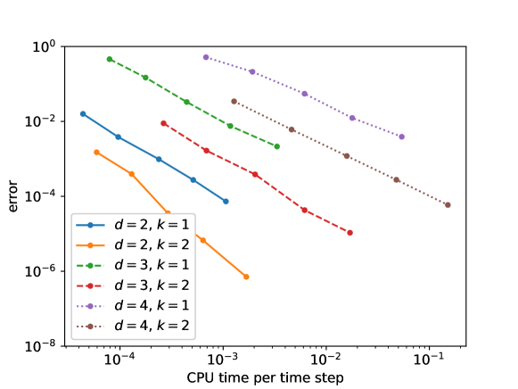
To further demonstrate the efficiency of the sparse grid algorithm, we report the errors versus the average CPU cost per time step for and in Fig. 4.1. It is observed that, to achieve a desired level of accuracy, the sparse grid DG method with a larger requires less CPU time as expected. Moreover, the CPU time is approximately proportional to the DOF. In addition, the slopes for all the lines in Fig. 4.1 are approximately the same with different dimensions. This indicates that our method has potential in the computations in high dimensions.
| DOF | -error | order | DOF | -error | order | |||
|---|---|---|---|---|---|---|---|---|
| 5 | 448 | 1.59e-2 | - | 4 | 432 | 1.50e-3 | - | |
| 6 | 1024 | 3.84e-3 | 2.05 | 5 | 1008 | 3.95e-4 | 1.93 | |
| 7 | 2304 | 9.80e-4 | 1.97 | 6 | 2304 | 3.54e-5 | 3.48 | |
| 8 | 5120 | 2.75e-4 | 1.84 | 7 | 5184 | 6.70e-6 | 2.40 | |
| 9 | 11264 | 7.33e-5 | 1.91 | 8 | 11520 | 7.10e-7 | 3.24 | |
| 4 | 832 | 4.60e-1 | - | 4 | 2808 | 8.92e-3 | - | |
| 5 | 2176 | 1.48e-1 | 1.63 | 5 | 7344 | 1.66e-3 | 2.42 | |
| 6 | 5504 | 3.30e-2 | 2.16 | 6 | 18576 | 3.85e-4 | 2.11 | |
| 7 | 13568 | 7.55e-3 | 2.13 | 7 | 45792 | 4.29e-5 | 3.17 | |
| 8 | 32768 | 2.15e-3 | 1.82 | 8 | 110592 | 1.07e-5 | 2.00 | |
| 5 | 8832 | 5.19e-1 | - | 4 | 15552 | 3.44e-2 | - | |
| 6 | 24320 | 2.12e-1 | 1.29 | 5 | 44712 | 6.08e-3 | 2.50 | |
| 7 | 64768 | 5.50e-2 | 1.94 | 6 | 123120 | 1.20e-3 | 2.35 | |
| 8 | 167936 | 1.24e-2 | 2.15 | 7 | 327888 | 2.77e-4 | 2.11 | |
| 9 | 425984 | 3.91e-3 | 1.66 | 8 | 850176 | 5.90e-5 | 2.23 | |
4.2 Hamilton-Jacobi equation
In this example, we consider the following Hamilton-Jacobi-Bellman (HJB) equation [7]
| (4.3) |
where and is a set of vectors corresponding to possible controls. The function is given by
| (4.4) |
with . Note that this HJB equation is equivalent to the following HJ equation
| (4.5) |
The exact solution can be hence derived from (4.5):
Here, for a vector , in the component-wise sense. We apply the adaptive algorithm to simulate (4.5). The outflow boundary conditions are imposed. Note that the Hamiltonian is nonsmooth and in [21] we regularize the absolute function to ensure stability:
| (4.6) |
It can be easily verified that is . In the simulation, we choose , where is the mesh size, and hence the regularization will not affect the accuracy of the original method.
This numerical test has been already examined in [21] by a local DG (LDG) method and here, we only present the sample code and focus on the CPU time study. The code is included in the GitHub repository ./example/04_hamilton_jacobi_adapt_hjb.cpp. Due to the page limit, we will only present the time evolution code.
The first part in the time evolution is to compute the time step size based on the finest mesh size in all the dimensions. Note that we use adaptive finite element space, so the finest mesh size is changing during the time evolution. The second part is to use the Euler forward time stepping to predict the numerical solution in the next time step. Here we use the LDG method in [35] to reconstruct the first-order derivatives of , i.e., , . In particular, the LDG method computes two auxiliary variables in each dimension, which approximate the first-order derivatives with opposite one-sided numerical fluxes. Therefore, there are totally unknown variables in the scheme including the unknown and the other auxiliary variables. For the auxiliary variables, the LDG bilinear forms are linear, and we evolve them by assembling the matrices stored in grad_linear in the code. For the evolution of , we first use Lagrangian interpolation basis to approximate the nonlinear Hamiltonian nonlinear_Lagr_fast and then apply fast matrix-vector multiplication. Since the assembling matrix is independent for each auxiliary variable, we use OpenMP here to improve the computational efficiency. After this, we call the function and then rhs_nonlinear to evaluate the residual (i.e. the right-hand-side of the weak formulation of and then call the time integrator to update the solution in the next time step.
The third part is to refine the numerical solution based on the prediction. After this refinement, the fourth part is to do the time evolution using the third-order SSP RK method [30]. Note that this part is similar to the prediction part by calling the same function. The only difference is to use RK3SSP instead of ForwardEuler. In the end of the time evolution, we do coarsening to remove the redundant elements.
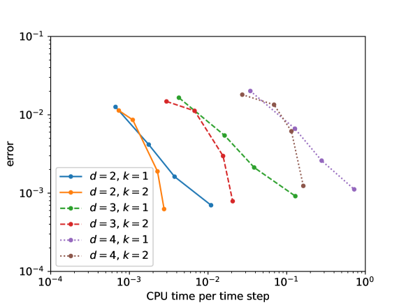
In this example, the viscosity solution is , a rarefaction wave opens up at the center of the domain, which is well captured by the adaptive sparse method, see the solution profile in [21]. In Table 4.3, we summarize the convergence study for and . Note that when , the error does not decay, and the reason is that the error has saturated already with the maximum level . In Figure 4.2, we plot the errors versus the average CPU cost per time step. It is again observed that, the errors with larger polynomial degree decays faster when reducing the refinement threshold and thus increasing DOF. The slopes with the same polynomial degrees in Figure 4.2 are almost the same with different dimensions. This again domenstrates the capability of our method in high dimensions.
| DOF | L2-error | DOF | L2-error | ||||||
|---|---|---|---|---|---|---|---|---|---|
| 1e-3 | 204 | 4.17e-3 | - | - | 63 | 8.62e-3 | - | - | |
| 1e-4 | 444 | 1.62e-3 | 0.41 | 1.21 | 135 | 1.89e-3 | 0.66 | 1.99 | |
| 1e-5 | 860 | 7.01e-4 | 0.36 | 1.27 | 207 | 6.26e-4 | 0.48 | 2.59 | |
| 1e-6 | 876 | 6.43e-4 | 0.04 | 4.69 | 459 | 4.24e-4 | 0.17 | 0.49 | |
| 1e-3 | 608 | 5.44e-3 | - | - | 270 | 1.12e-2 | - | - | |
| 1e-4 | 1328 | 2.12e-3 | 0.41 | 1.20 | 594 | 2.98e-3 | 0.58 | 1.68 | |
| 1e-5 | 2576 | 9.15e-4 | 0.37 | 1.27 | 918 | 7.89e-4 | 0.58 | 3.05 | |
| 1e-6 | 2624 | 8.39e-4 | 0.04 | 4.74 | 2052 | 4.36e-4 | 0.26 | 0.74 | |
| 1e-3 | 1616 | 6.65e-3 | - | - | 1053 | 1.35e-2 | - | - | |
| 1e-4 | 3536 | 2.60e-3 | 0.41 | 1.20 | 1701 | 6.17e-3 | 0.34 | 1.63 | |
| 1e-5 | 6864 | 1.12e-3 | 0.37 | 1.27 | 2997 | 1.24e-3 | 0.70 | 2.84 | |
| 1e-6 | 6992 | 1.02e-3 | 0.04 | 4.69 | 6237 | 4.90e-4 | 0.40 | 1.26 | |
4.3 Wave equation
In this example, we consider the isotropic wave propagation in heterogeneous media [11] in the domain with periodic boundary conditions:
| (4.7) |
For 2D case, the domain is composed of two subdomains and . The coefficient is a constant in each subdomain:
| (4.8) |
With this setup, the exact solution is a standing wave
| (4.9) |
For 3D case, and
| (4.10) |
In this case, the exact solution is a standing wave
| (4.11) |
This numerical example has been presented in [23]. Here, we show the sample code and focus more on the CPU cost study.
The main code is included in the GitHub repository ./example/03_wave_02_heter_media.cpp. Since the refinement and coarsening procedures are the same as the Hamilton-Jacobi equation, we only present the time evolution part. Here, we use the interior penalty DG [3] for the spatial discretization. In the weak formulation, we assemble the matrix for the linear part where is the penalty constant, is the mesh size, is the solution and is the test function. Then, we use Lagrangian interpolation to approximate , , and and apply fast matrix-vector multiplication to evaluate the residual terms.
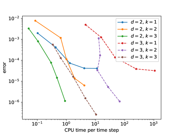
In Table 4.4, we show the convergence study for and . For with , the errors saturate because we use . Moreover, to reach the same magnitude of error, the DOF with higher polynomial degree will be much less that that with lower polynomial degree. In Figure 4.3, we plot the errors versus the average CPU cost per time step. It is again observed that, the errors with larger polynomial degree decays faster when reducing the refinement threshold and thus increasing DOF. The slopes with the same polynomial degrees in Figure 4.3 are almost the same with different dimensions. This indicates that the proposed method is resistant to the curse of dimensionality.
| DOF | -error | DOF | -error | ||||||
|---|---|---|---|---|---|---|---|---|---|
| 1e-1 | 784 | 1.97e-3 | - | - | 3840 | 4.96e-3 | - | - | |
| 1e-2 | 2816 | 4.17e-4 | 0.68 | 1.22 | 16832 | 1.24e-3 | 0.60 | 0.94 | |
| 1e-3 | 8496 | 7.31e-5 | 0.76 | 1.58 | 70656 | 1.37e-4 | 0.96 | 1.54 | |
| 1e-4 | 24384 | 4.18e-5 | 0.24 | 0.53 | 249664 | 3.86e-5 | 0.55 | 1.00 | |
| 1e-5 | 56960 | 4.10e-5 | 0.01 | 0.02 | 862528 | 3.19e-5 | 0.08 | 0.15 | |
| 1e-1 | 3204 | 7.72e-3 | - | - | 5238 | 1.12e-3 | - | - | |
| 1e-2 | 13842 | 1.17e-3 | 0.82 | 1.29 | 16794 | 1.71e-4 | 0.82 | 1.61 | |
| 1e-3 | 23544 | 1.12e-4 | 1.02 | 4.42 | 43416 | 3.33e-5 | 0.71 | 1.72 | |
| 1e-4 | 40320 | 1.39e-5 | 0.91 | 3.88 | 117558 | 5.32e-6 | 0.80 | 1.84 | |
| 1e-5 | 75042 | 6.32e-6 | 0.34 | 1.26 | 691632 | 1.10e-6 | 0.69 | 1.73 | |
| 1e-1 | 1472 | 3.29e-3 | - | - | 2304 | 5.59e-4 | - | - | |
| 1e-2 | 3904 | 8.00e-5 | 0.61 | 1.45 | 7040 | 1.28e-4 | 0.64 | 1.32 | |
| 1e-3 | 8256 | 7.71e-5 | 1.02 | 3.13 | 18176 | 1.65e-5 | 0.89 | 2.16 | |
| 1e-4 | 23488 | 1.47e-5 | 0.72 | 1.58 | 41472 | 1.55e-6 | 1.03 | 2.87 | |
| 1e-5 | 39360 | 1.15e-6 | 1.11 | 4.94 | 92928 | 2.58e-7 | 0.78 | 2.22 | |
5 Conclusions and future work
In this paper, we showcased the main components of our adaptive sparse grid DG C++ package AdaM-DG for solving PDEs. We focused on the details of the implementation, including the data structure, assembling of the operators, fast algorithms, and further demonstrated how to implement the package by three examples.
We would like to emphasize that this is still an on-going project, and many efforts are still needed to improve the software in various aspects. In particular, in the near term, we would like to improve some details of the code, including a more flexible definition of the computational domain, C++ implementation to further improve the memory and CPU time efficiency, a clear and comprehensive code documentation, a user-friendly Python interface, and a more efficient linear/nonlinear solver such as PETSc [5]. More importantly, we would like to generalize the code to an HPC platform with efficient parallel implementations on multicore CPU (using MPI) and GPU (using CUDA). Many aspects of the computational algorithms can also be further developed, including the hybridization with other numerical discretizations and a multi-domain approach which is more friendly to heterogeneous computing architecture.
Acknowledgements
We acknowledge the High Performance Computing Center (HPCC) at Michigan State University for providing computational resources that have contributed to the research results reported within this paper. We also would like to thank Kai Huang from Michigan State University, Yuan Liu from Wichita State University, Zhanjing Tao from Jilin University, and Qi Tang from Los Alamos National Laboratory for the assistance and discussion in the code implementation.
References
- [1] ASGarD - Adaptive Sparse Grid Discretization. https://github.com/project-asgard/asgard, 2022. Accessed on 10.18.2022.
- [2] B. K. Alpert. A class of bases in 2 for the sparse representation of integral operators. SIAM Journal on Mathematical Analysis, 24(1):246–262, 1993.
- [3] D. Arnold. An interior penalty finite element method with discontinuous elements. SIAM J. Numer. Anal., 19(4):742–760, 1982.
- [4] A. B. Atanasov and E. Schnetter. Sparse grid discretizations based on a discontinuous Galerkin method. arXiv preprint arXiv:1710.09356, 2017.
- [5] S. Balay, S. Abhyankar, M. Adams, J. Brown, P. Brune, K. Buschelman, L. Dalcin, A. Dener, V. Eijkhout, W. Gropp, et al. PETSc users manual. 2019.
- [6] R. Bellman. Adaptive control processes: a guided tour, volume 4. Princeton University Press Princeton, 1961.
- [7] O. Bokanowski, J. Garcke, M. Griebel, and I. Klompmaker. An adaptive sparse grid semi-Lagrangian scheme for first order Hamilton-Jacobi Bellman equations. Journal of Scientific Computing, 55(3):575–605, 2013.
- [8] H.-J. Bungartz and M. Griebel. Sparse Grids. Acta Numerica, 13:147–269, 2004.
- [9] A. Chen, F. Li, and Y. Cheng. An ultra-weak discontinuous Galerkin method for Schrödinger equation in one dimension. Journal of Scientific Computing, 78(2):772–815, 2019.
- [10] Y. Cheng and C.-W. Shu. A discontinuous Galerkin finite element method for time dependent partial differential equations with higher order derivatives. Mathematics of computation, 77(262):699–730, 2008.
- [11] C.-S. Chou, C.-W. Shu, and Y. Xing. Optimal energy conserving local discontinuous Galerkin methods for second-order wave equation in heterogeneous media. Journal of Computational Physics, 272:88–107, 2014.
- [12] B. Cockburn, S. Hou, and C.-W. Shu. The Runge-Kutta local projection discontinuous Galerkin finite element method for conservation laws. IV. The multidimensional case. Mathematics of Computation, 54(190):545–581, 1990.
- [13] E. D’Azevedo, D. L. Green, and L. Mu. Discontinuous galerkin sparse grids methods for time domain maxwell’s equations. Computer Physics Communications, 256:107412, 2020.
- [14] J. Garcke and M. Griebel. Sparse grids and applications. Springer, 2013.
- [15] V. Gradinaru. Fourier transform on sparse grids: code design and the time dependent Schrödinger equation. Computing, 80(1):1–22, 2007.
- [16] M. Griebel. Sparse grids and related approximation schemes for higher dimensional problems. In Proceedings of the conference on foundations of computational mathematics, Santander, Spain, 2005.
- [17] M. Griebel and J. Hamaekers. Sparse grids for the Schrödinger equation. ESAIM: Mathematical Modelling and Numerical Analysis, 41(02):215–247, 2007.
- [18] G. Guennebaud, B. Jacob, et al. Eigen v3. http://eigen.tuxfamily.org, 2010.
- [19] W. Guo and Y. Cheng. A sparse grid discontinuous Galerkin method for high-dimensional transport equations and its application to kinetic simulations. SIAM Journal on Scientific Computing, 38(6):A3381–A3409, 2016.
- [20] W. Guo and Y. Cheng. An adaptive multiresolution discontinuous Galerkin method for time-dependent transport equations in multidimensions. SIAM Journal on Scientific Computing, 39(6):A2962–A2992, 2017.
- [21] W. Guo, J. Huang, Z. Tao, and Y. Cheng. An adaptive sparse grid local discontinuous Galerkin method for hamilton-jacobi equations in high dimensions. Journal of Computational Physics, 436:110294, 2021.
- [22] J. Huang and Y. Cheng. An adaptive multiresolution discontinuous galerkin method with artificial viscosity for scalar hyperbolic conservation laws in multidimensions. SIAM Journal on Scientific Computing, 42(5):A2943–A2973, 2020.
- [23] J. Huang, Y. Liu, W. Guo, Z. Tao, and Y. Cheng. An adaptive multiresolution interior penalty discontinuous galerkin method for wave equations in second order form. Journal of Scientific Computing, 85(1):1–31, 2020.
- [24] J. Huang, Y. Liu, Y. Liu, Z. Tao, and Y. Cheng. A class of adaptive multiresolution ultra-weak discontinuous galerkin methods for some nonlinear dispersive wave equations. SIAM Journal on Scientific Computing, 44(2):A745–A769, 2022.
- [25] L. Pareschi and G. Russo. Implicit–explicit runge–kutta schemes and applications to hyperbolic systems with relaxation. Journal of Scientific computing, 25(1):129–155, 2005.
- [26] D. Pflüger. Spatially Adaptive Sparse Grids for High-Dimensional Problems. Verlag Dr. Hut, München, Aug. 2010.
- [27] C. Schwab, E. Süli, and R. Todor. Sparse finite element approximation of high-dimensional transport-dominated diffusion problems. ESAIM: Mathematical Modelling and Numerical Analysis, 42(05):777–819, 2008.
- [28] J. Shen and L.-L. Wang. Sparse spectral approximations of high-dimensional problems based on hyperbolic cross. SIAM J. Numer. Anal., 48(3):1087–1109, 2010.
- [29] J. Shen and H. Yu. Efficient spectral sparse grid methods and applications to high-dimensional elliptic problems. SIAM J. Sci. Comput., 32(6):3228–3250, 2010.
- [30] C.-W. Shu and S. Osher. Efficient implementation of essentially non-oscillatory shock-capturing schemes. Journal of Computational Physics, 77(2):439–471, 1988.
- [31] Z. Tao, J. Huang, Y. Liu, W. Guo, and Y. Cheng. An adaptive multiresolution ultra-weak discontinuous galerkin method for nonlinear schrödinger equations. Communications on Applied Mathematics and Computation, 4(1):60–83, 2022.
- [32] Z. Tao, Y. Jiang, and Y. Cheng. An adaptive high-order piecewise polynomial based sparse grid collocation method with applications. Journal of Computational Physics, 433:109770, 2021.
- [33] Z. Wang, Q. Tang, W. Guo, and Y. Cheng. Sparse grid discontinuous Galerkin methods for high-dimensional elliptic equations. Journal of Computational Physics, 314:244–263, 2016.
- [34] G. Wanner and E. Hairer. Solving ordinary differential equations I, volume 375. Springer Berlin Heidelberg New York, 1996.
- [35] J. Yan and S. Osher. A local discontinuous Galerkin method for directly solving Hamilton–Jacobi equations. Journal of Computational Physics, 230(1):232–244, 2011.
- [36] C. Zenger. Sparse grids. In Parallel Algorithms for Partial Differential Equations, Proceedings of the Sixth GAMM-Seminar, volume 31, 1990.