Inferring independent sets of Gaussian variables after thresholding correlations

Abstract

We consider testing whether a set of Gaussian variables, selected from the data, is independent of the remaining variables. We assume that this set is selected via a very simple approach that is commonly used across scientific disciplines: we select a set of variables for which the correlation with all variables outside the set falls below some threshold. Unlike other settings in selective inference, failure to account for the selection step leads, in this setting, to excessively conservative (as opposed to anti-conservative) results. Our proposed test properly accounts for the fact that the set of variables is selected from the data, and thus is not overly conservative. To develop our test, we condition on the event that the selection resulted in the set of variables in question. To achieve computational tractability, we develop a new characterization of the conditioning event in terms of the canonical correlation between the groups of random variables. In simulation studies and in the analysis of gene co-expression networks, we show that our approach has much higher power than a “naive” approach that ignores the effect of selection.

Keywords: Selective inference, gene co-expression network, canonical correlation analysis, correlation thresholding.

1 Introduction

A vast statistical literature focuses on estimation of, and inference on, the sparsity structure of a covariance or correlation matrix (see, e.g. Bickel and Levina, (2008); Drton and Perlman, (2008); Lam and Fan, (2009); Rothman et al., (2009); Bien and Tibshirani, (2011); Cai and Yuan, (2012); Liu et al., (2012); Rothman, (2012); Xue et al., (2012); Zhao et al., (2012); Liu et al., (2014); Serra et al., (2018) and references therein). In this article, we focus on a particular type of sparsity in which the matrix has a block diagonal structure (up to a permutation of the rows and columns). This type of sparsity arises in a number of scientific fields. For example, in the study of gene co-expression networks, discovery of independent “gene sets” plays a pivotal role (e.g. Freeman et al., 2007). In genetics, discovery of haplotype blocks often reduces to partitioning the linkage disequilibrium matrix into approximately independent blocks (Patil et al.,, 2001). In neuroscience, it is of interest to discover correlated brain regions in brain functional connectivity networks (Bordier et al.,, 2017).

We consider a simple approach to estimating block diagonal structure in a correlation matrix. Our paper’s primary contribution is a novel approach to testing whether two sets of variables that appear in different estimated blocks are, in fact, uncorrelated. For example, is an estimated gene set in a gene co-expression network really uncorrelated with the remaining genes? This is a challenging question because the same data is used both to estimate the gene set and to test a hypothesis based on this estimated gene set. The problem falls into the selective inference framework, which has been studied in various other contexts by Fithian et al., (2014); Lee and Taylor, (2014); Loftus and Taylor, (2015); Lee et al., (2016); Yang et al., (2016); Tibshirani et al., (2016); Suzumura et al., (2017); Hyun et al., (2018); Tian et al., (2018); Hyun et al., (2018); Jewell et al., (2022); Chen and Bien, (2020); Gao et al., (2022); Neufeld et al., (2021); Chen and Witten, (2022), among others. However, unlike those other papers, in our setting, failure to account for double-use of data leads to a loss of power rather than loss of type I error control.

The rest of this paper is organized as follows. In Section 2, we briefly review some results related to testing hypotheses associated with submatrices of a covariance matrix, define the notion of selective type I error in this context, and then provide a general expression for constructing p-values that are valid in this selective sense. In Section 3, we present a data-adaptive procedure for estimating diagonal blocks in a correlation matrix, and consider testing the null hypothesis of no correlation between an estimated block and the remaining variables. Furthermore, we show that the event corresponding to the selection of a particular hypothesis can be characterized analytically. In Section 4, we apply this characterization to develop a selective inference approach to test the null hypothesis of interest. Simulation results in Section 5 and an analysis of gene co-expression networks in Section 6 demonstrate the value of the proposed approach. We close with a discussion in Section 7.

2 Problem definition

2.1 Hypothesis testing for pre-specified groups of variables

For a positive definite $p\times p$ matrix $\Sigma$, consider a data matrix consisting of $n>p$ independent observations of a $p$-dimensional multivariate Gaussian,

$$\textbf{X}\sim\mathcal{MN}_{n\times p}\left(\mathbf{0},\mathbf{I}_{n},\mathbf{\mbox{\boldmath$\Sigma$}}_{p\times p}\right).$$ (1)

For a predetermined subset $\mathcal{P}\subset\left\{1,2,\ldots,p\right\}$ of variables, consider testing for dependence between the variables in $\mathcal{P}$ and the variables in its complement ${\mathcal{P}}^{c}:=\left\{1,2,\ldots,p\right\}\setminus\mathcal{P}$, i.e.

$$H_{0}^{\mathcal{P}}:\mbox{\boldmath$\Sigma$}_{{\mathcal{P}},{\mathcal{P}}^{c}}=\mathbf{0}\>\text{ versus }\>H_{1}^{\mathcal{P}}:\mbox{\boldmath$\Sigma$}_{{\mathcal{P}},{\mathcal{P}}^{c}}\neq\mathbf{0},$$ (2)

where $\mbox{\boldmath$\Sigma$}_{\mathcal{P}_{1},\mathcal{P}_{2}}$ denotes the submatrix of $\Sigma$ with rows in $\mathcal{P}_{1}$ and columns in $\mathcal{P}_{2}$. Given a realization $\textbf{x}\in\mathbb{R}^{n\times p}$ of X, the classical likelihood ratio test (LRT) of (2) yields the p-value

$$p_{\mathrm{LRT}}\left(\textbf{x};\mathcal{P}\right):=\mathbb{P}_{H_{0}^{\mathcal{P}}}\left(\frac{\left|\textbf{S}\left(\textbf{X}\right)\right|}{\left|\textbf{S}_{{\mathcal{P}},{\mathcal{P}}}\left(\textbf{X}\right)\right|\left|\textbf{S}_{{\mathcal{P}}^{c},{\mathcal{P}}^{c}}\left(\textbf{X}\right)\right|}\leqslant\frac{\left|\textbf{S}\left(\textbf{x}\right)\right|}{\left|\textbf{S}_{{\mathcal{P}},{\mathcal{P}}}\left(\textbf{x}\right)\right|\left|\textbf{S}_{{\mathcal{P}}^{c},{\mathcal{P}}^{c}}\left(\textbf{x}\right)\right|}\right),$$ (3)

where $\textbf{S}\left(\textbf{x}\right)=\frac{1}{n}\left(\textbf{x}-\mathbf{1}_{n}\bar{x}^{\top}\right)^{\top}\left(\textbf{x}-\mathbf{1}_{n}\bar{x}^{\top}\right)$ is the sample covariance matrix of x, $\bar{x}\in\mathbb{R}^{p}$ denotes the sample mean of x, and $\left|\textbf{M}\right|$ denotes the determinant of the matrix M (see (3) of Section 9.8 in Anderson, 2003). Here, $\textbf{S}_{\mathcal{P}_{1},\mathcal{P}_{2}}$ represents the submatrix of S with rows in $\mathcal{P}_{1}$ and columns in $\mathcal{P}_{2}$. The compact singular value decomposition (SVD) of the cross-covariance of decorrelated (“whitened”) versions of $\textbf{x}_{\mathcal{P}}$ and $\textbf{x}_{{\mathcal{P}}^{c}}$ (defined as the submatrices of x with columns in $\mathcal{P}$ and ${\mathcal{P}}^{c}$, respectively) can be written as

$$\mathbf{S}^{W}_{{\mathcal{P}},{\mathcal{P}}^{c}}\left(\textbf{x}\right):=\left(\textbf{S}_{{\mathcal{P}},{\mathcal{P}}}\left(\textbf{x}\right)\right)^{-\frac{1}{2}}\textbf{S}_{{\mathcal{P}},{\mathcal{P}}^{c}}\left(\textbf{x}\right)\left(\textbf{S}_{{\mathcal{P}}^{c},{\mathcal{P}}^{c}}\left(\textbf{x}\right)\right)^{-\frac{1}{2}}\overset{SVD}{=}\hat{\mathbf{A}}^{{\mathcal{P}}}\left(\textbf{x}\right)\>\hat{\bm{\Lambda}}^{{\mathcal{P}}}\left(\textbf{x}\right)\>\left({\hat{\mathbf{\Gamma}}^{{{\mathcal{P}}}}}\left(\textbf{x}\right)\right)^{\top},$$ (4)

where $\hat{\bm{\Lambda}}^{{\mathcal{P}}}\left(\textbf{x}\right):=\mathrm{diag}\left(\hat{\lambda}_{1}\left(\textbf{x}\right),\hat{\lambda}_{2}\left(\textbf{x}\right),\ldots,\hat{\lambda}_{r\left(\mathcal{P}\right)}\left(\textbf{x}\right)\right)$ is a square diagonal matrix of
$r\left(\mathcal{P}\right):=\min\left\{\mathrm{card}\left({\mathcal{P}}\right),\mathrm{card}\left({\mathcal{P}}^{c}\right)\right\}$ non-negative singular values in non-increasing order ($\hat{\lambda}_{1}\left(\textbf{x}\right)\geqslant\hat{\lambda}_{2}\left(\textbf{x}\right)\geqslant\ldots\geqslant\hat{\lambda}_{r\left(\mathcal{P}\right)}\left(\textbf{x}\right)\geqslant 0$) and $\hat{\mathbf{A}}^{{\mathcal{P}}}\left(\textbf{x}\right)$ and $\hat{\bm{\Gamma}}^{{\mathcal{P}}}\left(\textbf{x}\right)$ are the $\mathrm{card}\left({\mathcal{P}}\right)\times r\left(\mathcal{P}\right)$ and $\mathrm{card}\left({\mathcal{P}}^{c}\right)\times r\left(\mathcal{P}\right)$ matrices of left and right singular vectors, respectively. The diagonal elements of $\hat{\bm{\Lambda}}^{{\mathcal{P}}}\left(\textbf{x}\right)$ can be interpreted as the canonical correlations between $\textbf{x}_{{\mathcal{P}}}$ and $\textbf{x}_{{\mathcal{P}}^{c}}$, and the columns of $\left(\textbf{S}_{{\mathcal{P}},{\mathcal{P}}}\left(\textbf{x}\right)\right)^{-\frac{1}{2}}\hat{\mathbf{A}}^{{\mathcal{P}}}\left(\textbf{x}\right)$ and $\left(\textbf{S}_{{\mathcal{P}^{c}},{\mathcal{P}^{c}}}\left(\textbf{x}\right)\right)^{-\frac{1}{2}}\hat{\mathbf{\Gamma}}^{{{\mathcal{P}}}}\left(\textbf{x}\right)$ are the left and right canonical vectors.

Using the notation in (4), the LRT statistic in (3) can be rewritten as

$$\frac{\left|\textbf{S}\left(\textbf{x}\right)\right|}{\left|\textbf{S}_{{\mathcal{P}},{\mathcal{P}}}\left(\textbf{x}\right)\right|\left|\textbf{S}_{{\mathcal{P}}^{c},{\mathcal{P}}^{c}}\left(\textbf{x}\right)\right|}=\left|\textbf{I}_{r\left(\mathcal{P}\right)}-\left(\hat{\bm{\Lambda}}^{{\mathcal{P}}}\left(\textbf{x}\right)\right)^{2}\right|,$$ (5)

and the associated p-value can be rewritten as

$$p_{\mathrm{LRT}}\left(\textbf{x};\mathcal{P}\right)=\mathbb{P}_{H_{0}^{\mathcal{P}}}\left(\left|\textbf{I}_{r\left(\mathcal{P}\right)}-\left(\hat{\bm{\Lambda}}^{{\mathcal{P}}}\left(\textbf{X}\right)\right)^{2}\right|\leqslant\left|\textbf{I}_{r\left(\mathcal{P}\right)}-\left(\hat{\bm{\Lambda}}^{{\mathcal{P}}}\left(\textbf{x}\right)\right)^{2}\right|\right).$$ (6)

Details are in Supplementary Material Section S1. Under $H_{0}^{\mathcal{P}}$ and the assumption that $n>p$, the test statistic follows a Wilks’ lambda distribution (see page 288 of Mardia et al., 1979). We will later use Proposition 1 to sample from the Wilks’ lambda distribution to evaluate $p_{\mathrm{LRT}}\left(\textbf{x};\mathcal{P}\right)$ in (6).

Proposition 1.

Under $H_{0}^{\mathcal{P}}$ and the assumption that $n>p$, the following statements hold regarding the sample canonical correlations $\left(\hat{\lambda}_{1},\hat{\lambda}_{2},\ldots,\hat{\lambda}_{r\left(\mathcal{P}\right)}\right)$ defined in (4):

1. The sample canonical correlations have joint density,

   $$f\left(\hat{\lambda}_{1},\hat{\lambda}_{2},\ldots,\hat{\lambda}_{r\left(\mathcal{P}\right)}\right)= \pi^{\frac{1}{2}\left(r\left(\mathcal{P}\right)\right)^{2}}\frac{2^{r\left(\mathcal{P}\right)}\Gamma_{r\left(\mathcal{P}\right)}\left(\frac{n}{2}\right)}{\Gamma_{r\left(\mathcal{P}\right)}\left(\frac{n-p+r\left(\mathcal{P}\right)}{2}\right)\Gamma_{p}\left(\frac{1}{2}r\left(\mathcal{P}\right)\right)\Gamma_{p}\left(\frac{1}{2}\left(p-r\left(\mathcal{P}\right)\right)\right)}\times$$ (7)

   $$\prod_{i=1}^{r\left(\mathcal{P}\right)}\left\{\hat{\lambda}_{i}^{\left(p-2r\left(\mathcal{P}\right)\right)}\left(1-\hat{\lambda}_{i}^{2}\right)^{\frac{1}{2}\left(n-p-2\right)}\right\}\prod_{i<j}\left(\hat{\lambda}_{i}^{2}-\hat{\lambda}_{j}^{2}\right),$$

   supported on $\left\{1\geqslant\hat{\lambda}_{1}\geqslant\hat{\lambda}_{2}\geqslant\ldots\geqslant\hat{\lambda}_{r\left(\mathcal{P}\right)}\geqslant 0\right\}$.

2. The sample canonical correlations have the same distribution as
   $\left(\sqrt{\frac{\Psi_{1}}{1+\Psi_{1}}},\sqrt{\frac{\Psi_{2}}{1+\Psi_{2}}},\ldots,\sqrt{\frac{\Psi_{r\left(\mathcal{P}\right)}}{1+\Psi_{r\left(\mathcal{P}\right)}}}\right)$, where $\left(\Psi_{1},\Psi_{2},\ldots,\Psi_{r\left(\mathcal{P}\right)}\right)$ are the eigenvalues of $\mathbf{W}\mathbf{T}^{-1}$, for $\mathbf{W}\sim\mathrm{Wishart}_{r\left(\mathcal{{P}}\right)}\left(\mathbf{I}_{r\left(\mathcal{{P}}\right)},p-r\left(\mathcal{{P}}\right)\right)$, $\mathbf{T}\sim\mathrm{Wishart}_{r\left(\mathcal{{P}}\right)}\left(\mathbf{I}_{r\left(\mathcal{{P}}\right)},n-1-p+r\left(\mathcal{{P}}\right)\right)$, and $\mathbf{W}\mathchoice{\mathrel{\hbox to0.0pt{$\displaystyle\perp$\hss}\mkern 2.0mu{\displaystyle\perp}}}{\mathrel{\hbox to0.0pt{$\textstyle\perp$\hss}\mkern 2.0mu{\textstyle\perp}}}{\mathrel{\hbox to0.0pt{$\scriptstyle\perp$\hss}\mkern 2.0mu{\scriptstyle\perp}}}{\mathrel{\hbox to0.0pt{$\scriptscriptstyle\perp$\hss}\mkern 2.0mu{\scriptscriptstyle\perp}}}\mathbf{T}$.

3. If $r\left({\mathcal{P}}\right)=1$, then the sample canonical correlation $\hat{\lambda}_{1}$ is the sample multiple correlation coefficient for the regression of the single variable onto the remaining $p-1$ variables, and

   $$\hat{\lambda}_{1}^{2}\sim\mathrm{Beta}\left(\frac{p-1}{2},\frac{n-p}{2}\right).$$ (8)

Here, (i) gives us the joint density of $\left(\hat{\lambda}_{1},\hat{\lambda}_{2},\ldots,\hat{\lambda}_{r\left(\mathcal{P}\right)}\right)$. In Section 4, we will use (ii) to sample from the joint distribution of $\left(\hat{\lambda}_{1},\hat{\lambda}_{2},\ldots,\hat{\lambda}_{r\left(\mathcal{P}\right)}\right)$, as the joint density in (i) is not amenable to sampling. We will make use of (iii) to bypass sampling in the special case of $r\left({\mathcal{P}}\right)=1$. We defer the proof of Proposition 1 to Supplementary Material Section S2. Crucially, under $H_{0}^{\mathcal{P}}$, the distribution of the sample canonical correlations depends only on $n$, $p$, and $r\left({\mathcal{P}}\right)$.

Next, we explore how the situation changes if we consider a data-dependent subset of variables, instead of a predetermined one as in the case of (2).

2.2 What changes when the groups of variables are chosen from the data?

We now suppose that $\mathcal{P}$ is a function of the data, and specifically of $\textbf{S}\left(\textbf{x}\right)$. That is, we define $\mathcal{P}:\mathcal{S}_{++}^{p}\mapsto\mathcal{B}_{p}$, where $\mathcal{S}_{++}^{p}$ denotes the set of all symmetric positive definite matrices, and $\mathcal{B}_{p}$ denotes the set of all possible partitions of $\left\{1,2,\ldots,p\right\}$. For $\hat{\mathcal{P}}\in\mathcal{P}\left(\textbf{S}\left(\textbf{x}\right)\right)$, we wish to test

$$H_{0}^{\hat{\mathcal{P}}}:\mbox{\boldmath$\Sigma$}_{\hat{\mathcal{P}},\hat{\mathcal{P}}^{c}}=\mathbf{0}\>\>\>\>\text{versus}\>\>\>H_{1}^{\hat{\mathcal{P}}}:\mbox{\boldmath$\Sigma$}_{\hat{\mathcal{P}},\hat{\mathcal{P}}^{c}}\neq\mathbf{0}.$$ (9)

We assume without loss of generality that $\hat{\mathcal{P}}=\left\{1,2,\ldots,\mathrm{card}\left({\hat{\mathcal{P}}}\right)\right\}$ and
$\hat{\mathcal{P}}^{c}=\left\{\mathrm{card}\left({\hat{\mathcal{P}}}\right)+1,\ldots,p\right\}$. Since $\hat{\mathcal{P}}\in\mathcal{P}\left(\textbf{S}\left(\textbf{x}\right)\right)$, the null hypothesis in (9) is a function of the data. The classical test statistic in (3) does not follow a Wilks’ lambda distribution under the null hypothesis (9). Ignoring this fact can lead to a tremendous loss of power. To demonstrate this in an example, we simulate data with $p=6$ and $n=9$ for a completely dense $\Sigma$, so that $H_{1}^{\hat{\mathcal{P}}}:\mbox{\boldmath$\Sigma$}_{\hat{\mathcal{P}},\hat{\mathcal{P}}^{c}}\neq\mathbf{0}$ holds for all $\hat{\mathcal{P}}$. Figures 1(a)-(b) display the heatmaps of the absolute values of the entries of the population correlation matrix and the sample correlation matrix. We tested (9) for $\hat{\mathcal{P}}$ obtained via the thresholding procedure described in Algorithm 1; this yielded $\hat{\mathcal{P}}=\left\{1,2,3\right\}$. Ignoring that $\hat{\mathcal{P}}$ was selected based on the data and using Wilks’ lambda as the reference distribution for the likelihood ratio test statistic yielded a p-value $\left(p_{\mathrm{LRT}}\right)$ of $0.773$, whereas our proposed selective inference approach produced a p-value of $0.015$. Figure 1(c) shows the distribution of p-values over $10,000$ data realizations using the two approaches. We see that our selective p-values tend to be small — as expected, since the null hypothesis does not hold — whereas the classical p-values are stochastically greater than a uniform.

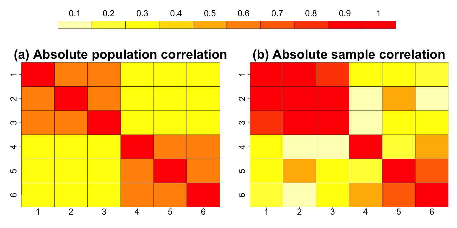
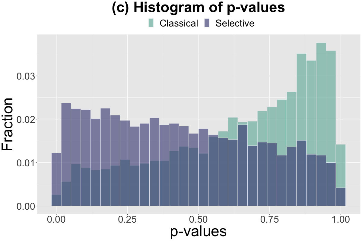
Figure 1: Heatmap of the absolute values of the entries of the (a) population correlation matrix and (b) sample correlation matrix, for $p=6$ and $n=9$. Histograms of the classical LRT p-values and the selective LRT p-values are in (c).

At first glance, the fact that the classical test has low power in this scenario may seem counter-intuitive, since failure to account for selection typically leads to an inflated type I error rate, as opposed to low power, in related settings (Fithian et al.,, 2014). However, in this setting, the procedure $\mathcal{P}\left(\cdot\right)$ that selects $\hat{\mathcal{P}}$ (as described in Algorithm 1) does so because of its low correlation with $\hat{\mathcal{P}}^{c}$. Thus, the likelihood ratio test statistic will be stochastically greater than the Wilks’ lambda distribution under $H_{0}^{\hat{\mathcal{P}}}:\mbox{\boldmath$\Sigma$}_{\hat{\mathcal{P}},\hat{\mathcal{P}}^{c}}=\mathbf{0}$, yielding an overly conservative p-value.

2.3 Selective inference for the covariance matrix

Fithian et al., (2014) argues that when a null hypothesis is selected from the data, we should control the probability of a false rejection conditional on having selected this null hypothesis, i.e. the selective type I error rate. In the context of (9), the selective type I error rate is defined as follows:

Definition 1.

(Selective type I error) A test of $H_{0}^{\mathcal{R}}:\mbox{\boldmath$\Sigma$}_{\mathcal{R},\mathcal{R}^{c}}=\mathbf{0}$ controls the selective type I error if, for every subset ${\mathcal{R}}$ of $\left\{1,2,\ldots,p\right\}$,

$$\mathbb{P}_{H_{0}^{{\mathcal{R}}}}\left(\text{reject }H_{0}^{{\mathcal{R}}}\text{ at level }\alpha\bigg{|}{\mathcal{R}}\in\mathcal{P}\left(\mathbf{S}\left(\mathbf{X}\right)\right)\right)\leqslant\alpha;\>\forall\>0\leqslant\alpha\leqslant 1.$$ (10)

By the probability integral transform, it can be shown that a conditional version of (6),

$$p_{0}\left(\textbf{x};\hat{\mathcal{P}}\right):=\mathbb{P}_{H_{0}^{\hat{\mathcal{P}}}}\left(\left|\textbf{I}-\left(\hat{\bm{\Lambda}}^{\hat{\mathcal{P}}}\left(\textbf{X}\right)\right)^{2}\right|\leqslant\left|\textbf{I}-\left(\hat{\bm{\Lambda}}^{\hat{\mathcal{P}}}\left(\textbf{x}\right)\right)^{2}\right|\bigg{|}\hat{\mathcal{P}}\in\mathcal{P}\left(\textbf{S}\left(\textbf{X}\right)\right)\right),$$ (11)

controls the selective type I error in (10). However, (11) is not computationally tractable, because the distribution of $\left|\textbf{I}-\left(\hat{\bm{\Lambda}}^{\hat{\mathcal{P}}}\left(\textbf{X}\right)\right)^{2}\right|$, conditional on $\hat{\mathcal{P}}\in\mathcal{P}\left(\textbf{S}\left(\textbf{X}\right)\right)$, depends on parameters that are unknown even under the null hypothesis. To bypass this problem, we employ a common approach in the selective inference literature (see e.g. Lee et al., 2016), in which we condition on some additional information. In particular, we propose a p-value for $H_{0}^{\hat{\mathcal{P}}}$ as

$$p\left(\textbf{x};\hat{\mathcal{P}}\right):=\mathbb{P}_{H_{0}^{\hat{\mathcal{P}}}}\bigg{(}\left|\textbf{I}-\left(\hat{\bm{\Lambda}}^{\hat{\mathcal{P}}}\left(\textbf{X}\right)\right)^{2}\right|\leqslant\left|\textbf{I}-\left(\hat{\bm{\Lambda}}^{\hat{\mathcal{P}}}\left(\textbf{x}\right)\right)^{2}\right|\bigg{|} \hat{\mathcal{P}}\in\mathcal{P}\left(\textbf{S}\left(\textbf{X}\right)\right),$$ (12)

$$\textbf{S}_{\hat{\mathcal{P}},\hat{\mathcal{P}}}\left(\textbf{X}\right)=\textbf{S}_{\hat{\mathcal{P}},\hat{\mathcal{P}}}\left(\textbf{x}\right),\textbf{S}_{\hat{\mathcal{P}}^{c},\hat{\mathcal{P}}^{c}}\left(\textbf{X}\right)=\textbf{S}_{\hat{\mathcal{P}}^{c},\hat{\mathcal{P}}^{c}}\left(\textbf{x}\right), \>\hat{\mathbf{A}}^{\hat{\mathcal{P}}}\left(\textbf{X}\right)=\hat{\mathbf{A}}^{\hat{\mathcal{P}}}\left(\textbf{x}\right),\hat{\bm{\Gamma}}^{\hat{\mathcal{P}}}\left(\textbf{X}\right)=\hat{\bm{\Gamma}}^{\hat{\mathcal{P}}}\left(\textbf{x}\right)\bigg{)},$$

where we recall the SVD in (4). The intuition behind this conditioning set is as follows:

1. Fixed within-group covariance: Due to the nature of the null hypothesis in (9), we are primarily interested in inter-group correlation. Hence we keep the intra-group covariance fixed, i.e., we only consider X for which $\textbf{S}_{\hat{\mathcal{P}},\hat{\mathcal{P}}}\left(\textbf{X}\right)=\textbf{S}_{\hat{\mathcal{P}},\hat{\mathcal{P}}}\left(\textbf{x}\right)$ and $\textbf{S}_{\hat{\mathcal{P}}^{c},\hat{\mathcal{P}}^{c}}\left(\textbf{X}\right)=\textbf{S}_{\hat{\mathcal{P}}^{c},\hat{\mathcal{P}}^{c}}\left(\textbf{x}\right)$.

2. Fixed between-group distance direction: Inspecting (4) and (5), we see that the only part of $\mathbf{S}^{W}_{\hat{\mathcal{P}},\hat{\mathcal{P}}^{c}}$ that is involved in the test statistic is $\hat{\bm{\Lambda}}^{\hat{\mathcal{P}}}$. The left and right singular vectors of $\mathbf{S}^{W}_{\hat{\mathcal{P}},\hat{\mathcal{P}}^{c}}$ in (4), i.e. $\hat{\mathbf{A}}^{\hat{\mathcal{P}}}$ and $\hat{\bm{\Gamma}}^{\hat{\mathcal{P}}}$, are not involved in the test statistic. Hence, in (12), we only consider X for which $\hat{\mathbf{A}}^{\hat{\mathcal{P}}}\left(\textbf{X}\right)=\hat{\mathbf{A}}^{\hat{\mathcal{P}}}\left(\textbf{x}\right)$ and $\hat{\bm{\Gamma}}^{\hat{\mathcal{P}}}\left(\textbf{X}\right)=\hat{\bm{\Gamma}}^{\hat{\mathcal{P}}}\left(\textbf{x}\right)$.

The next theorem establishes that the conditioning set in (12) can be written in terms of constraints on the sample canonical correlations, and that $p\left(\mathbf{x};\hat{\mathcal{P}}\right)$ controls the selective type I error rate.

Theorem 1.

For any realization $\mathbf{x}$ of $\mathbf{X}$ in (1) and for an arbitrary subset $\mathcal{R}$ of $\left\{1,2,\ldots,p\right\}$, we can express $p\left(\mathbf{x};{\mathcal{R}}\right)$ defined in (12) as

$$p\left(\mathbf{x};{\mathcal{R}}\right)=\mathbb{P}_{H_{0}^{\mathcal{R}}}\left(\prod_{i=1}^{r\left({\mathcal{R}}\right)}\left(1-\lambda_{i}^{2}\right)\leqslant\prod_{i=1}^{r\left({\mathcal{R}}\right)}\left(1-\left(\hat{\lambda}_{i}^{\mathcal{R}}\left(\mathbf{x}\right)\right)^{2}\right)\bigg{|}\left(\lambda_{1},\lambda_{2},\ldots,\lambda_{r\left({\mathcal{R}}\right)}\right)\in{\mathcal{G}}\left(\mathbf{x};{\mathcal{R}}\right)\right),$$ (13)

where $\left\{\lambda_{i}\right\}_{i=1}^{r\left({\mathcal{R}}\right)}$ has joint density $f\left(\lambda_{1},\lambda_{2},\ldots,\lambda_{r\left({\mathcal{R}}\right)}\right)$ defined in (7), $\left\{\hat{\lambda}_{i}^{\mathcal{R}}\left(\mathbf{x}\right)\right\}_{i=1}^{r\left({\mathcal{R}}\right)}$ are the diagonal entries of $\hat{\bm{\Lambda}}^{\mathcal{R}}\left(\mathbf{x}\right)$, and

$${\mathcal{G}}\left(\mathbf{x};{\mathcal{R}}\right):=\left\{\left(\lambda_{1},\lambda_{2},\ldots,\lambda_{r\left({\mathcal{R}}\right)}\right)\in[0,1]^{r\left({\mathcal{R}}\right)}:\lambda_{1}\geqslant\lambda_{2}\geqslant\ldots\geqslant\lambda_{r\left({\mathcal{R}}\right)};{\mathcal{R}}\in\mathcal{P}\left(\mathbf{S}^{\prime}\left(\mathbf{x},{{\mathcal{R}}},\left\{\lambda_{i}\right\}_{i=1}^{r\left({\mathcal{R}}\right)}\right)\right)\right\},$$ (14)

where $\mathbf{S}^{\prime}\left(\mathbf{x},{\mathcal{R}},\left\{\lambda_{i}\right\}_{i=1}^{r\left({\mathcal{R}}\right)}\right)$ is a modified version of the sample covariance matrix with a perturbed off-diagonal block,

$$\mathbf{S}_{{\mathcal{R}},{\mathcal{R}}^{c}}^{\prime}\left(\mathbf{x},{\mathcal{R}},\left\{\lambda_{i}\right\}_{i=1}^{r\left({\mathcal{R}}\right)}\right):=\left(\mathbf{S}_{{\mathcal{R}},{\mathcal{R}}}\left(\mathbf{x}\right)\right)^{\frac{1}{2}}\hat{\mathbf{A}}^{{\mathcal{R}}}\left(\mathbf{x}\right)\mathrm{diag}\left(\lambda_{1},\lambda_{2},\ldots,\lambda_{r\left({\mathcal{R}}\right)}\right)\left(\hat{\mathbf{\Gamma}}^{{\mathcal{R}}}\left(\mathbf{x}\right)\right)^{\top}\left(\mathbf{S}_{{\mathcal{R}}^{c},{\mathcal{R}}^{c}}\left(\mathbf{x}\right)\right)^{\frac{1}{2}}.$$ (15)

Furthermore, rejecting $H_{0}^{{\mathcal{R}}}$ if $p\left(\mathbf{x};{\mathcal{R}}\right)\leqslant\alpha$ controls the selective type I error rate at level $\alpha$, i.e.

$$\mathbb{P}_{H_{0}^{{\mathcal{R}}}}\left(p\left(\mathbf{X};{\mathcal{R}}\right)\leqslant\alpha\bigg{|}{\mathcal{R}}\in\mathcal{P}\left(\mathbf{S}\left(\mathbf{X}\right)\right)\right)\leqslant\alpha;\>\forall\>0\leqslant\alpha\leqslant 1.$$ (16)

Recall that $\hat{\mathbf{A}}^{{\mathcal{R}}}\left(\mathbf{x}\right),\hat{\bm{\Lambda}}^{{\mathcal{R}}}\left(\mathbf{x}\right)$ and $\hat{\bm{\Gamma}}^{{\mathcal{R}}}\left(\mathbf{x}\right)$ were defined in (4). We defer the proof of Theorem 1 to Supplementary Material Section S3. Theorem 1 demonstrates that computation of the p-value in (12) boils down to characterizing ${\mathcal{G}}\left(\mathbf{x};\hat{\mathcal{P}}\right)$ in (14).

Furthermore, ${\mathcal{G}}\left(\mathbf{x};\hat{\mathcal{P}}\right)$ in (14) describes the points $\left\{\lambda_{i}\right\}_{i=1}^{r\left(\hat{\mathcal{P}}\right)}$ in the $r\left(\hat{\mathcal{P}}\right)$-dimensional unit hyper-cube for which the coordinates are in non-increasing order, and for which applying a variable grouping method $\mathcal{P}\left(\cdot\right)$ to the perturbed covariance matrix $\mathbf{S}^{\prime}\left(\mathbf{x},\hat{\mathcal{P}},\left\{\lambda_{i}\right\}_{i=1}^{r\left(\hat{\mathcal{P}}\right)}\right)$ yields $\hat{\mathcal{P}}$. Characterization of this set depends on the procedure used for obtaining the block diagonal structure of the correlation matrix, i.e. on $\mathcal{P}\left(\cdot\right)$. In the next section, we focus on a specific data-adaptive procedure for $\mathcal{P}\left(\cdot\right)$, and on the corresponding characterization of ${\mathcal{G}}\left(\mathbf{x};\hat{\mathcal{P}}\right)$ in (14).

3 Characterization of the conditioning set

3.1 Procedure for obtaining groups of uncorrelated variables

We present a simple procedure for identifying groups of uncorrelated variables, i.e., for discovering block diagonal structure of the covariance matrix. We assume that there are no ties between the off-diagonal entries of the sample correlation matrix, which holds with probability $1$. We denote the correlation matrix corresponding to the sample covariance matrix $\textbf{S}=\textbf{S}\left(\textbf{x}\right)$ as $\mathbf{R}\left(\mathbf{S}\right)$, with $\left(i,j\right)^{th}$ element $\textbf{R}_{i,j}\left(\textbf{S}\right)=\frac{\textbf{S}_{i,j}}{\sqrt{\textbf{S}_{i,i}\textbf{S}_{j,j}}}$, for $i,j\in\left\{1,2,\ldots,p\right\}$. Let $\mathds{1}\left\{\mathcal{A}\right\}$ denote the indicator function of the event $\mathcal{A}$. Algorithm 1 summarizes the procedure for obtaining groups of uncorrelated variables. Note that if the variables have an intrinsic ordering, then in line 5 of Algorithm 1 we discard groups of variables that violate that ordering.

Algorithm 1 Procedure for obtaining groups of uncorrelated variables

Input: Sample covariance matrix $\textbf{S}\left(\textbf{x}\right)$; threshold $c$.

1:procedure 

2:     Create the adjacency matrix $\mathbf{D}_{i,j}=\mathds{1}\left\{\left|\textbf{R}_{i,j}\left(\textbf{S}\left(\textbf{x}\right)\right)\right|>c\right\}$;

3:     Identify the connected components $\mathcal{C}_{1},\mathcal{C}_{2},\ldots,\mathcal{C}_{K}$ of the graph corresponding to the
      adjacency matrix;

4:     if variables are ordered then

5:         $\mathcal{P}\left(\textbf{S}\left(\textbf{x}\right)\right)=\left\{\mathcal{C}_{k}:\mathcal{C}_{k}\text{ consists exclusively of consecutive variables}\right\}$;

6:     else

7:         $\mathcal{P}\left(\textbf{S}\left(\textbf{x}\right)\right)=\left\{\mathcal{C}_{1},\mathcal{C}_{2},\ldots,\mathcal{C}_{K}\right\}$.      

3.2 Calculation of the conditioning set

In this subsection, we characterize the conditioning set ${\mathcal{G}}\left(\mathbf{x};\hat{\mathcal{P}}\right)$ in (14) for the function $\mathcal{P}\left(\cdot\right)$ defined in Algorithm 1.

Proposition 2.

For $\hat{\mathcal{P}}\in\mathcal{P}\left(\mathbf{S}\left(\mathbf{x}\right)\right)$, we have that

$${\mathcal{G}}\left(\mathbf{x};\hat{\mathcal{P}}\right)=\bigg{\{}\left(\lambda_{1},\lambda_{2},\ldots,\lambda_{r\left(\hat{\mathcal{P}}\right)}\right)\in[0,1]^{r\left(\hat{\mathcal{P}}\right)}: \>\lambda_{1}\geqslant\lambda_{2}\geqslant\ldots\geqslant\lambda_{r\left(\hat{\mathcal{P}}\right)},$$ (17)

$$c\geqslant\max_{i^{\prime}\in\hat{\mathcal{P}},j^{\prime}\in\hat{\mathcal{P}}^{c}}\left|\mathbf{R}_{i^{\prime},j^{\prime}}\left(\mathbf{S}^{\prime}\left(\mathbf{x},\hat{\mathcal{P}},\left\{\lambda_{i}\right\}_{i=1}^{r\left(\hat{\mathcal{P}}\right)}\right)\right)\right|\bigg{\}}.$$

The proof is in Supplementary Material Section S4. The next proposition shows that the inter-group correlations appearing in the above expression are in fact linear combinations of $\lambda_{1},\lambda_{2},\ldots,\lambda_{r\left(\hat{\mathcal{P}}\right)}$.

Proposition 3.

The $\mathrm{card}\left(\hat{\mathcal{P}}\right)\times\left(p-\mathrm{card}\left(\hat{\mathcal{P}}\right)\right)$ submatrix $\mathbf{R}_{\hat{\mathcal{P}},\hat{\mathcal{P}}^{c}}\left(\mathbf{S}^{\prime}\left(\mathbf{x},\hat{\mathcal{P}},\left\{\lambda_{i}\right\}_{i=1}^{r\left(\hat{\mathcal{P}}\right)}\right)\right)$ is linear in $\left(\lambda_{1},\lambda_{2},\ldots,\lambda_{r\left(\hat{\mathcal{P}}\right)}\right)$.

The proof of this proposition is provided in Supplementary Material Section S5. In the next theorem, we show that ${\mathcal{G}}\left(\mathbf{x};\hat{\mathcal{P}}\right)$ in (14) can be rewritten as a closed convex polytope in $\mathbb{R}^{r\left(\hat{\mathcal{P}}\right)}$.

Theorem 2.

For $\hat{\mathcal{P}}\in\mathcal{P}\left(\mathbf{S}\left(\mathbf{x}\right)\right)$ corresponding to the threshold $c$ in Algorithm 1, there exist $\mathbf{L}=\mathbf{L}\left(\mathbf{S}\left(\mathbf{x}\right),\hat{\mathcal{P}}\right)\in\mathbb{R}^{\left(2\mathrm{card}\left(\hat{\mathcal{P}}\right)\left(p-\mathrm{card}\left(\hat{\mathcal{P}}\right)\right)+r\left(\hat{\mathcal{P}}\right)+1\right)\times r\left(\hat{\mathcal{P}}\right)}$ and $\mathbf{g}=\mathbf{g}\left(\hat{\mathcal{P}},c\right)\in$
$\mathbb{R}^{2\mathrm{card}\left(\hat{\mathcal{P}}\right)\left(p-\mathrm{card}\left(\hat{\mathcal{P}}\right)\right)+r\left(\hat{\mathcal{P}}\right)+1}$ such that

$${\mathcal{G}}\left(\mathbf{x};\hat{\mathcal{P}}\right)=\left\{\bm{\lambda}=\left(\lambda_{1},\lambda_{2},\ldots,\lambda_{r\left(\hat{\mathcal{P}}\right)}\right)^{\top}\in\mathbb{R}^{r\left(\hat{\mathcal{P}}\right)}:\mathbf{L}\bm{\lambda}\leqslant\mathbf{g}\right\}.$$ (18)

Thus, ${\mathcal{G}}\left(\mathbf{x};\hat{\mathcal{P}}\right)$ in (14) is a convex polytope. The proof of this theorem is provided in Supplementary Material Section S6.

4 Computation of $p\left(\mathbf{x};\hat{\mathcal{P}}\right)$ in (13)

We observe that $p\left(\mathbf{x};\hat{\mathcal{P}}\right)$ in (13) can be written as

$$p\left(\mathbf{x};\hat{\mathcal{P}}\right) =\frac{\int_{\left\{\bm{\lambda}\in{\mathcal{G}}\left(\mathbf{x};\hat{\mathcal{P}}\right)\right\}\cap\left\{\prod_{i=1}^{r\left({\hat{\mathcal{P}}}\right)}\left(1-\lambda_{i}^{2}\right)\leqslant\prod_{i=1}^{r\left({\hat{\mathcal{P}}}\right)}\left(1-\left(\hat{\lambda}_{i}^{\hat{\mathcal{P}}}\left(\mathbf{x}\right)\right)^{2}\right)\right\}}f\left(\lambda_{1},\lambda_{2},\ldots,\lambda_{r\left(\hat{\mathcal{P}}\right)}\right)d\lambda_{1}d\lambda_{2}\ldots d\lambda_{r\left(\hat{\mathcal{P}}\right)}}{\int_{\bm{\lambda}\in{\mathcal{G}}\left(\mathbf{x};\hat{\mathcal{P}}\right)}f\left(\lambda_{1},\lambda_{2},\ldots,\lambda_{r\left(\hat{\mathcal{P}}\right)}\right)d\lambda_{1}d\lambda_{2}\ldots d\lambda_{r\left(\hat{\mathcal{P}}\right)}}$$

$$=\frac{\int_{\left\{\mathbf{L}\bm{\lambda}\leqslant\mathbf{g}\right\}\cap\left\{\prod_{i=1}^{r\left({\hat{\mathcal{P}}}\right)}\left(1-\lambda_{i}^{2}\right)\leqslant\prod_{i=1}^{r\left({\hat{\mathcal{P}}}\right)}\left(1-\left(\hat{\lambda}_{i}^{\hat{\mathcal{P}}}\left(\mathbf{x}\right)\right)^{2}\right)\right\}}f\left(\lambda_{1},\lambda_{2},\ldots,\lambda_{r\left(\hat{\mathcal{P}}\right)}\right)d\lambda_{1}d\lambda_{2}\ldots d\lambda_{r\left(\hat{\mathcal{P}}\right)}}{\int_{\mathbf{L}\bm{\lambda}\leqslant\mathbf{g}}f\left(\lambda_{1},\lambda_{2},\ldots,\lambda_{r\left(\hat{\mathcal{P}}\right)}\right)d\lambda_{1}d\lambda_{2}\ldots d\lambda_{r\left(\hat{\mathcal{P}}\right)}},$$ (19)

where $f\left(\lambda_{1},\lambda_{2},\ldots,\lambda_{r\left(\hat{\mathcal{P}}\right)}\right)$, introduced in (7), is the joint density of the canonical correlations if $\hat{\mathcal{P}}$ is prespecified, and the last equality follows from (18).

4.1 Simple computation when $r\left(\hat{\mathcal{P}}\right)=1$

In Supplementary Material Section S7.1, we show that if $r\left(\hat{\mathcal{P}}\right)=1$, then $p\left(\mathbf{x};\hat{\mathcal{P}}\right)$ in (19) can be written in terms of the cumulative distribution function of the univariate beta distribution:

Proposition 4.

If $r\left(\hat{\mathcal{P}}\right)=1$, then there exists $g_{u}=g_{u}\left(\mathbf{S}\left(\mathbf{x}\right),\hat{\mathcal{P}},c\right)\in[0,1]$ such that $p\left(\mathbf{x};\hat{\mathcal{P}}\right)$ in (19) can be written as function of truncated beta distributions, as follows:

$$p\left(\mathbf{x};\hat{\mathcal{P}}\right)=\frac{F(g_{u})-F\left(\min\left\{g_{u},\left(\hat{\lambda}_{1}^{\hat{\mathcal{P}}}\left(\mathbf{x}\right)\right)^{2}\right\}\right)}{F(g_{u})-F(0)},$$ (20)

where $F$ is the cumulative distribution function of a $\mathrm{Beta}\left(\frac{p-1}{2},\frac{n-p}{2}\right)$ distribution.

In Proposition 4, $c$ is the threshold used in Algorithm 1.

4.2 Numerical integration when $r\left(\hat{\mathcal{P}}\right)$ is small

Evaluating (19) is challenging, because we do not have a closed form expression for the integrals involved. When $r\left(\hat{\mathcal{P}}\right)$ is a small number that exceeds one, we adopt methods of numerical integration on a convex polytope to evaluate (19). To evaluate the integral of a function over the convex polytope $\left\{\bm{\lambda}:\mathbf{L}\bm{\lambda}\leqslant\mathbf{g}\right\}$, we first partition the polytope into simplices using Delaunay triangulation (Lee and Schachter,, 1980), next integrate the corresponding function over those simplices, and finally sum those integrated values. Details of this computation to approximate (19) are provided in Supplementary Material Section S7.2.

4.3 Monte Carlo approximation when $r\left(\hat{\mathcal{P}}\right)$ is large

For moderately large values of $r\left(\hat{\mathcal{P}}\right)$, the approach in Section 4.2 is computationally taxing or infeasible. Thus, we resort to Monte Carlo approximation. From (19), we have that

$$p\left(\mathbf{x};\hat{\mathcal{P}}\right)=\frac{\mathbb{E}_{H_{0}^{\hat{\mathcal{P}}}}\left(\mathds{1}\left\{\prod_{i=1}^{r\left({\hat{\mathcal{P}}}\right)}\left(1-\lambda_{i}^{2}\right)\leqslant\prod_{i=1}^{r\left({\hat{\mathcal{P}}}\right)}\left(1-\left(\hat{\lambda}_{i}^{\hat{\mathcal{P}}}\left(\mathbf{x}\right)\right)^{2}\right),\>\>\mathbf{L}{\bm{\lambda}}\leqslant\mathbf{g}\right\}\right)}{\mathbb{E}_{H_{0}^{\hat{\mathcal{P}}}}\left(\mathds{1}\left\{\mathbf{L}{\bm{\lambda}}\leqslant\mathbf{g}\right\}\right)}.$$ (21)

For $b=1,2,\ldots,B$, we simulate $\bm{\lambda}^{\left(b\right)}=\left(\lambda_{1}^{\left(b\right)},\lambda_{2}^{\left(b\right)},\ldots,\lambda_{r\left(\hat{\mathcal{P}}\right)}^{\left(b\right)}\right)$ following (ii) in Proposition 1. Using (21), we then approximate $p\left(\mathbf{x};\hat{\mathcal{P}}\right)$ as

$$p\left(\mathbf{x};\hat{\mathcal{P}}\right) \approx\hat{p}_{\mathrm{MC}}\left(\mathbf{x};\hat{\mathcal{P}}\right)$$ (22)

$$=\frac{\sum_{b=1}^{B}\mathds{1}\left\{\prod_{i=1}^{r\left({\hat{\mathcal{P}}}\right)}\left(1-\left(\lambda_{i}^{{\left(b\right)}}\right)^{2}\right)\leqslant\prod_{i=1}^{r\left({\hat{\mathcal{P}}}\right)}\left(1-\left(\hat{\lambda}_{i}^{\hat{\mathcal{P}}}\left(\mathbf{x}\right)\right)^{2}\right),\>\>\mathbf{L}{\bm{\lambda}^{\left(b\right)}}\leqslant\mathbf{g}\right\}}{\sum_{b=1}^{B}\mathds{1}\left\{\mathbf{L}{\bm{\lambda}^{\left(b\right)}}\leqslant\mathbf{g}\right\}}.$$

The overall procedure for computing $p\left(\mathbf{x};\hat{\mathcal{P}}\right)$ is summarized in Algorithm S1 of Supplementary Material Section S7.3.

5 Simulation results

5.1 Type I error under global null

We simulate data with unordered variables from (1) with $\mbox{\boldmath$\Sigma$}=\textbf{I}$, so that $H_{0}^{\hat{\mathcal{P}}}$ holds for all partitions of the variables. We fix $p=100$ and vary $n\in\left\{1.1p,1.5p,2p\right\}$. For each simulated data set, we compute both the classical p-value $\left(p_{\mathrm{LRT}}\right)$ in (6) and the selective p-value in (12) for the hypothesis $H_{0}^{\hat{\mathcal{P}}}:\mbox{\boldmath$\Sigma$}_{\hat{\mathcal{P}},\hat{\mathcal{P}}^{c}}=\mathbf{0}$ for a randomly chosen $\hat{\mathcal{P}}\in\mathcal{P}\left(\textbf{S}\left(\textbf{x}\right)\right)$ with the procedure $\mathcal{P}\left(\cdot\right)$ defined in Section 3.1 with the threshold $c=0.2$. We approximate the selective p-value in (12) as discussed in Algorithm S1 of Supplementary Material Section S7.3.

We now consider computing the classical p-value in (6). Recall from Section 2.1 that if $\hat{\mathcal{P}}$ is not a function of the data, then the test statistic in (5) follows a Wilks’ lambda distribution. However, to the best of our knowledge, an exact evaluation of Wilks’ lambda distribution is not available in R. Hence we make use of Proposition 1 to evaluate the classical p-value $p_{\mathrm{LRT}}$. For $r\left(\hat{\mathcal{P}}\right)=1$, (iii) of Proposition 1 gives us a closed form evaluation of $p_{\mathrm{LRT}}$. For $r\left(\hat{\mathcal{P}}\right)>1$, following Section 4.3, we use a Monte Carlo approach based on (ii) of Proposition 1 to approximate $p_{\mathrm{LRT}}$.

Figure 2 displays the QQ plots of the empirical distribution of the p-values against the Uniform$\left(0,1\right)$ distribution, over $100,000$ simulated data set. The classical p-value is overly conservative, whereas the proposed selective p-value is well-calibrated.

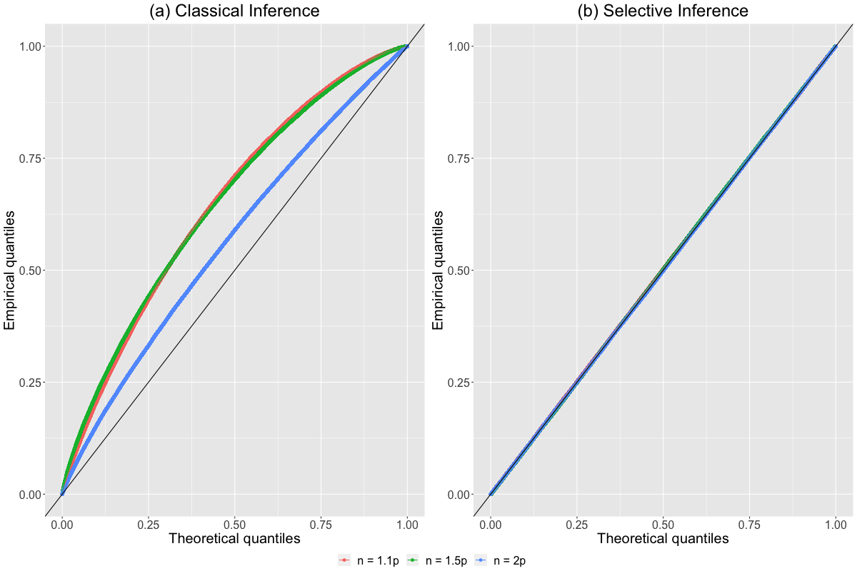
Figure 2: For 100,000 draws from (1), with $\bm{\Sigma}=\mathbf{I}_{100},n\in\left\{1.1p,1.5p,2p\right\}$, QQ-plots are displayed for: (a) the “classical” p-value in (6); (b) the “selective” p-value in (12), approximated as described in Section 4.

5.2 Power at $\alpha=0.05$

We simulate data with unordered variables from (1), with $p=100$, $n\in\left\{1.1p,1.5p,2p\right\}$. For each simulated data set, we generate a random $p\times p$ positive definite matrix $\Sigma$ and a corresponding threshold $c=c\left(\mbox{\boldmath$\Sigma$}\right)$ as described in Supplementary Material Section S8, and we randomly select $\hat{\mathcal{P}}\in\mathcal{P}\left(\textbf{S}\left(\textbf{x}\right)\right)$ with $\mathcal{P}\left(\cdot\right)$ defined in Section 3.1. We test $H_{0}^{\hat{\mathcal{P}}}:\mbox{\boldmath$\Sigma$}_{\hat{\mathcal{P}},\hat{\mathcal{P}}^{c}}=\mathbf{0}$ at significance level $\alpha=0.05$. Motivated by the test statistic in (3), we define the effect size based on its population counterpart as $\Delta:=1-\frac{\left|\mbox{\boldmath$\Sigma$}\right|}{\left|\mbox{\boldmath$\Sigma$}_{{\hat{\mathcal{P}}},{\hat{\mathcal{P}}}}\right|\left|\mbox{\boldmath$\Sigma$}_{{\hat{\mathcal{P}}^{c}},{\hat{\mathcal{P}}^{c}}}\right|}$, and consider the probability of rejecting $H_{0}^{\hat{\mathcal{P}}}:\mbox{\boldmath$\Sigma$}_{\hat{\mathcal{P}},\hat{\mathcal{P}}^{c}}=\mathbf{0}$ as a function of $\Delta$ over $1,000,000$ simulated data sets. Figure 3 shows that the proposed selective inference approach has higher power than classical inference for all values of $\Delta$ and $n$.

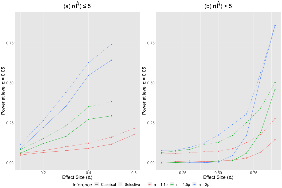
Figure 3: Power estimates as a function of the effect-size $\Delta$ for 1,000,000 draws from the simulation setup described in Section 5.2, when (a) $r\left(\hat{\mathcal{P}}\right)\leqslant 5$, (b) $r\left(\hat{\mathcal{P}}\right)>5$, where $r\left(\hat{\mathcal{P}}\right)=\min\left\{\mathrm{card}\left({\hat{\mathcal{P}}}\right),\mathrm{card}\left(\hat{\mathcal{P}}^{c}\right)\right\}$. The x-axis displays bins of $\Delta$ of size $0.1$; only bins with more than $100$ simulated datasets are displayed.

6 Application to gene co-expression networks

A gene co-expression network is an undirected graph in which the nodes represent genes and the edges represent pairs of genes that are co-expressed, in the sense of e.g. Pearson correlation (Guttman et al.,, 2011). Although gene co-expression networks do not confer information about causality, they are frequently used as a starting point for investigating gene regulation, functional enrichment, and hub genes (Van Dam et al.,, 2018). Additionally, they have proven useful in identifying disease genes through the guilt-by-association principle, enabling a better understanding of disease origin (Alsina et al.,, 2014) and progression (Chaussabel et al.,, 2008). For a detailed review of gene co-expression networks, we refer readers to Saelens et al., (2018) and references therein.

In this section, we focus on the gene expression data corresponding to E. coli and S. cerevisiae from the DREAM5 network inference challenge (Marbach et al.,, 2012). We will test for correlation between sets of genes that are known to be correlated based on outside biological knowledge. Our results indicate that our proposed selective inference approach has higher power than the classical inference approach.

6.1 Escherichia coli and Saccharomyces cerevisiae data sets

The DREAM5 E. coli data set consists of pre-processed gene expression measurements for $p=$ 4,297 genes on $n=$ 805 microarray chips (Marbach et al.,, 2012). Furthermore, the E. coli gene co-expression network is very well understood, and known edges can be found in publicly available databases, e.g. RegulonDB (Gama-Castro et al.,, 2010) and EcoCyc (Keseler et al.,, 2010). As part of the DREAM5 challenge, a highly curated co-expression network, based on this outside biological information, was made available. We treat this as a “ground truth” co-expression network in what follows.

The DREAM5 S. cerevisiae data set consists of $p=$ 5,667 pre-processed gene expression measurements on $n=$ 536 microarrays. While the S. cerevisiae network is not as well understood as the E. coli network, the DREAM5 organizers combined data from 16 sources to arrive at a single co-expression network (MacIsaac et al.,, 2006). We treat this network as the “ground truth” in what follows.

6.2 Power to detect correlation between sets of genes

For each data set, we identify the gene with the most edges in the ground truth co-expression network, and restrict our analysis to that hub gene and $99$ genes randomly sampled from the genes to which it is connected. This yields a set of $p=100$ genes that form a single connected component in the ground truth co-expression network. By construction, for any $\hat{\mathcal{P}}\in\left\{1,2,\ldots,p\right\}$, the null hypothesis $H_{0}^{\hat{\mathcal{P}}}:\mbox{\boldmath$\Sigma$}_{\hat{\mathcal{P}},\hat{\mathcal{P}}^{c}}=\mathbf{0}$ will not hold.

Next, we sample $n\in\left\{1.2p,1.4p,1.5p,2p\right\}$ microarrays, and let x denote the resulting $n\times p$ data set. We then compute $\mathcal{P}\left(\textbf{S}\left(\textbf{x}\right)\right)$ using the procedure in Section 3.1. To choose the threshold $c$, we apply the procedure described in Supplementary Material Section S8 to the sample covariance matrix computed on the held-out microarrays $\left(\text{which we write as }\hat{\textbf{S}}_{holdout}\right)$, i.e. those not included in x. Since the microarrays are independent, this threshold $c$ is independent of x. For a randomly selected $\hat{\mathcal{P}}\in\mathcal{P}\left(\textbf{S}\left(\textbf{x}\right)\right)$, we test $H_{0}^{\hat{\mathcal{P}}}:\mbox{\boldmath$\Sigma$}_{\hat{\mathcal{P}},\hat{\mathcal{P}}^{c}}=\mathbf{0}$ at significance level $\alpha=0.05$, where $\Sigma$ denotes the population covariance matrix of the $p$ genes. We repeat this entire procedure 10,000 times for different random sets of $99$ neighbors of the hub gene.

Figures 4(a) and 5(a) display the probability of rejecting $H_{0}^{\hat{\mathcal{P}}}:\mbox{\boldmath$\Sigma$}_{\hat{\mathcal{P}},\hat{\mathcal{P}}^{c}}=\mathbf{0}$ as a function of $\hat{\Delta}:=1-\frac{\left|\hat{\textbf{S}}_{holdout}\right|}{\left|\hat{\textbf{S}}_{{holdout}_{\hat{\mathcal{P}},\hat{\mathcal{P}}}}\right|\left|\hat{\textbf{S}}_{{holdout}_{\hat{\mathcal{P}}^{c},\hat{\mathcal{P}}^{c}}}\right|}$. In this setting, by construction, the $p=100$ genes have extremely high correlation. For any $\hat{\mathcal{P}}\in\mathcal{P}\left(\textbf{S}\left(\textbf{x}\right)\right)$, the conditioning set in (13) deals with a modified version $\textbf{S}^{\prime}\left(\textbf{x},\hat{\mathcal{P}},\cdot\right)$ of the sample covariance matrix $\textbf{S}\left(\textbf{x}\right)$ with a perturbed off-diagonal block (recall Theorem 1). Because the genes are highly correlated, for perturbations under $H_{0}^{\hat{\mathcal{P}}}$, with very high probability, we will have $\mathcal{P}\left(\textbf{S}^{\prime}\left(\textbf{x},\hat{\mathcal{P}},\cdot\right)\right)=\mathcal{P}\left(\textbf{S}\left(\textbf{x}\right)\right)$. Hence the classical and selective approaches yield almost identical results.

To investigate the performance of the classical and selective approaches when the correlation between genes is lower, we add Gaussian white noise to each gene’s expression, as follows:

$$\tilde{\mathbf{x}}_{j}=\mathbf{x}_{j}+\eta\bm{\varepsilon}_{j},\>\>\>\bm{\varepsilon}_{j}\sim N\left(\mathbf{0},\widehat{\mathrm{var}}\left(\mathbf{x}_{j}\right)\mathbf{I}\right),\>\>j=1,2,\ldots,p.$$ (23)

Here $\mathbf{x}_{j}\in\mathbb{R}^{n}$ is the expression vector for the $j^{th}$ gene, i.e. the $j^{th}$ column of x. We vary the noise level $\eta\in\left\{0.5,3\right\}$. In Figures 4 and 5, we see that the power of both the classical and selective approaches decreases as $\eta$ increases. Moreover, as $\eta$ increases, the correlation between the genes decreases. Hence for perturbations under $H_{0}^{\hat{\mathcal{P}}}$, the probability of the event $\mathcal{P}\left(\textbf{S}^{\prime}\left(\textbf{x},\hat{\mathcal{P}},\cdot\right)\right)=\mathcal{P}\left(\textbf{S}\left(\textbf{x}\right)\right)$ decreases. As a result, the difference between the classical and selective approaches increases, and the selective approach becomes more powerful than the classical approach.

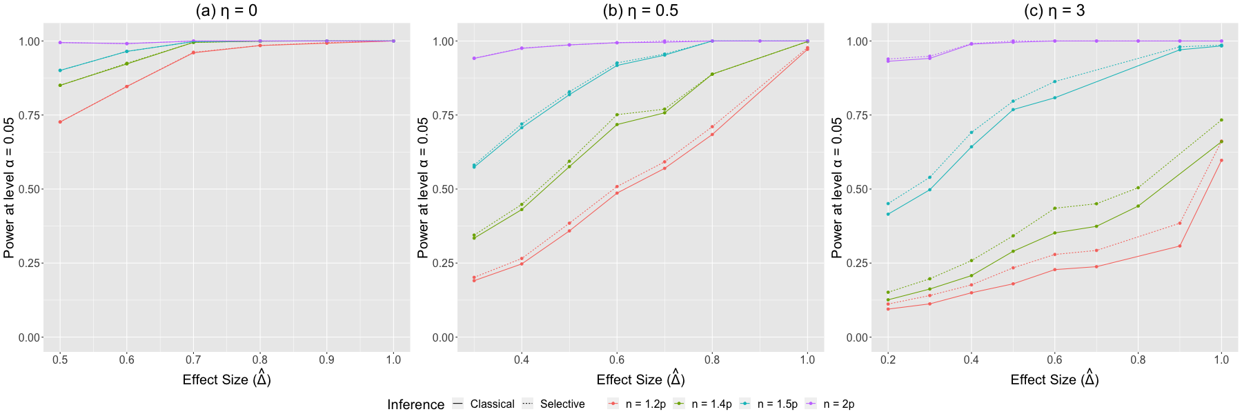
Figure 4: Power estimates as a function of $\hat{\Delta}$ for E. coli for three values of $\eta$ in (23). (a) $\eta=0$, (b) $\eta=0.5$, (c) $\eta=3$ in (23). We only display bins of $\hat{\Delta}$ with more than 100 observations.

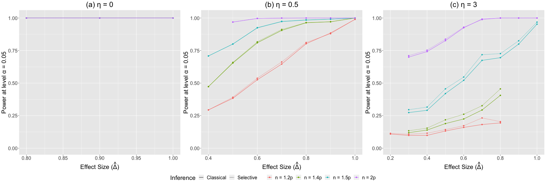
Figure 5: Power estimates as a function of $\hat{\Delta}$ for S. cerevisiae for three values of $\eta$ in (23). (a) $\eta=0$, (b) $\eta=0.5$, (c) $\eta=3$ in (23). We only display bins of $\hat{\Delta}$ with more than 100 observations.

7 Discussion

Our proposed approach for testing dependence between data-driven groups of Gaussian variables requires the number of features to be less than the number of observations, i.e. $p<n$, in order for the test statistic to be defined. Future work could combine tools from high-dimensional inference with selective inference to account for selection in covariance matrices with $p\gg n$.

The normality assumption on the variables is needed to obtain Proposition 1, but is restrictive in practice. For example, RNA sequencing data involve nonnegative counts, which are better modeled with a Poisson (Witten,, 2011) or negative binomial (Risso et al.,, 2018) distribution. Extending the proposed selective inference approach to accommodate a more general class of distributions requires further investigation.

An R package to implement the proposed approach called independencepvalue is available at https://arkajyotisaha.github.io/independencepvalue-project.

Supplementary Materials for “Inferring independent sets of Gaussian variables after thresholding correlations"

S1 Brief review of canonical correlation analysis

Here we briefly review canonical correlation analysis, as it paves the way for the selective inference method proposed in this paper. We largely follow the notation used in Anderson, (2003).

We partition the random vector $X\sim N\left(0,\bm{\Sigma}\right)$ of length $p$ into two vectors $X_{1}$ and $X_{2}$ of lengths $p_{1}$ and $p_{2}=p-p_{1}$ respectively, so that $X^{\top}=\left(X_{1}^{\top}\>\>\>X_{2}^{\top}\right)$. The corresponding covariance matrix can be partitioned as

$$\mbox{\boldmath$\Sigma$}=\begin{pmatrix}\mbox{\boldmath$\Sigma$}_{11}&\mbox{\boldmath$\Sigma$}_{12}\\ \mbox{\boldmath$\Sigma$}_{21}&\mbox{\boldmath$\Sigma$}_{22}\end{pmatrix},$$

where $\bm{\Sigma}$ is of dimension $p\times p$, $\bm{\Sigma}_{12}$ is of dimension $p_{1}\times p_{2}$, etc. Without loss of generality, we assume $p_{1}\leqslant p_{2}$. We define the population canonical correlations $\lambda_{1},\lambda_{2},\ldots,\lambda_{p_{1}}$ between $X_{1}$ and $X_{2}$, and their corresponding population canonical vectors $\textbf{A}^{*}=\left(\alpha_{1}^{*},\alpha_{2}^{*},\ldots,\alpha_{p_{1}}^{*}\right)\in\mathbb{R}^{p_{1}\times p_{1}}$ and $\bm{\Gamma}^{*}=\left(\gamma_{1}^{*},\gamma_{2}^{*},\ldots,\gamma_{p_{1}}^{*}\right)\in\mathbb{R}^{p_{2}\times p_{1}}$, sequentially for $r=1,2,\ldots,p_{1}$:

$$\left(\bm{\alpha}_{r}^{*},\bm{\gamma}_{r}^{*}\right):= \operatorname*{arg\,max}_{\begin{subarray}{c}\bm{\alpha}_{r}^{\top}\bm{\Sigma}_{11}\bm{\alpha}_{r}=1\\ \bm{\gamma}_{r}^{\top}\bm{\Sigma}_{22}\bm{\gamma}_{r}=1\\ \bm{\alpha}_{r}^{\top}\bm{\Sigma}_{11}\bm{\alpha}_{j}^{*}=0;\forall j<r\\ \bm{\gamma}_{r}^{\top}\bm{\Sigma}_{22}\bm{\gamma}_{j}^{*}=0;\forall j<r\end{subarray}}\bm{\alpha}_{r}^{\top}\bm{\Sigma}_{12}\bm{\gamma}_{r};\>\>\>\>\>\>\>\>\>\>\>\>\>\lambda_{r}:=\left(\bm{\alpha}_{r}^{*}\right)^{\top}\bm{\Sigma}_{12}\bm{\gamma}_{r}^{*}.$$ (S1a)

The above can be solved through an SVD on $$\mbox{\boldmath$\Sigma$}_{11}^{-\frac{1}{2}}\mbox{\boldmath$\Sigma$}_{12}\mbox{\boldmath$\Sigma$}_{22}^{-\frac{1}{2}}=\mathbf{A}\bm{\Lambda}\bm{\Gamma}^{\top} \mathbf{A}^{*}=\mbox{\boldmath$\Sigma$}_{11}^{-\frac{1}{2}}\mathbf{A},\bm{\Gamma}^{*}=\mbox{\boldmath$\Sigma$}_{22}^{-\frac{1}{2}}\bm{\Gamma} \bm{\lambda}_{r}=\mathrm{diag}\left(\bm{\Lambda}\right) \textbf{x}\in\mathbb{R}^{n\times p} \mathrm{rank}\left(\textbf{x}\right)=p 1 \bm{\Sigma} \textbf{S}=\begin{pmatrix}\textbf{S}_{11}&\textbf{S}_{12}\\ \textbf{S}_{12}^{\top}&\textbf{S}_{22}\end{pmatrix} \textbf{x}=\left(\textbf{x}_{1}^{\top}\>\>\>\textbf{x}_{2}^{\top}\right)^{\top} \textbf{x}_{1} \textbf{x}_{2} {\textbf{x}}^{W}_{1}=\textbf{S}_{11}^{-\frac{1}{2}}\textbf{x}_{1} {\textbf{x}}^{W}_{2}=\textbf{S}_{22}^{-\frac{1}{2}}\textbf{x}_{2}. \mathbf{S}^{W}=\begin{pmatrix}\mathbf{S}^{W}_{11}&\mathbf{S}^{W}_{12}\\ \left(\mathbf{S}^{W}_{12}\right)^{\top}&\mathbf{S}^{W}_{22}\end{pmatrix} {\textbf{x}}^{W}=\left(\left({\textbf{x}}^{W}_{1}\right)^{\top}\>\>\>\left({\textbf{x}}^{W}_{2}\right)^{\top}\right)^{\top} \mathbf{S}^{W}_{11}=\textbf{I}_{p_{1}};\>\mathbf{S}^{W}_{22}=\textbf{I}_{p_{2}},\text{ and }\mathbf{S}^{W}_{12}=\textbf{S}_{11}^{-\frac{1}{2}}\textbf{S}_{12}\textbf{S}_{22}^{-\frac{1}{2}} \mathbf{S}^{W}_{12}$$, by taking , and (Jendoubi and Strimmer,, 2019). Next, we define the sample canonical correlations and sample canonical vectors for a realization of X in (1). We assume , which holds with probability , since we assume is positive definite. We let denote the sample covariance of , suitably partitioned. We now define the “whitened” versions of and , i.e. and Let denote the sample covariance matrix of , suitably partitioned. It follows that . The compact SVD of is

$$\mathbf{S}^{W}_{12}\overset{SVD}{=}\hat{\textbf{A}}\>\hat{\bm{\Lambda}}\>\hat{\bm{\Gamma}}^{\top},$$ (S1b)

where $\hat{\bm{\Lambda}}$ is a square diagonal matrix of $p_{1}$ positive singular values, arranged in non-increasing order, and $\hat{\textbf{A}}$ and $\hat{\bm{\Gamma}}$ are the $p_{1}\times p_{1}$ and $p_{2}\times p_{1}$ matrices of left and right singular vectors, respectively. We now derive (5). We can rewrite the classical LRT statistic in (3) by noting that

$$\left|\textbf{S}\right| =\left|\textbf{S}_{22}\right|\left|\textbf{S}_{11}-\textbf{S}_{12}\textbf{S}_{22}^{-1}\textbf{S}_{21}\right|$$

$$=\left|\textbf{S}_{22}\right|\left|\textbf{S}_{11}\right|\left|\textbf{I}-\textbf{S}_{11}^{-\frac{1}{2}}\textbf{S}_{12}\textbf{S}_{22}^{-\frac{1}{2}}\textbf{S}_{22}^{-\frac{1}{2}}\textbf{S}_{21}\textbf{S}_{11}^{-\frac{1}{2}}\right|$$

$$=\left|\textbf{S}_{11}\right|\left|\textbf{S}_{22}\right|\left|\textbf{I}-\mathbf{S}^{W}_{12}\left(\mathbf{S}^{W}_{12}\right)^{\top}\right|$$

$$=\left|\textbf{S}_{11}\right|\left|\textbf{S}_{22}\right|\left|\textbf{I}-\hat{\bm{\Lambda}}^{2}\right|,$$

where in the last equality, we have used that $\hat{\mathbf{A}}$ is a square orthogonal matrix.

S2 Proof of Proposition 1

For any subset $\mathcal{P}$ of $\{1,2,\ldots,p\}$, the sample canonical correlations are the diagonal elements of $\hat{\bm{\Lambda}}^{\mathcal{P}}$, denoted by $\left\{\hat{\lambda}_{i}^{\mathcal{P}}\right\}_{i=1}^{r\left({\mathcal{P}}\right)}$. In this section, we will omit the ${\mathcal{P}}$ superscript and write $\left\{\hat{\lambda}_{i}\right\}_{i=1}^{r\left({\mathcal{P}}\right)}$.

S2.1 Proof of Proposition 1(i)

Proof.

The joint density of $\left(\hat{\lambda}_{1}^{2},\hat{\lambda}_{2}^{2},\ldots,\hat{\lambda}_{r\left(\mathcal{P}\right)}^{2}\right)$ under $H_{0}^{\mathcal{P}}$ takes the form

$$f\left(\hat{\lambda}_{1}^{2}=\gamma_{1},\hat{\lambda}_{2}^{2}=\gamma_{2},\ldots,\hat{\lambda}_{r\left(\mathcal{P}\right)}^{2}=\gamma_{r\left(\mathcal{P}\right)}\right)= \pi^{\frac{1}{2}\left(r\left(\mathcal{P}\right)\right)^{2}}\frac{\Gamma_{r\left(\mathcal{P}\right)}\left(\frac{n}{2}\right)}{\Gamma_{r\left(\mathcal{P}\right)}\left(\frac{n-p+r\left(\mathcal{P}\right)}{2}\right)\Gamma_{p}\left(\frac{1}{2}r\left(\mathcal{P}\right)\right)\Gamma_{p}\left(\frac{1}{2}\left(p-r\left(\mathcal{P}\right)\right)\right)}\times$$ (S2)

$$\prod_{i=1}^{r\left(\mathcal{P}\right)}\left\{\gamma_{i}^{\frac{1}{2}\left(\left|p-2\mathrm{card}\left({\mathcal{P}}\right)\right|-1\right)}\left(1-\gamma_{i}\right)^{\frac{1}{2}\left(n-p-2\right)}\right\}\prod_{i<j}\left(\gamma_{i}-\gamma_{j}\right)$$

by (13) in Section 13.4 in Anderson, (2003). To obtain $f\left(\hat{\lambda}_{1},\hat{\lambda}_{2},\ldots,\hat{\lambda}_{r\left(\mathcal{P}\right)}\right)$ in (7), we perform a change of variables. We have

$$f\left(\hat{\lambda}_{1},\hat{\lambda}_{2},\ldots,\hat{\lambda}_{r\left(\mathcal{P}\right)}\right)=f\left(\hat{\lambda}_{1}^{2},\hat{\lambda}_{2}^{2},\ldots,\hat{\lambda}_{r\left(\mathcal{P}\right)}^{2}\right)\left|\mathbf{J}\right|,$$ (S3)

where $\mathbf{J}$ is the $r\left(\mathcal{P}\right)\times r\left(\mathcal{P}\right)$ Jacobian matrix of the transformation, with $\mathbf{J}_{i,j}=\frac{\partial\hat{\lambda}_{i}^{2}}{\partial\hat{\lambda}_{j}}$ for $i,j\in\left\{1,2,\ldots,r\left(\mathcal{P}\right)\right\}$. Simplifying, we have $\left|\mathbf{J}\right|=2^{r\left(\mathcal{P}\right)}\prod_{i=1}^{r\left(\mathcal{P}\right)}\hat{\lambda}_{i}$. Substituting this into (S3) yields

$$f\left(\hat{\lambda}_{1},\hat{\lambda}_{2},\ldots,\hat{\lambda}_{r\left(\mathcal{P}\right)}\right)= \pi^{\frac{1}{2}\left(r\left(\mathcal{P}\right)\right)^{2}}\frac{\Gamma_{r\left(\mathcal{P}\right)}\left(\frac{n}{2}\right)}{\Gamma_{r\left(\mathcal{P}\right)}\left(\frac{n-p+r\left(\mathcal{P}\right)}{2}\right)\Gamma_{p}\left(\frac{1}{2}r\left(\mathcal{P}\right)\right)\Gamma_{p}\left(\frac{1}{2}\left(p-r\left(\mathcal{P}\right)\right)\right)}\times$$ (S4)

$$\prod_{i=1}^{r\left(\mathcal{P}\right)}\left\{\hat{\lambda}_{i}^{\left(\left|p-2\mathrm{card}\left({\mathcal{P}}\right)\right|-1\right)}\left(1-\hat{\lambda}_{i}^{2}\right)^{\frac{1}{2}\left(n-p-2\right)}\right\}\prod_{i<j}\left(\hat{\lambda}_{i}^{2}-\hat{\lambda}_{j}^{2}\right)\times 2^{r\left(\mathcal{P}\right)}\prod_{i=1}^{r\left(\mathcal{P}\right)}\hat{\lambda}_{i},$$

which completes the proof of (i) of Proposition 1. ∎

S2.2 Proof of Proposition 1(ii)

Proof.

The result follows by applying various arguments from Anderson, (2003). For clarity, we extract the relevant parts here. For notational ease, we will write $\mathbf{S}\left(\textbf{x}\right)$ as $\mathbf{S}$.

1. Applying the argument in (48)-(52) of Section 12.2 of Anderson, (2003) to the sample covariance matrix, we have that the squared canonical correlations $\left\{\hat{\lambda}_{i}^{2}\right\}_{i=1}^{r\left({\mathcal{P}}\right)}$ are the roots, with respect to $\gamma$, of

   $$f\left(\gamma\right)=\left|\textbf{S}_{{\mathcal{P}},{\mathcal{P}}^{c}}\left(\textbf{S}_{{\mathcal{P}}^{c},{\mathcal{P}}^{c}}\right)^{-1}\textbf{S}_{{\mathcal{P}}^{c},{\mathcal{P}}}-\gamma\textbf{S}_{{\mathcal{P}},{\mathcal{P}}}\right|.$$ (S5)

2. By Corollary 4.3.2 of Anderson, (2003), if $\mbox{\boldmath$\Sigma$}_{{\mathcal{P}},{\mathcal{P}}^{c}}=0$, then

   W $$:=n\left(\mbox{\boldmath$\Sigma$}_{{\mathcal{P}},{\mathcal{P}}}\right)^{-\frac{1}{2}}\textbf{S}_{{\mathcal{P}},{\mathcal{P}}^{c}}\left(\textbf{S}_{{\mathcal{P}}^{c},{\mathcal{P}}^{c}}\right)^{-1}\textbf{S}_{{\mathcal{P}}^{c},{\mathcal{P}}}\left(\mbox{\boldmath$\Sigma$}_{{\mathcal{P}},{\mathcal{P}}}\right)^{-\frac{1}{2}}\sim\mathrm{Wishart}_{r\left({\mathcal{P}}\right)}\left(\textbf{I},p-r\left({\mathcal{P}}\right)\right),$$

   T $$:=n\left(\mbox{\boldmath$\Sigma$}_{{\mathcal{P}},{\mathcal{P}}}\right)^{-\frac{1}{2}}\left(\textbf{S}_{{\mathcal{P}},{\mathcal{P}}}-\textbf{S}_{{\mathcal{P}},{\mathcal{P}}^{c}}\left(\textbf{S}_{{\mathcal{P}}^{c},{\mathcal{P}}^{c}}\right)^{-1}\textbf{S}_{{\mathcal{P}}^{c},{\mathcal{P}}}\right)\left(\mbox{\boldmath$\Sigma$}_{{\mathcal{P}},{\mathcal{P}}}\right)^{-\frac{1}{2}}\sim\mathrm{Wishart}_{r\left({\mathcal{P}}\right)}\left(\textbf{I},n-1-p+r\left({\mathcal{P}}\right)\right),$$

   and W and T are independent.

3. Equations 7-10 of Section 13.2 of Anderson, (2003) establish that the values of $\gamma$ that satisfy $\left|\textbf{W}-\gamma\left(\textbf{T}+\textbf{W}\right)\right|=0$ are given by $\frac{\Psi_{i}\left(\textbf{W}\textbf{T}^{-1}\right)}{1+\Psi_{i}\left(\textbf{W}\textbf{T}^{-1}\right)}$, where $\Psi_{i}\left(\textbf{W}\textbf{T}^{-1}\right)$ are the eigenvalues of $\textbf{W}\textbf{T}^{-1}$.

By 1), $\hat{\lambda}_{1}^{2},\hat{\lambda}_{2}^{2},\ldots,\hat{\lambda}_{r\left(\mathcal{P}\right)}^{2}$ are given by roots of (S5). Pre- and post-multiplying
$\textbf{S}_{{\mathcal{P}},{\mathcal{P}}^{c}}\left(\textbf{S}_{{\mathcal{P}}^{c},{\mathcal{P}}^{c}}\right)^{-1}\textbf{S}_{{\mathcal{P}}^{c},{\mathcal{P}}}-\gamma\textbf{S}_{{\mathcal{P}},{\mathcal{P}}}$ in (S5) by $\sqrt{n}\mbox{\boldmath$\Sigma$}_{{\mathcal{P}},{\mathcal{P}}}^{-\frac{1}{2}}$ gives that $\hat{\lambda}_{1}^{2},\hat{\lambda}_{2}^{2},\ldots,\hat{\lambda}_{r\left(\mathcal{P}\right)}^{2}$ are the values of $\gamma$ that solve

$$\left|\textbf{W}-\gamma\left(\textbf{T}+\textbf{W}\right)\right|=0,$$

where W and T are defined in 2). Applying 3) completes the proof of (ii) of Proposition 1. ∎

S2.3 Proof of Proposition 1(iii)

Proof.

To prove Proposition 1(iii), we start with a result whose proof follows from (5) in Section 4.4.1 of Anderson, (2003).

Proposition 5.

The squared sample multiple correlation coefficient for regression for a response $\mathbf{h}$ on a set of variables $\mathcal{Q}$ is given by $\frac{\mathbf{s}_{\mathcal{Q},\mathbf{h}}^{\top}\left(\mathbf{S}_{\mathcal{Q},\mathcal{Q}}\right)^{-1}\mathbf{s}_{\mathcal{Q},\mathbf{h}}}{\mathrm{var}\left(\mathbf{h}\right)}$, where $s_{\mathcal{Q},\mathbf{h}}$ denotes the vector of covariances between $\mathbf{h}$ and the variables in $\mathcal{Q}$, and $\mathbf{S}_{\mathcal{Q},\mathcal{Q}}$ denotes the covariance matrix of the variables in $\mathcal{Q}$.

Without loss of generality, we assume $\mathrm{card}\left({\mathcal{P}}\right)=p-1$. First we establish that the canonical correlation is the multiple correlation coefficient between the variable in ${\mathcal{P}}^{c}$ and the remaining $p-1$ variables in ${\mathcal{P}}$. We write $\mathbf{S}\left(\textbf{x}\right)$ as $\mathbf{S}$ and denote the vectors $\mathbf{S}^{W}_{{\mathcal{P}},{\mathcal{P}}^{c}}$ and $\textbf{S}_{{\mathcal{P}},{\mathcal{P}}^{c}}$ as $\mathbf{s}^{W}_{{\mathcal{P}},{\mathcal{P}}^{c}}$ and $\textbf{s}_{{\mathcal{P}},{\mathcal{P}}^{c}}$, respectively, and the scalar $\textbf{S}_{{\mathcal{P}}^{c},{\mathcal{P}}^{c}}$ as $s_{{\mathcal{P}}^{c},{\mathcal{P}}^{c}}$. Substituting these in (4) we have

$$\mathbf{s}^{W}_{{\mathcal{P}},{\mathcal{P}}^{c}}=\frac{\left(\textbf{S}_{{{\mathcal{P}}},{{\mathcal{P}}}}\right)^{-\frac{1}{2}}\textbf{s}_{{\mathcal{P}},{\mathcal{P}}^{c}}}{\sqrt{s_{{\mathcal{P}}^{c},{\mathcal{P}}^{c}}}}.$$

Moreover, $\hat{\bm{\Lambda}}^{{\mathcal{P}}}$ is a scalar, which we denote as $\hat{\lambda}_{1}$. From (4), $\hat{\lambda}_{1}$ is precisely the singular value of the vector $\mathbf{s}^{W}_{{\mathcal{P}},{\mathcal{P}}^{c}}$, which is $\left\|\mathbf{s}^{W}_{{\mathcal{P}},{\mathcal{P}}^{c}}\right\|_{2}$. Hence we have

$$\left(\hat{\lambda}_{1}\right)^{2}=\|\mathbf{s}^{W}_{{\mathcal{P}},{\mathcal{P}}^{c}}\|_{2}^{2}=\left(\mathbf{s}^{W}_{{\mathcal{P}},{\mathcal{P}}^{c}}\right)^{\top}\mathbf{s}^{W}_{{\mathcal{P}},{\mathcal{P}}^{c}}=\frac{\textbf{s}_{{\mathcal{P}},{\mathcal{P}}^{c}}^{\top}\left(\textbf{S}_{{{\mathcal{P}}},{{\mathcal{P}}}}\right)^{-1}\textbf{s}_{{\mathcal{P}},{\mathcal{P}}^{c}}}{s_{{\mathcal{P}}^{c},{\mathcal{P}}^{c}}}.$$

Using Proposition 5, $\frac{\textbf{s}_{{\mathcal{P}},{\mathcal{P}}^{c}}^{\top}\left(\textbf{S}_{{{\mathcal{P}}},{{\mathcal{P}}}}\right)^{-1}\textbf{s}_{{\mathcal{P}},{\mathcal{P}}^{c}}}{s_{{\mathcal{P}}^{c},{\mathcal{P}}^{c}}}$ is the squared multiple correlation coefficient for the regression of the single variable in ${\mathcal{P}}^{c}$ onto the remaining $p-1$ variables. Under the null, the squared sample multiple correlation coefficient follows a beta distribution with parameters $\frac{p-1}{2}$ and $\frac{n-p}{2}$ (Ali and Nagar,, 2002). This completes the proof of (iii) of Proposition 1. ∎

S3 Proof of Theorem 1

In this section, we abbreviate $H_{0}^{{\mathcal{R}}},\hat{\mathbf{A}}^{{\mathcal{R}}}\left(\cdot\right),\hat{\bm{\Lambda}}^{{\mathcal{R}}}\left(\cdot\right)$, and $\hat{\mathbf{\Gamma}}^{{\mathcal{R}}}\left(\cdot\right)$ (defined in Section 2) by omitting the superscript. Without loss of generality, we assume that $\mathcal{R}=\left\{1,2,\ldots,p_{1}\right\}$, $\mathcal{R}^{c}=\left\{p_{1}+1,\ldots,p\right\}$, and $p_{1}\leqslant p/2$. Define $p_{2}=p-p_{1}$. Let $\hat{\lambda}_{1}\left(\textbf{X}\right),\hat{\lambda}_{2}\left(\textbf{X}\right),\ldots,\hat{\lambda}_{p_{1}}\left(\textbf{X}\right)$ be the diagonal elements of $\hat{\bm{\Lambda}}\left(\textbf{X}\right)$.

We let $\textbf{S}\left(\textbf{X}\right)=\begin{pmatrix}\textbf{S}_{11}\left(\textbf{X}\right)&\textbf{S}_{12}\left(\textbf{X}\right)\\ \textbf{S}_{12}^{\top}\left(\textbf{X}\right)&\textbf{S}_{22}\left(\textbf{X}\right)\end{pmatrix}$ denote the covariance matrix of $\textbf{X}=\left(\textbf{X}_{1}\>\>\>\textbf{X}_{2}\right)$, suitably partitioned, where $\textbf{X}_{1}$ and $\textbf{X}_{2}$ are defined as the submatrices of X with columns in $\mathcal{R}$ and ${\mathcal{R}}^{c}$, respectively. Equipped with this notation, we first state a technical lemma whose proof we defer to Section S3.1.

Lemma S3.1.

Under $H_{0}:\bm{\Lambda}=\mathbf{0}$, $\hat{\bm{\Lambda}}\left(\mathbf{X}\right)$ is independent of $\left(\mathbf{S}_{11}\left(\mathbf{X}\right),\mathbf{S}_{22}\left(\mathbf{X}\right),\hat{\mathbf{A}}\left(\mathbf{X}\right),\hat{\bm{\Gamma}}\left(\mathbf{X}\right)\right)$.

By (4), $\hat{\mathbf{A}}\left(\mathbf{X}\right)\hat{\bm{\Lambda}}\left(\textbf{X}\right)\left(\hat{\mathbf{\Gamma}}\left(\mathbf{X}\right)\right)^{\top}$ is the SVD of $\left(\mathbf{S}_{11}\left(\mathbf{X}\right)\right)^{-\frac{1}{2}}\textbf{S}_{12}\left(\textbf{X}\right)\left(\mathbf{S}_{22}\left(\mathbf{X}\right)\right)^{-\frac{1}{2}}$ and so
$\textbf{S}_{12}\left(\textbf{X}\right)=\left(\mathbf{S}_{11}\left(\mathbf{X}\right)\right)^{\frac{1}{2}}\hat{\mathbf{A}}\left(\mathbf{X}\right)\hat{\bm{\Lambda}}\left(\textbf{X}\right)\left(\hat{\mathbf{\Gamma}}\left(\mathbf{X}\right)\right)^{\top}\left(\mathbf{S}_{22}\left(\mathbf{X}\right)\right)^{\frac{1}{2}}$. In (12), we condition on the additional information

$$\left\{\textbf{S}_{11}\left(\textbf{X}\right)=\textbf{S}_{11}\left(\textbf{x}\right),\textbf{S}_{22}\left(\textbf{X}\right)=\textbf{S}_{22}\left(\textbf{x}\right),\hat{\textbf{A}}\left(\textbf{X}\right)=\hat{\textbf{A}}\left(\textbf{x}\right),\hat{\bm{\Gamma}}\left(\textbf{X}\right)=\hat{\bm{\Gamma}}\left(\textbf{x}\right)\right\}.$$ (S6)

On this conditioning set, we have that $\mathbf{S}_{12}\left(\mathbf{X}\right)=\left(\mathbf{S}_{11}\left(\mathbf{x}\right)\right)^{\frac{1}{2}}\hat{\mathbf{A}}\left(\mathbf{x}\right)\hat{\bm{\Lambda}}\left(\textbf{X}\right)\left(\hat{\mathbf{\Gamma}}\left(\mathbf{x}\right)\right)^{\top}\left(\mathbf{S}_{22}\left(\mathbf{x}\right)\right)^{\frac{1}{2}}$. Recalling the definition in (15), we see that $\mathbf{S}_{12}\left(\mathbf{X}\right)=\textbf{S}_{12}^{\prime}\left(\mathbf{x},\mathcal{R},\left\{\hat{\lambda}_{i}\left(\textbf{X}\right)\right\}_{i=1}^{p_{1}}\right)$. Thus, on the conditioning set (S6), we have that

$$\textbf{S}\left(\textbf{X}\right) =\begin{pmatrix}\mathbf{S}_{11}\left(\mathbf{x}\right)&\mathbf{S}_{12}^{\prime}\left(\mathbf{x},\mathcal{R},\left\{\hat{\lambda}_{i}\left(\textbf{X}\right)\right\}_{i=1}^{p_{1}}\right)\\ \left(\mathbf{S}_{12}^{\prime}\left(\mathbf{x},\mathcal{R},\left\{\hat{\lambda}_{i}\left(\textbf{X}\right)\right\}_{i=1}^{p_{1}}\right)\right)^{\top}&\mathbf{S}_{22}\left(\mathbf{x}\right)\end{pmatrix}=\mathbf{S}^{\prime}\left(\mathbf{x},\mathcal{R},\left\{\hat{\lambda}_{i}\left(\textbf{X}\right)\right\}_{i=1}^{p_{1}}\right),$$

where $\mathbf{S}^{\prime}\left(\mathbf{x},\mathcal{R},\left\{\hat{\lambda}_{i}\left(\textbf{X}\right)\right\}_{i=1}^{p_{1}}\right)$ was defined in Theorem 1. Therefore, we can rewrite $p\left(\mathbf{x};\mathcal{R}\right)$ in (12) as

$$p\left(\mathbf{x};\mathcal{R}\right)=\mathbb{P}_{H_{0}}\bigg{(}\prod_{i=1}^{p_{1}}\left(1-\left(\hat{\lambda}_{i}\left(\textbf{X}\right)\right)^{2}\right)\leqslant\prod_{i=1}^{p_{1}}\left(1-\left(\hat{\lambda}_{i}\left(\textbf{x}\right)\right)^{2}\right)\bigg{|} \mathcal{R}\in\mathcal{P}\left(\textbf{S}^{\prime}\left(\textbf{x},\mathcal{R},\left\{\lambda_{i}\left(\textbf{X}\right)\right\}_{i=1}^{p_{1}}\right)\right),$$

$$\textbf{S}_{11}\left(\textbf{X}\right)=\textbf{S}_{11}\left(\textbf{x}\right),\textbf{S}_{22}\left(\textbf{X}\right)=\textbf{S}_{22}\left(\textbf{x}\right),$$

$$\hat{\textbf{A}}\left(\textbf{X}\right)=\hat{\textbf{A}}\left(\textbf{x}\right),\hat{\bm{\Gamma}}\left(\textbf{X}\right)=\hat{\bm{\Gamma}}\left(\textbf{x}\right)\bigg{)}.$$

From Lemma S3.1 we have that under $H_{0}$, $\left\{\hat{\lambda}_{i}\left(\textbf{X}\right)\right\}_{i=1}^{p_{1}}$ is independent of
$\left(\textbf{S}_{11}\left(\textbf{X}\right),\textbf{S}_{22}\left(\textbf{X}\right),\hat{\textbf{A}}\left(\textbf{X}\right),\hat{\bm{\Gamma}}\left(\textbf{X}\right)\right)$. It follows that

$$p\left(\mathbf{x};\mathcal{R}\right)=\mathbb{P}_{H_{0}}\bigg{(}\prod_{i=1}^{p_{1}}\left(1-\left(\hat{\lambda}_{i}\left(\textbf{X}\right)\right)^{2}\right)\leqslant\prod_{i=1}^{p_{1}}\left(1-\left(\hat{\lambda}_{i}\left(\textbf{x}\right)\right)^{2}\right)\bigg{|} \mathcal{R}\in\mathcal{P}\left(\textbf{S}^{\prime}\left(\textbf{x},\mathcal{R},\left\{\hat{\lambda}_{i}\left(\textbf{X}\right)\right\}_{i=1}^{p_{1}}\right)\right)\bigg{)}.$$

Recall from Proposition 1 that under $H_{0}$, $\left(\hat{\lambda}_{1}\left(\textbf{X}\right),\hat{\lambda}_{2}\left(\textbf{X}\right),\ldots,\hat{\lambda}_{p_{1}}\left(\textbf{X}\right)\right)$ has the density given in (7). Therefore, for $\left(\lambda_{1},\lambda_{2},\ldots,\lambda_{r\left(\mathcal{P}\right)}\right)$ with density given in (7), the first statement in Theorem 1 is established.

The proof of (16) is similar to the proof of Equation 11 in Theorem 1 of Gao et al., (2022). Using the probability integral transform we have that $p\left(\mathbf{x};\mathcal{R}\right)$ in (12) controls the selective type I error, i.e.

$$\mathbb{P}_{H_{0}}\bigg{(}p\left(\mathbf{X};\mathcal{R}\right)\leqslant\alpha\bigg{|}\mathcal{R}\in\mathcal{P}\left(\textbf{S}\left(\textbf{X}\right)\right) ,\textbf{S}_{11}\left(\textbf{X}\right)=\textbf{S}_{11}\left(\textbf{x}\right),\textbf{S}_{22}\left(\textbf{X}\right)=\textbf{S}_{22}\left(\textbf{x}\right),$$

$$\>\hat{\textbf{A}}\left(\textbf{X}\right)=\hat{\textbf{A}}\left(\textbf{x}\right),\hat{\bm{\Gamma}}\left(\textbf{X}\right)=\hat{\bm{\Gamma}}\left(\textbf{x}\right)\bigg{)}\leqslant\alpha.$$

By the law of iterated expectation,

$$\mathbb{P}_{H_{0}}\left(p\left(\mathbf{X};{\mathcal{R}}\right)\leqslant\alpha\bigg{|}{\mathcal{R}}\in\mathcal{P}\left(\textbf{S}\left(\textbf{X}\right)\right)\right)$$

$$=\mathbb{E}_{H_{0}}\left(\mathds{1}\left\{p\left(\mathbf{X};{\mathcal{R}}\right)\leqslant\alpha\right\}\bigg{|}{\mathcal{R}}\in\mathcal{P}\left(\textbf{S}\left(\textbf{X}\right)\right)\right)$$

$$=\mathbb{E}_{H_{0}}\bigg{(}\mathbb{E}_{H_{0}}\bigg{[}\mathds{1}\left\{p\left(\mathbf{X};{\mathcal{R}}\right)\leqslant\alpha\right\}\bigg{|}{\mathcal{R}}\in\mathcal{P}\left(\textbf{S}\left(\textbf{X}\right)\right),\textbf{S}_{11}\left(\textbf{X}\right)=\textbf{S}_{11}\left(\textbf{x}\right),\textbf{S}_{22}\left(\textbf{X}\right)=\textbf{S}_{22}\left(\textbf{x}\right),$$

$$\>\>\>\>\>\>\>\>\>\>\>\>\>\>\>\>\>\>\>\>\>\>\>\>\>\>\>\>\>\>\>\>\>\>\>\>\>\>\>\>\>\>\>\>\>\>\>\>\>\>\>\>\>\>\>\>\>\>\>\>\>\>\>\hat{\textbf{A}}\left(\textbf{X}\right)=\hat{\textbf{A}}\left(\textbf{x}\right),\hat{\bm{\Gamma}}\left(\textbf{X}\right)=\hat{\bm{\Gamma}}\left(\textbf{x}\right)\bigg{]}\bigg{|}{\mathcal{R}}\in\mathcal{P}\left(\textbf{S}\left(\textbf{X}\right)\right)\bigg{)}$$

$$\leqslant\mathbb{E}_{H_{0}}\left(\alpha\bigg{|}{\mathcal{R}}\in\mathcal{P}\left(\textbf{S}\left(\textbf{X}\right)\right)\right)$$

$$=\alpha.$$

This proves (16) and completes the proof of Theorem 1.

S3.1 Proof of Lemma S3.1

Proof.

In what follows, we omit the dependence of $\hat{\bm{\Lambda}}\left(\mathbf{X}\right),\mathbf{S}_{11}\left(\mathbf{X}\right),\mathbf{S}_{22}\left(\mathbf{X}\right),\hat{\mathbf{A}}\left(\mathbf{X}\right),\hat{\bm{\Gamma}}\left(\mathbf{X}\right)$ on X. Recall that (4) can be written as $\mathbf{S}^{W}_{12}=\textbf{S}_{11}^{-\frac{1}{2}}\textbf{S}_{12}\textbf{S}_{22}^{-\frac{1}{2}}\overset{SVD}{=}\hat{\textbf{A}}\hat{\bm{\Lambda}}\hat{\bm{\Gamma}}^{\top}$. We first prove a technical lemma that will help us in establishing Lemma S3.1 going forward.

Lemma S3.2.

Under $H_{0}:{\bm{\Lambda}}=\mathbf{0}$, $\hat{\bm{\Lambda}}$ and $\left(\mathbf{S}_{11},\hat{\mathbf{A}},\hat{\bm{\Gamma}}\right)$ are conditionally independent given $\mathbf{X}_{2}$, i.e. $\hat{\bm{\Lambda}}\mathchoice{\mathrel{\hbox to0.0pt{$\displaystyle\perp$\hss}\mkern 2.0mu{\displaystyle\perp}}}{\mathrel{\hbox to0.0pt{$\textstyle\perp$\hss}\mkern 2.0mu{\textstyle\perp}}}{\mathrel{\hbox to0.0pt{$\scriptstyle\perp$\hss}\mkern 2.0mu{\scriptstyle\perp}}}{\mathrel{\hbox to0.0pt{$\scriptscriptstyle\perp$\hss}\mkern 2.0mu{\scriptscriptstyle\perp}}}\left(\mathbf{S}_{11},\hat{\mathbf{A}},\hat{\bm{\Gamma}}\right)\big{|}\mathbf{X}_{2}$. Furthermore, $\left(\hat{\bm{\Lambda}},\mathbf{S}_{11},\hat{\mathbf{A}},\hat{\bm{\Gamma}}\right)\mathchoice{\mathrel{\hbox to0.0pt{$\displaystyle\perp$\hss}\mkern 2.0mu{\displaystyle\perp}}}{\mathrel{\hbox to0.0pt{$\textstyle\perp$\hss}\mkern 2.0mu{\textstyle\perp}}}{\mathrel{\hbox to0.0pt{$\scriptstyle\perp$\hss}\mkern 2.0mu{\scriptstyle\perp}}}{\mathrel{\hbox to0.0pt{$\scriptscriptstyle\perp$\hss}\mkern 2.0mu{\scriptscriptstyle\perp}}}\mathbf{X}_{2}$.

Proof.

Let us define $\tilde{\mathbf{W}}:=n\textbf{S}_{12}\textbf{S}_{22}^{-1}\textbf{S}_{21}=\tilde{\mathbf{G}}\tilde{\mathbf{G}}^{\top},\>\tilde{\mathbf{G}}:=\left(\tilde{\mathbf{g}}_{1},\tilde{\mathbf{g}}_{2},\ldots,\tilde{\mathbf{g}}_{p_{2}}\right),$ and $\tilde{\mathbf{T}}:=n\mathbf{S}_{11}-n\textbf{S}_{12}\textbf{S}_{22}^{-1}\textbf{S}_{21}$. In order to obtain the conditional joint density of $\tilde{\mathbf{G}}$ and $\tilde{\mathbf{T}}$ given $\mathbf{X}_{2}$, we first prove the following holds under $H_{0}:{\bm{\Lambda}}=\mathbf{0}$:

1. $\tilde{\mathbf{g}}_{i}\big{|}\mathbf{X}_{2}\overset{i.i.d.}{\sim}N\left(\mathbf{0},\mbox{\boldmath$\Sigma$}_{11}\right),i=1,2,\ldots,p_{2}$.

2. $\tilde{\mathbf{T}}\big{|}\mathbf{X}_{2}\sim\mathrm{Wishart}_{p_{1}}\left(\mbox{\boldmath$\Sigma$}_{11},n-1-p_{2}\right)$.

3. $\tilde{\mathbf{G}}\mathchoice{\mathrel{\hbox to0.0pt{$\displaystyle\perp$\hss}\mkern 2.0mu{\displaystyle\perp}}}{\mathrel{\hbox to0.0pt{$\textstyle\perp$\hss}\mkern 2.0mu{\textstyle\perp}}}{\mathrel{\hbox to0.0pt{$\scriptstyle\perp$\hss}\mkern 2.0mu{\scriptstyle\perp}}}{\mathrel{\hbox to0.0pt{$\scriptscriptstyle\perp$\hss}\mkern 2.0mu{\scriptscriptstyle\perp}}}\tilde{\mathbf{T}}\big{|}\mathbf{X}_{2}$.

Let $\textbf{H}_{n}$ denote the centering matrix of size $n$, i.e. $\textbf{H}_{n}=\mathbf{I}_{n}-\frac{1}{n}\mathbf{1}_{n}\mathbf{1}_{n}^{\top}$. By construction, $\textbf{H}_{n}$ is symmetric and idempotent. We have

$$\tilde{\mathbf{W}} =\mathbf{X}_{1}^{\top}\textbf{H}_{n}\textbf{X}_{2}\left(\mathbf{X}_{2}^{\top}\textbf{H}_{n}\textbf{X}_{2}\right)^{-1}\mathbf{X}_{2}^{\top}\textbf{H}_{n}\textbf{X}_{1}:=\mathbf{X}_{1}^{\top}\mathbf{Q}_{1}\mathbf{X}_{1},\>\textbf{Q}_{1}:=\textbf{H}_{n}\textbf{X}_{2}\left(\mathbf{X}_{2}^{\top}\textbf{H}_{n}\textbf{X}_{2}\right)^{-1}\mathbf{X}_{2}^{\top}\textbf{H}_{n},$$

$$\tilde{\mathbf{T}} =\mathbf{X}_{1}^{\top}\textbf{H}_{n}\textbf{X}_{1}-\mathbf{X}_{1}^{\top}\textbf{H}_{n}\textbf{X}_{2}\left(\mathbf{X}_{2}^{\top}\textbf{H}_{n}\textbf{X}_{2}\right)^{-1}\mathbf{X}_{2}^{\top}\textbf{H}_{n}\textbf{X}_{1}=\mathbf{X}_{1}^{\top}\left(\textbf{H}_{n}-\mathbf{Q}_{1}\right)\mathbf{X}_{1}.$$

We proceed as follows:

• Given $\mathbf{X}_{2}$, under $H_{0}:{\bm{\Lambda}}=\mathbf{0}$, we have that $\mathbf{X}_{1}\sim\mathcal{MN}_{n\times p_{1}}(\mathbf{0},\mathbf{I}_{n},\mbox{\boldmath$\Sigma$}_{11})$. We notice that $\textbf{Q}_{1}$ is a projection matrix onto the column space of $\textbf{H}_{n}\textbf{X}_{2}$, and therefore is idempotent with rank $p_{2}$. This implies that the eigenvalues of $\textbf{Q}_{1}$ are $1$ with multiplicity $p_{2}$ and $0$ with multiplicity $n-p_{2}$. Following the proof of Cochran’s Theorem in Theorem 3.4.4 (a) of Mardia et al., (1979), we have that $\mathbf{X}_{1}^{\top}\mathbf{Q}_{1}\mathbf{X}_{1}=\sum_{i=1}^{p_{2}}\tilde{\mathbf{g}}_{i}\tilde{\mathbf{g}}_{i}^{\top}$, with $\tilde{\mathbf{g}}_{i}=\mathbf{X}_{1}^{\top}\mathbf{v}_{(i)}$ where $\mathbf{v}_{(i)}$ is the $i^{th}$ eigenvector of $\mathbf{Q}_{1}$. Using Theorem 3.3.2 and 3.3.3 of Mardia et al., (1979), we have that $\tilde{\mathbf{g}}_{i}\big{|}\mathbf{X}_{2}\overset{i.i.d.}{\sim}N\left(\mathbf{0},\mbox{\boldmath$\Sigma$}_{11}\right),i=1,2,\ldots,p_{2}$. This proves 1).

• Next, we observe that $\textbf{H}_{n}-\textbf{Q}_{1}$ is an idempotent matrix, with $\mathrm{rank}\left(\textbf{H}_{n}-\textbf{Q}_{1}\right)=\mathrm{trace}(\textbf{H}_{n})-\mathrm{trace}(\textbf{Q}_{1})=n-1-p_{2}$. Theorem 3.4.4 (b) of Mardia et al., (1979) implies $\tilde{\mathbf{T}}\big{|}\mathbf{X}_{2}\sim\mathrm{Wishart}_{p_{1}}\left(\mbox{\boldmath$\Sigma$}_{11},n-1-p_{2}\right)$. This proves 2).

• We notice that $\left(\textbf{H}_{n}-\textbf{Q}_{1}\right)\textbf{Q}_{1}=\textbf{H}_{n}\textbf{Q}_{1}-\textbf{Q}_{1}=\mathbf{0}$, where the first and the last equality follows from the idempotence of $\textbf{Q}_{1}$ and $\textbf{H}_{n}$, respectively. Using Craig’s Theorem in Theorem 3.4.5 of Mardia et al., (1979), this implies $\tilde{\mathbf{W}}\mathchoice{\mathrel{\hbox to0.0pt{$\displaystyle\perp$\hss}\mkern 2.0mu{\displaystyle\perp}}}{\mathrel{\hbox to0.0pt{$\textstyle\perp$\hss}\mkern 2.0mu{\textstyle\perp}}}{\mathrel{\hbox to0.0pt{$\scriptstyle\perp$\hss}\mkern 2.0mu{\scriptstyle\perp}}}{\mathrel{\hbox to0.0pt{$\scriptscriptstyle\perp$\hss}\mkern 2.0mu{\scriptscriptstyle\perp}}}\tilde{\mathbf{T}}\big{|}\mathbf{X}_{2}$. As shown in the proof of 1), given $\mathbf{X}_{2}$, $\tilde{\mathbf{G}}$ is a function of $\tilde{\mathbf{W}}$. Hence, $\tilde{\mathbf{G}}\mathchoice{\mathrel{\hbox to0.0pt{$\displaystyle\perp$\hss}\mkern 2.0mu{\displaystyle\perp}}}{\mathrel{\hbox to0.0pt{$\textstyle\perp$\hss}\mkern 2.0mu{\textstyle\perp}}}{\mathrel{\hbox to0.0pt{$\scriptstyle\perp$\hss}\mkern 2.0mu{\scriptstyle\perp}}}{\mathrel{\hbox to0.0pt{$\scriptscriptstyle\perp$\hss}\mkern 2.0mu{\scriptscriptstyle\perp}}}\tilde{\mathbf{T}}\big{|}\mathbf{X}_{2}$. This proves 3).

Combining 1)-3) above, we obtain the conditional joint density of $\left(\tilde{\mathbf{G}},\tilde{\mathbf{T}}\right)$, given $\mathbf{X}_{2}$:

$$f\left(\tilde{\mathbf{G}}=\left(\tilde{\mathbf{g}}_{1},\tilde{\mathbf{g}}_{2},\ldots,\tilde{\mathbf{g}}_{p_{2}}\right),\tilde{\mathbf{T}}\big{|}\mathbf{X}_{2}\right) \propto\left|\tilde{\mathbf{T}}\right|^{\frac{n-p-1}{2}}\exp\left[-\frac{1}{2}\left(\mathrm{tr}\left(\mbox{\boldmath$\Sigma$}^{-1}_{11}\tilde{\mathbf{T}}\right)+\sum_{i=1}^{p_{2}}\tilde{\mathbf{g}}_{i}^{\top}\mbox{\boldmath$\Sigma$}^{-1}_{11}\tilde{\mathbf{g}}_{i}\right)\right]$$

$$=\left|\tilde{\mathbf{T}}\right|^{\frac{n-p-1}{2}}\exp\left[-\frac{1}{2}\left(\mathrm{tr}\left(\mbox{\boldmath$\Sigma$}^{-1}_{11}\tilde{\mathbf{T}}\right)+\sum_{i=1}^{p_{2}}\mathrm{tr}\left(\mathbf{\mbox{\boldmath$\Sigma$}}^{-1}_{11}\tilde{\mathbf{g}}_{i}\tilde{\mathbf{g}}_{i}^{\top}\right)\right)\right]$$

$$=\left|\tilde{\mathbf{T}}\right|^{\frac{n-p-1}{2}}\exp\left[-\frac{1}{2}\left(\mathrm{tr}\left(\mbox{\boldmath$\Sigma$}^{-1}_{11}\left(\tilde{\mathbf{T}}+\tilde{\mathbf{G}}\tilde{\mathbf{G}}^{\top}\right)\right)\right)\right].$$

Next, motivated by Hsu, (1939), we consider the change of variable $\left(\tilde{\mathbf{G}},\tilde{\mathbf{T}}\right)\mapsto\left(\mathbf{S}_{11},\hat{\mathbf{A}},\hat{\bm{\Lambda}},\hat{\bm{\Gamma}}\right)$. Here, $n\textbf{S}_{11}=\tilde{\mathbf{T}}+\tilde{\mathbf{G}}\tilde{\mathbf{G}}^{\top}$ and $\hat{\mathbf{A}}\hat{\bm{\Lambda}}\hat{\bm{\Gamma}}^{\top}=\mathbf{S}^{W}_{12}=n^{-\frac{1}{2}}\textbf{S}_{11}^{-\frac{1}{2}}\tilde{\mathbf{G}}$. From (2)-(4) in Ben-Israel, (1999), we have

$$f\left(\mathbf{S}_{11},\hat{\mathbf{A}},\hat{\bm{\Lambda}},\hat{\bm{\Gamma}}\big{|}\mathbf{X}_{2}\right)\propto f\left(\tilde{\mathbf{G}},\tilde{\mathbf{T}}\big{|}\mathbf{X}_{2}\right)\times$$ (S7)

$$\left|\mathbf{J}_{\left(\tilde{\mathbf{G}},\tilde{\mathbf{T}}\right)\mapsto\left(\mathbf{S}_{11},\hat{\mathbf{A}},\hat{\bm{\Lambda}},\hat{\bm{\Gamma}}\right)}\left(\mathbf{J}_{\left(\tilde{\mathbf{G}},\tilde{\mathbf{T}}\right)\mapsto\left(\mathbf{S}_{11},\hat{\mathbf{A}},\hat{\bm{\Lambda}},\hat{\bm{\Gamma}}\right)}\right)^{\top}\right|^{-\frac{1}{2}},$$

where $\mathbf{J}_{\left(\tilde{\mathbf{G}},\tilde{\mathbf{T}}\right)\mapsto\left(\mathbf{S}_{11},\hat{\mathbf{A}},\hat{\bm{\Lambda}},\hat{\bm{\Gamma}}\right)}$ is the Jacobian matrix of the transformation $\left(\tilde{\mathbf{G}},\tilde{\mathbf{T}}\right)\mapsto\left(\mathbf{S}_{11},\hat{\mathbf{A}},\hat{\bm{\Lambda}},\hat{\bm{\Gamma}}\right)$. Plugging in $\tilde{\mathbf{G}}=n^{\frac{1}{2}}\textbf{S}_{11}^{\frac{1}{2}}\hat{\mathbf{A}}\hat{\bm{\Lambda}}\hat{\bm{\Gamma}}^{\top}$ and $\tilde{\mathbf{T}}=n\textbf{S}_{11}-\tilde{\mathbf{G}}\tilde{\mathbf{G}}^{\top}$ into $f\left(\tilde{\mathbf{G}},\tilde{\mathbf{T}}\big{|}\mathbf{X}_{2}\right)$ shows that it factors across the variables $\textbf{S}_{11},\hat{\mathbf{A}},\hat{\bm{\Lambda}}$ and $\hat{\bm{\Gamma}}$:

$$f\left(\tilde{\mathbf{G}},\tilde{\mathbf{T}}\big{|}\mathbf{X}_{2}\right) \propto\left|n\mathbf{S}_{11}-n\textbf{S}_{11}^{\frac{1}{2}}\hat{\mathbf{A}}\hat{\bm{\Lambda}}\hat{\bm{\Gamma}}^{\top}\hat{\bm{\Gamma}}\hat{\bm{\Lambda}}\hat{\mathbf{A}}^{\top}\textbf{S}_{11}^{\frac{1}{2}}\right|^{\frac{n-p-1}{2}}\exp\left[-\frac{1}{2}\left(\mathrm{tr}\left(n\mbox{\boldmath$\Sigma$}_{11}^{-1}\textbf{S}_{11}\right)\right)\right]$$ (S8)

$$\propto\left|\mathbf{I}_{p_{1}}-\hat{\mathbf{A}}\hat{\bm{\Lambda}}^{2}\hat{\mathbf{A}}^{\top}\right|^{\frac{n-p-1}{2}}\left|\mathbf{S}_{11}\right|^{-\frac{n-p-1}{2}}\exp\left[-\frac{1}{2}\left(\mathrm{tr}\left(n\mbox{\boldmath$\Sigma$}_{11}^{-1}\textbf{S}_{11}\right)\right)\right]$$

$$=\left|\mathbf{I}_{p_{1}}-\hat{\bm{\Lambda}}^{2}\right|^{\frac{n-p-1}{2}}\left|\mathbf{S}_{11}\right|^{-\frac{n-p-1}{2}}\exp\left[-\frac{1}{2}\left(\mathrm{tr}\left(n\mbox{\boldmath$\Sigma$}_{11}^{-1}\textbf{S}_{11}\right)\right)\right],$$

where the last equality follows by observing $\left|\mathbf{I}-\mathbf{Z}\mathbf{Z}^{\top}\right|=\left|\mathbf{I}-\mathbf{Z}^{\top}\mathbf{Z}\right|$, with the square matrix $\mathbf{Z}=\hat{\mathbf{A}}\hat{\bm{\Lambda}}$. Thus, it remains to show that the Jacobian term in (S7) also factors. Now,

$$\mathbf{\mathbf{missing}}J_{\left(\tilde{\mathbf{G}},\tilde{\mathbf{T}}\right)\mapsto\left(\mathbf{S}_{11},\hat{\mathbf{A}},\hat{\bm{\Lambda}},\hat{\bm{\Gamma}}\right)} =\begin{pmatrix}\frac{\partial\textbf{S}_{11}}{\partial\tilde{\mathbf{G}}}&\frac{\partial\hat{\mathbf{V}}}{\partial\tilde{\mathbf{G}}}\\ \frac{\partial\textbf{S}_{11}}{\partial\tilde{\mathbf{T}}}&\frac{\partial\hat{\mathbf{V}}}{\partial\tilde{\mathbf{T}}}\end{pmatrix},$$

where we write $\hat{\mathbf{V}}=\left(\hat{\mathbf{A}},\hat{\bm{\Lambda}},\hat{\bm{\Gamma}}\right)$. Noting that $\frac{\partial\hat{\mathbf{V}}}{\partial\tilde{\mathbf{T}}}=\frac{\partial{\mathbf{S}^{W}_{12}}}{\partial\tilde{\mathbf{T}}}\frac{\partial\hat{\mathbf{V}}}{\partial{\mathbf{S}^{W}_{12}}}=\mathbf{0}$ and $\frac{\partial\textbf{S}_{11}}{\partial\tilde{\mathbf{T}}}=n^{-1}\mathbf{I}$,

$$\mathbf{J}_{\left(\tilde{\mathbf{G}},\tilde{\mathbf{T}}\right)\mapsto\left(\mathbf{S}_{11},\hat{\mathbf{A}},\hat{\bm{\Lambda}},\hat{\bm{\Gamma}}\right)}\left(\mathbf{J}_{\left(\tilde{\mathbf{G}},\tilde{\mathbf{T}}\right)\mapsto\left(\mathbf{S}_{11},\hat{\mathbf{A}},\hat{\bm{\Lambda}},\hat{\bm{\Gamma}}\right)}\right)^{\top}=\begin{pmatrix}\frac{\partial\textbf{S}_{11}}{\partial\tilde{\mathbf{G}}}\left(\frac{\partial\textbf{S}_{11}}{\partial\tilde{\mathbf{G}}}\right)^{\top}+\frac{\partial\hat{\mathbf{V}}}{\partial\tilde{\mathbf{G}}}\left(\frac{\partial\hat{\mathbf{V}}}{\partial\tilde{\mathbf{G}}}\right)^{\top}&n^{-1}\frac{\partial\textbf{S}_{11}}{\partial\tilde{\mathbf{G}}}\\ n^{-1}\left(\frac{\partial\textbf{S}_{11}}{\partial\tilde{\mathbf{G}}}\right)^{\top}&n^{-2}\mathbf{I}\end{pmatrix}.$$

The determinant of a block matrix $\begin{pmatrix}\mathbf{A}&\mathbf{B}\\ \mathbf{C}&\mathbf{D}\end{pmatrix}$, with an invertible $\mathbf{D}$, is given by $\left|\mathbf{A}-\mathbf{B}\mathbf{D}^{-1}\mathbf{C}\right|\left|\mathbf{D}\right|$. Applying this to $\mathbf{J}_{\left(\tilde{\mathbf{G}},\tilde{\mathbf{T}}\right)\mapsto\left(\mathbf{S}_{11},\hat{\mathbf{A}},\hat{\bm{\Lambda}},\hat{\bm{\Gamma}}\right)}\left(\mathbf{J}_{\left(\tilde{\mathbf{G}},\tilde{\mathbf{T}}\right)\mapsto\left(\mathbf{S}_{11},\hat{\mathbf{A}},\hat{\bm{\Lambda}},\hat{\bm{\Gamma}}\right)}\right)^{\top}$, we have

$$\left|\mathbf{J}_{\left(\tilde{\mathbf{G}},\tilde{\mathbf{T}}\right)\mapsto\left(\mathbf{S}_{11},\hat{\mathbf{A}},\hat{\bm{\Lambda}},\hat{\bm{\Gamma}}\right)}\left(\mathbf{J}_{\left(\tilde{\mathbf{G}},\tilde{\mathbf{T}}\right)\mapsto\left(\mathbf{S}_{11},\hat{\mathbf{A}},\hat{\bm{\Lambda}},\hat{\bm{\Gamma}}\right)}\right)^{\top}\right|$$ (S9)

$$=\left|\frac{\partial\hat{\mathbf{V}}}{\partial\tilde{\mathbf{G}}}\left(\frac{\partial\hat{\mathbf{V}}}{\partial\tilde{\mathbf{G}}}\right)^{\top}\right|=\left|\frac{\partial\hat{\mathbf{S}^{W}_{12}}}{\partial\tilde{\mathbf{G}}}\frac{\partial\hat{\mathbf{V}}}{\partial\hat{\mathbf{S}^{W}_{12}}}\left(\frac{\partial\hat{\mathbf{S}^{W}_{12}}}{\partial\tilde{\mathbf{G}}}\frac{\partial\hat{\mathbf{V}}}{\partial\hat{\mathbf{S}^{W}_{12}}}\right)^{\top}\right|$$

$$=\left|\mathbf{S}_{11}^{-\frac{1}{2}}\right|^{p_{2}}\left|\left(\mathbf{J}_{\left(\mathbf{S}^{W}_{12}\right)\mapsto\left(\hat{\mathbf{A}},\hat{\bm{\Lambda}},\hat{\bm{\Gamma}}\right)}\right)\left(\mathbf{J}_{\left(\mathbf{S}^{W}_{12}\right)\mapsto\left(\hat{\mathbf{A}},\hat{\bm{\Lambda}},\hat{\bm{\Gamma}}\right)}\right)^{\top}\right|\left|\mathbf{S}_{11}^{-\frac{1}{2}}\right|^{p_{2}}$$

$$=\left|\mathbf{S}_{11}\right|^{-p_{2}}\left|\mathbf{J}_{\left(\mathbf{S}^{W}_{12}\right)\mapsto\left(\hat{\mathbf{A}},\hat{\bm{\Lambda}},\hat{\bm{\Gamma}}\right)}\left(\mathbf{J}_{\left(\mathbf{S}^{W}_{12}\right)\mapsto\left(\hat{\mathbf{A}},\hat{\bm{\Lambda}},\hat{\bm{\Gamma}}\right)}\right)^{\top}\right|,$$

where we have used the chain rule for matrices, and properties of the determinant, and the fact that $\frac{\partial\hat{\mathbf{V}}}{\partial\hat{\mathbf{S}^{W}_{12}}}=\mathbf{J}_{\left(\mathbf{S}^{W}_{12}\right)\mapsto\left(\hat{\mathbf{A}},\hat{\bm{\Lambda}},\hat{\bm{\Gamma}}\right)}$. In (10) of Rennie, (2006), the Jacobian of the transformation $\left(\mathbf{S}^{W}_{12}\right)\mapsto\left(\hat{\mathbf{A}},\hat{\bm{\Lambda}},\hat{\bm{\Gamma}}\right)$ was shown to be a separable function of $\left(\hat{\textbf{A}},\hat{\bm{\Lambda}},\hat{\bm{\Gamma}}\right)$ not dependent on $\mathbf{X}_{2}$. This implies that $f\left(\mathbf{S}_{11},\hat{\mathbf{A}},\hat{\bm{\Lambda}},\hat{\bm{\Gamma}}\big{|}\mathbf{X}_{2}\right)\propto f\left(\mathbf{S}_{11}\big{|}\mathbf{X}_{2}\right)f\left(\hat{\mathbf{A}}\big{|}\mathbf{X}_{2}\right)f\left(\hat{\bm{\Lambda}}\big{|}\mathbf{X}_{2}\right)f\left(\hat{\bm{\Gamma}}\big{|}\mathbf{X}_{2}\right)$, proving the conditional independence result. Lastly, observe that $\mathbf{X}_{2}$ does not appear anywhere in the conditional density, and thus $\left(\mathbf{S}_{11},\hat{\mathbf{A}},\hat{\bm{\Lambda}},\hat{\bm{\Gamma}}\right)\mathchoice{\mathrel{\hbox to0.0pt{$\displaystyle\perp$\hss}\mkern 2.0mu{\displaystyle\perp}}}{\mathrel{\hbox to0.0pt{$\textstyle\perp$\hss}\mkern 2.0mu{\textstyle\perp}}}{\mathrel{\hbox to0.0pt{$\scriptstyle\perp$\hss}\mkern 2.0mu{\scriptstyle\perp}}}{\mathrel{\hbox to0.0pt{$\scriptscriptstyle\perp$\hss}\mkern 2.0mu{\scriptscriptstyle\perp}}}\mathbf{X}_{2}$. ∎

From Lemma S3.2, it follows that $\hat{\bm{\Lambda}}\mathchoice{\mathrel{\hbox to0.0pt{$\displaystyle\perp$\hss}\mkern 2.0mu{\displaystyle\perp}}}{\mathrel{\hbox to0.0pt{$\textstyle\perp$\hss}\mkern 2.0mu{\textstyle\perp}}}{\mathrel{\hbox to0.0pt{$\scriptstyle\perp$\hss}\mkern 2.0mu{\scriptstyle\perp}}}{\mathrel{\hbox to0.0pt{$\scriptscriptstyle\perp$\hss}\mkern 2.0mu{\scriptscriptstyle\perp}}}\left(\mathbf{S}_{11},\hat{\mathbf{A}},\hat{\bm{\Gamma}}\right)$ and $\hat{\bm{\Lambda}}\mathchoice{\mathrel{\hbox to0.0pt{$\displaystyle\perp$\hss}\mkern 2.0mu{\displaystyle\perp}}}{\mathrel{\hbox to0.0pt{$\textstyle\perp$\hss}\mkern 2.0mu{\textstyle\perp}}}{\mathrel{\hbox to0.0pt{$\scriptstyle\perp$\hss}\mkern 2.0mu{\scriptstyle\perp}}}{\mathrel{\hbox to0.0pt{$\scriptscriptstyle\perp$\hss}\mkern 2.0mu{\scriptscriptstyle\perp}}}\mathbf{X}_{2}$, which completes the proof of Lemma S3.1. ∎

S4 Proof of Proposition 2

First, we assume that the variables are unordered. For $\hat{\mathcal{P}}\in\mathcal{P}\left(\mathbf{S}\left(\mathbf{x}\right)\right)$, we want to show that

$$\hat{\mathcal{P}}\in\mathcal{P}\left(\mathbf{S}^{\prime}\left(\mathbf{x},\hat{\mathcal{P}},\left\{\lambda_{i}\right\}_{i=1}^{r\left(\hat{\mathcal{P}}\right)}\right)\right)\iff\max_{i^{\prime}\in\hat{\mathcal{P}},j^{\prime}\in\hat{\mathcal{P}}^{c}}\left|\mathbf{R}_{i^{\prime},j^{\prime}}\left(\mathbf{S}^{\prime}\left(\mathbf{x},\hat{\mathcal{P}},\left\{\lambda_{i}\right\}_{i=1}^{r\left(\hat{\mathcal{P}}\right)}\right)\right)\right|\leqslant c.$$ (S10)

First we prove $\hat{\mathcal{P}}\in\mathcal{P}\left(\mathbf{S}^{\prime}\left(\mathbf{x},\hat{\mathcal{P}},\left\{\lambda_{i}\right\}_{i=1}^{r\left(\hat{\mathcal{P}}\right)}\right)\right)\implies\max_{i^{\prime}\in\hat{\mathcal{P}},j^{\prime}\in\hat{\mathcal{P}}^{c}}\left|\mathbf{R}_{i^{\prime},j^{\prime}}\left(\mathbf{S}^{\prime}\left(\mathbf{x},\hat{\mathcal{P}},\left\{\lambda_{i}\right\}_{i=1}^{r\left(\hat{\mathcal{P}}\right)}\right)\right)\right|\leqslant c$. Following Algorithm 1, in order to compute $\mathcal{P}\left(\mathbf{S}^{\prime}\left(\mathbf{x},\hat{\mathcal{P}},\left\{\lambda_{i}\right\}_{i=1}^{r\left(\hat{\mathcal{P}}\right)}\right)\right)$, we consider the adjacency matrix $\textbf{D}\left(\mathbf{S}^{\prime}\left(\mathbf{x},\hat{\mathcal{P}},\left\{\lambda_{i}\right\}_{i=1}^{r\left(\hat{\mathcal{P}}\right)}\right)\right)$, where for $i^{\prime},j^{\prime}\in\{1,2,\ldots,p\}$,

$$\textbf{D}_{i^{\prime},j^{\prime}}\left(\mathbf{S}^{\prime}\left(\mathbf{x},\hat{\mathcal{P}},\left\{\lambda_{i}\right\}_{i=1}^{r\left(\hat{\mathcal{P}}\right)}\right)\right):=\mathds{1}\left\{\left|\textbf{R}_{i^{\prime},j^{\prime}}\left(\mathbf{S}^{\prime}\left(\mathbf{x},\hat{\mathcal{P}},\left\{\lambda_{i}\right\}_{i=1}^{r\left(\hat{\mathcal{P}}\right)}\right)\right)\right|>c\right\}.$$

If $\hat{\mathcal{P}}\in\mathcal{P}\left(\mathbf{S}^{\prime}\left(\mathbf{x},\hat{\mathcal{P}},\left\{\lambda_{i}\right\}_{i=1}^{r\left(\hat{\mathcal{P}}\right)}\right)\right)$, then in the undirected graph corresponding to
$\textbf{D}\left(\mathbf{S}^{\prime}\left(\mathbf{x},\hat{\mathcal{P}},\left\{\lambda_{i}\right\}_{i=1}^{r\left(\hat{\mathcal{P}}\right)}\right)\right)$, the nodes in $\hat{\mathcal{P}}$ are not connected with any of the nodes in $\hat{\mathcal{P}}^{c}$. Hence,

$$\hat{\mathcal{P}}\in\mathcal{P}\left(\mathbf{S}^{\prime}\left(\mathbf{x},\hat{\mathcal{P}},\left\{\lambda_{i}\right\}_{i=1}^{r\left(\hat{\mathcal{P}}\right)}\right)\right)$$ (S11)

$$\implies\textbf{D}_{i^{\prime},j^{\prime}}\left(\mathbf{S}^{\prime}\left(\mathbf{x},\hat{\mathcal{P}},\left\{\lambda_{i}\right\}_{i=1}^{r\left(\hat{\mathcal{P}}\right)}\right)\right)=0,\text{ for all }i^{\prime}\in\hat{\mathcal{P}};\>j^{\prime}\in\hat{\mathcal{P}}^{c}$$

$$\implies\left|\textbf{R}_{i^{\prime},j^{\prime}}\left(\mathbf{S}^{\prime}\left(\mathbf{x},\hat{\mathcal{P}},\left\{\lambda_{i}\right\}_{i=1}^{r\left(\hat{\mathcal{P}}\right)}\right)\right)\right|\leqslant c,\text{ for all }i^{\prime}\in\hat{\mathcal{P}};\>j^{\prime}\in\hat{\mathcal{P}}^{c}$$

$$\implies\max_{i^{\prime}\in\hat{\mathcal{P}},j^{\prime}\in\hat{\mathcal{P}}^{c}}\left|\mathbf{R}_{i^{\prime},j^{\prime}}\left(\mathbf{S}^{\prime}\left(\mathbf{x},\hat{\mathcal{P}},\left\{\lambda_{i}\right\}_{i=1}^{r\left(\hat{\mathcal{P}}\right)}\right)\right)\right|\leqslant c.$$

This completes the proof that $\mathrm{LHS}\implies\mathrm{RHS}$ in (S10).

Next, we prove $\max_{i^{\prime}\in\hat{\mathcal{P}},j^{\prime}\in\hat{\mathcal{P}}^{c}}\left|\mathbf{R}_{i^{\prime},j^{\prime}}\left(\mathbf{S}^{\prime}\left(\mathbf{x},\hat{\mathcal{P}},\left\{\lambda_{i}\right\}_{i=1}^{r\left(\hat{\mathcal{P}}\right)}\right)\right)\right|\leqslant c\implies$
$\hat{\mathcal{P}}\in\mathcal{P}\left(\mathbf{S}^{\prime}\left(\mathbf{x},\hat{\mathcal{P}},\left\{\lambda_{i}\right\}_{i=1}^{r\left(\hat{\mathcal{P}}\right)}\right)\right)$. Recall that by its definition in (15), $\mathbf{S}^{\prime}\left(\mathbf{x},\hat{\mathcal{P}},\left\{\lambda_{i}\right\}_{i=1}^{r\left(\hat{\mathcal{P}}\right)}\right)$ is a modified version of $\textbf{S}\left(\textbf{x}\right)$ with perturbed off-diagonal blocks. This gives us

$$\mathbf{R}_{i^{\prime},j^{\prime}}\left(\mathbf{S}^{\prime}\left(\mathbf{x},\hat{\mathcal{P}},\left\{\lambda_{i}\right\}_{i=1}^{r\left(\hat{\mathcal{P}}\right)}\right)\right)=\mathbf{R}_{i^{\prime},j^{\prime}}\left(\mathbf{S}\left(\mathbf{x}\right)\right),\text{ for }i^{\prime},j^{\prime}\in\hat{\mathcal{P}}\text{ or }i^{\prime},j^{\prime}\in\hat{\mathcal{P}}^{c}.$$ (S12)

Moreover, by Algorithm 1, $\hat{\mathcal{P}}\in\mathcal{P}\left(\mathbf{S}\left(\mathbf{x}\right)\right)$ implies $\max_{i^{\prime}\in\hat{\mathcal{P}},j^{\prime}\in\hat{\mathcal{P}}^{c}}\left|\mathbf{R}_{i^{\prime},j^{\prime}}\left(\mathbf{S}\left(\mathbf{x}\right)\right)\right|\leqslant c$. Combining this with (S12) implies that $\textbf{D}\left(\mathbf{S}^{\prime}\left(\mathbf{x},\hat{\mathcal{P}},\left\{\lambda_{i}\right\}_{i=1}^{r\left(\hat{\mathcal{P}}\right)}\right)\right)=\textbf{D}\left(\mathbf{S}\left(\mathbf{x}\right)\right)$. Recalling that $\mathcal{P}\left(\mathbf{S}^{\prime}\left(\mathbf{x},\hat{\mathcal{P}},\left\{\lambda_{i}\right\}_{i=1}^{r\left(\hat{\mathcal{P}}\right)}\right)\right)$ depends only on the adjacency matrix $\mathbf{D}\left(\mathbf{S}^{\prime}\left(\mathbf{x},\hat{\mathcal{P}},\left\{\lambda_{i}\right\}_{i=1}^{r\left(\hat{\mathcal{P}}\right)}\right)\right)$ (see Algorithm 1), it follows that $\hat{\mathcal{P}}\in\mathcal{P}\left(\mathbf{S}^{\prime}\left(\mathbf{x},\hat{\mathcal{P}},\left\{\lambda_{i}\right\}_{i=1}^{r\left(\hat{\mathcal{P}}\right)}\right)\right)$. This completes the proof in the case of the unordered variables.

In the case of ordered variables, to show that $\max_{i^{\prime}\in\hat{\mathcal{P}},j^{\prime}\in\hat{\mathcal{P}}^{c}}\left|\mathbf{R}_{i^{\prime},j^{\prime}}\left(\mathbf{S}^{\prime}\left(\mathbf{x},\hat{\mathcal{P}},\left\{\lambda_{i}\right\}_{i=1}^{r\left(\hat{\mathcal{P}}\right)}\right)\right)\right|\leqslant c$ implies $\hat{\mathcal{P}}\in\mathcal{P}\left(\mathbf{S}^{\prime}\left(\mathbf{x},\hat{\mathcal{P}},\left\{\lambda_{i}\right\}_{i=1}^{r\left(\hat{\mathcal{P}}\right)}\right)\right)$, we also need to show that $\hat{\mathcal{P}}$ consists only of consecutive variables. This follows immediately from the fact that $\hat{\mathcal{P}}\in\mathcal{P}\left(\mathbf{S}\left(\mathbf{x}\right)\right)$. This completes the proof in the case of ordered variables.

S5 Proof of Proposition 3

From (15), $\mathbf{S}^{\prime}\left(\mathbf{x},\hat{\mathcal{P}},\left\{\lambda_{i}\right\}_{i=1}^{r\left(\hat{\mathcal{P}}\right)}\right)$ is linear in $\left(\lambda_{1},\lambda_{2},\ldots,\lambda_{r\left(\hat{\mathcal{P}}\right)}\right)$. Furthermore,
$\textbf{H}:=\mathrm{diag}\left(\mathbf{S}^{\prime}\left(\mathbf{x},\hat{\mathcal{P}},\left\{\lambda_{i}\right\}_{i=1}^{r\left(\hat{\mathcal{P}}\right)}\right)\right)$ is not a function of $\left(\lambda_{1},\lambda_{2},\ldots,\lambda_{r\left(\hat{\mathcal{P}}\right)}\right)$, since only the off-diagonal blocks of $\mathbf{S}^{\prime}\left(\mathbf{x},\hat{\mathcal{P}},\left\{\lambda_{i}\right\}_{i=1}^{r\left(\hat{\mathcal{P}}\right)}\right)$ are functions of $\left(\lambda_{1},\lambda_{2},\ldots,\lambda_{r\left(\hat{\mathcal{P}}\right)}\right)$. Hence, $\textbf{R}\left(\mathbf{S}^{\prime}\left(\mathbf{x},\hat{\mathcal{P}},\left\{\lambda_{i}\right\}_{i=1}^{r\left(\hat{\mathcal{P}}\right)}\right)\right)=\textbf{H}^{-\frac{1}{2}}\mathbf{S}^{\prime}\left(\mathbf{x},\hat{\mathcal{P}},\left\{\lambda_{i}\right\}_{i=1}^{r\left(\hat{\mathcal{P}}\right)}\right)\textbf{H}^{-\frac{1}{2}}$ is linear in $\left(\lambda_{1},\lambda_{2},\ldots,\lambda_{r\left(\hat{\mathcal{P}}\right)}\right)$. Furthermore, $\mathbf{R}_{\hat{\mathcal{P}},\hat{\mathcal{P}}^{c}}\left(\mathbf{S}^{\prime}\left(\mathbf{x},\hat{\mathcal{P}},\left\{\lambda_{i}\right\}_{i=1}^{r\left(\hat{\mathcal{P}}\right)}\right)\right)$ is a submatrix of $\mathbf{R}\left(\mathbf{S}^{\prime}\left(\mathbf{x},\hat{\mathcal{P}},\left\{\lambda_{i}\right\}_{i=1}^{r\left(\hat{\mathcal{P}}\right)}\right)\right)$, and hence is linear in $\left(\lambda_{1},\lambda_{2},\ldots,\lambda_{r\left(\hat{\mathcal{P}}\right)}\right)$.

S6 Proof of Theorem 2

The conditioning set ${\mathcal{G}}\left(\mathbf{x};\hat{\mathcal{P}}\right)$ in (14) can be rewritten as in (17). Thus,

$${\mathcal{G}}\left(\mathbf{x};\hat{\mathcal{P}}\right)$$

$$=\Bigg{\{}\left(\lambda_{1},\lambda_{2},\ldots,\lambda_{r\left(\hat{\mathcal{P}}\right)}\right)\in[0,1]^{r\left(\hat{\mathcal{P}}\right)}:\lambda_{1}\geqslant\lambda_{2}\geqslant\ldots\geqslant\lambda_{r\left(\hat{\mathcal{P}}\right)},$$

$$\>\>\>\>\>\>\>\>\>\>\>\>\>\>\>\>\>\>\>\>\>\>\>\>\>\>\>\>\>\>\>\>\>\>\>\>\>\>\>\>\>\>\>\>\>\>\>\>\>\>\>\>\begin{pmatrix}\mathbf{R}_{\hat{\mathcal{P}},\hat{\mathcal{P}}^{c}}\left(\mathbf{S}^{\prime}\left(\mathbf{x},\hat{\mathcal{P}},\left\{\lambda_{i}\right\}_{i=1}^{r\left(\hat{\mathcal{P}}\right)}\right)\right)\\ -\mathbf{R}_{\hat{\mathcal{P}},\hat{\mathcal{P}}^{c}}\left(\mathbf{S}^{\prime}\left(\mathbf{x},\hat{\mathcal{P}},\left\{\lambda_{i}\right\}_{i=1}^{r\left(\hat{\mathcal{P}}\right)}\right)\right)\end{pmatrix}\leqslant c\mathbf{1}_{2\mathrm{card}\left(\hat{\mathcal{P}}\right)}\mathbf{1}^{\top}_{\left(p-\mathrm{card}\left(\hat{\mathcal{P}}\right)\right)}\Bigg{\}}.$$

The proof follows by combining the $2r\left(\hat{\mathcal{P}}\right)\left(p-r\left(\hat{\mathcal{P}}\right)\right)$ inequalities resulting from the $\max$ term in (17) with the $r\left(\hat{\mathcal{P}}\right)+1$ inequalities associated with upper and lower limits and ordering restrictions on $\left(\lambda_{1},\lambda_{2},\ldots,\lambda_{r\left(\hat{\mathcal{P}}\right)}\right)$, i.e. $\lambda_{1}\leqslant 1,\lambda_{l}-\lambda_{l-1}\leqslant 0,$ for $l=2,\ldots,r\left(\hat{\mathcal{P}}\right),$ and $-\lambda_{r\left(\hat{\mathcal{P}}\right)}\leqslant 0$.

S7 Computation of $p\left(\mathbf{x};\hat{\mathcal{P}}\right)$ in (19)

Here, we elaborate on the discussion in Section 4. The subsections here follow the organization of Section 4. The overall procedure can be found in Algorithm S1.

S7.1 Proof of Proposition 4

Without loss of generality, we assume $\mathrm{card}\left(\hat{\mathcal{P}}\right)=p-1$. Next, we characterize the conditioning set in (14) for $\mathrm{card}\left(\hat{\mathcal{P}}\right)=p-1$. From Theorem 1, we observe that the conditioning set is a function of a modified version of the sample covariance matrix with a perturbed off-diagonal block. Hence we primarily focus on the off-diagonal block of the covariance matrix. We denote the vectors $\mathbf{S}^{W}_{\hat{\mathcal{P}},\hat{\mathcal{P}}^{c}}\left(\textbf{x}\right)$ and $\textbf{S}_{\hat{\mathcal{P}},\hat{\mathcal{P}}^{c}}\left(\textbf{x}\right)$ as $\mathbf{s}^{W}_{\hat{\mathcal{P}},\hat{\mathcal{P}}^{c}}\left(\textbf{x}\right)$ and $\textbf{s}_{\hat{\mathcal{P}},\hat{\mathcal{P}}^{c}}\left(\textbf{x}\right)$, respectively. We denote the scalar $\textbf{S}_{\hat{\mathcal{P}}^{c},\hat{\mathcal{P}}^{c}}\left(\textbf{x}\right)$ as $s_{\hat{\mathcal{P}}^{c},\hat{\mathcal{P}}^{c}}\left(\textbf{x}\right)$. Using (4) we have

$$\mathbf{s}^{W}_{\hat{\mathcal{P}},\hat{\mathcal{P}}^{c}}\left(\textbf{x}\right)=\frac{\left(\textbf{S}_{{\hat{\mathcal{P}}},{\hat{\mathcal{P}}}}\left(\textbf{x}\right)\right)^{-\frac{1}{2}}\textbf{s}_{\hat{\mathcal{P}},\hat{\mathcal{P}}^{c}}\left(\textbf{x}\right)}{\sqrt{s_{\hat{\mathcal{P}}^{c},\hat{\mathcal{P}}^{c}}\left(\textbf{x}\right)}}\overset{SVD}{=}\hat{\mathbf{A}}^{{\mathcal{P}}}\left(\textbf{x}\right)\>\hat{\bm{\Lambda}}^{{\mathcal{P}}}\left(\textbf{x}\right)\>\left({\hat{\mathbf{\Gamma}}^{{{\mathcal{P}}}}}\left(\textbf{x}\right)\right)^{\top}.$$ (S13)

As $\hat{\mathbf{A}}^{{\mathcal{P}}}\left(\textbf{x}\right)\hat{\bm{\Lambda}}^{{\mathcal{P}}}\left(\textbf{x}\right)\left({\hat{\mathbf{\Gamma}}^{{{\mathcal{P}}}}}\left(\textbf{x}\right)\right)^{\top}$ is the SVD decomposition of the vector $\mathbf{s}^{W}_{\hat{\mathcal{P}},\hat{\mathcal{P}}^{c}}\left(\textbf{x}\right)$, the following holds true in (S13):

1. $\hat{\bm{\Lambda}}^{{\mathcal{P}}}\left(\textbf{x}\right)$ is a scalar equal to $\left\|\mathbf{s}^{W}_{\hat{\mathcal{P}},\hat{\mathcal{P}}^{c}}\left(\textbf{x}\right)\right\|_{2}$. We denote this as $\hat{\lambda}_{1}^{\hat{\mathcal{P}}}\left(\mathbf{x}\right)$.

2. ${\hat{\mathbf{\Gamma}}^{{{\mathcal{P}}}}}\left(\textbf{x}\right)=1$.

3. $\hat{\mathbf{A}}^{{\mathcal{P}}}\left(\textbf{x}\right)=\frac{1}{\left\|\mathbf{s}^{W}_{\hat{\mathcal{P}},\hat{\mathcal{P}}^{c}}\left(\textbf{x}\right)\right\|_{2}}\mathbf{s}^{W}_{\hat{\mathcal{P}},\hat{\mathcal{P}}^{c}}\left(\textbf{x}\right)$.

Substituting these in (S13), we have

$$\textbf{s}_{\hat{\mathcal{P}},\hat{\mathcal{P}}^{c}}\left(\textbf{x}\right)=\hat{\lambda}_{1}^{\hat{\mathcal{P}}}\left(\mathbf{x}\right)\sqrt{s_{\hat{\mathcal{P}}^{c},\hat{\mathcal{P}}^{c}}\left(\textbf{x}\right)}\left(\textbf{S}_{{\hat{\mathcal{P}}},{\hat{\mathcal{P}}}}\left(\textbf{x}\right)\right)^{\frac{1}{2}}\frac{1}{\left\|\mathbf{s}^{W}_{\hat{\mathcal{P}},\hat{\mathcal{P}}^{c}}\left(\textbf{x}\right)\right\|_{2}}\mathbf{s}^{W}_{\hat{\mathcal{P}},\hat{\mathcal{P}}^{c}}\left(\textbf{x}\right).$$ (S14)

Next for $1\leqslant\lambda_{1}\leqslant 0$, we focus on the perturbed off-diagonal block of the modified covariance matrix $\mathbf{S}^{\prime}\left(\mathbf{x},\hat{\mathcal{P}},\left\{\lambda_{1}\right\}\right)$ in (14). For $\mathrm{card}\left(\hat{\mathcal{P}}^{c}\right)=1$, $\mathbf{S}_{\hat{\mathcal{P}},\hat{\mathcal{P}}^{c}}^{\prime}$ in (15) can be rewritten as:

$$\mathbf{S}_{\hat{\mathcal{P}},\hat{\mathcal{P}}^{c}}^{\prime}\left(\mathbf{x},\hat{\mathcal{P}},\left\{\lambda_{1}\right\}\right) =\left(\mathbf{S}_{\hat{\mathcal{P}},\hat{\mathcal{P}}}\left(\mathbf{x}\right)\right)^{\frac{1}{2}}\left[\hat{\mathbf{A}}^{\hat{\mathcal{P}}}\left(\mathbf{x}\right)\lambda_{1}\left(\hat{\mathbf{\Gamma}}^{\hat{\mathcal{P}}}\left(\mathbf{x}\right)\right)^{\top}\right]\left(\mathbf{S}_{\hat{\mathcal{P}}^{c},\hat{\mathcal{P}}^{c}}\left(\mathbf{x}\right)\right)^{\frac{1}{2}}$$ (S15)

$$=\lambda_{1}\sqrt{s_{\hat{\mathcal{P}}^{c},\hat{\mathcal{P}}^{c}}\left(\textbf{x}\right)}\left(\textbf{S}_{{\hat{\mathcal{P}}},{\hat{\mathcal{P}}}}\left(\textbf{x}\right)\right)^{\frac{1}{2}}\frac{1}{\left\|\mathbf{s}^{W}_{\hat{\mathcal{P}},\hat{\mathcal{P}}^{c}}\left(\textbf{x}\right)\right\|_{2}}\mathbf{s}^{W}_{\hat{\mathcal{P}},\hat{\mathcal{P}}^{c}}\left(\textbf{x}\right)$$

$$=\frac{\lambda_{1}}{\hat{\lambda}_{1}^{\hat{\mathcal{P}}}\left(\mathbf{x}\right)}\textbf{s}_{\hat{\mathcal{P}},\hat{\mathcal{P}}^{c}}\left(\textbf{x}\right),$$

where the last equality follows from (S14). Next, we look at the off-diagonal blocks of the correlation matrices of $\mathbf{S}^{\prime}\left(\mathbf{x},\hat{\mathcal{P}},\left\{\lambda_{1}\right\}\right)$ and $\textbf{S}\left(\textbf{x}\right)$. We recall that $\mathbf{R}\left(\mathbf{S}\right)$ denotes the correlation matrix corresponding to the covariance matrix $\mathbf{S}$, as defined in Section 3.1. For $i^{\prime}\in\hat{\mathcal{P}}$ and $j^{\prime}\in\hat{\mathcal{P}}^{c}$,

$$\textbf{R}_{i^{\prime},j^{\prime}}\left(\mathbf{S}^{\prime}\left(\mathbf{x},\hat{\mathcal{P}},\left\{\lambda_{1}\right\}\right)\right) =\frac{\mathbf{S}_{i^{\prime},j^{\prime}}^{\prime}\left(\mathbf{x},\hat{\mathcal{P}},\left\{\lambda_{1}\right\}\right)}{\sqrt{\mathbf{S}_{i^{\prime},i^{\prime}}^{\prime}\left(\mathbf{x},\hat{\mathcal{P}},\left\{\lambda_{1}\right\}\right)\mathbf{S}_{j^{\prime},j^{\prime}}^{\prime}\left(\mathbf{x},\hat{\mathcal{P}},\left\{\lambda_{1}\right\}\right)}}$$ (S16)

$$=\frac{\lambda_{1}}{\hat{\lambda}_{1}^{\hat{\mathcal{P}}}\left(\mathbf{x}\right)}\frac{\mathbf{S}_{i^{\prime},j^{\prime}}\left(\mathbf{x}\right)}{\sqrt{\mathbf{S}_{i^{\prime},i^{\prime}}\left(\mathbf{x}\right)\mathbf{S}_{j^{\prime},j^{\prime}}\left(\mathbf{x}\right)}}$$

$$=\frac{\lambda_{1}}{\hat{\lambda}_{1}^{\hat{\mathcal{P}}}\left(\mathbf{x}\right)}\textbf{R}_{i^{\prime},j^{\prime}}\left(\mathbf{S}\left(\mathbf{x}\right)\right),$$

where the second inequality follows from combining (S15) and the fact that the diagonal elements of $\mathbf{S}^{\prime}\left(\mathbf{x},\hat{\mathcal{P}},\left\{\lambda_{1}\right\}\right)$ are equal to those of $\mathbf{S}\left(\mathbf{x}\right)$. Next we focus on characterizing the conditioning set defined in (17).

$${\mathcal{G}}\left(\mathbf{x};\hat{\mathcal{P}}\right) =\left\{\lambda_{1}\in[0,1]:\>c\geqslant\max_{i^{\prime}\in\hat{\mathcal{P}},j^{\prime}\in\hat{\mathcal{P}}^{c}}\left|\textbf{R}_{i^{\prime},j^{\prime}}\left(\mathbf{S}^{\prime}\left(\mathbf{x},\hat{\mathcal{P}},\left\{\lambda_{1}\right\}\right)\right)\right|\right\}$$ (S17)

$$=\left\{\lambda_{1}\in[0,1]:\>c\geqslant\frac{\lambda_{1}}{\hat{\lambda}_{1}^{\hat{\mathcal{P}}}\left(\mathbf{x}\right)}\max_{i^{\prime}\in\hat{\mathcal{P}},j^{\prime}\in\hat{\mathcal{P}}^{c}}\left|\textbf{R}_{i^{\prime},j^{\prime}}\left(\mathbf{S}\left(\textbf{x}\right)\right)\right|\right\}$$

$$=\left\{\lambda_{1}\in[0,1]:\>\lambda_{1}\leqslant\frac{c\hat{\lambda}_{1}^{\hat{\mathcal{P}}}\left(\mathbf{x}\right)}{\max_{i^{\prime}\in\hat{\mathcal{P}},j^{\prime}\in\hat{\mathcal{P}}^{c}}\left|\textbf{R}_{i^{\prime},j^{\prime}}\left(\mathbf{S}\left(\textbf{x}\right)\right)\right|}\right\}$$

$$=\left\{\lambda_{1}\geqslant 0:\lambda_{1}^{2}\leqslant\min\left\{1,\left(\frac{c\hat{\lambda}_{1}^{\hat{\mathcal{P}}}\left(\mathbf{x}\right)}{\max_{i^{\prime}\in\hat{\mathcal{P}},j^{\prime}\in\hat{\mathcal{P}}^{c}}\left|\textbf{R}_{i^{\prime},j^{\prime}}\left(\mathbf{S}\left(\textbf{x}\right)\right)\right|}\right)^{2}\right\}\right\}$$

$$=\left\{\lambda_{1}\geqslant 0:\lambda_{1}^{2}\leqslant g_{u}\left(\mathbf{S}\left(\mathbf{x}\right),\hat{\mathcal{P}},c\right)\right\},$$

where $g_{u}\left(\mathbf{S}\left(\mathbf{x}\right),\hat{\mathcal{P}},c\right):=\min\left\{1,\left(\frac{c\hat{\lambda}_{1}^{\hat{\mathcal{P}}}\left(\mathbf{x}\right)}{\max_{i^{\prime}\in\hat{\mathcal{P}},j^{\prime}\in\hat{\mathcal{P}}^{c}}\left|\textbf{R}_{i^{\prime},j^{\prime}}\left(\mathbf{S}\left(\textbf{x}\right)\right)\right|}\right)^{2}\right\}$.

We can write the denominator of the first equality of (19) as

$$\int_{\lambda_{1}\in{\mathcal{G}}\left(\mathbf{x};\hat{\mathcal{P}}\right)}f\left(\lambda_{1}\right)d\lambda_{1} =\int_{\left\{\lambda_{1}\geqslant 0\right\}\cap\left\{\lambda_{1}^{2}\leqslant g_{u}\right\}}f\left(\lambda_{1}\right)d\lambda_{1}$$

$$=\int_{\left\{\lambda_{1}^{2}\leqslant g_{u}\right\}}f\left(\lambda_{1}\right)d\lambda_{1}$$

$$=\int_{0}^{g_{u}}f_{\frac{(p-1)}{2},\frac{(n-p)}{2}}(t)dt,$$

where $f_{\alpha,\beta}(\cdot)$ is the probability density function of the $\mathrm{Beta}\left(\alpha,\beta\right)$ distribution. Here, the first equality follows from (S17), the second equality follows from the fact that $f(\lambda_{1})=0$ if $\lambda_{1}<0$, and the third equality follows from a change of variable and (iii) of Proposition 1.

Next, we concentrate on the numerator in (19). For $r\left(\hat{\mathcal{P}}\right)=1$,
$\left\{\prod_{i=1}^{r\left({\hat{\mathcal{P}}}\right)}\left(1-\lambda_{i}^{2}\right)\leqslant\prod_{i=1}^{r\left({\hat{\mathcal{P}}}\right)}\left(1-\hat{\lambda}_{i}^{\hat{\mathcal{P}}}\left(\mathbf{x}\right)^{2}\right)\right\}$ is equivalent to $\lambda_{1}^{2}\geqslant\hat{\lambda}_{1}^{\hat{\mathcal{P}}}\left(\mathbf{x}\right)^{2}$. Proceeding as in the case of the denominator, $p\left(\mathbf{x};\hat{\mathcal{P}}\right)$ in (19) can be rewritten as

$$p\left(\mathbf{x};\hat{\mathcal{P}}\right)=\frac{\int_{\min\left\{g_{u},\hat{\lambda}_{1}^{\hat{\mathcal{P}}}\left(\mathbf{x}\right)^{2}\right\}}^{g_{u}}f_{\frac{(p-1)}{2},\frac{(n-p)}{2}}(t)dt}{\int_{0}^{g_{u}}f_{\frac{(p-1)}{2},\frac{(n-p)}{2}}(t)dt},$$

where $f_{\alpha,\beta}(\cdot)$ is the probability density function of the $\mathrm{Beta}\left(\alpha,\beta\right)$ distribution.

S7.2 Numerical integration to approximate (19) when $r\left(\hat{\mathcal{P}}\right)$ is small

For $r\left(\hat{\mathcal{P}}\right)>1$, we opt for numerical integration. Given $\mathbf{L}$ and $\mathbf{g}$ (defined in Theorem 2), we evaluate $p\left(\mathbf{x};\hat{\mathcal{P}}\right)$ in (19) through the following steps:

1. We compute the convex hull representation of the convex polytope given by $\left\{\bm{\lambda}:\mathbf{L}\bm{\lambda}\leqslant\mathbf{g}\right\}$. This is achieved with the function scdd$\left(\cdot\right)$ in the R package rcdd (Geyer et al.,, 2021).

2. Next, we find the Delaunay triangulation of the convex hull. We use the function delaunayn$\left(\cdot\right)$ in the R package geometry (Habel et al.,, 2019) to do this.

3. Let $\mathcal{T}_{1},\mathcal{T}_{2},\ldots,\mathcal{T}_{N}$ be the simplices of the triangulation. We integrate the functions $f\left(\lambda_{1},\lambda_{2},\ldots,\lambda_{r\left(\hat{\mathcal{P}}\right)}\right)\mathds{1}\left\{\prod_{i=1}^{r\left({\hat{\mathcal{P}}}\right)}\left(1-\lambda_{i}^{2}\right)\leqslant\prod_{i=1}^{r\left({\hat{\mathcal{P}}}\right)}\left(1-\hat{\lambda}_{i}^{\hat{\mathcal{P}}}\left(\mathbf{x}\right)^{2}\right)\right\}$ (corresponding to the numerator in (19)) and $f\left(\lambda_{1},\lambda_{2},\ldots,\lambda_{r\left(\hat{\mathcal{P}}\right)}\right)$ (corresponding to the denominator in (19)) on the obtained simplices and take their corresponding sums. We use the function adaptIntegrateSimplex$\left(\cdot\right)$ in the R package SimplicialCubature (Nolan et al.,, 2021) for this purpose.

4. Finally we compute $p\left(\mathbf{x};\hat{\mathcal{P}}\right)$ as the ratio of these two approximations,

   $$p\left(\mathbf{x};\hat{\mathcal{P}}\right)$$ (S18)

   $$=\frac{\sum_{t=1}^{N}\int_{\mathcal{T}_{t}}f\left(\lambda_{1},\ldots,\lambda_{r\left(\hat{\mathcal{P}}\right)}\right)\mathds{1}\left\{\prod_{i=1}^{r\left({\hat{\mathcal{P}}}\right)}\left(1-\lambda_{i}^{2}\right)\leqslant\prod_{i=1}^{r\left({\hat{\mathcal{P}}}\right)}\left(1-\hat{\lambda}_{i}^{\hat{\mathcal{P}}}\left(\mathbf{x}\right)^{2}\right)\right\}d\lambda_{1}\ldots d\lambda_{r\left(\hat{\mathcal{P}}\right)}}{\sum_{t=1}^{N}\int_{\mathcal{T}_{t}}f\left(\lambda_{1},\ldots,\lambda_{r\left(\hat{\mathcal{P}}\right)}\right)d\lambda_{1}\ldots d\lambda_{r\left(\hat{\mathcal{P}}\right)}}.$$

S7.3 Monte Carlo approximation of (19) when $r\left(\hat{\mathcal{P}}\right)$ is large

We use $B=1,000$ for the Monte Carlo approximation in Section 4.3, unless $\sum_{b=1}^{1000}\mathds{1}\left\{\mathbf{L}{\bm{\lambda}^{\left(b\right)}}\leqslant\mathbf{g}\right\}<100$, in which case we use a larger value of $B$.

Algorithm S1 Computation of $p\left(\mathbf{x};\hat{\mathcal{P}}\right)$ in (13)

Input: Sample covariance matrix $\textbf{S}(\textbf{x})$; a group of variables $\hat{\mathcal{P}}\in\mathcal{P}(\textbf{S}(\textbf{x}))$, where $\mathcal{P}(\textbf{S}(\textbf{x}))$ is computed as described in Algorithm 1, using a threshold $c$; the sample size $n$; the number of Monte Carlo replicates, $B$.

1:procedure 

2:     Compute $\hat{\bm{\Lambda}}^{\hat{\mathcal{P}}}(\textbf{x})$ from (4) with diagonal elements $\{\hat{\lambda}_{i}^{\hat{\mathcal{P}}}(\textbf{x})\}_{i=1}^{r(\hat{\mathcal{P}})}$;

3:     if $r\left(\hat{\mathcal{P}}\right)=1$ then

4:         Compute $g_{u}$ as defined in Proposition 4;

5:         Compute $p(\textbf{x};\hat{\mathcal{P}})$ from (20);      

6:     if $1<r\left(\hat{\mathcal{P}}\right)\leqslant 5$ then

7:         Compute $\mathbf{L}(\mathbf{S}(\mathbf{x}),\hat{\mathcal{P}})$ and $\mathbf{g}(\hat{\mathcal{P}},c)$ as defined in Theorem 2;

8:         Compute the convex hull representation of the polytope $\left\{\bm{\lambda}:\mathbf{L}\bm{\lambda}\leqslant\mathbf{g}\right\}$ ;

9:         Compute Delaunay triangulation of the convex hull;

10:         Identify the simplices of the triangulation, $\mathcal{T}_{1},\mathcal{T}_{2},\ldots,\mathcal{T}_{N}$;

11:         for $t=1,2,\ldots,N$ do

12:              Compute $\int_{T_{t}}f\left(\lambda_{1},\ldots,\lambda_{r\left(\hat{\mathcal{P}}\right)}\right)d\lambda_{1}\ldots d\lambda_{r\left(\hat{\mathcal{P}}\right)}$ and
             $\int_{T_{t}}f\left(\lambda_{1},\ldots,\lambda_{r\left(\hat{\mathcal{P}}\right)}\right)\mathds{1}\left\{\prod_{i=1}^{r\left({\hat{\mathcal{P}}}\right)}\left(1-\lambda_{i}^{2}\right)\leqslant\prod_{i=1}^{r\left({\hat{\mathcal{P}}}\right)}\left(1-\left(\hat{\lambda}_{i}^{\hat{\mathcal{P}}}\left(\mathbf{x}\right)\right)^{2}\right)\right\}d\lambda_{1}\ldots d\lambda_{r\left(\hat{\mathcal{P}}\right)}$
             with $f\left(\cdot\right)$ is given by (7) ;          

13:         Compute $p(\textbf{x};\hat{\mathcal{P}})$ from (S18);      

14:     if $r\left(\hat{\mathcal{P}}\right)>5$ then

15:         Compute $\mathbf{L}(\mathbf{S}(\mathbf{x}),\hat{\mathcal{P}})$ and $\mathbf{g}(\hat{\mathcal{P}},c)$ as defined in Theorem 2;

16:         for $b=1,2,\ldots,B$ do

17:              Simulate $\bm{\lambda}^{(b)}$ from (ii) of Proposition 1;          

18:         Approximate $p(\textbf{x};\hat{\mathcal{P}})$ with $\hat{p}_{\mathrm{MC}}(\textbf{x};\hat{\mathcal{P}})$ from (22).      

Furthermore, due to numerical instability, the numerical integration approach described in Section 4.2 on rare occasions may produce estimates of $p\left(\mathbf{x};\hat{\mathcal{P}}\right)$ that are outside of $[0,1]$. In those cases, we use the Monte Carlo approach from Section 4.3.

S8 Simulation setup

S8.1 Generation of $\Sigma$

We generate $\Sigma$ as $\mbox{\boldmath$\Sigma$}=\mbox{\boldmath$\Sigma$}_{0}+w\mathbf{1}\mathbf{1}^{\top}$, where $\mbox{\boldmath$\Sigma$}_{0}$ is a $p\times p$ positive definite matrix, randomly generated using the function genPositiveDefMat$\left(\cdot\right)$ with default options in the R package clusterGeneration (Qiu and Joe, (2020)), and $w$ is a $\mathrm{Unif}[0,1]$ random variable. This code first generates uniformly distributed eigenvalues on $[1,10]$, and then uses columns of a randomly generated orthogonal matrix as eigenvectors to construct the covariance matrix $\mbox{\boldmath$\Sigma$}_{0}$. Since this produces $\mbox{\boldmath$\Sigma$}_{0}$ with small off-diagonal elements (i.e. low signal strength), we increase the signal strength by adding $w\mathbf{1}\mathbf{1}^{\top}$ to $\mbox{\boldmath$\Sigma$}_{0}$.

S8.2 Choice of threshold $c$

For each $\Sigma$, the threshold $c$ is adaptively chosen based on $\Sigma$. First, let $\tilde{c}$ be the threshold that produces exactly two connected components when we apply the thresholding procedure described in Section 3.1 on the population correlation matrix $\mathrm{diag}\left(\mbox{\boldmath$\Sigma$}\right)^{-\frac{1}{2}}\mbox{\boldmath$\Sigma$}\mathrm{diag}\left(\mbox{\boldmath$\Sigma$}\right)^{-\frac{1}{2}}$. To account for the deviation of the sample correlation matrix from the population correlation matrix, we set the threshold $c\left(\mbox{\boldmath$\Sigma$}\right):=\max\left\{\tilde{c}+\sqrt{\log\left(p\right)/n},1-10^{-8}\right\}$.

References

- Ali and Nagar, (2002) Ali, H. and Nagar, D. K. (2002). Null distribution of multiple correlation coefficient under mixture normal model. International Journal of Mathematics and Mathematical Sciences, 30(4):249–255.
- Alsina et al., (2014) Alsina, L., Israelsson, E., Altman, M. C., Dang, K. K., Ghandil, P., Israel, L., Von Bernuth, H., Baldwin, N., Qin, H., Jin, Z., et al. (2014). A narrow repertoire of transcriptional modules responsive to pyogenic bacteria is impaired in patients carrying loss-of-function mutations in MYD88 or IRAK4. Nature Immunology, 15(12):1134–1142.
- Anderson, (2003) Anderson, T. W. (2003). An introduction to multivariate statistical analysis. Wiley, edition.
- Ben-Israel, (1999) Ben-Israel, A. (1999). The change-of-variables formula using matrix volume. SIAM Journal on Matrix Analysis and Applications, 21(1):300–312.
- Bickel and Levina, (2008) Bickel, P. J. and Levina, E. (2008). Covariance regularization by thresholding. Annals of Statistics, 36(6):2577–2604.
- Bien and Tibshirani, (2011) Bien, J. and Tibshirani, R. J. (2011). Sparse estimation of a covariance matrix. Biometrika, 98(4):807–820.
- Bordier et al., (2017) Bordier, C., Nicolini, C., and Bifone, A. (2017). Graph analysis and modularity of brain functional connectivity networks: searching for the optimal threshold. Frontiers in Neuroscience, 11:441.
- Cai and Yuan, (2012) Cai, T. T. and Yuan, M. (2012). Adaptive covariance matrix estimation through block thresholding. Annals of Statistics, 40(4):2014–2042.
- Chaussabel et al., (2008) Chaussabel, D., Quinn, C., Shen, J., Patel, P., Glaser, C., Baldwin, N., Stichweh, D., Blankenship, D., Li, L., Munagala, I., et al. (2008). A modular analysis framework for blood genomics studies: application to systemic lupus erythematosus. Immunity, 29(1):150–164.
- Chen and Bien, (2020) Chen, S. and Bien, J. (2020). Valid inference corrected for outlier removal. Journal of Computational and Graphical Statistics, 29(2):323–334.
- Chen and Witten, (2022) Chen, Y. T. and Witten, D. M. (2022). Selective inference for k-means clustering. arXiv preprint arXiv:2203.15267.
- Drton and Perlman, (2008) Drton, M. and Perlman, M. D. (2008). A SINful approach to gaussian graphical model selection. Journal of Statistical Planning and Inference, 138(4):1179–1200.
- Fithian et al., (2014) Fithian, W., Sun, D., and Taylor, J. (2014). Optimal inference after model selection. arXiv preprint arXiv:1410.2597.
- Freeman et al., (2007) Freeman, T. C., Goldovsky, L., Brosch, M., Van Dongen, S., Mazière, P., Grocock, R. J., Freilich, S., Thornton, J., and Enright, A. J. (2007). Construction, visualisation, and clustering of transcription networks from microarray expression data. PLoS Computational Biology, 3(10):e206.
- Gama-Castro et al., (2010) Gama-Castro, S., Salgado, H., Peralta-Gil, M., Santos-Zavaleta, A., Muniz-Rascado, L., Solano-Lira, H., Jimenez-Jacinto, V., Weiss, V., Garcia-Sotelo, J. S., Lopez-Fuentes, A., et al. (2010). RegulonDB version 7.0: transcriptional regulation of Escherichia coli K-12 integrated within genetic sensory response units (Gensor Units). Nucleic Acids Research, 39(suppl_1):D98–D105.
- Gao et al., (2022) Gao, L. L., Bien, J., and Witten, D. (2022). Selective inference for hierarchical clustering. Journal of the American Statistical Association (To appear in).
- Geyer et al., (2021) Geyer, C. J., Meeden, G. D., and incorporates code from cddlib written by Komei Fukuda (2021). rcdd: Computational Geometry. R package version 1.5.
- Guttman et al., (2011) Guttman, M., Donaghey, J., Carey, B. W., Garber, M., Grenier, J. K., Munson, G., Young, G., Lucas, A. B., Ach, R., Bruhn, L., et al. (2011). lincRNAs act in the circuitry controlling pluripotency and differentiation. Nature, 477(7364):295–300.
- Habel et al., (2019) Habel, K., Grasman, R., Gramacy, R. B., Mozharovskyi, P., and Sterratt, D. C. (2019). geometry: Mesh Generation and Surface Tessellation. R package version 0.4.5.
- Hsu, (1939) Hsu, P. (1939). On the distribution of roots of certain determinantal equations. Annals of Eugenics, 9(3):250–258.
- Hyun et al., (2018) Hyun, S., G’sell, M., and Tibshirani, R. J. (2018). Exact post-selection inference for the generalized lasso path. Electronic Journal of Statistics, 12(1):1053–1097.
- Jendoubi and Strimmer, (2019) Jendoubi, T. and Strimmer, K. (2019). A whitening approach to probabilistic canonical correlation analysis for omics data integration. BMC Bioinformatics, 20(1):1–13.
- Jewell et al., (2022) Jewell, S., Fearnhead, P., and Witten, D. (2022). Testing for a change in mean after changepoint detection. Journal of the Royal Statistical Society: Series B (Statistical Methodology) (To appear in).
- Keseler et al., (2010) Keseler, I. M., Collado-Vides, J., Santos-Zavaleta, A., Peralta-Gil, M., Gama-Castro, S., Muñiz-Rascado, L., Bonavides-Martinez, C., Paley, S., Krummenacker, M., Altman, T., et al. (2010). EcoCyc: a comprehensive database of Escherichia coli biology. Nucleic Acids Research, 39(suppl_1):D583–D590.
- Lam and Fan, (2009) Lam, C. and Fan, J. (2009). Sparsistency and rates of convergence in large covariance matrix estimation. Annals of Statistics, 37(6B):4254.
- Lee and Schachter, (1980) Lee, D.-T. and Schachter, B. J. (1980). Two algorithms for constructing a Delaunay triangulation. International Journal of Computer & Information Sciences, 9(3):219–242.
- Lee et al., (2016) Lee, J. D., Sun, D. L., Sun, Y., and Taylor, J. E. (2016). Exact post-selection inference, with application to the lasso. Annals of Statistics, 44(3):907–927.
- Lee and Taylor, (2014) Lee, J. D. and Taylor, J. E. (2014). Exact post model selection inference for marginal screening. arXiv preprint arXiv:1402.5596.
- Liu et al., (2012) Liu, H., Han, F., Yuan, M., Lafferty, J., and Wasserman, L. (2012). High-dimensional semiparametric Gaussian copula graphical models. Annals of Statistics, 40(4):2293–2326.
- Liu et al., (2014) Liu, H., Wang, L., and Zhao, T. (2014). Sparse covariance matrix estimation with eigenvalue constraints. Journal of Computational and Graphical Statistics, 23(2):439–459.
- Loftus and Taylor, (2015) Loftus, J. R. and Taylor, J. E. (2015). Selective inference in regression models with groups of variables. arXiv preprint arXiv:1511.01478.
- MacIsaac et al., (2006) MacIsaac, K. D., Wang, T., Gordon, D. B., Gifford, D. K., Stormo, G. D., and Fraenkel, E. (2006). An improved map of conserved regulatory sites for Saccharomyces cerevisiae. BMC Bioinformatics, 7(1):1–14.
- Marbach et al., (2012) Marbach, D., Costello, J. C., Küffner, R., Vega, N. M., Prill, R. J., Camacho, D. M., Allison, K. R., Kellis, M., Collins, J. J., and Stolovitzky, G. (2012). Wisdom of crowds for robust gene network inference. Nature Methods, 9(8):796–804.
- Mardia et al., (1979) Mardia, K., Kent, J., and Bibby, J. (1979). Multivariate Analysis. Probability and Mathematical Statistics. Academic Press, edition.
- Neufeld et al., (2021) Neufeld, A. C., Gao, L. L., and Witten, D. M. (2021). Tree-values: selective inference for regression trees. arXiv preprint arXiv:2106.07816.
- Nolan et al., (2021) Nolan, J. P., with parts adapted from Fortran, and code by Alan Genz, M. (2021). SimplicialCubature: Integration of Functions Over Simplices. R package version 1.3.
- Patil et al., (2001) Patil, N., Berno, A. J., Hinds, D. A., Barrett, W. A., Doshi, J. M., Hacker, C. R., Kautzer, C. R., Lee, D. H., Marjoribanks, C., McDonough, D. P., et al. (2001). Blocks of limited haplotype diversity revealed by high-resolution scanning of human chromosome 21. Science, 294(5547):1719–1723.
- Qiu and Joe, (2020) Qiu, W. and Joe, H. (2020). clusterGeneration: Random Cluster Generation with Specified Degree of Separation. R package version 1.3.7.
- Rennie, (2006) Rennie, J. (2006). Jacobian of the singular value decomposition with application to the trace norm distribution. http://qwone.com/~jason/writing/svdJacobian.pdf, 60.
- Risso et al., (2018) Risso, D., Perraudeau, F., Gribkova, S., Dudoit, S., and Vert, J.-P. (2018). A general and flexible method for signal extraction from single-cell RNA-seq data. Nature Communications, 9(1):1–17.
- Rothman, (2012) Rothman, A. J. (2012). Positive definite estimators of large covariance matrices. Biometrika, 99(3):733–740.
- Rothman et al., (2009) Rothman, A. J., Levina, E., and Zhu, J. (2009). Generalized thresholding of large covariance matrices. Journal of the American Statistical Association, 104(485):177–186.
- Saelens et al., (2018) Saelens, W., Cannoodt, R., and Saeys, Y. (2018). A comprehensive evaluation of module detection methods for gene expression data. Nature Communications, 9(1):1–12.
- Serra et al., (2018) Serra, A., Coretto, P., Fratello, M., and Tagliaferri, R. (2018). Robust and sparse correlation matrix estimation for the analysis of high-dimensional genomics data. Bioinformatics, 34(4):625–634.
- Suzumura et al., (2017) Suzumura, S., Nakagawa, K., Umezu, Y., Tsuda, K., and Takeuchi, I. (2017). Selective inference for sparse high-order interaction models. In International Conference on Machine Learning, pages 3338–3347. PMLR.
- Tian et al., (2018) Tian, X., Loftus, J. R., and Taylor, J. E. (2018). Selective inference with unknown variance via the square-root lasso. Biometrika, 105(4):755–768.
- Tibshirani et al., (2016) Tibshirani, R. J., Taylor, J., Lockhart, R., and Tibshirani, R. (2016). Exact post-selection inference for sequential regression procedures. Journal of the American Statistical Association, 111(514):600–620.
- Van Dam et al., (2018) Van Dam, S., Vosa, U., van der Graaf, A., Franke, L., and de Magalhaes, J. P. (2018). Gene co-expression analysis for functional classification and gene–disease predictions. Briefings in Bioinformatics, 19(4):575–592.
- Witten, (2011) Witten, D. M. (2011). Classification and clustering of sequencing data using a Poisson model. The Annals of Applied Statistics, 5(4):2493–2518.
- Xue et al., (2012) Xue, L., Ma, S., and Zou, H. (2012). Positive-definite -penalized estimation of large covariance matrices. Journal of the American Statistical Association, 107(500):1480–1491.
- Yang et al., (2016) Yang, F., Foygel Barber, R., Jain, P., and Lafferty, J. (2016). Selective inference for group-sparse linear models. Advances in Neural Information Processing Systems, 29:2469–2477.
- Zhao et al., (2012) Zhao, T., Liu, H., Roeder, K., Lafferty, J., and Wasserman, L. (2012). The huge package for high-dimensional undirected graph estimation in R. The Journal of Machine Learning Research, 13(1):1059–1062.