Bayesian Counterfactual Mean Embeddings and Off-Policy Evaluation

Abstract

The counterfactual distribution models the effect of the treatment in the untreated group. While most of the work focuses on the expected values of the treatment effect, one may be interested in the whole counterfactual distribution or other quantities associated to it. Building on the framework of Bayesian conditional mean embeddings, we propose a Bayesian approach for modeling the counterfactual distribution, which leads to quantifying the epistemic uncertainty about the distribution. The framework naturally extends to the setting where one observes multiple treatment effects (e.g. an intermediate effect after an interim period, and an ultimate treatment effect which is of main interest) and allows for additionally modelling uncertainty about the relationship of these effects. For such goal, we present three novel Bayesian methods to estimate the expectation of the ultimate treatment effect, when only noisy samples of the dependence between intermediate and ultimate effects are provided. These methods differ on the source of uncertainty considered and allow for combining two sources of data. Moreover, we generalize these ideas to the off-policy evaluation framework, which can be seen as an extension of the counterfactual estimation problem. We empirically explore the calibration of the algorithms in two different experimental settings which require data fusion, and illustrate the value of considering the uncertainty stemming from the two sources of data.

Keywords counterfactual distribution  $\cdot$ uncertainty quantification  $\cdot$ off-policy evaluation

1 Introduction

Uncertainty quantification (Soize (2017), Psaros et al. (2022)) is a cornerstone in modern statistics and machine learning, allowing for risk assessment and variability evaluation. Uncertainty is typically studied in two categories: aleatoric uncertainty and epistemic uncertainty (Sullivan (2015)). While the former refers to the intrinsic randomness of the studied object, the latter emerges due to the lack of knowledge about the object itself. Most of the literature focuses on modeling aleatoric uncertainty, namely by estimating the distribution or other statistic of a random object (Monteiro et al. (2020), Wang et al. (2019), Larrañaga and Lozano (2001)). However, quantification of both aleatoric and epistemic uncertainty is exploited in a wide range of settings, from Bayesian optimization to high-stakes applications such as assisted medical decision making (Begoli et al. (2019)) and chemistry (Vishwakarma et al. (2021)).

Epistemic uncertainty quantification is fundamental in scenarios suffering from covariate shift. The covariate shift (Sugiyama et al. (2008)) emerges when the distribution in the test sample

$$\mathbb{P}^{*}_{X,Y}(x,y)=\mathbb{P}^{*}_{X}(x)\mathbb{P}_{Y|X}(y|x)$$ (1)

differs in the marginal distribution of the covariates $X$ when compared to the train distribution

$$\mathbb{P}_{X,Y}(x,y)=\mathbb{P}_{X}(x)\mathbb{P}_{Y|X}(y|x).$$ (2)

Given the change in the distribution of the covariates from $\mathbb{P}_{X}$ to $\mathbb{P}^{*}_{X}$ may imply the evaluation of $\mathbb{P}_{Y|X}(y|x)$ in values of the covariate $x$ for which little information is available in the training data, epistemic uncertainty plays an important role in the assessment of the estimation (Zhou and Levine (2021)).

Covariate shift is inherent to counterfactual inference, which studies what would have happened had some intervention been performed (Pearl (2003), Chernozhukov et al. (2013)): the counterfactual distribution evaluates the conditional treatment effect on the untreated group, thus clearly suffering from covariate shift. The positivity condition (Westreich and Cole (2010)) usually assumed in causal inference studies implies that such covariate shift is well-behaved, with the two covariate distributions having the same support. The violation of this assumption in real-life applications usually leads to erroneous conclusions (Petersen et al. (2012), Léger et al. (2022)). Furthermore, please note that the covariate shift problem assumes that $\mathbb{P}_{Y|X}$ remains invariant in the training and testing scenarios, which is equivalent to the exchangeability assumption (Greenland and Robins (1986)) frequently accepted in causal inference theory.

Closely related to counterfactual inference, off-policy evaluation (Maei et al. (2010)) studies the effect of a target policy given data from a logging policy. Similarly to counterfactual distribution estimation, the off-policy evaluation problem also suffers from covariate shift. In this work, we propose a novel Bayesian approach for quantifying uncertainty in the two aforementioned problems. Our contributions are three folded:

• We design a new Bayesian estimation of the counterfactual distribution.

• We design three new Bayesian approaches for modeling the expectation of a function of the counterfactual distribution, as well as a function of the off-policy evaluation distribution.

• We illustrate the approaches by running two experiments on synthetic data.

2 Related work

The Bayesian approaches presented in this work build on distribution representations through kernel embeddings (Smola et al. (2007)). The concept of kernel mean embedding generalizes to conditional distributions by the so-called conditional mean embedding (Song et al. (2009)). In terms of Bayesian procedures, Flaxman et al. (2016) proposed a Bayesian approach for learning mean embeddings, and Chau et al. (2021a) generalized the Bayesian approach to conditional distributions. Such Bayesian learning of mean embeddings requires the concept of nuclear dominance (Lukić and Beder (2001)), which allows for defining a Gaussian process with trajectories in a reproducing kernel Hilbert space with probability 1.

In terms of counterfactual distribution estimation, it was first proposed to address the problem through quantile regression (Melly (2006)). Chernozhukov et al. (2013) extended the work by also considering duration and distribution regressions. Other approaches include density estimation (Kennedy et al. (2021)) or deep learning procedures (Johansson et al. (2016)).

Universal or distributional off-policy evaluation, whose aim is to estimate the whole distribution of the off-policy evaluation problem, has not received as much attention in the literature as the traditional off-policy evaluation, where only the expected value of such distribution is of interest (Thomas and Brunskill (2016), Swaminathan et al. (2017)). Recent research (Huang et al. (2021), Chandak et al. (2021)) proposed to estimate the cumulative density function of the distribution in order to later use it for plugin estimates. In terms of uncertainty quantification, Taufiq et al. (2022) proposed a conformal approach to provide reliable predictive intervals.

A frequentist kernel mean embedding estimator for the counterfactual distribution estimation was proposed in Muandet et al. (2021), which also addressed off-policy evaluation through kernel embeddings. Kernel mean embedding-based methods are known for their performance in estimating the expectation of functions of the considered distribution (Muandet et al. (2017)), among other extended uses such as two sample tests (Gretton et al. (2012)). In contrast, alternative approaches that estimate the conditional density estimation for modeling the expectation of a function scale poorly with the dimension of the underlying space (Grunewalder et al. (2012)).

For such reason, kernel mean embeddings have seen extensive use in two-staged estimators (Singh et al. (2019), Singh et al. (2021)). Furthermore, conditional mean processes, introduced by Chau et al. (2021b), study the integral of a Gaussian process with respect to a conditional distribution. Building on the Bayesian conditional mean embedding and the conditional mean process, Chau et al. (2021a) proposed three algorithms for tackling a data fusion problem in a causal inference setting, which consider uncertainty derived from multiple datasets. Similar ideas were also explored in applications other than causal inference, with Martinez-Taboada and Sejdinovic (2022) exploiting Bayesian kernel embeddings for a sequential decision-making problem.

3 Background

3.1 Counterfactual distribution and off-policy evaluation

The algorithms that will be presented in this work aim to address the counterfactual distribution estimation and off-policy evaluation problems.

Counterfactual inference (Johansson et al. (2016), Chernozhukov et al. (2013)) explores what would have happened had some intervention been performed, given that something else in fact occurred. Formally, let $T\in\{0,1\}$ be a treatment and $\{(X_{0},Y_{0})\},\{(X_{1},Y_{1})\}$ the observational data corresponding to the covariates and outcomes of two populations, respectively untreated and treated. The counterfactual distribution is defined as

$$\mathbb{P}_{Y\langle 0|1\rangle}=\int\mathbb{P}_{Y_{0}|X_{0}}(y|x)d\mathbb{P}_{X_{1}}(x).$$ (3)

Off-policy evaluation (OPE) arises in reinforcement learning settings (Wang et al. (2017), Huang et al. (2021)). It aims at understanding the effect of a target policy that has not been executed yet: it might be too expensive, unethical or impractical to implement it in order to draw conclusions (Maei et al. (2010), Geist et al. (2014)). Formally, the OPE problem is divided in three blocks: the space of context features $\mathcal{U}$, the space of actions $\mathcal{A}$, and the space of the rewards $\mathcal{R}$. While the characteristics of the subjects are encoded in $\mathbb{P}_{U}(u)$, distributions $\mathbb{P}_{A|U}(a|u)$ and $\mathbb{P}^{*}_{A|U}(a|u)$ model the logging policy (policy applied when the data is drawn) and the target policy respectively. We denote $\mathbb{P}_{U,A}(u,a)=\mathbb{P}_{U}(u)\mathbb{P}_{A|U}(a|u)$ and $\mathbb{P}^{*}_{U,A}(u,a)=\mathbb{P}_{U}(u)\mathbb{P}^{*}_{A|U}(a|u)$. Distribution $\mathbb{P}_{R|U,A}(r|u,a)$ models the response of the reward, which depends on both the policy and context features. The assessment of the policies is determined by the behaviour of the reward associated to such interventions. The goal of universal (or distributional) off-policy evaluation is to estimate

$$\mathbb{Q}^{*}(r)=\int_{\mathcal{U}\times\mathcal{A}}\mathbb{P}_{R|U,A}(r|u,a)d\mathbb{P}^{*}_{U,A}(u,a).$$ (4)

There is a clear link between OPE and the counterfactual distribution estimation problem: $\mathbb{P}^{*}_{U,A}(u,a)$ plays the role of $\mathbb{P}_{X_{1}}(x)$. However, $\mathbb{P}_{X_{1}}(x)$ is fully estimated from data, while there is a given component $\mathbb{P}^{*}_{U|A}(u|a)$ in $\mathbb{P}^{*}_{U,A}(u,a)$ set by the policy makers. In fact, the counterfactual distribution problem could be embedded in the OPE framework, by considering a policy with no actions (i.e. $\mathcal{A}=\emptyset$). Furthermore, please note that both the counterfactual distribution and off-policy evaluation are clear examples where there exists a covariate shift (Sugiyama and Storkey (2006), Kato et al. (2020)): distribution $\mathbb{P}_{Y_{0}|X_{0}}(y|x)$ is averaged over a new distribution $\mathbb{P}_{X_{1}}(x)$, and distribution $\mathbb{P}_{R|U,A}(r|u,a)$ is averaged over $\mathbb{P}^{*}_{U,A}(u,a)$ (distribution set by the policy maker).

3.2 Off-policy and counterfactual evaluation with unmatched data

In the usual OPE and counterfactual estimation settings only the expectation $\mathbb{E}[R]$, where $R\sim\mathbb{P}_{Y\langle 0|1\rangle}$ or $R\sim\mathbb{Q}^{*}$, is of interest. However, one may be interested in the expectation of a function $f(R)$, instead of $R$ itself. In various fields of application, it is usual to study a function of the outcome, rather than the outcome itself. For instance, the conditional value at risk (CVaR), which has been extensively used for quantifying financial risks (Rockafellar et al. (2000), Zhu and Fukushima (2009)), takes $f(R)=R1_{R\leq r_{\alpha}}$.

In more general settings, the function $f$ may be itself unknown. Noisy data of the form

$$(r_{i},f(r_{i})+\xi_{i})_{i=1}^{M}$$ (5)

may be the only available information on such dependency. For example, consider a clinical trial where the effect of an intervention is measured in terms of chest X-rays, while a data set might have been already collected classifying chest X-rays from healthy patients or patients with lung cancer. In this scenario, $r_{i}$ would represent the X-rays and $f(r_{i})$ the classification (healthy or unhealthy patient) of such X-ray.

Please note that even if we assume $\xi_{i}$ to be zero (i.e. observations with no noise), the expectation $\eta=\mathbb{E}[f(R)]$ cannot be expressed in terms of the expectation $\mathbb{E}[R]$. Furthermore, this scenario allows for considering multiple sources of data. Algorithms that handle unmatched data sets may be of interest in heterogeneous fields of application such as the aforementioned clinical example, with the so called data fusion problem (Meng et al. (2020)) receiving growing attention recently.

3.3 RKHS and Bayesian mean embeddings

The framework of Bayesian mean embeddings (Flaxman et al. (2016)) is the cornerstone of the algorithms presented in this work, used for modeling the whole counterfactual distribution. In this section, we present the theoretical background related to Reproducing Kernel Hilbert Spaces (RKHS), conditional mean embeddings, and Bayesian approaches relative to the Bayesian conditional mean embedding.

Definition 1 (Reproducing Kernel Hilbert Space)

Let $\mathcal{X}$ be a non-empty set and let $\mathcal{H}$ be a Hilbert space of functions $f:\mathcal{X}\to\mathbb{R}$ with inner product $\langle\cdot,\cdot\rangle_{\mathcal{H}}$. A function $k:\mathcal{X}\times\mathcal{X}\to\mathbb{R}$ is called a reproducing kernel of $\mathcal{H}$ if it satisfies

• $k(\cdot,x)\in\mathcal{H}\quad\forall x\in\mathcal{X}$,

• (the reproducing property) $\langle f,k(\cdot,x)\rangle_{\mathcal{H}}=f(x)\quad\forall x\in\mathcal{X},\forall f\in\mathcal{H}.$

If $\mathcal{H}$ has a reproducing kernel, then it is called reproducing kernel Hilbert space (RKHS).

We refer to the considered kernel associated to set $\mathcal{X}$ as $k_{x}$. An element $k(\cdot,x)\in\mathcal{H}$ is also referred as $\phi_{x}(x)$. Furthermore, given a data vector $\textbf{x}=[x_{1},...,x_{n}]^{T}$, we define the feature matrices $\Phi_{{\bf x}}:=[\phi_{x}(x_{1}),...,\phi_{x}(x_{n})]$. We denote the Gram matrix as $K_{{\bf x}{\bf x}}=\Phi_{{\bf x}}^{T}\Phi_{{\bf x}}$, while $k_{x{\bf x}}=[k_{x}(x,x_{1}),...,k_{x}(x,x_{n})]$ is the vector of evaluations. Moreover, we denote $\Phi_{{\bf x}}(x)=k_{x{\bf x}}^{T}$. The notation is analogously used for other sets and variables considered.

The Kernel Mean Embedding (KME), which builds on the concept of RKHS, maps distributions to elements in the respective Hilbert space.

Definition 2 (Kernel Mean Embedding (KME))

Let $\mathcal{P}$ be the set of all probability measures on a measurable space $(\mathcal{X},\mathcal{B}_{\mathcal{X}})$, and $k:\mathcal{X}\times\mathcal{X}$ a reproducing kernel with associated RKHS $\mathcal{H}$ such that $sup_{x\in\mathcal{X}}k(x,x)<\infty$. The kernel mean embedding (KME) of $\mathbb{P}\in\mathcal{P}$ with respect to $k$ is defined as the following Bochner integral

$$\mu:\mathcal{P}\to\mathcal{H},\quad\mathbb{P}\to\mu_{\mathbb{P}}:=\int k(\cdot,x)d\mathbb{P}(x).$$

If the kernel considered is characteristic (which is the case for frequently used kernels such as the RBF or Matern kernels), then $\mu$ is injective and hence the KME allows for distribution representation (Fukumizu et al. (2007)). Furthermore, kernel mean embeddings may also be used to find the expectation of a function in the RKHS as stated in the following lemma.

Lemma 1

The kernel mean embedding of $\mathbb{P}$ maps functions $f\in\mathcal{H}$ to their mean with respect to $\mathbb{P}$ through the inner product:

$$\langle\mu_{\mathbb{P}},f\rangle_{\mathcal{H}}=\mathbb{E}_{X\sim\mathbb{P}}[f(X)].$$ (6)

Conditional mean embeddings (Song et al. (2009)) extend the concept of kernel mean embeddings to conditional distributions. The conditional mean embedding operator is a Hilbert-Schimdt operator $\mathcal{C}_{Y|X}:\mathcal{H}_{k_{x}}\to\mathcal{H}_{k_{y}}$ satisfying $\mu_{Y|X=x}=\mathcal{C}_{Y|X}\phi_{x}(x)$, where $\mathcal{C}_{Y|X}:=\mathcal{C}_{YX}\mathcal{C}_{XX}^{-1}$, $\mathcal{C}_{YX}:=\mathbb{E}_{Y,X}[\phi_{y}(y)\otimes\phi_{x}(x)]$ and $\mathcal{C}_{XX}:=\mathbb{E}_{X,X}[\phi_{x}(x)\otimes\phi_{x}(x)]$. Given a dataset $\{{\bf x},{\bf y}\}$, a sample estimator may be defined as

$$\hat{\mathcal{C}}_{Y|X}=\Phi_{{\bf y}}^{T}(K_{{\bf x}{\bf x}}+\lambda I)^{-1}\Phi_{{\bf x}},$$ (7)

where $\lambda$ is the regularization term. As exhibited in Grünewälder et al. (2012), such sample estimator may be interpreted as a kernel ridge regression. Please note that the regression task avoids the computation of density estimation.

A Bayesian learning framework on kernel mean embeddings was proposed in Flaxman et al. (2016), followed by a generalization to conditional mean embeddings exhibited in Chau et al. (2021a). Chau et al. (2021a) proposed to model the conditional mean embedding $\mu_{Y|X=x}(y)$ as a Gaussian process $\mu_{gp}(x,y)$, with prior $\mu_{gp}\sim GP(0,k_{x}\otimes r_{y})$. For $\mu_{gp}(x,\cdot)$ to model $\mu_{Y|X=x}(\cdot)$, the paths of $\mu_{gp}(x,\cdot)$ should live in the RKHS associated to kernel $k$ almost surely. If $r_{y}=k_{y}$, then the paths live outside the RKHS with probability 1 (Lukić and Beder (2001)). However, if the prior covariate kernel is defined as a nuclear dominant kernel over $k_{y}$, the paths of $\mu_{gp}(x,y)$ live almost surely within the RKHS (Lukić and Beder (2001)). Similarly to Flaxman et al. (2016), we choose $r_{y}$ to be the convolution of the original kernel with itself. Hence the prior over $\mu_{gp}$ is

$$\mu_{gp}\sim GP(0,k_{x}\otimes r_{y}),$$ (8)

$$r_{y}(y_{1},y_{2}):=\int k_{y}(y_{1},u)k_{y}(u,y_{2})\nu(du),$$ (9)

where $\nu$ is a finite measure on $\mathcal{Y}$. We then define the function-valued regression

$$\phi_{y}(y_{i})=\mu_{gp}(x_{i},\cdot)+\lambda^{1/2}\epsilon_{i},$$ (10)

where $\epsilon_{i}\stackrel{{\scriptstyle iid}}{{\sim}}GP(0,r)$ are noise functions. Closed forms are available for the posterior mean and covariance of $\mu_{gp}$, the marginal likelihood, and nuclear dominant kernels for specific choices of kernels; we refer to Chau et al. (2021a) for their derivations. We exhibit the posterior mean and covariance of $\mu_{gp}$ for completeness in the following proposition.

Proposition 1 (Bayesian Conditional Mean Embedding (BayesCME))

Posterior distribution of CME $F(x,y)=\mu_{Y|X=x}(y)$ given observations $\{{\bf x},{\bf y}\}$ is a GP with the following mean and covariance:

$$m_{\mu}((x,y)) =k_{x{\bf x}}(K_{{\bf x}{\bf x}}+\lambda I)^{-1}K_{{\bf y}{\bf y}}R_{{\bf y}{\bf y}}^{-1}r_{{\bf y}y},$$ (11)

$$\kappa_{\mu}((x,y),(x^{\prime},y^{\prime})) =k_{xx^{\prime}}r_{y,y^{\prime}}-k_{x{\bf x}}(K_{{\bf x}{\bf x}}+\lambda I)^{-1}k_{{\bf x}x^{\prime}}r_{y{\bf y}}R_{{\bf y}{\bf y}}^{-1}r_{{\bf y}y^{\prime}}.$$ (12)

3.4 Counterfactual Mean Embedding

We present the Counterfactual Mean Embedding (CFME), introduced in Muandet et al. (2021), which represents the counterfactual distribution in terms of the kernel mean embedding.

Definition 3 (Counterfactual mean embedding (CFME))

The kernel mean embedding of the counterfactual distribution is called counterfactual mean embedding and it is defined as follows:

$$\mu_{Y\langle 0|1\rangle}:=\mu_{\mathbb{P}_{Y\langle 0|1\rangle}}=\int k(\cdot,y)d\mathbb{P}_{Y\langle 0|1\rangle}(y).$$ (13)

Kernel $k$ is usually chosen to be characteristic, so $\mu_{Y\langle 0|1\rangle}$ serves as a representation of the counterfactual distribution. Please note that

$$\mu_{Y\langle 0|1\rangle}=\int k(\cdot,y)d\mathbb{P}_{Y\langle 0|1\rangle}(y)=\int\mu_{Y_{0}|X_{0}=x}d\mathbb{P}_{X_{1}}(x),$$ (14)

where $\mu_{Y_{0}|X_{0}=x}=\int k(\cdot,y)d\mathbb{P}_{Y_{0}|X_{0}=x}(y)$ is the conditional mean embedding.

Consequently, an empirical estimator of the counterfactual mean embedding may be derived as follows. Suppose two independent samples

$$\{(x^{0}_{i},y_{i})_{i=1}^{n}\}\stackrel{{\scriptstyle iid}}{{\sim}}\mathbb{P}_{X_{0}Y_{0}}(x,y),\quad x_{1}^{1},...,x_{m}^{1}\stackrel{{\scriptstyle iid}}{{\sim}}\mathbb{P}_{X_{1}}(x)$$ (15)

are given. Provided $\mu_{Y\langle 0|1\rangle}=\int\mu_{Y_{0}|X_{0}=x}d\mathbb{P}_{X_{1}}(x)$, the empirical estimator may be defined as

$$\hat{\mu}_{Y\langle 0|1\rangle}:=\frac{1}{m}\sum_{j=1}^{m}\hat{\mu}_{Y_{0}|X_{0}=x_{j}^{1}},$$ (16)

where $\hat{\mu}_{Y_{0}|X_{0}=x_{j}^{1}}=\hat{\mathcal{C}}_{Y|X}\phi_{x}(x_{j}^{1})=\Phi_{{\bf y}}(K_{{\bf x}{\bf x}}+\lambda I)^{-1}\Phi_{x}(x_{j})$, ${\bf x}=[x_{1}^{0},...,x_{n}^{0}]^{T}$, and ${\bf y}=[y_{1},...,y_{n}]^{T}$. We refer to Muandet et al. (2021) for a convergence analysis of such estimator.

4 A Bayesian approach for the counterfactual distribution

We are now ready to introduce the Bayesian counterfactual mean embedding (BayesCFME). It exploits the same idea as the frequentist counterfactual mean embedding (CFME): the addition of the conditional mean embeddings given another sample of points to be conditioned on. However, the BayesCFME builds on the Bayesian conditional mean embedding, thus providing with uncertainty estimates (which, as we will see, will be crucial in the unmatched data setting). The closed-form solution exhibited in the succeeding proposition follows from combining Proposition 1 and the counterfactual mean embedding empirical estimator defined in Equation 16.

Proposition 2 (Bayesian Counterfactual Mean Embedding (BayesCFME))

The posterior distribution of the counterfactual mean embedding $\mu_{Y\langle 0|1\rangle}$ given independent samples $\{(x_{i},y_{i})_{i=1}^{n}\}\stackrel{{\scriptstyle iid}}{{\sim}}\mathbb{P}_{XY}(x,y)$ and $x_{1}^{\prime},...,x_{m}^{\prime}\stackrel{{\scriptstyle iid}}{{\sim}}\mathbb{P}_{X^{\prime}}(x)$ is a GP with the following mean and covariance:

$$m(y) =\frac{1}{m}1_{m}^{\top}K_{\bf{x^{\prime}}{\bf x}}(K_{{\bf x}{\bf x}}+\lambda I)^{-1}K_{{\bf y}{\bf y}}R_{{\bf y}{\bf y}}^{-1}r_{{\bf y}y},$$ (17)

$$\kappa(y,y^{\prime}) =\frac{1}{m^{2}}1_{m}^{\top}\left(K_{\bf{x^{\prime}}\bf{x^{\prime}}}r_{y,y^{\prime}}-K_{\bf{x^{\prime}}{\bf x}}(K_{{\bf x}{\bf x}}+\lambda I)^{-1}K_{{\bf x}\bf{x^{\prime}}}r_{y{\bf y}}R_{{\bf y}{\bf y}}^{-1}r_{{\bf y}y^{\prime}})\right)1_{m}.$$ (18)

Please note the impact of the distributional shift $\mathbb{P}_{X_{1}}$ through $K_{{\bf x}^{\prime}{\bf x}^{\prime}}$ and $K_{{\bf x}^{\prime}{\bf x}}$. For example, if the distributional shift is given by $f_{X_{1}}(x)=f_{X_{0}}(x+a)$, then we expect $K_{{\bf x}^{\prime}{\bf x}}\to 0$ as $a\to\infty$. However, the behaviour of the entries of $K_{{\bf x}^{\prime}{\bf x}^{\prime}}$ is not affected by such distributional shift and so the covariance goes to the first term of $\kappa(y,y^{\prime})$. Similarly, $K_{{\bf x}^{\prime}{\bf x}}\to 0$ implies $m(y)\to 0$ for a fixed $y\in\mathcal{Y}$. The distributional shift causes the mean of the posterior distribution of the GP to go to zero. Figure 1 illustrates the Bayesian counterfactual mean embedding for different distributional shifts. Please note that, the greater the shift, the more uncertainty raises. Furthermore, the GP posterior mean goes to zero as we consider points further away from the original sample: the information of the conditional distribution is reduced as we distance from the original points conditioned on.

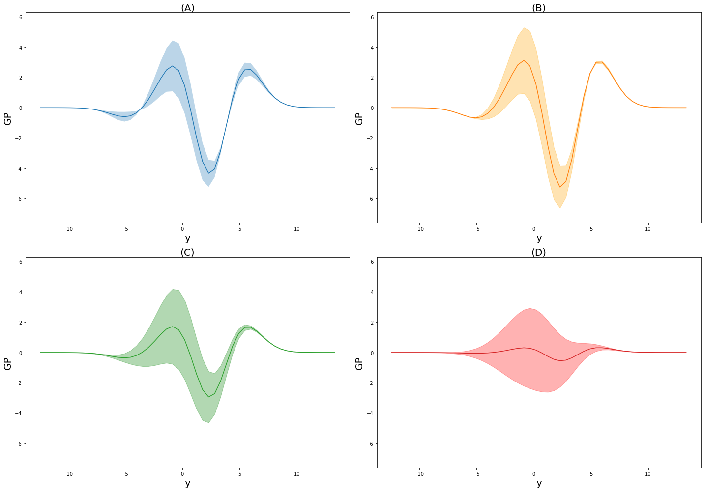
Figure 1: Illustration of the GP defining the posterior distribution of an example of a counterfactual mean embedding considered. The sample $\bf{x}^{\prime}$ is defined as $\bf{x}+$ shift, where (A) shift = 5, (B) shift = 7, (C) shift = 9, (D) shift = 11.

In contrast to CFME, BayesCFME provides with uncertainty estimates. The mean embedding itself encloses the aleatoric uncertainty of the counterfactual i.e. the counterfactual distribution itself. The uncertainty estimates of the BayesCFME model the epistemic uncertainty, as they are obtained due to lack of information. Figure 2 illustrates the comparison between the frequentist counterfactual mean embedding with kernel $K_{y}$ and the Bayesian counterfactual mean embedding with prior nuclear dominant kernel $R_{y}$. The introduction of the nuclear dominant kernel in the Bayesian approach results in the frequentist counterfactual mean embedding being different to the mean of the Bayesian counterfactual mean embedding.

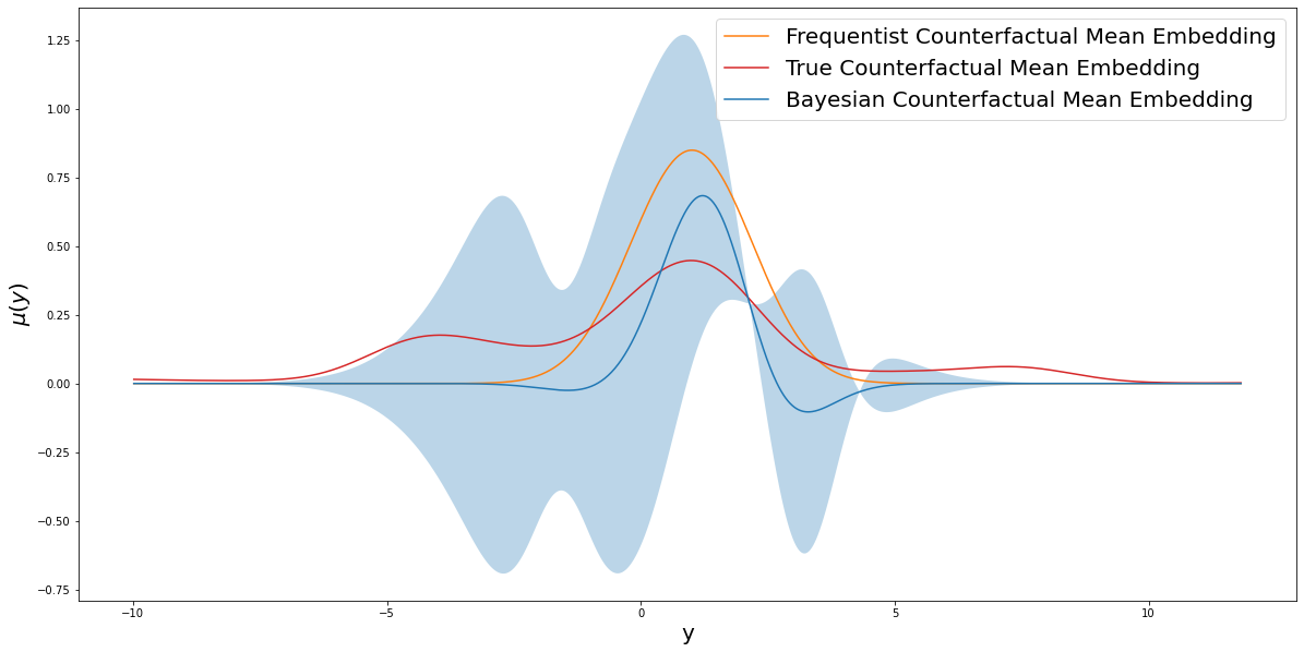
Figure 2: Illustration of the true counterfactual mean embedding, the frequentist counterfactual mean embedding considered in Muandet et al. (2017), and the Bayesian counterfactual mean embedding introduced in this work.

One may be interested in the BayesCFME for a variety reasons. Firstly, considering a Bayesian approach of the CFME for more than one group allows for a Bayesian kernel two-sample testing (Zhang et al. (2022)). Furthermore, the BayesCFME may be used for calculating the expectation of functions with respect to $\mathbb{P}_{Y\langle 0|1\rangle}$, given that they belong to the respective RKHS. The uncertainty estimates provided by BayesCFME allow for uncertainty on the predicted expectation. The idea is analogous to the one used in Bayesian Counterfactual Mean Embedding, which will be discussed in the next section (but with no need to estimate the function of interest).

Please note that BayesCFME may also be applied to the off-policy evaluation problem, with the only difference that the sample $\{x_{i}\}_{i=1}^{n}=\{u_{i},a_{i}\}_{i=1}^{n}$ from Proposition 2 is partially generated, given that we ought to simulate $a_{i}|u_{i}$ from the proposed policy.

5 A Bayesian approach for the off-policy evaluation problem

We now propose three estimators for the problem introduced in Subsection 3.2, based on the ideas presented in Chau et al. (2021a). Similarly to Chau et al. (2021a), we propose two-staged estimators that take into account uncertainties stemming from different data sources. However, the main difference is that the algorithms presented in Chau et al. (2021a) are designed to estimate the effect of an intervention, while we address a counterfactual problem.

Let’s suppose that we are given samples $D_{1}=\{(x_{i},r_{i})\}_{i=1}^{N}\sim\mathbb{P}_{X_{0},Y_{0}}$, $D_{2}=\{(\tilde{r_{j}},f(\tilde{r_{j}})+\xi_{j})\}_{j=1}^{M}$, $D_{3}=\{x^{\prime}_{l}\}_{l=1}^{L}\sim\mathbb{P}_{X_{1}}$, and the goal is to estimate $\mathbb{E}[f(R)]$, where $R\sim\mathbb{P}_{Y\langle 0|1\rangle}$. For simplicity of notation, we denote $y_{j}=f(\tilde{r_{j}})+\xi_{j}$. Alternatively, we can define the analogous off-policy problem where $D_{1}=\{(u_{i},a_{i},r_{i})\}_{i=1}^{N}\sim\mathbb{P}_{U,A,R}$, $D_{2}$ is defined in the same way, and $D_{3}=\{(u^{\prime}_{l},a^{\prime}_{l})\}_{l=1}^{L}\sim\mathbb{P}^{*}$, which is the target policy. In this case, part of $D_{3}$ is to be generated by the policy maker. However, we can refer to $(u,a)$ as $x$, given that variables $u$ and $a$ play the same role from a mathematical point of view.

Following a structure similar to Chau et al. (2021a), we propose two-staged estimators. On the one hand, we estimate $\mathbb{P}_{R}$ (distributional OPE) based on $D_{1}$ and $D_{3}$. On the other hand, we estimate $f(r):=\mathbb{E}_{p}[Y|r]$ given $D_{2}$. We consider three alternatives in this framework, which differ on whether a GP or a frequentist approach is used for the estimation of $\mathbb{P}_{R}$ and $f$:

• Counterfactual Mean Process (CFMP): The expectation $f(r)$ is trained as a GP and $\mu_{R\langle 0,1\rangle}$ is modeled by CFME.

• Bayesian Regressing Counterfactual Mean Embedding (BayesRCFME): The expectation $f(r)$ is modeled as a real-valued kernel ridge regression and and $\mu_{R\langle 0,1\rangle}$ is trained as a BayesCFME.

• Bayesian Counterfactual Mean Process (BayesCFMP): The expectation $f(r)$ is trained as a GP and and $\mu_{R\langle 0,1\rangle}$ is trained as a BayesCFME.

While the first two options fail to capture the uncertainty inherited by $D_{1}$ and $D_{2}$ respectively, BayesCFMP encompasses uncertainty derived from both data sets. Similarly to the algorithms presented Chau et al. (2021a), closed form solutions exist for the three approaches introduced thereof. While the algorithms exhibited in Chau et al. (2021a) have to account for an adjustment set, the proposed methods have to average the mean embeddings over $D_{3}$, hence using the counterfactual mean embedding. However, the proofs of the propositions are analogous. We state the closed forms in here for completeness, and we refer Chau et al. (2021a) for their derivations. We start by introducing the closed form solution of CFMP.

Proposition 3 (Counterfactual Mean Process (CFMP))

Let $k_{u},k_{a},k_{r}$ be the kernels associated to variables $u,a,k$ respectively and $D_{1}=\{(u_{i},a_{i},r_{i})\}_{i=1}^{N}=\{(x_{i},r_{i})\}_{i=1}^{N}$, $D_{2}=\{(\tilde{r}_{j},y_{j})\}_{j=1}^{M}$ two unmatched datasets . Furthermore, let $D_{3}=\{(u_{i}^{\prime},a_{i}^{\prime})\}_{i=1}^{L}=\{x^{\prime}\}_{i=1}^{L}$ be sampled from $\mathbb{P}^{*}$. We denote $\Phi(x)=\Phi(s,a)=\Phi_{\bf{s}}^{T}k_{s}(s,\cdot)\odot\Phi_{\bf{a}}^{T}k_{a}(a,\cdot)$. If $f$ is the posterior GP learnt form $D_{2}$, then $\eta=\int f(r)q^{*}(r)\sim\mathcal{N}(\mu_{1},\sigma^{2}_{1})$ where:

$$\mu_{1} =\langle\hat{\mu}_{R\langle 0,1\rangle},m_{f}\rangle=\frac{1}{L}1_{L}^{\top}K_{\bf{x^{\prime}}{\bf x}}(K+\lambda I)^{-1}K_{{\bf r}\tilde{{\bf r}}}(K_{\tilde{{\bf r}}\tilde{{\bf r}}}+\lambda_{f}I)^{-1}y,$$ (19)

$$\sigma^{2}_{1} =\mu_{Y\langle 0|1\rangle}^{\top}\mu_{Y\langle 0|1\rangle}-\mu_{Y\langle 0|1\rangle}^{\top}\Phi_{\tilde{{\bf r}}}(K_{\tilde{{\bf r}}\tilde{{\bf r}}}+\lambda I)^{-1}\Phi_{\tilde{{\bf r}}}^{\top}\mu_{Y\langle 0|1\rangle}$$ (20)

$$=\frac{1}{L^{2}}1_{L}^{\top}K_{\bf{x^{\prime}}{\bf x}}(K+\lambda I)^{-1}\tilde{K}_{{\bf r}{\bf r}}(K+\lambda I)^{-1}K_{{\bf x}\bf{x^{\prime}}}1_{L},$$ (21)

where $K_{\tilde{{\bf r}}{\bf r}}=\Phi_{\tilde{{\bf r}}}^{\top}\Phi_{{\bf r}}$, $m_{f}$ and $\tilde{K}_{{\bf r}{\bf r}}$ are the posterior mean function and covariance of $f$ evaluated at $r$. $\lambda>0$ is the regularization parameter and $\lambda_{f}$ is the noise term for the GP.

In CFMP, the GP $f$ is not required to be in any RKHS. In contrast, nuclear dominance is needed in the next two approaches. They exploit the fact that kernel mean embeddings may be used to compute the expectation of $f$ through the inner product, but $f$ ought to be in the respective RKHS (Lemma 1). The closed form of the BayesRCFME expressions follow.

Proposition 4 (Bayesian Regressing Counterfactual Mean Embedding (BayesRCFME))

Let $k_{u}$, $k_{a}$, $k_{r}$ be the kernels associated to variables $u,a,k$ respectively and $D_{1}=\{(u_{i},a_{i},r_{i})\}_{i=1}^{N}=\{(x_{i},r_{i})\}_{i=1}^{N}$, $D_{2}=\{(\tilde{r}_{j},y_{j})\}_{j=1}^{M}$ two unmatched datasets. Let $D_{3}=\{(u_{i}^{\prime},a_{i}^{\prime})\}_{i=1}^{L}=\{x^{\prime}\}_{i=1}^{L}$ be sampled from $\mathbb{P}^{*}$. We denote $\Phi(x)=\Phi(s,a)=\Phi_{\bf{s}}^{T}k_{s}(s,\cdot)\odot\Phi_{\bf{a}}^{T}k_{a}(a,\cdot)$. If $f$ is a KRR learnt form $D_{2}$ and $\mu_{Y\langle 0|1\rangle}$ modelled as a V-GP using $D_{1}$, then $\eta=\langle f,\mu_{Y\langle 0|1\rangle}\rangle\sim\mathcal{N}(\mu_{2},\sigma^{2}_{2})$, where

$$\mu_{2} =\frac{1}{L}1_{L}^{\top}K_{\bf{x^{\prime}}{\bf x}}(K_{{\bf x}{\bf x}}+\lambda I)^{-1}K_{{\bf r}{\bf r}}R_{{\bf r}{\bf r}}^{-1}R_{{\bf r}\bf\tilde{r}}A,$$ (22)

$$\sigma^{2}_{2} =B\frac{1}{L^{2}}1_{L}^{\top}K_{\bf{x^{\prime}}\bf{x^{\prime}}}1_{L}-C\frac{1}{L^{2}}1_{L}^{\top}K_{\bf{x^{\prime}}{\bf x}}(K_{{\bf x}{\bf x}}+\lambda I)^{-1}K_{{\bf x}\bf{x^{\prime}}}1_{L},$$ (23)

where $A=(K_{\bf\tilde{r}\bf\tilde{r}}+\lambda_{f}I)^{-1}y$, $B=A^{T}R_{\bf\tilde{r}\bf\tilde{r}}A$, and $C=A^{T}R_{\bf\tilde{r}{\bf r}}R_{{\bf r}{\bf r}}^{-1}R_{{\bf r}\bf\tilde{r}}A$.

Thirdly, we present the closed form solutions of BayesCFMP, which accounts for both sources of uncertainty.

Proposition 5 (Bayesian Counterfactual Mean Process (BayesCFMP))

Let $k_{u}$, $k_{a}$, $k_{r}$ be the kernels associated to variables $u,a,k$ respectively and $D_{1}=\{(u_{i},a_{i},r_{i})\}_{i=1}^{N}=\{(x_{i},r_{i})\}_{i=1}^{N}$, $D_{2}=\{(\tilde{r}_{j},y_{j})\}_{j=1}^{M}$ two unmatched datasets. Let $D_{3}=\{(u_{i}^{\prime},a_{i}^{\prime})\}_{i=1}^{L}=\{x^{\prime}\}_{i=1}^{L}$ be sampled from $\mathbb{P}^{*}$. We denote $\Phi(x)=\Phi(s,a)=\Phi_{\bf{s}}^{T}k_{s}(s,\cdot)\odot\Phi_{\bf{a}}^{T}k_{a}(a,\cdot)$, and $\hat{{\bf r}}=({\bf r},\tilde{{\bf r}})$. If $f$ and $\mu_{Y\langle 0|1\rangle}$ are modeled as GP, then $\eta=\langle f,\mu_{Y\langle 0|1\rangle}\rangle$ has the following mean $\mu_{3}$ and variance $\sigma^{2}_{3}$:

$$\mu_{3} =EK_{{\bf r}\bf\hat{r}}K_{\bf\hat{r}\bf\hat{r}}^{-1}R_{\bf\hat{r}\bf\tilde{r}}(R_{\bf\tilde{r}\bf\tilde{r}}+\lambda_{f}I)^{-1}y,$$ (24)

$$\sigma^{2}_{3} =E\Theta_{1}^{\top}\bar{R}_{\bf\hat{r}\bf\hat{r}}\Theta_{1}E^{\top}+\Theta_{2}^{(a)}F-\Theta_{2}^{(b)}G+\Theta_{3}^{(a)}F-\Theta_{3}^{(b)}G,$$ (25)

where $E=\frac{1}{L}1_{L}^{\top}K_{\bf{x^{\prime}}{\bf x}}(K_{{\bf x}{\bf x}}+\lambda I)^{-1}$, $F=\frac{1}{L^{2}}1_{L}^{\top}K_{\bf{x^{\prime}}\bf{x^{\prime}}}1_{L}$, $G=\frac{1}{L^{2}}1_{L}^{\top}K_{\bf{x^{\prime}}{\bf x}}(K_{{\bf x}{\bf x}}+\lambda I)^{-1}K_{{\bf x}\bf{x^{\prime}}}1_{L}$, $\Theta_{1}=K_{\bf\hat{r}\bf\hat{r}}^{-1}R_{\bf\hat{r}{\bf r}}R_{{\bf r}{\bf r}}^{-1}K_{{\bf r}{\bf r}}$, $\Theta_{2}^{(a)}=\Theta_{4}^{\top}R_{\bf\hat{r}\bf\hat{r}}\Theta_{4}$, $\Theta_{2}^{(b)}=\Theta_{4}^{\top}R_{\bf\hat{r}{\bf r}}R_{{\bf r}{\bf r}}^{-1}R_{{\bf r}\bf\hat{r}}\Theta_{4}$, $\Theta_{3}^{(a)}=tr(K_{\bf\hat{r}\bf\hat{r}}^{-1}R_{\bf\hat{r}\bf\hat{r}}K_{\bf\hat{r}\bf\hat{r}}^{-1}\bar{R}_{\bf\hat{r}\bf\hat{r}})$, $\Theta_{3}^{(b)}=tr(R_{\bf\hat{r}{\bf r}}R_{{\bf r}{\bf r}}^{-1}R_{{\bf r}\bf\hat{r}}K_{\bf\hat{r}\bf\hat{r}}^{-1}\bar{R}_{\bf\hat{r}\bf\hat{r}}K_{\bf\hat{r}\bf\hat{r}}^{-1})$, $\Theta_{4}=K_{\bf\hat{r}\bf\hat{r}}^{-1}R_{\bf\hat{r}\bf\tilde{r}}(K_{\bf\tilde{r}\bf\tilde{r}}+\lambda_{f})^{-1}y$, . $\bar{R}_{\bf\hat{r}\bf\hat{r}}$ is the posterior covariance of f evaluated at $\hat{{\bf r}}$.

6 Experiments

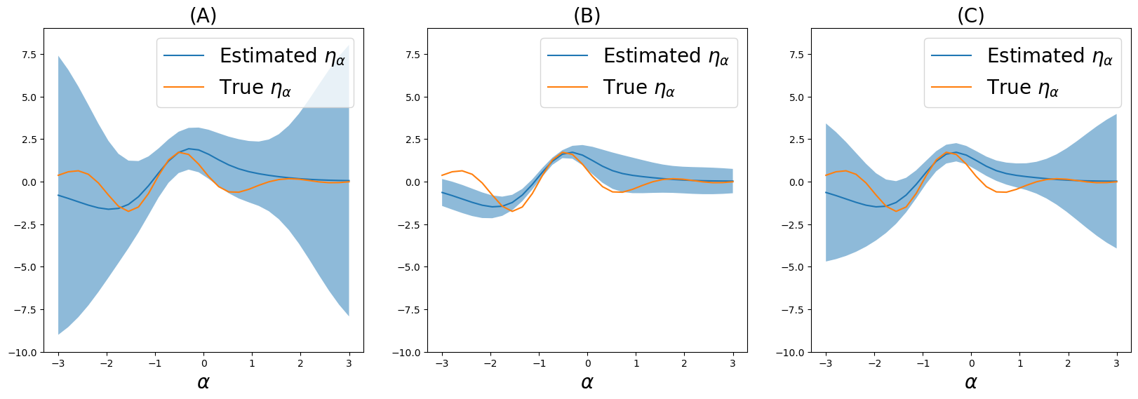
Figure 3: Illustration of the experiment conducted on setting A. The mean and uncertainty estimates (95% CI) of $\eta_{\alpha}$ are displayed for (A) BayesCFMP, (B) CFMP, (C) BayesCFME.

In order to illustrate the performance of the proposed algorithms, two simulated experimental settings are considered on different off-policy evaluation problems (please note that the counterfactual estimation problem presented in Section 5 could be understood as a specific example of the OPE problem as stated in Subsection 3.1). For each of the examples, we work with two generated data sets $D_{1}=\{(u_{i},a_{i},r_{i})\}_{i=1}^{N}$ (collected from the logging policy) and $D_{2}=\{(\tilde{r}_{j},y_{j})\}_{j=1}^{M}$. We then propose a set of new policies $\mathbb{P}_{A|U}^{\alpha}(a|u)$, where $\alpha\in\Lambda\subset\mathbb{R}$. The goal is to estimate $\eta_{\alpha}$ (ultimate effect of policy $\mathbb{P}^{\alpha}$) and to provide with uncertainty estimates accounting for the reliability of the measurement.

The results of the simulations conducted on two different settings, namely A and B, are exhibited in Figure 3 and Figure 4 respectively. We refer the reader to Appendix A for the details of the experimental settings considered, as well as additional experimental results for the two settings with different parameters. The mean and a 95% CI (obtained from the variance estimate determined by the algorithms) are provided for every $\alpha$ for BayesCFMP, BayesRCFME and CFMP. The true expected ultimate reward is also displayed, which is unknown in real life applications. We have chosen two representative examples to illustrate how BayesCFME rectifies the deficiencies shown by CFMP and BayesRCFME by quantifying uncertainty corresponding to both data sets. All kernels considered were taken as RBF kernels.

In setting A (Figure 3), the true $\eta_{\alpha}$ lies outside the 95% confident region for BayesRCFME for values of $\alpha$ close to 0. CFMP estimates suffer as well for low values of $\alpha$. Nonetheless, BayesCFMP uncertainty estimates seem to be best calibrated. In setting B (Figure 4), the true $\eta_{\alpha}$ lies outside 95% CI provided by BayesCFME and CFMP in most of the $\Lambda=[-8,8]$ considered. The uncertainty quantification seems to be well calibrated when considering the two sources of uncertainty through BayesCFMP.

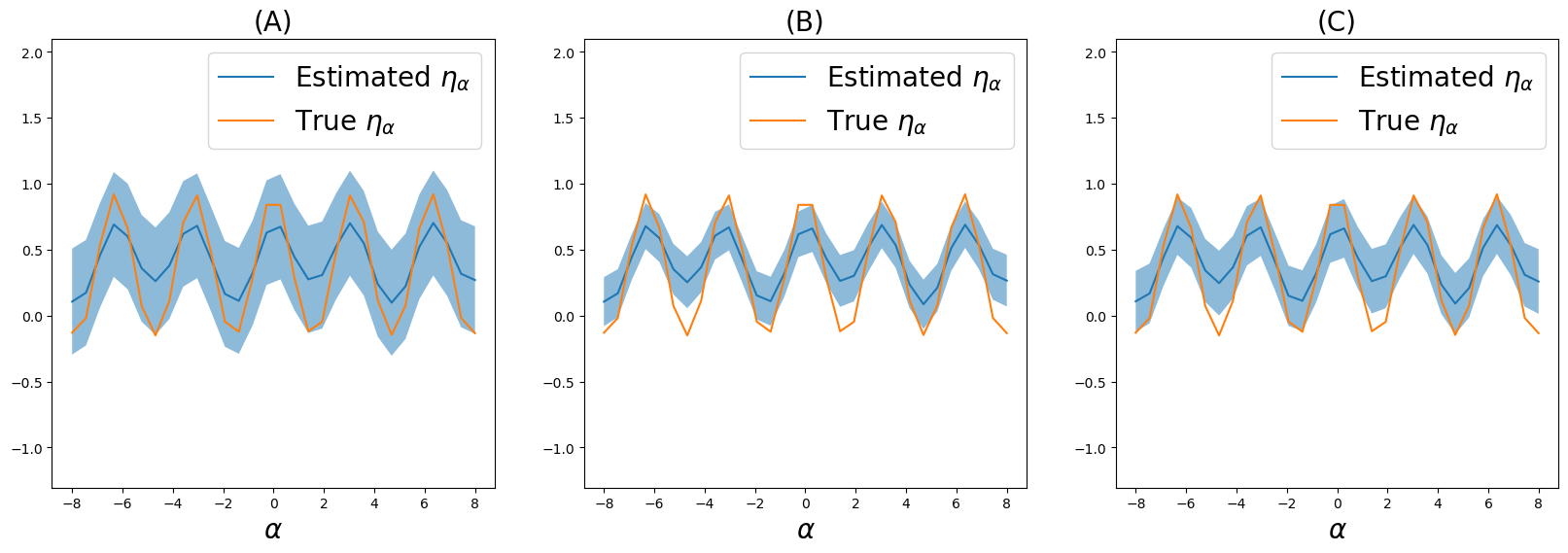
Figure 4: Illustration of the experiment conducted on setting B. The mean and uncertainty estimates (95% CI) of $\eta_{\alpha}$ are displayed for (A) BayesCFMP, (B) CFMP, (C)BayesCFME.

7 Conclusion and future work

We have presented a Bayesian approach for the counterfactual distribution estimation problem based on Bayesian conditional mean embeddings. Such approach may be combined with the estimation of an unknown function in order to yield uncertainty estimates for the expectation of such function with respect to the counterfactual distribution. Building on the ideas presented in Chau et al. (2021a), we have proposed three methods for such task which differ in the sources of uncertainty considered. Furthermore, these techniques may also be applied to the off-policy evaluation framework, which can be seen as a generalization of the aforementioned problem. We have empirically compared the three proposed methods in two experimental settings, showing the value of considering the uncertainty stemming from the two different sources of data.

A line of research that could naturally follow this work is the exploration of a Bayesian kernel approach for distributional treatment effects, where the distribution of the treated and untreated has to be accounted for. This would open the door for two sample Bayesian tests for distributional treatment effects. A ‘functional’ treatment effect, where the expectation would be taken over a (potentially estimated) function of the treatment effect, could also be addressed using such methodology. Moreover, studying closed-form solutions or approximations for nuclear dominant kernels other than Gaussian would open the door for doing model selection in the framework proposed, with the consequent computational and theoretical advantages.

Appendix A Experimenal settings

In order to explore the performance of the proposed algorithms, two experimental settings are considered. For each of the examples, we work with two generated data sets $D_{1}=\{(u_{i},a_{i},r_{i})\}_{i=1}^{N}$ and $D_{2}=\{(\tilde{r}_{j},y_{j})\}_{j=1}^{M}$. We then propose a set of new policies $\mathbb{P}_{A|U}^{\alpha}(a|u)$, where $\alpha\in\Lambda\subset\mathbb{R}$. We assume that $\mathbb{P}_{U}^{\alpha}(u)$ is invariant with respect to the historic data, thus we keep the given data $\bf{u}$ for the new policies (usual setting). The goal is to estimate $\eta_{\alpha}$, and to provide with uncertainty estimates accounting for the reliability of the measurement. All kernels considered were taken as RBF kernels. The two settings are defined such that:

1. Setting A:

   • $u_{i}\sim\mathcal{N}(5,2)$.

   • $\tilde{r_{j}}\sim Uniform(-2,2)$.

   • $a_{i}|u_{i}\sim 4\mathcal{N}(0,1)$.

   • $r_{i}|u_{i},a_{i}\sim(u_{i}+a_{i})+0.05\mathcal{N}(0,1)$

   • $y_{j}|\tilde{r}_{j}\sim 2\sin{(\tilde{r}_{j}/2)}+0.05\mathcal{N}(0,1)$.

   • $\mathbb{P}_{A|U}^{\alpha}(a|u)\sim\alpha u+0.05\mathcal{N}(0,1)$.

2. Setting B:

   • $u_{i}\sim\mathcal{N}(5,2)$.

   • $\tilde{r_{j}}\sim Uniform(-2,2)$.

   • $a_{i}|u_{i}\sim 3\mathcal{N}(0,1)$.

   • $r_{i}|u_{i},a_{i}\sim\cos{u_{i}}+\sin{a_{i}}+0.5\mathcal{N}(0,1)$

   • $y_{j}|\tilde{r}_{j}\sim 1.5\sin{\tilde{r}_{j}}+0.2\mathcal{N}(0,1)$.

   • $\mathbb{P}_{A|U}^{\alpha}(a|u)\sim 2\sin{\alpha}+0.5\mathcal{N}(0,1)$.

For both settings, we consider the parameters:

• $N\in\{100,200\}$.

• $M\in\{100,200\}$.

We exhibit the results of the experiments corresponding to Setting A and Setting B in Figure 5 and Figure 6 respectively.

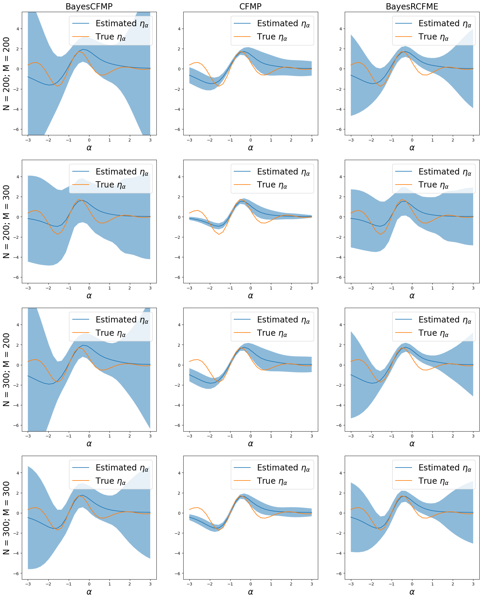
Figure 5: Illustration of the experiment conducted on setting A. The mean and uncertainty estimates (95% CI) of $\eta_{\alpha}$ are displayed for BayesCFMP, CFMP, and BayesCFME.

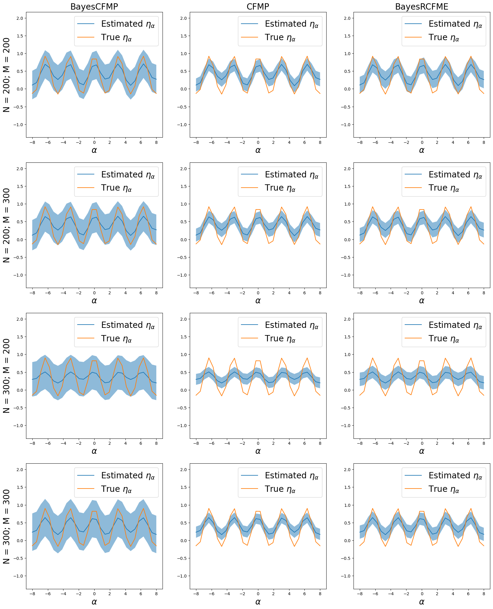
Figure 6: Illustration of the experiment conducted on setting A. The mean and uncertainty estimates (95% CI) of $\eta_{\alpha}$ are displayed for BayesCFMP, CFMP, and BayesCFME.

References

- Soize [2017] Christian Soize. Uncertainty quantification. Springer, 2017.
- Psaros et al. [2022] Apostolos F Psaros, Xuhui Meng, Zongren Zou, Ling Guo, and George Em Karniadakis. Uncertainty quantification in scientific machine learning: Methods, metrics, and comparisons. arXiv preprint arXiv:2201.07766, 2022.
- Sullivan [2015] Timothy John Sullivan. Introduction to uncertainty quantification, volume 63. Springer, 2015.
- Monteiro et al. [2020] Miguel Monteiro, Loïc Le Folgoc, Daniel Coelho de Castro, Nick Pawlowski, Bernardo Marques, Konstantinos Kamnitsas, Mark van der Wilk, and Ben Glocker. Stochastic segmentation networks: Modelling spatially correlated aleatoric uncertainty. Advances in Neural Information Processing Systems, 33:12756–12767, 2020.
- Wang et al. [2019] Guotai Wang, Wenqi Li, Michael Aertsen, Jan Deprest, Sébastien Ourselin, and Tom Vercauteren. Aleatoric uncertainty estimation with test-time augmentation for medical image segmentation with convolutional neural networks. Neurocomputing, 338:34–45, 2019.
- Larrañaga and Lozano [2001] Pedro Larrañaga and Jose A Lozano. Estimation of distribution algorithms: A new tool for evolutionary computation, volume 2. Springer Science & Business Media, 2001.
- Begoli et al. [2019] Edmon Begoli, Tanmoy Bhattacharya, and Dimitri Kusnezov. The need for uncertainty quantification in machine-assisted medical decision making. Nature Machine Intelligence, 1(1):20–23, 2019.
- Vishwakarma et al. [2021] Gaurav Vishwakarma, Aditya Sonpal, and Johannes Hachmann. Metrics for benchmarking and uncertainty quantification: Quality, applicability, and best practices for machine learning in chemistry. Trends in Chemistry, 3(2):146–156, 2021.
- Sugiyama et al. [2008] Masashi Sugiyama, Taiji Suzuki, Shinichi Nakajima, Hisashi Kashima, Paul von Bünau, and Motoaki Kawanabe. Direct importance estimation for covariate shift adaptation. Annals of the Institute of Statistical Mathematics, 60(4):699–746, 2008.
- Zhou and Levine [2021] Aurick Zhou and Sergey Levine. Bayesian adaptation for covariate shift. Advances in Neural Information Processing Systems, 34:914–927, 2021.
- Pearl [2003] Judea Pearl. Causality: Models, reasoning, and inference. Econometric Theory, 19:675–685, 2003.
- Chernozhukov et al. [2013] Victor Chernozhukov, Iván Fernández-Val, and Blaise Melly. Inference on counterfactual distributions. Econometrica, 81(6):2205–2268, 2013.
- Westreich and Cole [2010] Daniel Westreich and Stephen R Cole. Invited commentary: positivity in practice. American journal of epidemiology, 171(6):674–677, 2010.
- Petersen et al. [2012] Maya L Petersen, Kristin E Porter, Susan Gruber, Yue Wang, and Mark J Van Der Laan. Diagnosing and responding to violations in the positivity assumption. Statistical methods in medical research, 21(1):31–54, 2012.
- Léger et al. [2022] Maxime Léger, Arthur Chatton, Florent Le Borgne, Romain Pirracchio, Sigismond Lasocki, and Yohann Foucher. Causal inference in case of near-violation of positivity: comparison of methods. Biometrical Journal, 2022.
- Greenland and Robins [1986] Sander Greenland and James M Robins. Identifiability, exchangeability, and epidemiological confounding. International journal of epidemiology, 15(3):413–419, 1986.
- Maei et al. [2010] Hamid Reza Maei, Csaba Szepesvári, Shalabh Bhatnagar, and Richard S Sutton. Toward off-policy learning control with function approximation. In ICML, 2010.
- Smola et al. [2007] Alex Smola, Arthur Gretton, Le Song, and Bernhard Schölkopf. A hilbert space embedding for distributions. In International Conference on Algorithmic Learning Theory, pages 13–31. Springer, 2007.
- Song et al. [2009] Le Song, Jonathan Huang, Alex Smola, and Kenji Fukumizu. Hilbert space embeddings of conditional distributions with applications to dynamical systems. In Proceedings of the 26th Annual International Conference on Machine Learning, pages 961–968, 2009.
- Flaxman et al. [2016] Seth Flaxman, Dino Sejdinovic, John P. Cunningham, and Sarah Filippi. Bayesian learning of kernel embeddings, 2016. URL https://arxiv.org/abs/1603.02160.
- Chau et al. [2021a] Siu Lun Chau, Jean-François Ton, Javier González, Yee Whye Teh, and Dino Sejdinovic. Bayesimp: Uncertainty quantification for causal data fusion, 2021a.
- Lukić and Beder [2001] Milan Lukić and Jay H. Beder. Stochastic processes with sample paths in reproducing kernel hilbert spaces. Transactions of the American Mathematical Society, 353:3945–3969, 2001.
- Melly [2006] Blaise Melly. Estimation of counterfactual distributions using quantile regression. University of St.Gallen, 68, 01 2006.
- Kennedy et al. [2021] Edward H Kennedy, Sivaraman Balakrishnan, and Larry Wasserman. Semiparametric counterfactual density estimation. arXiv preprint arXiv:2102.12034, 2021.
- Johansson et al. [2016] Fredrik Johansson, Uri Shalit, and David Sontag. Learning representations for counterfactual inference. In International conference on machine learning, pages 3020–3029. PMLR, 2016.
- Thomas and Brunskill [2016] Philip Thomas and Emma Brunskill. Data-efficient off-policy policy evaluation for reinforcement learning. In International Conference on Machine Learning, pages 2139–2148. PMLR, 2016.
- Swaminathan et al. [2017] Adith Swaminathan, Akshay Krishnamurthy, Alekh Agarwal, Miro Dudik, John Langford, Damien Jose, and Imed Zitouni. Off-policy evaluation for slate recommendation. Advances in Neural Information Processing Systems, 30, 2017.
- Huang et al. [2021] Audrey Huang, Liu Leqi, Zachary C. Lipton, and Kamyar Azizzadenesheli. Off-policy risk assessment in contextual bandits. CoRR, abs/2104.08977, 2021. URL https://arxiv.org/abs/2104.08977.
- Chandak et al. [2021] Yash Chandak, Scott Niekum, Bruno Castro da Silva, Erik G. Learned-Miller, Emma Brunskill, and Philip S. Thomas. Universal off-policy evaluation. CoRR, abs/2104.12820, 2021. URL https://arxiv.org/abs/2104.12820.
- Taufiq et al. [2022] Muhammad Faaiz Taufiq, Jean-Francois Ton, Rob Cornish, Yee Whye Teh, and Arnaud Doucet. Conformal off-policy prediction in contextual bandits, 2022. URL https://arxiv.org/abs/2206.04405.
- Muandet et al. [2021] Krikamol Muandet, Motonobu Kanagawa, Sorawit Saengkyongam, and Sanparith Marukatat. Counterfactual mean embeddings, 2021.
- Muandet et al. [2017] Krikamol Muandet, Kenji Fukumizu, Bharath Sriperumbudur, and Bernhard Schölkopf. Kernel mean embedding of distributions: A review and beyond. Foundations and Trends® in Machine Learning, 10(1-2):1–141, 2017. doi:10.1561/2200000060. URL https://doi.org/10.1561%2F2200000060.
- Gretton et al. [2012] Arthur Gretton, Karsten M Borgwardt, Malte J Rasch, Bernhard Schölkopf, and Alexander Smola. A kernel two-sample test. The Journal of Machine Learning Research, 13(1):723–773, 2012.
- Grunewalder et al. [2012] Steffen Grunewalder, Guy Lever, Luca Baldassarre, Massi Pontil, and Arthur Gretton. Modelling transition dynamics in mdps with rkhs embeddings. arXiv preprint arXiv:1206.4655, 2012.
- Singh et al. [2019] Rahul Singh, Maneesh Sahani, and Arthur Gretton. Kernel instrumental variable regression. Advances in Neural Information Processing Systems, 32, 2019.
- Singh et al. [2021] Rahul Singh, Liyuan Xu, and Arthur Gretton. Kernel methods for multistage causal inference: Mediation analysis and dynamic treatment effects. arXiv preprint arXiv:2111.03950, 2021.
- Chau et al. [2021b] Siu Lun Chau, Shahine Bouabid, and Dino Sejdinovic. Deconditional downscaling with gaussian processes. Advances in Neural Information Processing Systems, 34:17813–17825, 2021b.
- Martinez-Taboada and Sejdinovic [2022] Diego Martinez-Taboada and Dino Sejdinovic. Sequential decision making on unmatched data using bayesian kernel embeddings, 2022. URL https://arxiv.org/abs/2210.13692.
- Wang et al. [2017] Yu-Xiang Wang, Alekh Agarwal, and Miroslav Dudık. Optimal and adaptive off-policy evaluation in contextual bandits. In International Conference on Machine Learning, pages 3589–3597. PMLR, 2017.
- Geist et al. [2014] Matthieu Geist, Bruno Scherrer, et al. Off-policy learning with eligibility traces: a survey. J. Mach. Learn. Res., 15(1):289–333, 2014.
- Sugiyama and Storkey [2006] Masashi Sugiyama and Amos J Storkey. Mixture regression for covariate shift. Advances in neural information processing systems, 19, 2006.
- Kato et al. [2020] Masahiro Kato, Masatoshi Uehara, and Shota Yasui. Off-policy evaluation and learning for external validity under a covariate shift, 2020. URL https://arxiv.org/abs/2002.11642.
- Rockafellar et al. [2000] R Tyrrell Rockafellar, Stanislav Uryasev, et al. Optimization of conditional value-at-risk. Journal of risk, 2:21–42, 2000.
- Zhu and Fukushima [2009] Shushang Zhu and Masao Fukushima. Worst-case conditional value-at-risk with application to robust portfolio management. Operations Research, 57:1155–1168, 10 2009. doi:10.1287/opre.1080.0684.
- Meng et al. [2020] Tong Meng, Xuyang Jing, Zheng Yan, and Witold Pedrycz. A survey on machine learning for data fusion. Information Fusion, 57:115–129, 2020.
- Fukumizu et al. [2007] Kenji Fukumizu, Arthur Gretton, Xiaohai Sun, and Bernhard Schölkopf. Kernel measures of conditional dependence. Advances in neural information processing systems, 20, 2007.
- Grünewälder et al. [2012] Steffen Grünewälder, Guy Lever, Luca Baldassarre, Sam Patterson, Arthur Gretton, and Massimilano Pontil. Conditional mean embeddings as regressors - supplementary. arXiv e-prints, art. arXiv:1205.4656, May 2012.
- Zhang et al. [2022] Qinyi Zhang, Veit Wild, Sarah Filippi, Seth Flaxman, and Dino Sejdinovic. Bayesian kernel two-sample testing. Journal of Computational and Graphical Statistics, 0(0):1–13, 2022. doi:10.1080/10618600.2022.2067547. URL https://doi.org/10.1080/10618600.2022.2067547.