Implicit Neural Representation as a Differentiable Surrogate for Photon Propagation in a Monolithic Neutrino Detector

Abstract

Optical photons are used as signal in a wide variety of particle detectors. Modern neutrino experiments employ hundreds to tens of thousands of photon detectors to observe signal from millions to billions of scintillation photons produced from energy deposition of charged particles. These neutrino detectors are typically large, containing $\mathcal{O}(10^{2}~{}-~{}10^{5})$ tons of target volume, and may consist of many materials with different optical properties. As a result, modeling individual photon propagation requires prohibitive computational resources. As an alternative to tracking individual photons, the experimental community has traditionally used a look-up table, which contains a mean probability of observing a photon per photon detector at each grid location in a uniformly voxelized detector volume. However, since the size of a table increases with detector volume for a fixed resolution, this method scales poorly for future larger detectors. Alternative approaches such as fitting a polynomial to the model could address the memory issue, but results in poorer performance. Furthermore, both look-up table and fitting approaches are prone to discrepancies between the detector simulation and the real-world detector response. We propose a new approach using SIREN, a implicit neural representation with periodic activation functions. In our approach, SIREN is used to model the look-up table as a “3D scene” and reproduces the acceptance map with high accuracy. The number of parameters in our SIREN model is orders of magnitude smaller than the number of voxels in the look-up table. As it models an underlying functional shape, SIREN is scalable to a larger detector. Furthermore, SIREN can successfully learn the spatial gradients of the photon library, providing additional information for downstream applications. Finally, as SIREN is a neural network representation, it is differentiable with respect to its parameters, and therefore tunable via gradient descent. We demonstrate the potential of optimizing SIREN directly on real data, which mitigates the concern of data vs. simulation discrepancies. We further present an application for data reconstruction where SIREN is used to form a likelihood function for photon statistics.

I Introduction

Liquid Argon Time Projection Chambers (LArTPC) are the detector technology of choice across the Department of Energy’s flagship accelerator-based neutrino experiments, including the Short Baseline Neutrino (SBN) program and the Deep Underground Neutrino Experiment (DUNE) Acciarri et al. ; Abud et al. . LArTPCs provide two detection modalities: charge and light. Neutrino interactions with Ar nuclei produce secondary particles; the charged particles ionize Ar atoms along their trajectories to produce electrons and scintillation photons. The electrons drift in an applied electric field and are recorded by a grid of detection wires Acciarri et al. (2017) or pixels Dwyer et al. (2018). The 3D position is reconstructed from one- or two-dimensional spatial measurements combined with the measured time. Scintillation photons travel isotropically and are measured by optical detectors. The electron signal is spatially precise but temporally coarse ($\order{$\mathrm{ms}$}$) while the photon signal is spatially coarse and temporally precise ($\order{$\mathrm{ns}$}$).

An important challenge in creating a full LArTPC simulation is the modeling of optical visibility, i.e. the probability of observing a photon produced at a given location in the detector volume. Optical visibility is estimated by generating a large number ($\order{10^{4}-10^{6}}$) of photons at a single location, propagating the generated photons through the detector volume, and recording the number of photons detected from the optical detectors. The current procedure is to create a lookup table called the photon library, where each step in estimating the optical visibility is repeated over the entire detector at equally spaced points of $\order{$\mathrm{cm}$}$ in each direction.

The generation of the photon library is slow and only redone if there is a change in the underlying detector properties. From a recent study of the ICARUS detector Rubbia et al. (2011), currently the world’s largest LArTPC in operation, it took about a week to generate a photon library of about 2 million sampling points with a $5\times 5\times 5~{}$\mathrm{cm}$^{3}$ voxel size. While the generated ICARUS photon library may stay fixed for downstream usage, it is already limited by the spatial resolution in physics modeling due to its memory footprint. It is therefore not feasible to apply the same strategy for larger detectors such as DUNE-FD Abi et al. (2020) ($\sim$100$\times$ ICARUS). Analytical approximations that require less memory have been proposed as alternatives to the photon library, but it is often challenging to explicitly express the underlying distribution using common functions. Furthermore, neither the photon library nor the analytical approximation are amenable to in situ calibration with detector data due to the slow regeneration time of the photon library. Therefore, even if these models could be made computationally efficient, they would still introduce biases from differences between simulation and data.

This paper will address these challenges by constructing a differentiable optical visibility from a neural implicit model. It is designed to learn the average photon yield at an optical detector from a given a continuous 3D position inside the detector Such a model is easily and quickly tunable via gradient descent, providing an efficient method of in situ calibration. As it is a continuous function, it drastically reduces the number of parameters needed for physics modeling relative to a voxel representation, and correspondingly has a much smaller memory footprint, allowing scalable modeling of optical information in large detectors.

II SIREN for Photon Propagation

Implicit neural representations are a novel way to parameterize signals as continuous functions via neural networks, which are trained to map the domain of the signal (e.g. spatial coordinates) to the target outputs (e.g. the signal at those coordinates). Recent advancements in neural scene representation have demonstrated that neural implicit models can represent 2D and 3D images containing high frequency features with the level of precision required by high energy physics Mildenhall et al. ; Martel et al. ; Sitzmann et al. .

Sinusoidal representation networks (SIRENs) Sitzmann et al. are implicit neural representations that use a simple multilayer perception (MLP) network architecture along with periodic sine function activations, i.e.,

$$\mathbf{\Phi}(\mathbf{x}) = \mathbf{W}_{n}(\phi_{n-1}\circ\phi_{n-2}\circ\dots\circ\phi_{0})(\mathbf{x})+\mathbf{b}_{n},$$

$$\phi_{i}(\mathbf{x}_{i}) = \sin(\mathbf{W}_{i}\mathbf{x}_{i}+\mathbf{b}_{i}),$$ (1)

where the function $\phi_{i}:\mathbb{R}^{M_{i}}\mapsto\mathbb{R}^{N_{i}}$ ($N_{i},M_{i}$ are positive integers) of the $i$-th layer of the network consists of an affine transform on the input $\mathbf{x}_{i}\in\mathbb{R}^{M_{i}}$ given by the weight matrix $\mathbf{W}_{i}\in\mathbb{R}^{N_{i}\times M_{i}}$ and the biases $\mathbf{b_{i}}\in\mathbb{R}^{N_{i}}$, followed by the sine activation applied on each component of the resulting vector. The input signal is parameterized as a continous function $\mathbf{\Phi}$ using the above architecture.

For application of photon propagation, an optical visibility map $\mathbf{\Psi}:\mathbb{R}^{3}\mapsto\mathbb{R}^{N_{d}}$ is modeled using SIREN. The function $\mathbf{\Psi}$ maps a coordinate $\mathbf{x}\in\mathbb{R}^{3}$ within the detection volume to the visibility of $N_{d}$ optical detector for the simulated ICARUS detector). There are three hyper-parameters for the SIREN model: number of hidden layers ($n_{L}$) with sinusoidal activation, number of hidden features ($n_{F}$) and a frequency factor $\omega$. In the models used for this work, all hidden layers have the same number of hidden features: $M_{i}=N_{i}=n_{F}$.

The frequency factor $\omega$ is introduced by factoring the weight matrix $\mathbf{W}\to\omega\mathbf{W}$ in order to increase the spatial frequency of the layers. This allows for a better match to the frequency spectrum of the signal and accelerates the training of SIREN in all hidden layers Sitzmann et al. , as discussed in Section IV.3.

As the parameterization $\mathbf{\Psi}$ is defined on the continuous domain of $\mathbf{x}$, it is not limited by a voxel grid resolution, allowing for the modeling of finer details than the standard lookup table photon library. It is also more memory efficient than such a discrete lookup table. The gradients and higher order derivatives with respect to the input coordinates can be computed in closed form instead of using the finite difference method. With the well-behaved derivatives, SIREN offers additional applications such as solving inverse problems. Further, as a neural network, SIREN is able to be optimized via gradient descent.

III Optimization

III.1 Voxel-wise Loss

Let $\mathcal{D}=\{\mathbf{x}_{i}\}\subset\mathbb{R}^{3}$ be a set of voxel coordinates and $v_{ij}$ be the visibility of position $\mathbf{x}_{i}$ at the $j$-th photon detector. The values of $v_{ij}$ are obtained from the optical detector simulation. The objective is to find a parameterization of the optical visibility $\mathbf{\Psi}(\mathbf{x})$ that minimizes the absolute bias ($b_{\mathrm{abs}})$ and relative bias ($b_{\mathrm{rel}}$), defined as

$$b_{\mathrm{abs}} = \left<|\mathbf{\Psi}_{j}(\mathbf{x}_{i})-v_{ij}|\right>,$$ (2)

$$b_{\mathrm{rel}} = \left<2\left|\frac{\mathbf{\Psi}_{j}(\mathbf{x}_{i})-v_{ij}}{\mathbf{\Psi}_{j}(\mathbf{x}_{i})+v_{ij}}\right|\right>,$$ (3)

where $\left<\cdot\right>$ denotes the arithmetic mean. The calculation of $b_{\mathrm{abs}}$ includes all data points and photomultiplier tubes (PMTs) in the sample, while $b_{\mathrm{rel}}$ has a threshold of $v_{ij}>4.5\times 10^{-5}$. Because of the uneven distribution of $v_{ij}$ in the photon library (Fig. 1), $b_{\mathrm{abs}}$ is statistically weighted toward the low-to-zero visibility region. In contrast, $b_{\mathrm{rel}}$ gives a better measure of the accuracy of reproducing the bright detector regions with SIREN.

To account for the high dynamic range of the visibility, which typically spans over several order of magnitude (Fig. 1), $v_{ij}$ is transformed into a logarithm scale $\tilde{v}_{ij}=\log_{10}(v_{ij}+\epsilon)$. A small constant $\epsilon=10^{-5}$ is added to avoid values of infinity at $v_{ij}=0$. For training of the SIREN, the input coordinates, $\mathbf{x}_{i}$, are normalized to lie within $[-1,1]$, and the logarithm of visibility is normalized to $[0,1]$.

The training of SIREN minimizes the squared error:

$$\mathcal{L}_{2}=\sum_{\mathbf{x}_{i}\in\mathcal{D}}\sum_{j=1}^{N_{d}}w_{ij}[\tilde{\Psi}_{j}(\mathbf{x}_{i})-\tilde{v}_{ij}]^{2},$$ (4)

where $w_{ij}$ is an optional precompuated weight, and $\mathbf{\tilde{\Psi}}$ is a parameterizaion of the visibility after logarithmic transformation as discussed above. The training sample $\mathcal{D}$ may be obtained from a photon library lookup table.

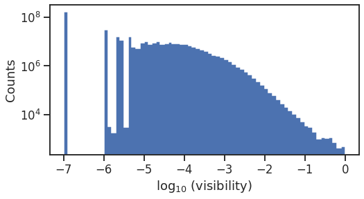
Figure 1: Distribution of the visibility of the ICARUS photon library. Data points with zero visibility are grouped into the first bin.

III.2 Track-wise Loss

The minimization of the voxel-wise loss $\mathcal{L}_{2}$ allows for a direct representation of the photon library via sampling of the visibility at different coordinates. However, the visibility of an individual voxel is not available in real data because there is no point-like calibration source in the LArTPC detector. Therefore, an alternative approach is required for working with data, where the only information is the readout of optical detectors from particle tracks

The basic principle of the track-wise loss is to associate the flashes from the optical detector to the charge readout of tracks in the LArTPC. The number of scintillation photons corresponding to an energy deposition in LAr is typically $\mathcal{O}(10^{4}-10^{5})$ photons/MeV depending on the magnitude of the drift field Cennini et al. (1995). The expected number of photoelectrons (PEs) $\lambda_{j}$ detected by the $j$-th PMT is given by

$$\lambda_{j}=\sum_{t\in\mathcal{T}}Y_{j}\times\Delta E_{t}\times\mathbf{\Psi}_{j}(\mathbf{x}_{t}),$$ (5)

where $\mathcal{T}$ is the collection of charge voxels occupied by an image of track(s), $Y_{j}$ is the PMT light yield, $\Delta E_{t}$ is the amount of the energy deposited in LAr at voxel $t$, and $\Psi_{j}(\mathbf{x}_{t})$ is the optical visibility at the voxel coordinates $\mathbf{x}_{t}$. The PMT light yield ($Y_{j}$) is a drift field dependent factor, which consists of the scintillation light yield, the PMT collection efficiency and the PMT gain for the conversion to photoelectrons. The typical value of $Y_{j}$ is $\mathcal{O}(1)$ PEs/MeV at nominal drift field of 500 V/cm Sorel (2014).

A track-wise loss function is defined as the Poisson likelihood:

$$\mathcal{L}_{\mathrm{track}}=\prod_{j=1}^{N_{d}}\mathrm{Pois}(n_{j}|\lambda_{j}),$$ (6)

where $\mathrm{Pois}(n_{j}|\lambda_{j})={\lambda_{j}}^{n_{j}}\exp(-\lambda_{j})/n_{j}\!$ is the Poisson distribution of the observed number of photoelectrons in the $j$-th PMT ($n_{j}$) given the expectation $\lambda_{j}$. The SIREN model trained on simulatin using voxel-wise loss can be calibrated using track data by minimizing the negative log-likelihood $-\ln\mathcal{L}_{\mathrm{track}}$ as discussed in Sec. V.

IV Results

IV.1 SIREN Representation

A lookup table of the optical visibility is prepared for one module of the ICARUS detector (Fig. 2) with a total of 180 photomultiplier tubes (PMTs), 90 for each side of the drift volume (Fig. 3). The detection volume is divided into $74\times 77\times 394$ voxels with 5 cm in each dimension. For each voxel, one million photons are generated isotropically and propagated through the detection volume. The number of photons detected by each PMT is recorded to estimate the optical visibility. The data from the resulting visibility lookup table is then used to train the SIREN parameterization with the voxel-wise loss ($\mathcal{L}_{2}$) described in Section III.1.

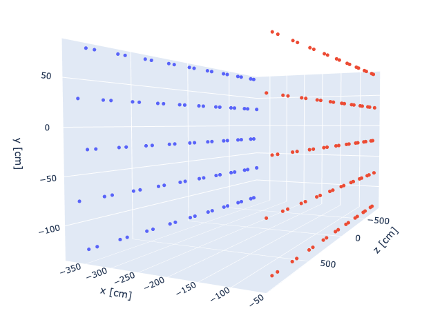
Figure 2: A module of the ICARUS detector. There are 180 PMTs mounted on the planes x = -59.36 mm (red) and -381.07 mm (blue), facing inwards to the detection volume.

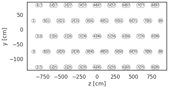
Figure 3: The locations of the first 90 PMTs at x = -381.07 mm of the ICARUS detector. The other 90 PMTs at x = -59.36 mm follow the same layout. Diameters of the PMTs are not drawn to scale.

A baseline SIREN model of $n_{L}=5$, $n_{F}=512$ and $\omega=30$ is trained on the simulated ICARUS detector in a batch size of 60676 voxels, corresponding to a total of 37 batches per epoch. Other choices of hyperparameters are discussed in Sec. IV.3. A weighting factor $w_{ij}\propto v_{ij}$ is included in the loss function $\mathcal{L}_{2}$ to account for the statistical uncertainty on the number of photons in the simulation. The training process takes about 30 minutes per 1000 epochs on a NVIDIA A100 GPU.

The SIREN model converges quickly to a relative bias of 10% within 200 epochs and plateaus at 7% (Fig. 4). As shown in Figures 5 and 6, this 7% comes mostly from regions with low visibility. For the bright regions with visibility greater than $10^{-3}$, the SIREN model reproduces the photon library within 1%. This is understood to be due to low statistics of detected photons in the simulation, as demonstrated in Section IV.2. Figure 7 shows a small varation of relative bias at $\pm 0.2\%$ depending on the PMT locations.

Figure 8 shows that the SIREN model reproduces the optical visibility map using a significantly smaller number of parameters ($\sim$1.4 million) than the lookup table approach ($\sim$404 million). Because of the differentiablity with respect to the input coordinates of the SIREN model, the gradient can be computed regardless of the grid resolution (Fig.9). The computation time and memory footprint of the SIREN model make it amenable to the computing resources of existing and future LArTPC experiments.

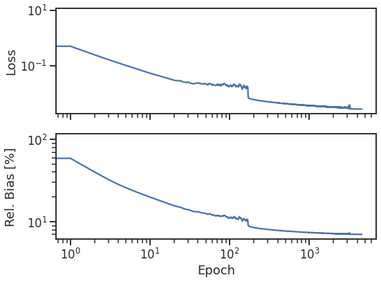
Figure 4: The loss (top) and relative bias (bottom) curves for training the baseline SIREN model with the ICARUS photon library.

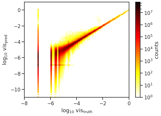
Figure 5: Predicted visibility from the baseline SIREN model v.s. the truth values from ICARUS photon library. Data points with zero visibility are put into the first non-empty bin.

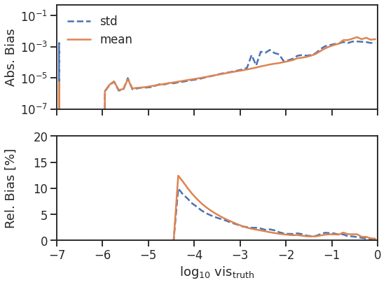
Figure 6: The mean (solid) and standard deviation (dashed) of the absolute (top) and relative (bottom) biases for the baseline SIREN model as a function of truth visibility from ICARUS photon library. Data points with zero visibility are put into the first empty bin.

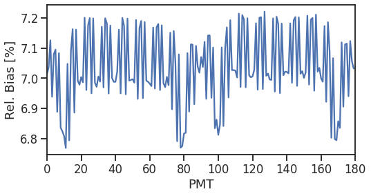
Figure 7: The relative bias of the baseline SIREN model, averaging over voxels, as a function of PMT indices. The variation of bias in PMTs is expected from the statistical unercainty of the simulation, as discussed in Section IV.2.

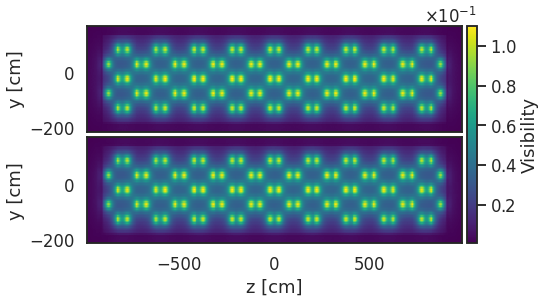
Figure 8: Sum of visibility for all PMTs at $x=-362.5~{}\mathrm{cm}$ from the photon library (top) and the SRIEN model (bottom).

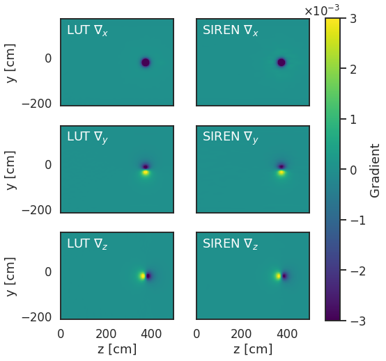
Figure 9: Gradients in $x$ (top), $y$ (middle) and $z$ (bottom) directions of PMT #63 at $x=-362.5~{}\mathrm{cm}$ from the photon library (left) and the SIREN model (right). The gradients of the photon libraray are estimated using Sobel filter Sobel (1968), while the gradients of the SIREN model are computed using PyTorch’s automatic differentiation engine Paszke et al. (2019).

IV.2 Statistical Uncertainty

A finite number of simulated photons is used for the construction of the photon library. There is therefore an inherent statistical limitation on the fidelity of the photon library, in particular for the dark regions of the detector, where very few photons are visible. As the photon library is used as the input for training the SIREN model, this inherent statistical uncertainty translates into an impact on the performance of the learned SIREN. To study this impact, a toy photon library is generated analytically as

$$\mathbf{\Psi}^{\mathrm{toy}}(\mathbf{x})=\max(ae^{-k\mathbf{r(\mathbf{x})}}/\mathbf{r(\mathbf{x})}^{2},1),$$ (7)

where $\mathbf{r}(\mathbf{x})$ is a vector of distances from the point $\mathbf{x}$ to the PMTs. This toy model includes the two most important features of the photon propagation, namely the inverse-square fall off away from the light source and the light attenuation in the transportation media. The constants $a=55$ and $k=0.006$ are chosen to loosely resemble the ICARUS photon library (Fig. 10). A noisy visibility lookup table is generated by

$$v_{ij}^{\mathrm{toy}}=\max\{\mathrm{Pois}(\mathbf{\Psi}^{\mathrm{toy}}_{j}(\mathbf{x}_{i})\times 10^{6})/10^{6},1\},$$ (8)

where $\mathrm{Pois}(\cdot)$ denotes a Poisson random variable. The toy+noise sample mimics the global features of the ICARUS photon library, which has an expected statistical uncertainty corresponding to $10^{6}$ generated photons per voxel (Fig. 10). The baseline SIREN training procedure is repeated for the toy model and toy+noise photon library. Similar to Fig. 4, the toy photon library with statistical uncertainty plateaus at 6.5% in relative bias, while the analytical toy model goes below 1% and still shows a downward trend after 10k epochs (Fig. 11). As shown in Fig. 12, the relative bias of the SIREN trained on the toy+noise sample follows the expected statistical error when compared to the toy+noise sample used for training, showing a similar trend as observed in Fig. 6.

On the other hand, the relative bias of the SIREN trained on the toy sample has very little dependence on the visibility at $\sim$1% (Fig. 12). By comparing the SIREN parameterization of the toy+noise sample to the toy model, the relative bias is similar to the SIREN model trained using toy model without statistical uncertainty. It indicates that the SIREN model is able to remove the statistical fluctuation from the photon library and learn the underlying distribution. It is therefore a more robust model of the visibility than the voxel representation, in addition to the other benefits as described above. The expected variation in bias due to statistical uncertainty from simulation is shown in Fig. 13. The performance of SIREN modeling of the ICARUS’s visibility LUT (Fig. 7) is dominated by the statistical fluctuation inheriting from the simulation.

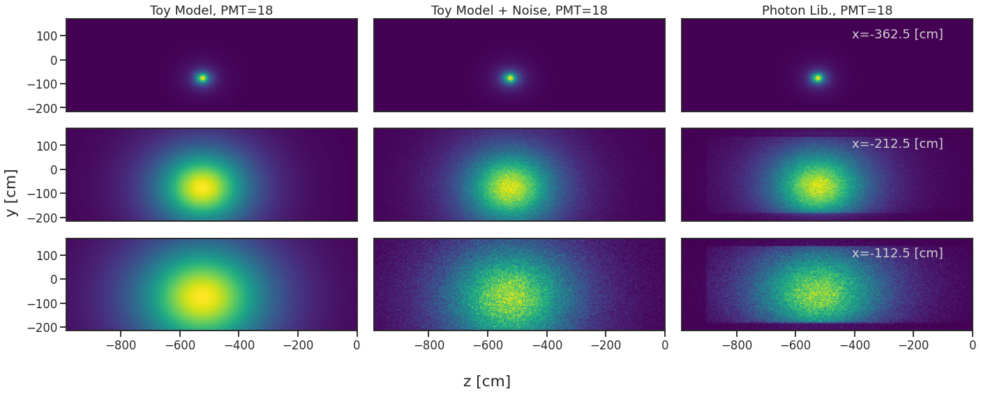
Figure 10: The visibility of PMT=18 at three different x positions for the toy model (left column), toy+noise sample (middle column) and the ICARUS photon library (right column).

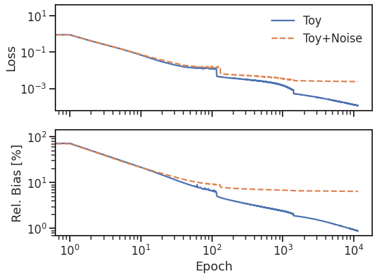
Figure 11: Training curves of the loss (top) and relative bias (bottom) for the toy model (solid) and the toy+noise sample (dashed).

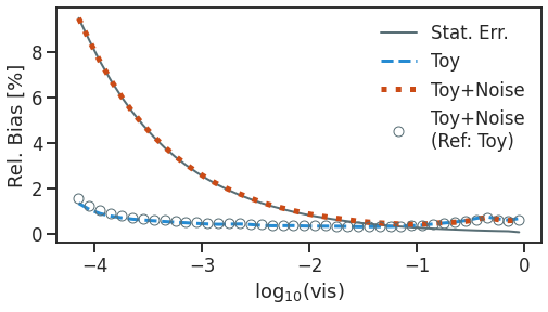
Figure 12: The relative bias for the analytical toy model (solid), toy+noise sample (red dotted) and expected statistical error (blue dashed) as a function of visibility. The data points (open circle) represents the SIREN model trained from the toy+noise sample with respect to the analytic toy model.

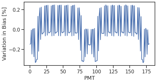
Figure 13: Expected variation in bias for different PMTs due to the statistical uncertainty from simulation.

IV.3 Hyperparameters

Different choices of hyperparameters are explored and compared to the baseline setting ($n_{L}=5,n_{F}=512,\omega=30$). Since the construction of SIREN from photon library is an overfitting problem, the accuracy will alwyas increase with the depth of the network and the number of hidden features. As shown in Fig. 14, the chosen baseline setting gives a bias that is consistent with the expected statistical uncertainty (Fig. 12). Adding one more layer ($n_{L}=6$) only gives a marginal improvement.

As shown in Fig. 15, the frequency factor $\omega$ has significant impact on the SIREN training time Sitzmann et al. . Without this multiplying factor ($\omega=1$), the convergence is much slower than with $\omega>1$. The choice of $\omega=30$ is optimal for the training. There is no further improvement with larger values.

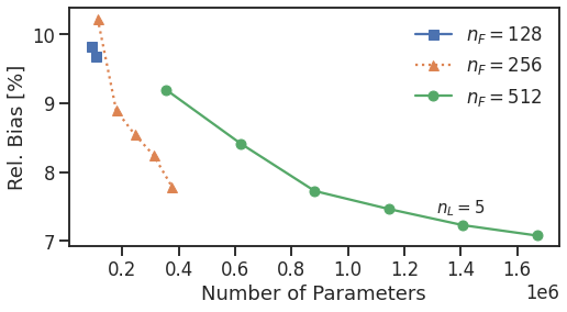
Figure 14: The best relative bias v.s. number of parameters for different SIREN hyperparameters of $n_{F}=128,~{}n_{L}=\{4,5\}$ (squares), $n_{F}=256,~{}n_{L}=\{1,2,3,4,5\}$ (triangles), and $n_{F}=512,~{}n_{L}=\{1,2,3,4,5\}$ (circles).

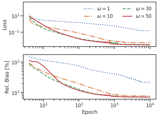
Figure 15: A study of hyperparameter $\omega$ for $n_{F}=512$ and $n_{L}=5$.

V Applications

V.1 Flash Matching

It is an intrinsic challenge to use only charge information from LArTPCs to determine the position of particles along the drift direction of the detector. Additional optical detectors (e.g PMTs) can detect scintillation light from particles in LArTPCs and provide timestamps of nanosecond precision, which can be used to accurately project the charge signals along the drift direction. The flash matching algorithm assumes a matched image pair from the charge readout and the PMT system. First, an offset $(x,y,z)\mapsto(x+x_{0},y,z)$ is applied along the drift direction for all of the voxels in the charge readout. Then the corresponding PMT readout given the charge signal is modeled using Eq. 5. The goal is to minimize $-\ln\mathcal{L}_{\mathrm{track}}$ for the offset $x_{0}$ using gradient descent , while keeping all other parameters fixed.

Traditionally the flash matching algorithm, as implemented by OpT0Finder, uses a C++ optimization library called MINUIT James (1998) . As an intermediate benchmark, we reimplemented the OpT0Finder algorithm in Python, and the MINUIT library is replaced by PyTorch’s automatic differentiation engine. Both the OpT0Finder and PyTorch methods use the lookup table as input, where the gradient is calculated from the grid values of the photon library using finite differences. The SIREN model is incorporated into the PyTorch implementation to replace the photon library, where the gradient of the visibilty is given by the derivative of the SIREN model.

A test sample of 10000 tracks in random locations and the corresponding photon detector output is generated according to Eq. 5 using the ICARUS photon library. The three flash matching algorithms are benchmarked with the track samples. As shown in Fig. 16, all three implementations give comparable results for the reconstruction of the absolute positions of the tracks and the number of photoelectrons of the PMTs. Though the performance is similar for all methods, the SIREN model is much more scalable than the lookup table approach, as it does not require grid-based calculation of the gradient.

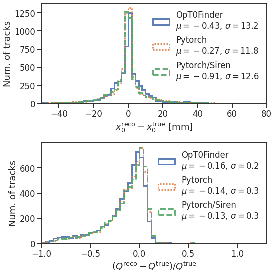
Figure 16: Benchmarks of the flash matching algorithm implemented in OpT0Finder, Pytorch and PyTorch+SIREN (see text for descriptions) in terms of reconstructed position (top) and reconstructed number of photoelectrons in PMTs (bottom).

V.2 Data-driven Calibration

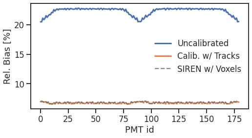
Figure 17: The relative bias of the modified photon library calculated using an uncalibrated SIREN model (blue). The calibrated SIREN model (orange) using 10000 tracks is consistent with re-training SIREN model with all the voxels from the modified photon library.

The SIREN models presented in Section III.1 are trained using a voxel-based loss to parametrize a fixed photon library lookup table. As this photon library is generated via detector simulation, a calibration procedure is required to correct for differences with respect to measured data. Because the learned SIREN model is fully differentiable, it may be automatically tuned to the data via a track-wise loss, as described in Section III.2, a notable advantage of the SIREN approach.

The calibration process follows a similar optimization procedure as the flash matching algorithm, where the goal again is to minimize $-\ln\mathcal{L}_{\mathrm{track}}$. However in this case, x0 is treated as fixed, and the SIREN parameters are optimized The assumption of known $x_{0}$ can be satisfied by selecting tracks crossing the physical boundaries of the detector.

A modified photon library is generated by multiplying $\exp(-kr(\mathbf{x}))$ to the original ICARUS photon library, where $r$ is the distance between position $\mathbf{x}$ and a PMT and $k=10^{-3}~{}\mathrm{cm}^{-1}$. The modified photon library has a maximum reduction of 85% in visibility and causes an average bias of 22.3% compared the SIREN model trained with the original ICARUS photon library (Fig. 17).

For the demonstration of the calibration process, a dataset of 10000 images of the photon detector are generated from simulating single track per image and the modified photon library according to Eq. 5. The track sample covers about one-third of the voxel space of the ICARUS detector volume. The SIREN model trained from the original ICARUS photon library is further fine-tuned with the track sample. As shown in Fig. 17, the calibrated SIREN model performs the same as if it was trained from scratch using the voxel-wise loss on the modified photon library.

VI Conclusion

We propose a new approach to parametrize LArTPC optical visibility using SIREN, a neural implicit representation with periodic activation functions. We demonstrate that this approach is able to reproduce the photon acceptance map with high accuracy, and further show that this approach is less sensitive to simulation statistics than commonly used lookup table methods. The number of parameters in our SIREN model is orders of magnitude smaller than the number of voxels in such lookup tables, making SIREN much more scalable to larger detectors. Furthermore, the SIREN model is easily tunable via automatic differentiation, and has well behaved derivatives due to its periodic activation functions. We demonstrate the potential of using these qualities to optimize SIREN directly on real data, an application which is infeasible with traditional approaches, mitigating the concern of data v.s. simulation discrepancies. We further present an application for data reconstruction where SIREN is used to form a likelihood function for photon statistics.

In summary, our method offers a pathway towards improving the physics quality of LArTPC simulation, while at the same time addressing issues of scalability which are essential problems for the future of LArTPC experiments. We note that this method is just one example of the power of differentiable surrogates in physics simulation, and we hope that it prompts ideas for the use of such methods in other areas of physics.

VII Acknowledgement

The authors wish to thank the ICARUS collaboration for providing access to the photon detector visibility lookup table upon which the results presented in Section IV are based. This work is supported by the U.S. Department of Energy, Office of Science, Office of High Energy Physics, and Early Career Research Program under Contract DE-AC02-76SF00515.

References

- (1) R. Acciarri et al., arXiv:1503.01520 .
- (2) A. Abud et al. (DUNE), arXiv:2103.13910 .
- Acciarri et al. (2017) R. Acciarri et al. (MicroBooNE), JINST 12, P02017 (2017).
- Dwyer et al. (2018) D. Dwyer, M. Garcia-Sciveres, D. Gnani, C. Grace, S. Kohn, M. Kramer, A. Krieger, C. Lin, K. Luk, P. Madigan, C. Marshall, H. Steiner, and T. Stezelberger, JINST 13, P10007 (2018).
- Rubbia et al. (2011) C. Rubbia et al. (ICARUS), JINST 6, P07011 (2011).
- Abi et al. (2020) B. Abi et al. (DUNE), JINST 15, T08010 (2020).
- (7) B. Mildenhall, P. P. Srinivasan, M. Tancik, J. T. Barron, R. Ramamoorthi, and R. Ng, arXiv:2003.08934 .
- (8) J. N. P. Martel, D. B. Lindell, C. Z. Lin, E. R. Chan, M. Monteiro, and G. Wetzstein, arXiv:2105.02788 .
- (9) V. Sitzmann, J. N. P. Martel, A. W. Bergman, D. B. Lindell, and G. Wetzstein, arXiv:2006.09661 .
- Cennini et al. (1995) P. Cennini, J. Revol, C. Rubbia, W. Tian, D. Dzialo Giudice, X. Li, S. Motto, P. Picchi, P. Boccaccio, F. Cavanna, et al., Nucl. Instr. and Meth. A 355, 660 (1995).
- Sorel (2014) M. Sorel, JINST 9, P10002 (2014).
- Sobel (1968) I. Sobel, Presentation at Stanford A.I. Project (1968).
- Paszke et al. (2019) A. Paszke, S. Gross, F. Massa, et al., in Advances in Neural Information Processing Systems 32 (Curran Associates, Inc., 2019) pp. 8024–8035.
- James (1998) F. James, “MINUIT: Function minimization and error analysis reference manual,” (1998).