Ryan Peterson1 and Joseph Cavanaugh2 Peterson and Cavanaugh Department of Biostatistics and Informatics, Colorado School of Public Health, University of Colorado - Anschutz Medical Campus, CO, USA Department of Biostatistics, College of Public Health, University of Iowa, IA, USA Ryan Peterson, Department of Biostatistics and Informatics, University of Colorado - Anschutz Medical Campus, 13001 E 17 Pl, Aurora, CO, 80045, USA ryan.a.peterson@cuanschutz.edu (+1) 303 724 0853 Fast, effective, and coherent time series modeling using the sparsity-ranked lasso Sparsity-ranked lasso for time series The sparsity-ranked lasso (SRL) has been developed for model selection and estimation in the presence of interactions and polynomials. The main tenet of the SRL is that an algorithm should be more skeptical of higher-order polynomials and interactions a priori compared to main effects, and hence the inclusion of these more complex terms should require a higher level of evidence. In time series, the same idea of ranked prior skepticism can be applied to the possibly seasonal autoregressive (AR) structure of the series during the model fitting process, becoming especially useful in settings with uncertain or multiple modes of seasonality. The SRL can naturally incorporate exogenous variables, with streamlined options for inference and/or feature selection. The fitting process is quick even for large series with a high-dimensional feature set. In this work, we discuss both the formulation of this procedure and the software we have developed for its implementation via the srlTS R package. We explore the performance of our SRL-based approach in a novel application involving the autoregressive modeling of hourly emergency room arrivals at the University of Iowa Hospitals and Clinics. We find that the SRL is considerably faster than its competitors, while producing more accurate predictions. autoregressive; exogenous covariates; forecasting; penalization; ranked sparsity; seasonality

1 Introduction

In time series analyses, the comfort of asymptopia, where our series of interest has infinite observations and can be suitably characterized by a small set of endogenous parameters, can become an entrapment. With freely available statistical and computational tools built for high dimensional problems, those who dare to venture away from conventional asymptotic theory may be able to build better predictive models and learn more richly about causal mechanisms at play in a data-saturated world.

In this work, we will show how new applications of existing statistical theories and tools can be utilized in time series analyses to produce better inferences and forecasts, focusing on scenarios with complex seasonal patterns and exogenous covariates. We start by describing the background and reviewing existing methods in this space, including common means of modeling seasonal time series data. We then illustrate how ranked-sparsity-based tools such as the sparsity-ranked lasso (SRL) can be extended to outperform existing methods, proceeding through both the formulation of the procedure and the software we have developed for its implementation via the srlTS R package. In our application, we explore the performance of our SRL-based approach relative to alternative methods on the autoregressive modeling of hourly emergency room visits at the University of Iowa Hospitals and Clinics (UIHC). We conclude with a discussion, including areas of future research.

2 Background

In this section, we will describe common models for seasonal time series data, several candidate fitting procedures, and several considerations in choosing parameters for these models.

2.1 Autoregressive Models

Consistent and continual data collection is beginning to pervade our lives in unprecedented and unexpected ways. Time series data, where one variable is measured many times at regular intervals, is ubiquitous. A measurement in the present usually depends on its past (say, $p$) values to some extent, and this dependence can be well captured by the autoregressive model. An autoregressive model of order $p$, or an AR($p$) model, can be written in a form analogous to a traditional regression model and estimated using standard ordinary least squares (OLS) techniques. The model has the structure

$$y_{t}=\beta_{0}+\beta_{1}y_{t-1}+...+\beta_{p}y_{t-p}+\varepsilon_{t}$$

where after controlling for the autocorrelation in the conditional mean structure, the residuals are assumed to be independent and normally distributed about zero.

One common question is the best way to select $p$ in the AR($p$) model in a given application – many techniques are possible, and some of the more common ones are outlined in the next section. Another related question is how to choose the “maximum $p$”; that is, the highest order $p$ that is considered in this model selection problem (we refer to this quantity as $p_{\max}$). Many times, $p$ is rather small, and selected on the basis of visual inspection of autocorrelation function (ACF) and partial autocorrelation function (PACF) plots which display autocorrelation and partial autocorrelation on lags up to $p_{\max}$. However, this technique is imperfect, as it injects human error and the potential for overfitting into the model selection process. Further, the need for visual inspection presents a barrier in higher dimensional settings where automated model selection methods are needed.

A time series may also be expected to follow some pattern of seasonality; for example, online searches related to the National Football League will peak during the football season every year. For this reason, it is important that this seasonality be specified in the autoregressive model. Let $\boldsymbol{\phi}$ refer to the local parameters and $\boldsymbol{\theta}$ refer to the seasonal parameters, and say (for now) that we know the periodicity of the seasonality is $m$ time measurements. The AR model can be written as

$$y_{t}=\beta_{0}+\sum_{j=1}^{p}\phi_{j}y_{t-j}+\sum_{j=1}^{P}\theta_{j}y_{t-jm}+\varepsilon_{t}$$

where again, the $\varepsilon_{t}$ are assumed to be independent and normally distributed conditional on the mean structure. As an illustrative example, if we consider a setting where the seasonal period is yearly, and the series is monthly, then $m=12$. If the series is weekly, then $m=52$, and so on. This AR model is referred as a seasonal autoregressive (SAR) model, and has parameter collections of size $p$ and $P$, which denote how many local and seasonal components are to be estimated, respectively. As with the standard AR model, model selection must take place in order to select $P\in\{0,1,2,...P_{\max}\}$.

The benefits of representing the AR and SAR models in this linear model form is that it becomes clear how least-squares (or some other estimation technique) can be used to estimate the AR parameters. However, there are also models that cannot be easily represented by this lagged model form – for instance, those with moving average (MA) components. The now-ubiquitous autoregressive integrated moving average (ARIMA) model can handle moving average terms as well as differencing, which may be advisable if the time series is not stationary (Cryer and Chan, 2008).

2.2 Existing Methods for Order Selection

For ARIMA models, it is common practice to use a likelihood-based estimation procedure to fit models with potentially both AR and MA terms. After a set of candidate models has been fit, an information criterion, such as Akaike’s Information Criterion (AIC), its small sample corrected version (AICc), or the Bayesian Information Criterion (BIC), can be used to select an optimal model order. This process is implemented automatically in the forecast package in R (Hyndman and Khandakar, 2008; Hyndman et al., 2018). In this framework, the candidate models can be fit either in a step-wise fashion or in a best-subsets fashion. In either case, we refer to this method as automated-ARIMA (AA).

If only AR and SAR models are considered, then the Least Absolute Shrinkage and Selection Operator (the lasso) (Tibshirani, 1996) can be used to estimate the coefficients and select an optimal $p$ and $P$ simultaneously. An important benefit to this approach is that the autoregressive components can be selected and estimated simultaneously alongside exogenous covariates. In the typical ARIMA selection framework, the need to select from a set of exogenous covariates (denoted by $X$) can complicate the model selection process considerably; neither step-wise selection nor best-subsets are feasible when the dimension of $X$ is large, when $p_{\max}$ is large, or when the sample size $n$ is massive.

When seasonality is suspected, many additional complications often arise. In the SAR model, we had to assume that $m$ was known and fixed, which also presumes that there are no missed measurements in the series. If either $m$ is unknown or variable, or the missingness has been accommodated by collapsing “gaps” in the series, all of the candidate SAR models will be misspecified to an uncertain extent. Unfortunately, in many circumstances, $m$ is neither fixed nor known; for instance if the series exhibits seasonality each month, the period must adjust to the different lengths of the months in a calendar year. In the AR framework, one potential solution is to include nearby seasonal lags as additional parameters:

$$y_{t}=\beta_{0}+\sum_{j=1}^{p}\phi_{j}y_{t-j}+\sum_{j=1}^{P}\boldsymbol{\theta}_{j}^{T}\boldsymbol{y}_{(t-jm-\epsilon):(t-jm+\epsilon)}+\varepsilon_{t}$$ (1)

Here, we employ the notation $\boldsymbol{y}_{a:b}^{T}=(y_{a},y_{a+1},...,y_{b-1},y_{b})$ to represent the full set of observations between time $a$ and time $b$, and $\boldsymbol{\theta}_{j}$ refers to the vector of length $2\epsilon$ of coefficients on lags near $t-jm$. In words, since it may be unknown which lags near $t-jm$ are important, this approach includes all the lags at or near $t-jm$ within $\epsilon$ that may be important in modeling $y_{t}$. Note that an AR($p$) model is achieved when $\boldsymbol{\theta}_{j}=\boldsymbol{0}\ \forall\ j$, and a SAR($P$) model is achieved if both $\epsilon=0$ and $\phi_{j}=0\ \forall\ j$.

If we use the lasso to fit this model, it will typically estimate some coefficients to be zero, so we can re-frame this selection problem, setting $p_{\max}=mP_{\max}+\epsilon\overset{\text{def}}{=}p^{*}$. When this simplifying assumption is incorporated into the framework, the seasonal AR model may be viewed as one of many candidates lasso models, and equation (1) simplifies to the potentially high-dimensional local AR model:

$$y_{t}=\beta_{0}+\beta_{1}y_{t-1}+...+\beta_{p^{*}}y_{t-p^{*}}$$ (2)

In words, instead of assuming there will be structural gaps in the important lags in the SAR model, we parametrize every coefficient up through the maximum possible lag and will take care (in the following section) to ensure the solution is sparse and resembles the SAR model. This formulation means that a very high order AR model could be selected, depending on the expected pattern of seasonality. However, if the primary goal is prediction in large-sample settings, there is no large downside to selecting a high order model (other than potentially adding in a lot of noise, which hopefully can be avoided with the use of the lasso and an effective model selection criterion).

It should be noted that if cross-validation (CV) is desired for any of the regularization-based approaches, the implementation of CV in the time series setting is inherently more complicated due to the dependence among observations. Left-out observations of $\boldsymbol{y}$ must pervade the entire model design matrix, and imputation must be done in order to fit the model appropriately. This procedure is beyond the scope of this manuscript. Thankfully, for our purposes, we can tune the lasso (and the SRL) models using either BIC or AICc. BIC will generally select sparser (lower order) autoregressive models, while AICc will attempt to minimize prediction error (typically by allowing more coefficients into the model).

Finally, another popular method for fitting seasonal time series with multiple modes of seasonality is called the TBATS method (which stands for “trigonometric, Box-Cox transform, ARMA errors, trend, and seasonal components”) (De Livera et al., 2011). As with automated-ARIMA, the TBATS method can be implemented efficiently in the forecast package, but importantly, this software does not allow for TBATS to be used in conjunction with exogenous variables. Further, the mode(s) of seasonality must be pre-specified in this framework.

3 Methods

In this section, we show how the SRL can be used in the time series regression framework to fit AR and SAR models quickly, effectively, and accurately, while also optionally accommodating and selecting from a set of important exogenous features.

3.1 Dynamic Penalty Tuning with the Sparsity-Ranked Lasso

When prior informational asymmetry is present among candidate predictors, for instance when selecting from all pairwise interactions and polynomials, Peterson and Cavanaugh (2022) motivated and explored the use of the sparsity-ranked lasso. Its main tenet is that an algorithm should be more skeptical of higher-order polynomials and interactions a priori compared to main effects, and hence the inclusion of these more complex terms should require a higher level of evidence. Otherwise, if interactions and polynomials are treated with “covariate equipoise”, algorithms will tend to yield many more false discoveries for interactions and polynomials, which makes models less transparent, harder to communicate, and worse at prediction. The intuition behind the lasso-based implementation of ranked sparsity (the SRL) involves assigning weights to each candidate covariate based on the degree of skepticism that the covariate should in fact enter the model, as illustrated in the expression below.

$$\left|\left|\boldsymbol{y}-X\boldsymbol{\beta}\right|\right|^{2}+\lambda\sum_{j=1}^{k}w_{j}|\beta_{j}|$$

Here, $k$ refers to the column dimension of the matrix of covariates $X$. The addition of the $w_{j}$ is the only difference between this formulation and the traditional lasso (Tibshirani, 1996), and while the adaptive lasso (which shares the same representation) fixes the $w_{j}$ values in a way that corresponds to a data-based “first glance” (Zou, 2006), the SRL sets these weights based on a prior degree of skepticism related to each covariate. While the intuition behind these weights appears to be quite subjective for the SRL, in its motivation, the authors justified several objective ways of characterizing this skepticism in the context of interactions and polynomials. This concept can be extended to selecting features in a time series regression framework, which we describe in this section.

The SRL is designed to be of use when the assumption of covariate equipoise, defined as the prior belief that all covariates are equally worthy of entering into the model, is not satisfied. In the AR framework, this assumption is definitely not satisfied, and the SRL can address the resulting challenge. Particularly, going from equation (1) to equation (2) in the previous section is suspect; we have very good reason to believe that the effects on the lags between $p$ and $m-\epsilon$ are equal to zero. We are also much more inclined to think that more recent lags are more likely to be important a priori than lags representing the more distant past. If $m$ is known, we are much more willing to believe the $m$th lag to be predictive than other periodic lags. The SRL can accommodate such expected differences in skepticism by scaling the penalty differently for different lags in the model. In this subsection, we discuss two methods for adapting the SRL to handle time series data: we can either parametrize skepticism, or we can use the data to inform it.

Parameterizing skepticism

Since we have good reason to believe that recent and seasonal lags are more likely to be important, but we are not certain, we can operationalize this notion using what we call penalty-scaling functions. These penalty-scaling functions, which we denote as $f$, provide ways of informing the weight of the lasso penalty $w_{j}$ that corresponds to the $j$th lag, i.e. $w_{j}=f(j,\cdot)$. We discuss two different penalty-scaling functions: one that relates to a lag’s “locality” (i.e. its recency), and one that relates to its season. We also show how combinations of these two penalty-scaling functions can be utilized in a manner that is both flexible and widely applicable. For locality, we use $\gamma_{l}$ to illustrate the strength of this scaling factor, which is treated as a tuning parameter. For $\gamma_{l}\geq 0$, and for a coefficient on the $j$th lag of $y_{t}$, we define the local penalty-scaling function as

$$f_{l}(j,\gamma_{l})=(j/p^{*}+c)^{\gamma_{l}}=\exp\left\{\gamma_{l}\log(j/p^{*}+c)\right\}$$

If $\gamma_{l}=0$, the resulting procedure is equivalent to the ordinary lasso, since the function evaluates to 1 $\forall\ j$. The addition and the choice of the constant $c$ is somewhat arbitrary. If $c=.5$, this ensures that the scaling factor evaluates to 1 at the middle lag considered, $p^{*}/2$. This choice of $c$ effectively relaxes the original lasso’s penalty for early lags, and increases it for later lags. One could also set $c=1$ instead, which would simply increase the penalty for all lags instead of having the relaxing property. In practice, since one has to tune the original lasso penalty $\lambda$ anyway, the choice of $c$ typically makes little to no difference. This function is visualized with $c=.5$ for various $\gamma_{l}$ in the top plot of Figure 1 for all lags up to $p^{*}$.

For the seasonal penalty-scaling function, we use the parameter $\gamma_{s}$ to represent the strength of the penalty scaling function. For $\gamma_{s}\geq 0$, the proposed penalty scaling function for the $j$th lag is

$$f_{s}(j,\gamma_{s},m)=\exp\left\{\gamma_{s}\left[-\cos\left(\frac{2\pi*j}{m}\right)\right]\right\}$$

Here $m$ is the (suspected) seasonal frequency, which is set to 52 in the visualization in the middle plot of Figure 1. Similar to the locality function, setting $\gamma_{s}$ to 0 yields the ordinary lasso. Finally, we can combine the two penalty-scaling functions by simply multiplying $f_{l}$ and $f_{s}$ together. For $\gamma_{l}\geq 0,\gamma_{s}\geq 0$, we have

$$f_{as}(j,\gamma_{s},\gamma_{l},m) =\exp\left\{\gamma_{s}\left[-\cos\left(\frac{2\pi*j}{m}\right)\right]\right\}*(j/p^{*}+c)^{\gamma_{l}}$$

$$=\exp\left\{\gamma_{s}\left[-\cos\left(\frac{2\pi*j}{m}\right)\right]+{\gamma_{l}}\log(j/p^{*}+c)\right\}$$

This penalization is visualized for different values of $\gamma_{l}$, $\gamma_{s}$, and $j$ in the bottom plot of Figure 1.

The parametrically-weighted SRL method is not without drawbacks. For instance, if $m$ is completely unknown ahead of time, one cannot parametrize the seasonal scaling function correctly, and it also becomes unclear how to best select $p^{*}$. Another minor drawback occurs when the seasonal frequency $m$ is known exactly (without multiple modes), in which case the algorithm may select lags close to $m$ instead of the “true” model with only the $m^{th}$ lag included (e.g. for simulated SAR(1) series). SRL penalizes the lag-$m$ coefficient very similarly to those surrounding $m$, and the lasso is prone to select from correlated variables somewhat arbitrarily. Finally, the combined penalty scaling function is not always defensible; the period of the wave depends (to a small degree) on the locality hyperparameter, and therefore the two $\gamma$ parameters interfere with each other. This can lead to issues of identifiability; we have found in practice that the optimal solution using this technique, as measured by an information criterion, can lie on a line of $\gamma_{l},\gamma_{s}$ tuning parameters, although this line often does not intersect with the lasso solution (where both $\gamma_{l}=0$ and $\gamma_{s}=0$).

We have explored these parametrized penalty-scaling functions and applied them successfully in multiple applications. However, we omit these results for the sake of brevity, and because the SRL method that we discuss in the next subsection performs similarly and is more broadly applicable than the parametrized version.

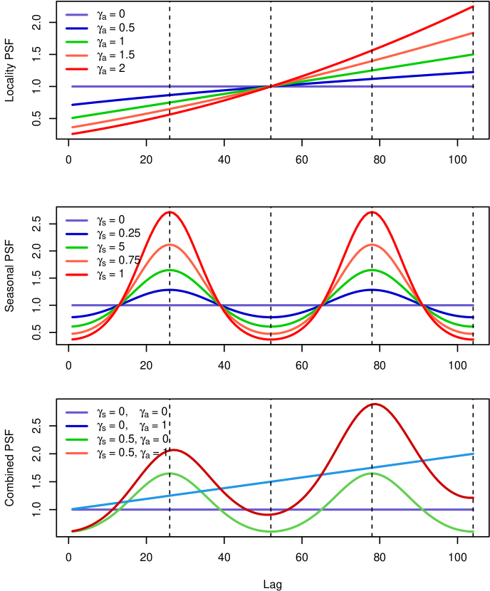
Figure 1: Parametrized penalty scaling functions (PSF) for coefficients on lags up to $p^{*}$ in a time series SRL setting. The top plot refers to the locality PSF ($c=.5$), the middle plot refers to the seasonal PSF, and the bottom plot is their combined PSF. In the bottom plot, $c=1$.

SRL with the Partial Autocorrelation Function

Instead of having a predefined parametrized ranking of skepticism for various lags in a time series model, we could use the data to inform these penalty weights. A useful means to accomplish this is to use the partial autocorrelation function (PACF), defined as the correlation between $y_{t}$ and $y_{t-k}$ after removing the effect of the intervening variables $y_{t-1},y_{t-2},...,y_{t-k+1}$. The PACF is easy to calculate, and it provides a data-driven measure of the importance of each lag – many statistical practitioners inspect the PACF to determine which lags should be considered and estimated in an autoregressive model (Cryer and Chan, 2008).

The adaptive lasso (Zou, 2006) involves penalty weights $w_{j}$ that are informed by an initial “first-stage” estimate of $\boldsymbol{\beta}$, often accomplished via a simple OLS estimate. In our case, we suggest using PACF estimates instead by setting

$$w_{j}=\left(\frac{1}{|\hat{\phi}_{j}|}\right)^{\gamma}$$

Here $\hat{\phi}_{j}$ represents the estimated PACF on the $j$th lag of $y_{t}$. Each of these estimates is equivalent to the $j^{th}$ AR coefficient estimate in an AR($j$) model, and can therefore be obtained via a heuristically-guided solution path from an AR(1) to an AR($p^{*}$). In words, $\phi_{j}$ measures the relative importance of the $j^{th}$ lag, conditional on all of the more recent lags. Penalty weights estimated with such an approach will tend to be smaller for more recent lags compared to those based on the full AR($p^{*}$) model. Penalty weights estimated using the AR($p^{*}$) model do not seem to perform as well (results not shown). We refer to this approach as the SRLPAC (sparsity-ranked lasso with partial autocorrelation) procedure, pronounced “SRL-pack”.

If there are exogenous covariates, we can include weights for these as well; let $\boldsymbol{w}_{endo}$ refer to the vector of weights on endogenous features (i.e., the lags of $\boldsymbol{y}$), and $\boldsymbol{w}_{exo}$ refer to that for a set of exogenous features in a $n\text{ x }k$ model matrix $X$. The latter exogenous weights can be applied set to the marginal OLS estimates or the OLS estimates controlling for the autocorrelation in the series in a similar adaptive lasso fashion. This approach will share similar properties to the adaptive lasso, and will therefore be useful and computationally feasible even with high dimensional (high $k$) feature sets. However, estimation shrinkage complicates formal statistical inference on coefficients. Alternatively, if $\boldsymbol{w}_{exo}$ is set to $\boldsymbol{0}$, then the coefficients on exogenous features are unpenalized, and formal means of statistical inference on them is possible via ordinary least squares using the penalized linear predictors from the endogenous features as an offset. Regardless of the weights chosen, we refer to this approach as the SRLPACx procedure, pronounced “SRL-packs,” in a similar spirit as ARIMAX which also allows for exogenous variables.

The SRLPAC approach is ideal for modeling time series data with complicated seasonality; it is quick, intuitive, and can be conveniently tuned using AICc or BIC provided the sample size is large, which is typically the case in time series settings. Further, SRLPAC does not require the pre-specification of seasonal modes at all; it does this naturally and automatically using the PACF. Finally, the SRLPACx approach has all the same advantages while also allowing for seamless integration of (possibly very many) exogenous variables.

3.2 Measuring Predictive Accuracy

In order to measure prediction accuracy in a time series setting, there are many possible options. We utilize several different methods, each of which is focused on the predictive accuracy of the models in forecasting new data. We use the root-mean-squared prediction error (RMSPE), $R^{2}$, the mean absolute error (MAE), and the mean absolute percentage error (MAPE) (Hyndman, 2006). These metrics are all estimated using out-of-sample data, and are subsequently defined in this section.

For a set of predicted values $\hat{\boldsymbol{y}}^{*}$, and a set of $n^{*}$ out-of-sample observations that were not used in calculating these predictions, $\boldsymbol{y}^{*}$, we define RMSPE as

$$\text{RMSPE}=\sqrt{\frac{1}{n^{*}}\sum_{i=1}^{n^{*}}(\hat{y}_{i}^{*}-y_{i}^{*})^{2}}$$

RMSPE is interpretable in the same unit of measurement as the original measurement for $y$, and it signifies how far away from the true value our predictions were, on average. Another measure $R^{2}$, is defined as

$$R^{2}=1-\frac{\sum_{i=1}^{n^{*}}(\hat{y}_{i}^{*}-y_{i}^{*})^{2}}{\sum_{i=1}^{n^{*}}(y_{i}^{*}-\bar{y}^{*})^{2}}$$

This definition of $R^{2}$ differs slightly from other definitions in that there is no guarantee that it be non-negative, as is the case for $R^{2}$ in its typical in-sample setting. As a result, this version of $R^{2}$ does not have quite as clean of an interpretation. However, values close to 1 indicate very accurate predictions relative to naively guessing the mean, and values close to 0 indicate that using the mean of the responses for forecasting would have done as well as the model-based predicted values. Negative values indicate that the model-based predictions actually performed worse than the mean.

Since the RMSPE metric is not robust to outliers, another commonly used metric is the mean absolute error, defined here as

$${\text{MAE}}=\frac{1}{n^{*}}\sum_{i=1}^{n^{*}}|\hat{y}_{i}^{*}-y_{i}^{*}|$$

The interpretation of this measure is very similar to RMSPE. A related metric is the mean absolute percentage error, which is defined as

$${\text{MAPE}}=\frac{100}{n^{*}}\sum_{i=1}^{n^{*}}\frac{|\hat{y}_{i}^{*}-y_{i}^{*}|}{y_{i}^{*}}$$

The scaling of the summed errors by the value of $y_{i}^{*}$ and its multiplication by 100 entail that the MAPE has a percentage interpretation: how far off, in terms of a percentage, can we expect our predictions to be from the true value, on average? In this formulation, the denominator is often replaced with $\bar{y}_{i}^{*}$ to account for zero values (a convention we follow in the subsequent sections).

3.3 The srlTS package

We have developed the srlTS package in the R statistical software to implement the novel methods described previously. Using the slrTS function, a user must only supply the time series of interest as the outcome, and can optionally supply additional components which include: a matrix of exogenous features, the maximum lag considered ($p_{\max}$), a vector of weights for the endogenous features ($\boldsymbol{w}_{endo}$), a vector of weights for the exogenous features ($\boldsymbol{w}_{exo}$), a vector of candidate exponents for the penalty weights ($\gamma$), a proportion to use for the training of the model if out-of-sample prediction accuracy is of interest, and several other minor components (see package documentation). The penalty weights refer to the inverse of the penalty factors in the SRL fitting procedure such that a coefficient with a weight of 0 will have zero chance of entering the model, and a weight of $\infty$ will be unpenalized. An appealing property that results from setting weights to $\infty$, especially for exogenous features, is that statistical inference can be conducted using traditional methods without correcting for post-selection inference or accounting for bias due to the shrinkage of the coefficient. For this reason, the default option for $\boldsymbol{w}_{exo}$ is “unpenalized”, so that coefficients and standard errors are easily estimated and unbiased (via the summary function). The fitting engine for the lasso is accomplished via the ncvreg package (Breheny and Huang, 2011) which uses coordinate descent, and allows for additional features such as nonconvex penalization, an L2 penalty parameter which allows for the elastic net, and non-normally distributed outcomes. Model fitting involves two tuning parameters, $\lambda$ (the extent of overall coefficient penalization) and $\gamma$ (the degree of emphasis placed on the penalty weights), as defined previously. By default the srlTS function will use the AICc to select the best values, starting with $\gamma\in\left\{0,0.25,0.5,1,2,4,16\right\}$ and running each of these through 101 decreasing values of $\lambda$ according to the standard limits implemented in ncvreg. BIC is also available as an alternate means of tuning parameter selection.

The srlTS package is currently available on GitHub with a planned release to the Comprehensive R Archive Network upon acceptance of this manuscript. A tutorial on several popular time series data sets is included in the package website as a vignette, as well as a more in-depth vignette which more completely describes the programmatic details of the SRLPAC detailed in the forthcoming application.

4 Application – Emergency Room Visits

SRLPAC is able to shine especially when there are multiple modes of seasonality. In this application, we showcase some of these benefits in a novel approach to emergency room visit forecasting. For planning purposes, it is highly desirable to accurately forecast the expected number of visits in the emergency room (ER) each hour. Accurate forecasting (and planning) reduces the costs and frustrations associated with having to “call-in” extra help. Previous research has indicated that time series models can be developed and utilized to predict ER visits on the daily time-horizon (Jones et al., 2008). However, these daily forecasts, while informative, are less helpful from a practical standpoint since shifts are typically set for under 12 hours. It is useful to have more granular predictions so that personnel resources can be allocated more efficiently on a shift-by-shift basis. Other research investigating the forecasting of ER arrivals at the hourly level does exist, and mostly utilize seasonal ARIMA models to fit the hourly series for a single ER. A detailed literature review is outside the scope of this manuscript.

In this study, we examine hourly visit counts for the Emergency Department at the University of Iowa Hospital and Clinics (UIHC) from July 2013 to March 2018. Since this is hourly data over a long time span, the sample size in this modeling problem is large ($n=41,640$). Further, multiple modes of seasonality are feasible; we expect to see more visits during the day than at night, and there could be weekly and monthly periodicities as well. The high sample size also yields minor computational concerns for some of the methods we have described.

The PACF is shown in Figure 2; we see that there are indeed many modes of seasonality. The most prominent correlation is the AR(1) term, but there are also large spikes around 23 hours, 47 hours, 72 hours, 7 days, 14 days, 21 days, and 28 days. Curiously there does not seem to be a prominent month effect around the 30-day mark.

Figure 2: PACF for 840 lags of hourly visits to the emergency room.

While many exogenous variables could feasibly factor into the number of emergency room visits in an hour, for the sake of this problem, we limit our consideration to monthly fixed effects, holiday effects, and concurrent hourly temperature in Iowa City, IA, as exogenous features (which are unpenalized in the regression). For holidays, we included separate fixed effects (as indicators) on Christmas, New Year’s Eve, New Year’s Day, Thanksgiving, Independence Day, and Hawkeye game-day (i.e., the day of an Iowa Hawkeye college football game). We also include holiday “plus-one” effects for Christmas and Thanksgiving to examine if there are lingering effects of these major holidays.

Before fitting the models, we divide our sample into a training set (the first 90% of data, 7/1/2013 until noon 10/9/2017) and a test set (the final 10% of data, starting noon 10/09/2017 to 3/31/2018). Using the training set, we fit the following models:

1. SRLPAC

2. SRLPAC with exogenous variables (SRLPACx)

3. Automated seasonal ARIMA (auto-SARIMA) selected using AICc. Note that for the auto-SARIMA approach, only one mode can be supplied, so we specified a daily frequency ($m=24$) for this setting based on the PACF plot.

4. TBATS model with mid-day, daily, weekly, and monthly frequencies specified: $m=(12,24,168,672)$.

After fitting these models, we then investigate the metrics outlined in the previous section. We repeat the fitting process 12 times to calculate the mean computation time (MCT) for each method in minutes. For both SRLPAC models, we use AICc to select a value of $\lambda$ and $\gamma$. For the SRLPACx model, we interpret terms in context as well as 95% confidence intervals based on OLS models where the penalized linear predictors are included as an offset. Finally, for staffing purposes, it is arguably more informative to investigate how well the model performs at predicting the number of visits that occur in a given 8-12 hour window, rather than at the hourly level. So, we also investigate the performance of the SRL and TBATS methods in predicting the 10-hour rolling sum of patients, which was calculated using the sum of the 1- through 10-step-ahead predictions on the test data set.

Table 1: Model performance for hourly arrivals. Prediction metrics were estimated using a left-out test sample, and the mean computation time (MCT) in minutes was computed across 12 replications on a single core of a machine running Mac OS.

	$R^{2}$	RMSPE	MAE	MAPE	MCT (Minutes)
SRLPAC	0.528	2.651	2.051	31.3	0.85
SRLPACx	0.530	2.645	2.045	31.2	1.09
Auto-SARIMA	0.373	3.053	2.353	35.9	6.42
TBATS	0.520	2.672	2.075	31.7	8.50

Results

We see in Table 1 that the auto-SARIMA approach performed the worst by all measures; it took a relatively long time to run, and the models it produced did not predict accurately. The TBATS method did predict quite well, though it also took much longer to run than either SRLPAC approach. SRLPAC and SRLPACx performed admirably, both with and without the exogenous variables, the inclusion of which seems to offer a modest improvement in predictive accuracy. The best predicting model was the SRL with exogenous variables. In this optimal model, the estimated coefficients for the exogenous variables are shown in Figure 3 as well as summarized in Table 2.

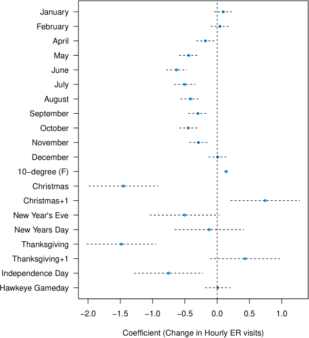
Figure 3: Coefficient estimates and 95% confidence intervals for exogenous variables in SRLPAC model. Values refer to the expected change in hourly visits controlling for other factors in the model, including the temporal correlation among observations.

Hourly ER visits do seem to exhibit seasonality on a yearly-scale, controlling for the rest of the covariates in the model. Specifically, there were fewer patients per hour in the summer than in the winter. It is important to realize, however, that we are controlling for the hourly concurrent mean temperature in the model as well, which has a very strong positive association with patient arrivals. For every 10 degree F increase in temperature, we expect to see about 0.14 more patients per hour, controlling for the month and holiday effects. We observe very strong negative effects on the major holidays, most of all Christmas and Thanksgiving on which there were about 1.5 fewer patients per hour, on average. This effect seems to have consequences; on the day after Christmas and Thanksgiving, there are about 0.74 and 0.43 more patients per hour, respectively. The effects of New Year’s Eve, New Year’s Day, and Independence Day are all negative, but are less pronounced than Christmas and Thanksgiving. There does not seem to be a large change in the number of patients per hour on Hawkeye game-days. Note that each interpretation of these fixed effects is also controlling for the “important” local and periodic autocorrelation in the series by the nature of the SRLPAC approach.

Table 2: Estimated coefficients and confidence intervals for the SRLPACx – AICc model.

	Coefficient	95% CI
Monthly Fixed Effects
January	0.094	(-0.05, 0.23)
February	0.043	(-0.10, 0.18)
March	Baseline
April	-0.182	(-0.32, -0.04)
May	-0.441	(-0.59, -0.30)
June	-0.628	(-0.79, -0.47)
July	-0.503	(-0.67, -0.34)
August	-0.411	(-0.57, -0.26)
September	-0.296	(-0.44, -0.15)
October	-0.447	(-0.58, -0.31)
November	-0.289	(-0.43, -0.15)
December	0.007	(-0.13, 0.15)
Other Effects
10°F Increase	0.142	(0.12, 0.17)
Christmas	-1.452	(-1.99, -0.92)
Christmas+1	0.744	(0.21, 1.28)
New Year’s Eve	-0.506	(-1.04, 0.03)
New Years Day	-0.122	(-0.66, 0.41)
Thanksgiving	-1.482	(-2.02, -0.95)
Thanksgiving+1	0.432	(-0.11, 0.97)
Independence Day	-0.752	(-1.29, -0.22)
Hawkeye Gameday	0.009	(-0.19, 0.20)

Table 3 shows how well each model predicted how many patients arrived in the ER in a 10-hour window. The SRLPAC methods performed similarly to one another with a slight advantage toward the SRLPACx model. This optimal model was able to describe 85.4% of the variation in the 10-hour rolling sum of ED arrivals. The SRLPACx model’s MAE was the lowest; its prediction was on average only about 6.8 patients off of the true value. Finally, Figure 4 shows the accuracy of the SRLPACx model in predicting the 10-hour rolling counts. Of note, the SRLPAC and SRLPACx models generated 1- through 10-step ahead predictions in under 5 minutes, while TBATS and SARIMA procedures took considerably longer (2 hours for the TBATS predictions and over 6 days for the SARIMA predictions).

Table 3: Model prediction performance for 10-hour rolling sum of patient arrivals.

	$R^{2}$	RMSPE	MAE	MAPE
SRLPAC	0.839	9.004	7.088	10.8
SRLPACx	0.854	8.564	6.787	10.4
Auto-SARIMA	0.761	10.997	8.683	13.3
TBATS	0.824	9.434	7.411	11.3

Figure 4: Absolute vs. predicted values for 10-hour patient arrival counts for SRLPACx model tuned with AICc. The dotted line is where $y=x$.

5 Discussion

We have shown that the SRL is adaptable to time series data in several ways. Not only does the SRLPAC method rival the prediction accuracy of other state-of-the-art forecasting methods, it is able to incorporate exogenous data seamlessly and run considerably faster for large data sets. Using the model fit with SRLPAC, we were able to accurately forecast the number of patients who would arrive at the UIHC Emergency Department to within an average of about 7 patients per 10-hour time window. We were also able to use the SRLPACx model to make inferences about patterns in the data, finding large correlations between ER arrivals and temperature, month, and holidays.

Many researchers have shown that SARIMA models are effective in forecasting the number of ER arrivals at other institutions. However, we have shown that at least for the UIHC Emergency Department, the SARIMA model does not perform effectively compared to other methods. In future work, we will compare the SRLPAC approach to other popular forecasting methods in this domain, which include SARIMAX (SARIMA with exogenous variables) and neural networks. We will also investigate model averaging approaches which blend multiple values of the tuning parameters of SRLPAC ($\gamma$ and $\lambda$) based on their likelihoods to provide a potentially more accurate prediction.

References

- Breheny and Huang (2011) Breheny, P. and Huang, J. (2011). Coordinate descent algorithms for nonconvex penalized regression, with applications to biological feature selection. Annals of Applied Statistics, 5(1), 232–253.
- Cryer and Chan (2008) Cryer, J. D. and Chan, K.-S. (2008). Time Series Analysis with Applications in R. Springer.
- De Livera et al. (2011) De Livera, A. M., Hyndman, R. J., and Snyder, R. D. (2011). Forecasting time series with complex seasonal patterns using exponential smoothing. Journal of the American Statistical Association, 106(496), 1513–1527.
- Hyndman et al. (2018) Hyndman, R., Athanasopoulos, G., Bergmeir, C., Caceres, G., Chhay, L., O’Hara-Wild, M., Petropoulos, F., Razbash, S., Wang, E., and Yasmeen, F. (2018). forecast: Forecasting functions for time series and linear models. URL http://pkg.robjhyndman.com/forecast. R package version 8.4.
- Hyndman (2006) Hyndman, R. J. (2006). Another look at forecast-accuracy metrics for intermittent demand. Foresight: The International Journal of Applied Forecasting, 4(4), 43–46.
- Hyndman and Khandakar (2008) Hyndman, R. J. and Khandakar, Y. (2008). Automatic time series forecasting: the forecast package for R. Journal of Statistical Software, 26(3), 1–22. URL http://www.jstatsoft.org/article/view/v027i03.
- Jones et al. (2008) Jones, S. S., Thomas, A., Evans, R. S., Welch, S. J., Haug, P. J., and Snow, G. L. (2008). Forecasting daily patient volumes in the emergency department. Academic Emergency Medicine, 15(2), 159–170.
- Peterson and Cavanaugh (2022) Peterson, R. A. and Cavanaugh, J. E. (2022). Ranked sparsity: A cogent regularization framework for selecting and estimating feature interactions and polynomials. AStA Advances in Statistical Analysis, 106, 427–454. 10.1007/s10182-021-00431-7.
- Tibshirani (1996) Tibshirani, R. (1996). Regression shrinkage and selection via the lasso. Journal of the Royal Statistical Society: Series B, 58(1), 267–288. ISSN 00359246. URL http://www.jstor.org/stable/2346178.
- Zou (2006) Zou, H. (2006). The adaptive lasso and its oracle properties. Journal of the American Statistical Association, 101(476), 1418–1429. 10.1198/016214506000000735. URL https://doi.org/10.1198/016214506000000735.