Deep Learning Hamiltonians from Disordered Image Data in Quantum Materials

Abstract

The capabilities of image probe experiments are rapidly expanding, providing new information about quantum materials on unprecedented length and time scales. Many such materials feature inhomogeneous electronic properties with intricate pattern formation on the observable surface. This rich spatial structure contains information about interactions, dimensionality, and disorder – a spatial encoding of the Hamiltonian driving the pattern formation. Image recognition techniques from machine learning are an excellent tool for interpreting information encoded in the spatial relationships in such images. Here, we develop a deep learning framework for using the rich information available in these spatial correlations in order to discover the underlying Hamiltonian driving the patterns. We first vet the method on a known case, scanning near-field optical microscopy on a thin film of VO₂. We then apply our trained convolutional neural network architecture to new optical microscope images of a different VO₂ film as it goes through the metal-insulator transition. We find that a two-dimensional Hamiltonian with both interactions and random field disorder is required to explain the intricate, fractal intertwining of metal and insulator domains during the transition. This detailed knowledge about the underlying Hamiltonian paves the way to using the model to control the pattern formation via, e.g., tailored hysteresis protocols. We also introduce a distribution-based confidence measure on the results of a multi-label classifier, which does not rely on adversarial training. In addition, we propose a new machine learning based criterion for diagnosing a physical system’s proximity to criticality.

I Introduction

The types of surface probes, such as atomic force microscopy (AFM), scanning tunneling microscopy (STM), and scattering scanning near-field infrared Microscope (SNIM), among many others Basov et al. (2011); Binnig and Rohrer (1999) and the wealth of data they generate is increasing at a rapid pace. As often happens in science, new experimental frontiers reveal new physics: These scanning and image probe experiments often reveal complex electronic pattern formation spanning multiple length scales at the surface of correlated quantum materials, even when they are atomicaly smooth.Qazilbash et al. (2007); Kohsaka et al. (2007); Guénon et al. (2013); Lange et al. (2021); Phillabaum (2012); Liu et al. (2016a); Dagotto (2005); Moreo et al. (2000); Cho et al. (2019); Battisti et al. (2016a, b) For example, manganites can have ferromagnetic and antiferromagnetic regions that coexist on multiple length scales.Dagotto (2005) In the unidirectional electronic glass in cuprates,Kohsaka et al. (2007) domains of stripe orientation take fractal form with correlations over 4 orders of magnitude in length scale.Phillabaum et al. (2012a) Magnetic domains in NdNiO₃ were also revealed to have fractal textures.Li et al. (2019a) We focus here on VO₂, a material whose metal and insulator domains can show self-similar structure over multiple length scales.Qazilbash et al. (2007); Liu et al. (2016a); Sharoni et al. (2008)

Unfortunately, most of our theoretical tools are designed for understanding and describing homogeneous electronic states. Therefore it is vital that we envision new theoretical frameworks for understanding why the patterns form in strongly correlated materials. The cluster analysis techniques we developed for interpreting these images have already uncovered universal behavior among disparate quantum materials,Qazilbash et al. (2007); Post et al. (2018); Li et al. (2019a); Phillabaum (2012); Liu et al. (2016a) but the methods only work on systems near criticality, and for sufficiently large fields of view. Powerful image recognition methods from machine learning (ML) hold potential to complement and extend these analyses into new regimes.

There has been tremendous growth recently in the application of ML methods to condensed matter. (For reviews, see Refs. Carleo et al., 2019; Carrasquilla, 2020; Bedolla et al., 2021; Mehta et al., 2019.) ML is being applied as a tool to tackle various problems in condensed matter physics, including disordered and glassy systems systemsRonhovde et al. (2011); Schoenholz et al. (2016); Arsenault et al. (2014), quantum many body problemsCarleo and Troyer (2016), quantum transportLopez-Bezanilla and Lilienfeld (2014), renormalization groupMehta and Schwab (2014); Beny (2013), and big data in materials scienceSchmidt et al. (2019); Ghiringhelli et al. (2015). ML also benefits from physics, an area known as physics-inspired ML theory.Carleo et al. (2019) Applied to experimental data, ML has been used to detect which phase of matter a physical system is in,Zhang et al. (2019) and aid in the experimental detection of the glass transition temperature.Zhang and Xu (2020) Other common uses of ML for experimental data include the extraction of material parameters from experiment, Schmidt et al. (2019); Xu et al. (2021) or using ML to replace a lengthy and time consuming fitting procedure.Chen et al. (2021); Xu et al. (2021)

Regarding phase transitions, ML has been used to detect which phase of matter a theoretical configuration is in,Mehta et al. (2019); Carrasquilla and Melko (2017); Bedolla et al. (2021) as well as identify the transition temperature of a theoretical model,Carrasquilla and Melko (2017); Bedolla et al. (2021); Wang (2016) each in cases where a particular Hamiltonian is already assumed. Relatively little attention has been paid to the critical region,Mehta et al. (2019) where domains display power law structure across multiple length scales. In addition, much of the work done to identify phases or detect phase transitions has been purely computational, with the Hamiltonian assumed.Mehta et al. (2019); Carrasquilla and Melko (2017); Bedolla et al. (2021); Wang (2016) By contrast, our method utilizes the rich spatial correlations available in near critical configurations to detect which Hamiltonian should be used to describe a physical system, and we apply the method to experimentally derived data.

Here we develop a Deep Learning (DL) classifier to recognize spatial configurations from several different Hamiltonians. We test the DL classifier on experimental image data of VO₂ obtained via SNIM, and then apply it to new optical microscope images of VO₂. Convolutional neural networks in particular are heavily used in image classification. We have previously shown that with ML, images from simulation can be classified with very good accuracy of $\sim 97\%$. Burzawa et al. (2019) Here we show that a DL architecture can classify 2D surface images into one of seven candidate theoretical models, to even better accuracy ($>99\%$). We introduce a symmetry reduction method which reduces training time over the data augmentation method. In addition, we use the DL model on experimental images derived from SNIM and optical microscope data to discover the underlying Hamiltonian driving pattern formation of metal and insulator puddles in films of VO₂. We also introduce a new method for judging the confidence of a multi-label classifier, based on the multivariate distribution of values of the output nodes. We furthermore propose that this confidence measure tracks proximity to criticality.

This article is organized as follows: In Sec. II.1, we give an overview of the Hamiltonians of interest from statistical mechanics in this paper. Section III shows the end-to-end deep learning architecture and process. We demonstrate the effectiveness of symmetry reduction to reduce training time as compared with data augmentation, and develop a confidence criterion to judge the reliability of predictions. In Sec. IV, we make predictions on SNIM and optical microscope data on thin films of VO₂. We show that using only simulated data for training, we have developed a robust deep learning classification model, that can learn the Hamiltonian driving pattern formation from experimental surface probe images.

II Developing a Deep Learning Model to Reveal Underlying Hamiltonians

We first construct several possible Hamiltonians that could potentially describe the morphology of these metal and insulator domains, including the multiscale behavior. Then, we use numerical simulations to generate thousands of spatial configurations of metal and insulator domains that can arise in these Hamiltonians. Next, we develop and train a Deep Learning (DL) convolutional neural network on a subset of these images in supervised learning mode. After we validate that the DL model can correctly identify the underlying Hamiltonian from a single domain configuration with greater than 99% accuracy, we then apply our trained DL model to experimental data on VO₂ obtained via both SNIM and optical microscopy.

II.1 Candidate Hamiltonians and the Morphologies They Produce

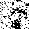
(a)  T=2.30J

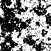
(b)  T=2.35J

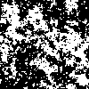
(c)  T=2.45J

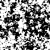
(d)  T=2.55J

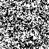
(e)  T=4.50J

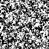
(f)  T=4.52J

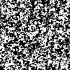
(g)  T=4.55J

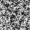
(h)  T=4.60J

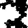
(i)  R=1.00J

(j)  R=1.05J

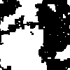
(k)  R=1.10J

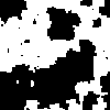
(l)  R=1.15J

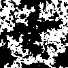
(m)  R=2.25J

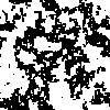
(n)  R=2.26J

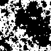
(o)  R=2.27J

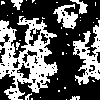
(p)  R=2.28J

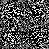
(q)  p=0.31

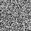
(r)  p=0.50

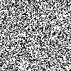
(s)  p=0.59

(t)  p=0.80

Figure 1: Typical critical configurations generated from simulations of clean and random field Ising models and percolation models.

We use numerical simulations to generate typical configurations of metal and insulator domains that can arise from various model Hamiltonians that could potentially be controlling the metal-insulator domain structure. Simulation methods are described briefly in this section and in detail in the SI, and are summarized in Table 1. As VO₂ undergoes a temperature-driven transition from metal to insulator and vice versa, the macroscopic resistivity changes by 4 to 5 orders of magnitude. However, rather than doing so homogeneously, we previously used SNIM to produce spatially resolved images of the metal and insulator domains which revealed that VO₂ thin films transition inhomogeneously, with metal and insulator domains interleaving with each other over a wide range of length scales.Qazilbash et al. (2007); Sohn et al. (2015) We introduce a range of possible Hamiltonians which could be responsible for driving the multiscale textures during the metal-insulator transition in VO₂. Domain configurations from these Hamiltonians will be used to train the DL model to identify the underlying physics driving pattern formation in this material.

Because the experimental probes of interest are directly measuring electronic degrees of freedom, we construct Hamiltonians that are about these electronic degrees of freedom. The intricate patterns of metal and insulator domains happens across multiple length scales from the resolution of the probes all the way out to the field of view ($\approx 20nm-4\mu m$ for SNIM and $\approx 370nm-28\mu m$ for optical microscope data). Therefore, we construct Hamiltonians at the order parameter level. Because the theories are constructed at the order parameter level, they are not microscopic, although they can provide constraints on microscopic models.

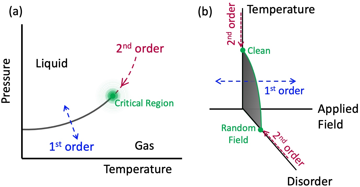
Figure 2: (a) Generic liquid-gas phase diagram above the triple point. For paths along the dotted blue line, the phase transition is first order. However, the transition is second order when approached along the dotted red line. The critical end point (solid green circle) exerts itself over a critical region (open green circles). (b) Phase diagram of the random field Ising model. While the clean or random field Ising model has a second order phase transition as a function of temperature (the red dotted lines), the transition is first order when approached as a function of applied field, crossing through the ordered region (blue dotted line). Critical behavior is observed in the vicinity of the green critical temperature line, whose critical behavior is controlled by the random field fixed point for any finite disorder strength. Because the random field fixed point is a zero temperature fixed point, the critical region is much broader than in the clean case.

First, we consider a clean, interacting Hamiltonian. A reasonable ansatz is that the interaction energy between neighboring domains is lower for like domains than for unlike domains. We model this proclivity toward neighboring like domainsPapanikolaou et al. (2008); Liu et al. (2016a) with a nearest-neighbor Ising Hamiltonian:

$$H=-J\sum_{<i,j>}\sigma_{i}\sigma_{j}-\sum_{i}h\sigma_{i}$$ (1)

where, $\sigma_{i}=\pm 1$ is a two-state local order parameter which in this case tracks metal (e.g., $\sigma=1$) and insulator (e.g., $\sigma=-1$) domains. In an infinite size system, this model undergoes an equilibrium, second order phase transition as a function of temperature at a critical temperature of $T_{c}^{2D}\approx 2.27J$ in two-dimensional systems and $T_{c}^{3D}\approx 4.51J$ in three-dimensional systems. Onsager (1944); Fisher (1974) However, the model also undergoes a first order phase transition as a function of applied field $h$. This first order line terminates in the critical end point mentioned above. The phenomenology of a first order line terminating in a critical end point is why this model is often used in conjunction with the liquid-gas transition. For example, when the liquid-gas transition is approached along the coexistence curve in temperature and pressure, the transition is second order (see the red dotted line in Fig. 2(a)).Kittel and Kroemer (1980) The influence of that critical point is felt throughout a critical region (the light green region in Fig. 2(a)), which includes part of the first order line in the vicinity of the critical end point. Similarly, this model can be used to describe the first order metal-insulator transition in VO₂, with a critical end point whose influence extends along the first order line.Liu et al. (2016a) The physical structure of domains is power law throughout this critical region, when viewed on length scales shorter than the correlation length, which diverges as the critical point is approached. In mapping this order parameter model to the temperature-driven metal-insulator transition in VO₂, we are making the ansatz that a sweep of temperature in the experiment maps to a combination of temperature and field sweep in the model, as in our prior workLiu et al. (2016a) and Ref. Limelette et al. (2003)

Model	Parameters Simulated	Simulation Method
2D Clean Ising (C-2D)	T = $2.25-2.64$	Monte Carlo
3D Clean Ising (C-3D)	T = $4.45-4.65$	Monte Carlo
2D RFIM (RF-2D)	R = $1.00-1.19$	Zero Temperature Field Sweep
3D RFIM (RF-3D)	R = $2.25-2.29$	Zero Temperature Field Sweep
2D Percolation (P-2D)	p = $0.57-0.61$	Biased coin flip
3D Percolation (P-3D)	p = $0.29-0.33$	Biased coin flip
	p = $0.02-0.2$	Biased coin flip
Non-Critical Percolation (P∗)	p = $0.48-0.52$	Biased coin flip
	p = $0.8-0.98$	Biased coin flip

Table 1: Parameters of simulations of the statistical mechanics models. In the first part of the table, parameters are in the critical region. In the second part of the table, parameters are not near criticality.

We simulate configurations near criticality (see Table 1), since that is where this Hamiltonian can cause structure over multiple length scales. We use Monte Carlo simulations to generate typical examples of multiscale morphologies of insulator and metal domains that can arise from the clean Ising Hamiltonians of Eqn. 1. Intricate domain configurations arise near the critical points of this model. Figure 1(a-d) shows some configurations near $T_{c}^{2D}$ on a $100\times 100$ lattice, with periodic boundary conditions. Figure 1(e-h) shows some representative configurations near $T_{c}^{3D}$ on a $100\times 100\times 100$ lattice. Further simulation details are in the SI.

The correlation length of a system diverges at criticality, $\xi\propto 1/|T-T_{c}|^{\nu}$. When viewed on length scales $x<\xi$, the system exhibits critical fluctuations, i.e. fluctuations on all length scales between the correlation length $\xi$ and the short distance cutoff, which for the lattice models we study is the lattice spacing, and in the real physical system it is the size of a unit cell. Close enough to criticality, this length scale will exceed any finite field of view (FOV). Therefore, when observed on a finite FOV (experimentally, or in simulation), there is a finite range of parameters over which the system displays critical pattern formation. For this reason, the entire range of parameters listed in the first part of Table 1 should be viewed as critical for the FOV’s considered in this paper.

In addition to an interaction energy between domains, material disorder also affects the types of shapes that metal and insulator domains take. Because material disorder may make certain regions of the sample more favorable to insulator, and certain others more favorable to metal, we use a random field Ising model (RFIM) to simulate the effects of material disorder on the metal and insulator textures:

$$H=-J\sum_{<ij>}\sigma_{i}\sigma_{j}-\sum_{i}(h_{i}+h)\sigma_{i}$$ (2)

The first term is the clean Ising model of Eqn. 1. In the second term, the uniform field $h$ and the local random fields $h_{i}$ couple directly with the local order parameter. The random fields are chosen from a Gaussian distribution of width $R$ where the probability of $h_{i}$ is $P(h_{i})={\exp(-h_{i}^{2}/(2R^{2}))}/\sqrt{2\pi\sigma^{2}}$. In the physical system, VO₂ changes from insulator to metal as the temperature is changed. Within the model, this physics presents itself as a combination of model temperature and uniform field $h$.Liu et al. (2016a)

The ordered phase corresponds to all metal or all insulator, and the transition is second order when approached as a function of temperature or disorder strength at zero applied field (see the red dotted lines in Fig. 2(b)). When instead the field is swept across the ordered region, the transition is a first order change from metal to insulator (see the blue dotted line in Fig. 2(b)). When temperature and the disorder strength are both nonzero, the behavior of the model in the vicinity of the phase transition is dominated by the random field.Fisher (1986) That is, the random field is relevant but the temperature is irrelevant in the renormalization group sense in a broad range around the solid green line in Fig. 2(b). We therefore model the patterns of metal and insulator domains that are possible with this Hamiltonian by generating domain configurations at zero temperature, while sweeping the uniform field $h$. At zero temperature, this model undergoes an equilibrium phase transition at a random field strength of $R_{c}\approx 2.27J$ in an infinite size three-dimensional system (RF-3D).Middleton and Fisher (2002) In two dimensions (RF-2D), the critical disorder strength is $R_{c}\rightarrow 0$ Perković et al. (1995) in the infinite size limit, although in a finite size system or with finite FOV, $R_{c}(L)>0$. For the FOV we consider, $R_{c}\approx J$ for RF-2D.

When the random field model is near criticality, as the uniform field is swept from low to high or high to low, intricate patterns develop over multiple length scales near the coercive field strength, where the metal/insulator domain fraction changes most rapidly with respect to uniform field $h$. Figures 1(i-l) show representative configurations of RF-2D for a $100\times 100$ lattice. Figures 1(m-p) show representative configurations on the surface of a $100\times 100\times 100$ lattice near the 3D critical disorder strength, $R_{c}^{3D}$.

There is also the possibility that in fact domains are not interacting with each other as in the above Hamiltonians, but rather each domain acts independently. In the corresponding uncorrelated percolation model, a site is labeled “metallic” with a probability $p$; otherwise it is labeled “insulating”. When $p\neq 0.5$, this is like flipping a biased coin where $p$ is the probability of turning up heads. This model also has a second order phase transition as a function of $p$, and displays structure across multiple length scales near its critical point. The critical percolation strength $p_{c}$ is marked by a percolating cluster spanning the entire system, meaning that it touches one side of the system, and also the opposite side. In a two-dimensional system on an infinite square lattice, this threshold occurs at $p_{c}^{2D}\approx 0.59$ and in a three-dimensional system on an infinite cubic lattice it occurs at $p_{c}^{3D}\approx 0.31$. Deng and Blöte (2005) Figure 1(s) shows a percolation configuration of size $100\times 100$ at $p_{c}^{2D}=0.59$. Figure 1(q) shows a percolation configuration $100\times 100\times 100$ at $p_{c}^{3D}=0.31$.

In order to further train the DL model to distinguish configurations that are near criticality (such as those described above) from configurations that are not near criticality, we also generate training images on uncorrelated percolation away from any critical point. In order to avoid the multiscale, fractal textures associated with criticality, in this set of images we use the percolation model in the following ranges: $p=0.02-0.2;~{}0.48-0.52;~{}0.8-0.98$. The first range produces images which are mostly black; the second range produces images which are “white noise” (such as Fig. 1(r)), and the third range produces images which are mostly all white (like those in Fig. 1(t)). Table 1 summarizes the parameter ranges we use for generating simulated data for training and validation from each of the above Hamiltanions.

III Customized Deep Learning Model

Figure 3: Symmetry reduction method, as described in the text.

The parameters from Table 1 are used to generate 8,000 images for each model near its transition, with the exception that percolation away from the 2D and 3D critical percolation strengths accounts for 16,000 images, for a total of 64,000 training images of synthetic data. We describe below the three major components of our Deep Learning model: (A) data preparation via symmetry reduction; (B) a convolutional neural net with multiple layers; and (C) our method for judging the confidence of the classifier.

III.1 Data Preparation: Symmetry Reduction Method

The entire phase space associated with typical configurations generated by the models above satisfies certain symmetries. For example, the clean Ising model (Eqn. 1) satisfies the $Z_{2}$ symmetry ${\sigma_{i}}\rightarrow-{\sigma_{i}}$. Similarly, the RFIM (Eqn. 1) is symmetric under the simultaneous operations ${\sigma_{i}}\rightarrow-{\sigma_{i}}$ with ${h_{i}}\rightarrow-{h_{i}}$. Likewise, the percolation model is symmetric under the simultaneous operations ${\sigma_{i}}\rightarrow-{\sigma_{i}}$ with $p\rightarrow 1-p$. In addition, for the square domain configurations we use as training data, the statistical weight of typical configurations in phase space is symmetric under all of the operations of the dihedral group of the square, $D_{4}$. Such symmetries are often employed in ML via a technique called data augmentation, in which all of the distinct symmetry operations are applied to specific configurations, in order to generate more configurations, and thereby augment the training data. When a neural network is trained under this kind of augmented data set, the resulting trained neural network respects all of the symmetries of the underlying models which produced the training data, rather than suffering from accidental asymmetries which mimic the random nature by which the training data are produced. The number of distinct symmetry operations available in our case is that of $Z_{2}\otimes D_{4}$, or $2\times 8=16$. For the square-shaped images of domain patterns that we generate, using this method of data augmentation would increase the training set by a factor of 16.

Rather than employ data augmentation, we introduce a new method: symmetry reduction. We prepare the data by reducing the symmetry of each configuration as much as possible before feeding it into the neural network. This symmetry reduction is as effective as the data augmentation method, but significantly reduces the time needed to train the neural network. In order for symmetry reduction to be effective, it is essential that all data go through the symmetry reduction before being fed into the CNN (including training, validation, and any subsequent real-world data fed into the classifier).

Let us turn our attention to the $Z_{2}\otimes D_{4}$ symmetry operations in effect. Our models (Eqns. 1 and 2, including the non-interacting percolation limit where $J\rightarrow 0$) map metal and insulator domains to Ising spins $\sigma=+1$ for metal, and $\sigma=-1$ for insulator. There are $2\times 8=16$ symmetry operations that can be applied to these spin configurations while preserving the weights of the typical configurations in phase space. We perform the following symmetry operations to each configuration in order to prepare the data:

1. Ising $Z_{2}$ symmetry ${\sigma_{i}}\rightarrow-{\sigma_{i}}$: If a domain configuration has majority spin down, we flip all spins to make it majority spin up.

2. Rotations by $0,~{}\pi/2,~{}\pi,~{}3\pi/2$: The configuration is rotated such that of the four quadrants, quadrant I has the most spins up.

3. Transpose (reflection about the xy diagonal): If quadrant IV has more spins up than quadrant II, we transpose the configuration to ensure that quadrant II has more spins up than quadrant IV.

All the above operations are performed in the given order and the logic is summarized in Fig. 3.

III.2 Convolutional Neural Net Architecture

Figure 4: Convolutional Neural Network. The input image here is reduced by the symmetry operations given in Fig. 3. The multi-dimensional output 2b is flattened into a one-dimensional array (3a) before it is fed into the fully connected layer. We use the Adam (Adaptive moment estimation) optimization algorithm to train the network. Kingma and Ba (2014) The output label is determined using softmax activation on the output layer.

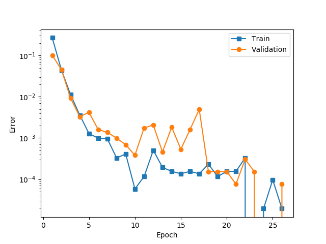
Figure 5: Error in the training and validation set vs. the number of epochs. Epochs correspond to the number of times the training set went through a training process. To prevent overfitting we chose epoch=4 for testing with experimental images. Training/Validation accuracy = 99.64%/99.67%

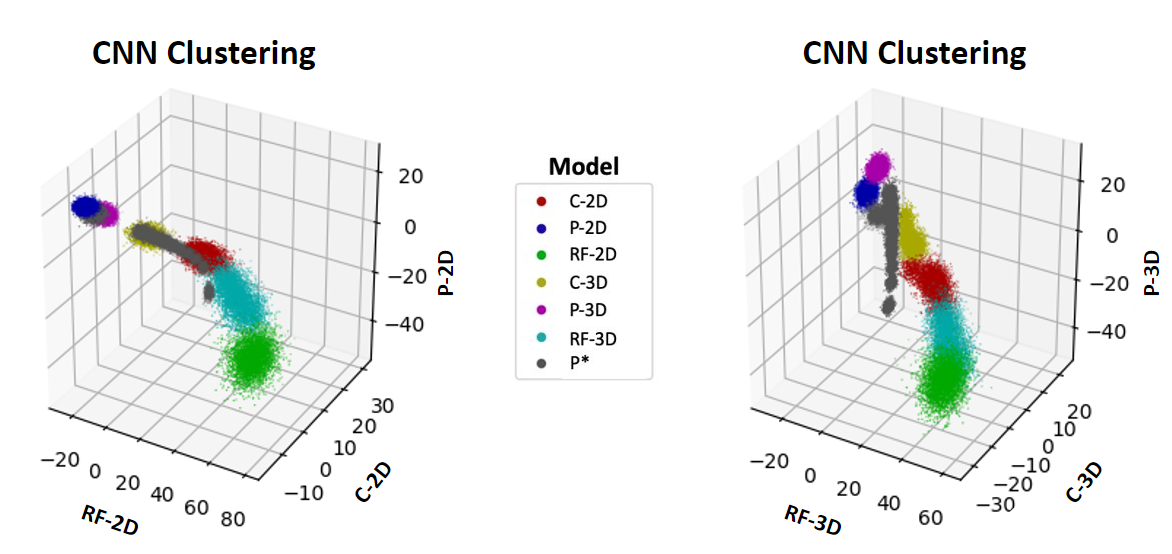
Figure 6: Distribution of values of the output nodes for each class in the last fully connected layer, for all of the training sets. These clusters inhabit a $7$-dimensional “model” space. The two representations in the figure are projections of the same $7$-dimensional information onto two different $3$-dimensional subspaces.

We pass to the neural network single channel binary images (i.e. strictly black and white, the same image space as QR codes) of size $100\times 100$. The architecture of the convolutional neural network (CNN) is as follows (Fig. 4): We use two sets of convolutional layers interleaved with max pooling layers. The first convolutional layer applies a suite of 32 filters of size $5\times 5$ to the image, resulting in an image with 32 channels. (By way of comparison, an RGB image has 3 channels, so that each pixel is described by 3 numbers.) These 32 filters have a total of $32\times 5\times 5$ parameters to be trained. The subsequent max pooling layer groups successive sets of $2\times 2$ pixels, keeping only the largest value in each channel, thus reducing the image size to $50\times 50$. The next convolutional layer applies a suite of 64 filters of size $5\times 5\times 32$ to the 32-channel image which was passed from the previous max pooling layer. These 64 filters have a total of $64\times 5\times 5$ parameters to be trained. This is followed by another max pooling layer, reducing the image size to $25\times 25$ pixels, now with 64 channels.

All of this is followed by a fully connected layer, followed by dropout of 50 % of the connections, followed by a final fully connected layer, resulting in seven-dimensional output for classification (C-2D, C-3D, RF-2D, RF-3D, P-2D, P-3D, and P*). We use a softmax activation in the final output layer, which results in single label classification. If there are $n$ output classes with numbers $v_{i}$, the softmax activation function is defined as:

$$Y_{i}^{softmax}=\exp{(v_{i})}/\sum_{j=1}^{n}\exp{(v_{j})}$$ (3)

where $Y_{i}^{softmax}$ is the output likelihood estimate.

After the symmetry reduction, 80$\%$ of the configurations are used for training; the remaining 20$\%$ are used for validation. The training set is used to train the network whereas the validation set is used to predict the expected error upon generalization beyond the training set. Figure 5 shows how the errors evolve with training epoch. The epoch at which the classification errors in the validation phase deviate from the errors in the training phase roughly marks the onset of overfitting. Figure 5 shows that the classification errors are less than 0.5% at this point.

III.3 Figure of Merit of Classifications

Our goal is to use our ML model developed under supervised learning conditions to distinguish among hypotheses about datasets from real experiments. But before applying our trained ML model to images from experiment, it is important to understand that a trained classifier is only as good as its training set. Thus far, we have generated “simulated data” from various theoretical Hamiltonians, and we have trained an ML algorithm as to which sets of simulated data came from which underlying Hamiltonian. A major challenge in going from simulated data to real-world data is how to control for hypotheses that were not originally envisioned. For example, if an ML classifier has been trained to recognize the difference between cats and dogs, what answer will it give when shown a banana? A simple classifier will give a classification from its training set, but ideally, the answer should not be “cat” or “dog,” but rather, “neither.” Likewise, if our ML classifier is shown experimental data from a system whose underlying Hamiltonian is sufficiently different that none of our Hamiltonians used in the training process are a good description of the physical system, a simple classifier will still return some classification. Therefore, it is necessary to devise a method for flagging potentially dubious classifications. One method is adversarial training, i.e. to train the CNN on images that are not in the set of Hamiltonians comprising the hypothesis. Once again, this is limited by human imagination. For example, how will one know when this process is sufficiently completed, and how can one control for unforeseen image types arising in experiment? It is better to design a neutral method for flagging suspicious classifications, one that is not limited by the adversarial training set.

Therefore, we seek to devise a completely different method for identifying potentially dubious classifications. In order to do this, we turn our attention to the distribution of values observed right after the last fully connected layer in Fig. 4. Fig. 6 shows what the distribution of values looks like at this step, over the entire training set. Since this distribution is well clustered for the seven models of interest, a prediction point lying far from its corresponding cluster should be scrutinized rather than blindly accepted.

For each class, the distribution at the end of the last fully connected layer (see Fig. 6) is generated from the training examples. We form the $7$-dimensional standard deviation vector of these clusters about their centers of mass. We subsequently flag as suspicious any output in this layer that is a distance in this space of more than one standard deviation vector from all points in the cluster. Setting the cutoff at smaller distances rejects too many correct predictions in the validation set. A generalization of this method would be to use any or all of the intermediate layers for detecting such an anomaly in the input data, see Ref. Sivamani et al. (2020).

IV Application to Experimental Images on VO₂

IV.1 Testing the CNN on SNIM images of a thin film of VO₂

We next turn our attention to testing the trained CNN on an experimentally derived dataset for which the Hamiltonian underlying the experimentally observed pattern formation is already known, before applying the CNN to a new experimental dataset for which the answer is not previously known. In this section, we consider experimental data taken via SNIM on a thin film of VO₂. VO₂ undergoes a metal-insulator transition just above room temperature, in which the resistivity changes by over five orders of magnitude.Morin (1959) Rather than transitioning all at once, we previously showed that there is a finite regime of phase coexistence in which the metal and insulator puddles show significant pattern formation.Qazilbash et al. (2007) In fact, the spatial correlations reveal structure on all length scales measured via SNIM, from the pixel size (20nm) all the way out to the field of view (4 $\mu m$).Liu et al. (2016a) The physics driving the pattern formation in this sample is already known via the cluster analysis techniques we recently developed.Phillabaum et al. (2012b); Carlson et al. (2015); Liu et al. (2021) By applying these techniques to analyze the metal and insulator puddles in this thin film of VO₂, we showed that the multiscale domains are of a fractal nature, with quantitative geometric characteristics including avalanche statistics matching those of the RF-2D.Liu et al. (2016a)

Fig. 7 shows the application of the CNN to experimental data on a thin film of VO₂ as it undergoes the metal-insulator transition. The data were obtained using SNIM, and first reported in Ref. Qazilbash et al., 2007. SNIM measurements return an intensity $a$ as a continuous variable at each pixel, resulting in single channel images. These SNIM images are of size 256 px $\times$ 256 px. The SNIM images are converted to black pixels and white pixels by assigning SNIM values of $a<2.5$, which are insulating, to be white, and SNIM values of and $a>2.5$, which are metallic, to be black, as discussed in Ref. Liu et al. (2016a). These thresholded images are shown in the top row of Fig. 7. Ref. Liu et al. (2016a) showed that the geometric characteristics of the pattern formation are insensitive to changes in the threshold $a$ within about 15% of this threshold value.

The CNN takes in the images 100px $\times$ 100px at a time, in each instance returning a classification indicating which Hamiltonian likely produced the pattern formation. In order to make full use of the spatial structure in the image, we use a sliding window of size 100px $\times$ 100px, resulting in $(256-100+1)\times(256-100+1)=157\times 157$ classifications for each image.

In Fig. 8, we show the distribution of values in the last fully connected layer of the CNN, over the set of sliding windows. The small circles correspond to the training set, and are the same as those shown in Fig. 6. The large circles are the result of the CNN applied to the experimentally derived SNIM images. If the large circles lie within one standard deviation of any point in the corresponding training cluster, they are colored black. If the large circles are not within one standard deviation of at least one point within the corresponding validation cluster, they are labeled gray, as described in Sec. III.3.

Fig. 7 shows the final results of the classifier applied to the SNIM data. Below each SNIM image (top row), the bar chart indicates the percentage of sliding windows which give a particular classification. Bright bars and numbers in parentheses correspond to classifications that are within one $7$-dimensional standard deviation of the training sets. The darker part of the bar, and the numbers not in parentheses refer to the the total percentage of sliding windows which give the corresponding classification. Thus the overall result of the ML classifier on an experimentally derived dataset is that it agrees with the classification from cluster techniques, with at least 83$\%$ confidence.

Notice that in Fig. 8, the distribution of values of the output nodes in the last fully connected layer for the CNN applied to the SNIM data is always close to the RF-2D model. Moreover, the entire set of points moves toward the training set distribution and then away from it, as a function of temperature. The temperature of closest approach is T = 342.8K. This same phenomenon is borne out in the bar charts of Fig. 7, where height of the bright green bar also peaks at T = 342.8K. This is highly reminiscent of critical behavior, which grows in strength as the system approaches criticality, and diminishes as the system moves away from criticality. We propose that the distance of the center of mass of the SNIM cluster from the training clusters can be used as a measure of proximity to the critical point. Further study is needed to test this idea.

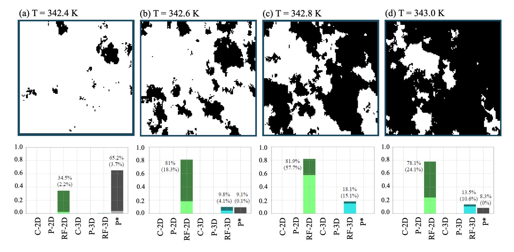
Figure 7: Classification results of our deep learning model applied to SNIM images on a thin film of VO₂ as described in the text. The top row shows the thresholded data as described in the text. The field of view is $4\mu m\times 4\mu m$. White patches are insulating; black patches are metallic. The total percentage of classifications for a particular model are reported in the bar charts of panels (a)-(d). Classification percentages that fall within $1\sigma$ of a cluster in the training set are indicated in parentheses. Classifications that fall more than $1\sigma$ away from the edge of the corresponding cluster in the training set are colored darker in the bar chart.

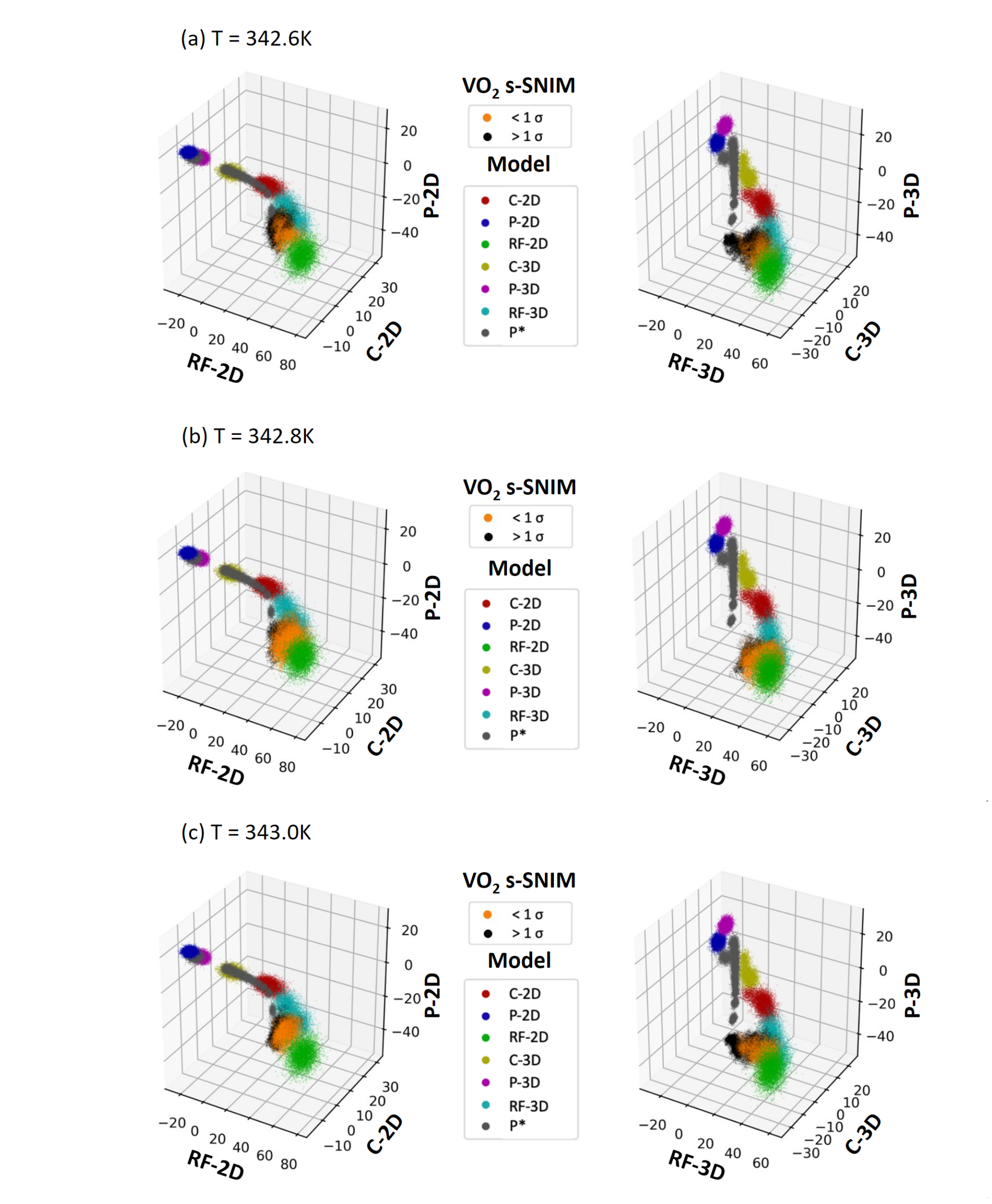
Figure 8: Distribution of values of the output nodes for each class in the last fully connected layer, for the VO₂ SNIM data, superimposed on the distribution for the training sets shown in Fig. 6. Results for the VO₂ data that are within one $7$-dimensional standard deviation of a training set are indicated by orange dots. Results for the VO₂ data that are farther away are indicated by black dots.

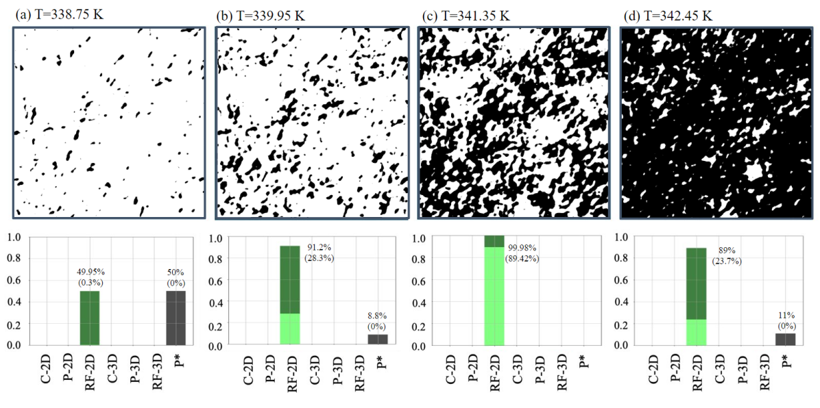
Figure 9: Classification results of our deep learning model applied to new 28$\mu m\times 28\mu m$ optical microscopy images of a VO₂ thin film as described in the text. White patches are insulating; black patches are metallic. The total percentage of classifications for a particular model are reported in the bar charts of panels (a)-(e). Classification percentages that fall within $1\sigma$ of a cluster in the training set are indicated in parentheses. Classifications that fall more than $1\sigma$ away from the edge of the corresponding cluster in the training set are colored darker in the bar chart. All CNN predictions from optical data during a full temperature ramp up are presented in SI Fig. 11.

IV.2 Applying the CNN to New Optical Microscope Images of a VO₂ film

The top panels in Fig. 9 show metal and insulator domains in a thin film of VO₂ made at UCSD, taken using a home-built optical microscopy system capable of remaining in focus while temperature is cycled through the full metal-insulator transition. (See SI and Ref. Alzate Banguero et al. (2022) for full details of the sample preparation and experimental setup.) The optical data are taken at a series of temperatures going through the metal-insulator transition. The physical dimensions of the square image sizes in Fig. 9 are all 28$\mu m\times 28\mu m$, and the pixel size is 50nm. Both the FOV and the pixel size are larger than those of the SNIM images in Fig. 7.

We apply the same sliding window technique as with the SNIM data to analyze pieces of each image, $100$px $\times$ $100$px at a time, in each instance returning a classification indicating which Hamiltonian likely produced the pattern formation. Because the optical images in Fig. 9 are $760\times 760$ pixels, this results in $(760-100+1)\times(760-100+1)=661^{2}$ classifications for each image.

The bottom panels in Fig. 9 show the final results of the CNN classifier applied to the optical microscope data. Below each optical microscope image, the bar chart indicates the percentage of sliding windows which give a particular classification. In this case the images from temperatures T = 339K to T = 343K are each identified as RF-2D with a maximum greater than 89$\%$ confidence. In Figure 10 we show the distribution of values in the last fully connected layer of the CNN, over the set of sliding windows. The small circles correspond to the training set, and are the same as those shown in Fig. 6. We discuss the implications of this identification in Sec. V.

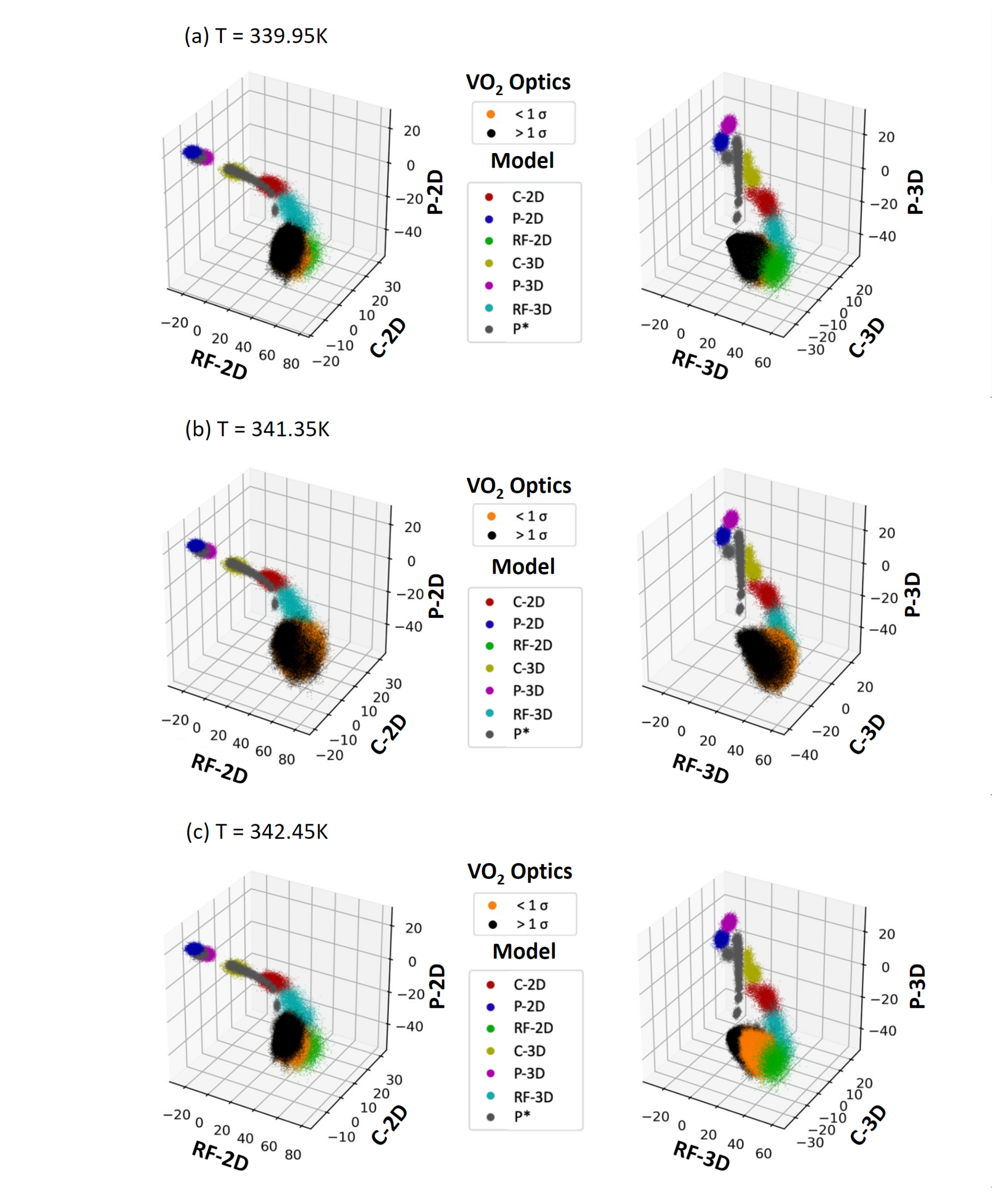
Figure 10: Distribution of relative weights of each class in the last fully connected layer, for the VO₂ optical data (square sample presented in the main text Fig. 9), superimposed on the distribution for the training sets shown in Fig. 6. Results for the VO₂ data that are within one $7$-dimensional standard deviation of a training set are indicated by orange dots. Results for the VO₂ data that are farther away are indicated by black dots.

From a theoretical point of view, we don’t expect every image acquired from the experiments to have significant pattern formation. For example, once the image saturates to metal or insulator, there is no pattern formation left, and consequently there is much less information available in these datasets about the underlying model. Rather, we expect the images to display criticality which reaches peak prominence at a particular temperature. The typical method to discern proximity to criticality is through correlation lengths. The correlation length is expected to blow up as a power law, $\xi\propto 1/|T-T_{c}|^{\nu}$ in the vicinity of the critical temperature. However, the maximum correlation length our CNN can discern is cut off by the maximum FOV that the CNN is fed from the experimental data. Furthermore, the CNN analysis does not return a length scale. Instead, we observe once again the interesting behavior that the proximity of the experimentally derived data’s cluster of output values in the last fully connected layer approaches and then retreats from the cluster of output values in the training sets as a function of temperature, as evidenced by the non-monotonic behavior of the height of the bright green bars with temperature in Fig. 11. This is in line with our previous conjecture that the average distance of the cluster from that of the training set can be used as a measure of proximity to criticality.

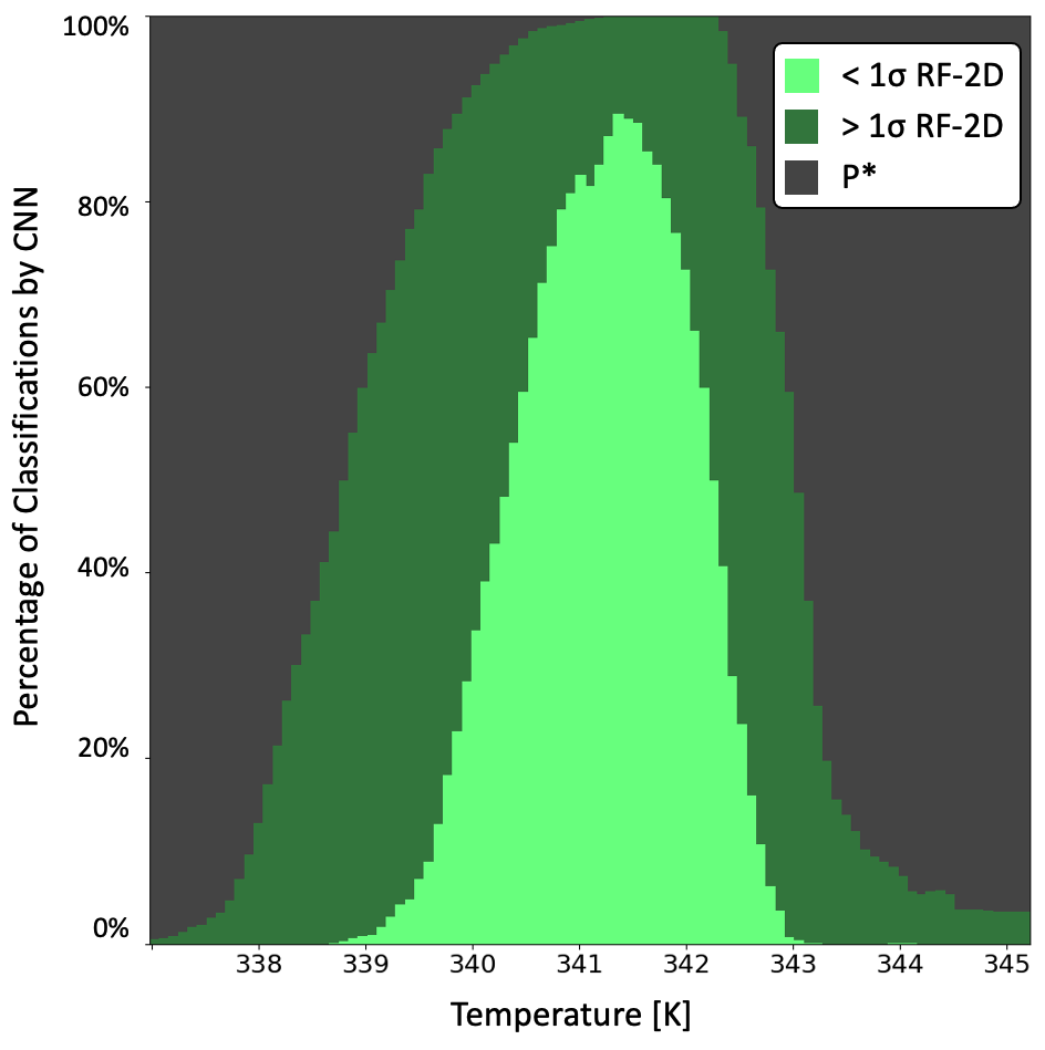
Figure 11: All CNN predictions from optical data during a temperature ramp up of data presented in Fig. 9. Darker colors denote classifications that are more than 1 standard deviation from the identified training set.

V Discussion

For both experimental datasets, whether from SNIM or from optical microscopy, the deep learning CNN determined that the intricate pattern of metal and insulator patches was being set by the physics of the RF-2D. For the SNIM data, this matches our prior identification using cluster methods.Liu et al. (2016a) For the microscope data, it was already known prior to application of the CNN that the physics driving the pattern formation should be arising from a 2D Hamiltonian. This is because the thickness of the film ($\approx 300nm$) is comparable to the lateral resolution of the instrument. Consequently, the spatial correlations being measured are firmly in the two-dimensional limit. However, the fact that the CNN returned a two-dimensional model and not a three-dimensional model gives us further confidence in the CNN method.

The identification of the Hamiltonian as RF-2D means that a combination of material disorder and interactions between spatially proximate regions of the sample drives the pattern formation. The fact that interactions must be present rules out a Preisach modelAlmeida et al. (2001) of independent hysteretic switchers, as we previously argued based on first-order reversal curve measurementsRamírez et al. (2009) and a cluster analysis of the critical exponents during the transition.Liu et al. (2016a) The multiscale nature of the pattern formation is driven by proximity to criticality, which can happen even in a 1st order phase transition, near a critical endpoint.Liu et al. (2016a) Consistent with proximity to criticality, we have previously shown that there is significant slowing down of the relaxation time near the phase transition.Wang et al. (2017); Valle et al. (2019)

Random field critical points exhibit extreme critical slowing down: because the barriers to equilibration grow as a power law as the system nears criticality, the characteristic relaxation time grows exponentially as the system approaches criticality.Fisher (1986) Because of this extreme critical slowing down, the model is notorious for highly nonequilibrium behavior, including hysteresis, glassiness, coarsening, and aging. In addition, the model has an anomalously large region of critical behavior: a system that is 85$\%$ away from the critical point can still display 2 decades of scaling.Perković et al. (1995) This means that it is fairly easy within this model to get into a regime that displays pattern formation across multiple length scales, including fractal textures.

With the model controlling this pattern formation now well established from this study and from our previous workLiu et al. (2016a), we can make the following statements about VO₂: Increasing disorder is expected to broaden hysteresis curves, and also decrease the slope of the hysteresis curve at its inflection point.Sethna et al. (1993a) Indeed, these expectations are borne out in recent ion irradiation studies of resistivity in VO₂.Ramirez et al. (2015) In addition, due to the pronounced memory effects with exponentially long equilibration times, exact identification of material properties can be history-dependent, leading to the appearance of non-repeatability. On the other hand, disorder can ultimately be exploited as another means of controlDagotto (2005); Carlson and Dahmen (2011a).

The ML method is complementary to the aforementioned cluster techniques. Whereas the cluster techniques require at least two decades of scaling in the dataset, we have shown here and in Ref. Burzawa et al. (2019) that an ML classifier can make determinations on datasets with smaller FOV. And while the cluster techniques are designed to extract information from datasets in systems that are in the vicinity of a critical point, we expect that the ML methods developed here can be useful farther away from criticality, because they are able to make determinations on smaller FOV, i.e. they do not require that the system have the long correlation length associated with proximity to criticality.

In the same way that the critical exponents are encoded in the shapes and statistics of the fractal electronic textures that arise near a critical point,Phillabaum et al. (2012b); Carlson et al. (2015); Liu et al. (2016b) our ML study reveals that the universal features of the model itself are encoded in the spatial correlations of the textures, without needing the intermediate step of identifying critical exponents. Criticality presents itself even at the moderate (i.e. not long) length scales our CNN views, which is set by the size of the sliding window we employ on the datasets to be classified.

The method is also potentially extendible to handle non-discrete order parameters, such as continuum models, which present a challenge for cluster methods. For example, it may be possible to use a similar framework to diagnose pattern formation that reveals an underlying XY model or Heisenberg model. In addition, by using regression, we expect to be able to go beyond criticality to begin to determine the values of parameters in the Hamiltonian.

We have developed this ML method first on critical systems, which have no characteristic length scale due to the power law structure, and therefore display spatial structure on every length scale within a correlation length. However, we expect this general scheme to also be broadly applicable to systems that have an emergent length scale, such as frustrated phase separation systems in general, such as block copolymers, the mixed phase of Type I superconductors, reaction-diffusion systems, and convection rolls.Seul and Andelman (1995); Emery and Kivelson (1993)

DagottoDagotto (2005) points out that quenched disorder plays an important role in many strongly correlated materials, and based on this he argues that for such materials, “it is not sufficient to consider phase diagrams involving only temperature and hole-doping x. A disorder strength axis should be incorporated into the phase diagram of these materials as well.” Models incorporating disorder predict that nonequilibrium behavior including glassiness (multiple nearby local energy minima) and hysteresis are prominent features when electronic phase separation occurs in the presence of quenched disorder.Phillabaum et al. (2012b); Carlson et al. (2015); Liu et al. (2016b); Carlson and Dahmen (2011b); Carlson et al. (2006); Loh et al. (2010); Post et al. (2018); Li et al. (2019b); Dahmen and Sethna (1996); Sethna et al. (1993b) The methods we have employed here, which identify the terms in the Hamiltonian, when extended to include a regression analysis to identify the values of the parameters in those terms, have the potential to identify the disorder strength. Mapping out this disorder strength axis in strongly correlated phase diagrams has the potential to help disentangle some of the ambiguities and apparent inconsistencies heretofore reported in the literature of these systems.Timusk and Statt (1999); Armitage et al. (2010); Keimer et al. (2015); Bozovic and Levy (2020)

Future work on this type of classifier will also benefit from: (1) generalizing the CNN to handle input images of any size; (2) developing a learning-based optimization for the rejection classifier; and (3) handling grayscale images without the need to threshold them.

VI Conclusion

In conclusion, we have extended machine learning methods to be able to identify the Hamiltonian driving pattern formation in complex electronic mater. We have shown the accuracy that can be achieved by using a convolutional neural net to classify synthetic data is better than 99%, and about 83–89% accurate on experimental data. We introduce a symmetry reduction method, which significantly lowers the training time over data reduction without reducing accuracy. In addition, we introduce a distribution-based method for quantifying confidence of multilabel classifier predictions, without the problems associated with introducing adversarial training sets. We also propose a new machine learning based criterion for diagnosing proximity to criticality.

We have also demonstrated that this framework can be successfuly applied to real experimental images, by using it to classify the Hamiltonian of SNIM data on a thin film of VO₂, for which the answer was already known from a complementary theoretical method. Having thus vetted our ML model, we applied it to optical microscope data on a different sample of VO₂. In each case, we find that the pattern formation of metal-insulator domains in thin films of VO₂ is driven by proximity to a critical point of the two-dimensional random field Ising model. Further tests of this model include hysteresis protocols in the presence of a series of engineered disorder strengths.

Supplementary Material for

Deep Learning Hamiltonians from Disordered Image Data in Quantum Materials

S1 Experimental Methods

S1.1 Sample Preparation

The VO₂ film measured by optical microscopy was grown by reactive rf sputtering using a stoichiometric V₂O₃ target. The substrate temperature during the growth was 540^oC. The growth was done in 3.4 mTorr 92.3% Ar 7.7% O₂ atmosphere. The rf power was 100 W resulting in  2.5 nm/min growth rate. After the growth, the sample was cooled down at 12^oC/min to room temperature while maintaining the Ar/O₂ atmosphere to preserve proper oxygen stoichiometry in the synthesized film. The film was patterned into 50 $\mu m\times$ 35 $\mu m$ patches by reactive ion etching in Cl₂/Ar atmosphere. Ti/Au electrodes defining 30$\mu m\times$35 $\mu m$ devices were made using standard lithography procedure and e-beam evaporation.

S1.2 Far Field Optical Microscopy

Data for Fig. 9 in the main text are taken using a home-built optical microscopy system capable of remaining in focus while temperature is cycled through the full metal-insulator transition. The 300$nm$ thick film of VO₂, grown at UCSD, was deposited by rf magnetron sputtering on an r-cut sapphire substrate. Gold electrodes separated by 30$\mu$m were deposited on top of the 35$\mu$m etched film Alzate Banguero et al. (2022). As temperature is ramped from 35^oC to 80^o at 0.5^oC/min, the sample shows a clear insulator to metal transition around 68^oC, as evidenced by a change in its resistivity by four orders of magnitude. The images in Figs. 9 and S1 were taken using a home-built optical microscopy system capable of remaining in focus while temperature is cycled through the full metal-insulator transition. Surface reflection images were taken in the visible range with a $\times 150$ magnification dry Olympus objective lens with an optical aperture of 0.9 and a focal point of 1mm. The theoretical lateral resolution is estimated to be $\delta r=1.22\lambda/(2NA)=370nm$ in the visible range using the Rayleigh criterion. Because the equipment (and sample) expand when heated, the sample moves out of the focal plane, and the sample drifts sideways within the field of view upon heating or cooling through the metal-insulator transition. To adress this, at each temperature the objective height is swept through the focal length to create a stack of images. The sharpest (i.e. in focus) image in each stack was selected live by finding the highest image gradient using the Tenengrad function. Liu et al. (2016c) The image recording rate during autofocussing was $\sim$12 images/^oC. The sideways ($xy$) correction was performed post experiment using custom image stabilization software, enabling us to register each pixel within 50nm. Although the pixel size is 50$nm$, we can only resolve structures within the resolution of 370nm. Camera pixel sensitivity was normalized relative to the sapphire substrate in post processing. Alzate Banguero et al. (2022)

When VO₂ is in a uniform insulating or metallic state, the reflectivity is nearly independent of temperature, even though the resistance changes exponentially with temperature in the insulating state. The relative difference between the optical reflictivity in the uniform metal (above T=80^oC) and uniform insulator (below T=50^oC) phases is 20% in the visible range. The raw intensity is recorded in a nearly continuous manner (8-bit grayscale), with fine temperature steps. These fine steps allowed us to use a Gaussian convolution ($\sigma$=2.5) on the raw optical images over 3 frames to reduce high frequency noise. Each pixel’s time trace changes in a sufficiently abrupt manner that it is possible to identify the moment when each spot on the VO₂ film locally undergoes the phase transition. (See Ref. Alzate Banguero et al., 2022 for full details.) This information is then used to produce the black and white (metal and insulator) domain maps shown in Fig. 9.

S1.2.1 Second sample measured by Optics

For consistency we have measured the metal insulator transition in a different VO₂ sample using the optical microscope. The main differences with the data presented in the main text can be listed as such:

• This dataset was taken during a ramp reversal study.Basak et al. (2022) The image recording rate during autofocussing was $\sim$2 images/^oC producing fewer images taken during the insulator to metal transition than the data shown in the main text.

• The gold leads on this sample are separated by only 10 $\mu m$. We apply the same sliding window technique as with the SNIM data to analyze pieces of each image, $100$px $\times$ $100$px at a time, in each instance returning a classification indicating which Hamiltonian likely produced the pattern formation. Because the optical images in Fig. S1 are $500\times 160$ pixels, this results in $(500-100+1)\times(160-100+1)=401\times 61$ classifications for each image.

• The film is 130nm thick.

• The sharpest focus in each stack corresponds to the highest information content, which we identified with a lossless Tiff format using a standard Lempel-Ziv-Welch compression algorithm.Ziv and Lempel (1978); Welch (1984). The gradient method using the Tenengrad function was found to give identical results but is faster computationally.

The ML results presented in Figures S1 and  S2 agree with the results presented in the main part of the paper, Figures 9 and  11.

S2 Clean Ising Models

We simulated the clean Ising model using a mixture of Monte Carlo updates including a parallel checkerboard Metropolis update,Metropolis et al. (1953) as well as the Wolff algorithm.Wolff (1989) The system was thermalized for $100,000$ steps of parallel checkerboard Metropolis interleaved with $10,000$ Wolff updates. After thermalization, spin configurations were saved after $10$ parallel checkerboard Metropolis and $10$ Wolff updates. We simulate systems of size $100\times 100\times 100$, with open boundary conditions (OBC) in the z direction, and periodic boundary conditions (PBC) in the x and y directions. After thermalization, we save spin configurations from the two open surfaces, as well as from 3 paralell 2D slices taken from the interior. All 5 of the 2D spin configurations thus generated are equally spaced. We use a sparse covering in order to minimize correlations between the 2D spin configurations thus obtained. We also save 2D spin configurations from the two orthogonal directions. Since there are periodic boundary conditions in these directions, we can only generate 4 equally spaced configurations perpendicular to the x direction, and 4 perpendicular to the y direction. Thus, a total of $5+4+4=13$ 2D spin configurations are saved from each measurement step of the simulations. This allows us to cover a range of surface effects that can happen in experimental data taken at free surfaces of large bulk samples (i.e. small samples well as large samples viewed on a small window), and save much computational time. If we only use open surfaces of, say, large systems that we window down to a $100\times 100$ FOV, we would need to simulate larger system sizes, typically $400\times 400\times 400$ with OBC, but only save the 6 free surfaces. This method would take $4\times 4\times 4=64$ times longer to simulate, plus we would need to run $13/6\approx 2$ times longer to generate as many configurations. Our method with mixed boundary conditions, and saving some interior and exterior slices, allows us to cover a range of surface effects that can happen at a real surface, where the effective fluctuations can be affected not just by the free surface but also by surface reconstruction effects, but takes $4\times 4\times 4\times 13/6\approx 138$ times less computational time to generate the same number of spin configurations for training. One can see from Fig. 6 that the DL classifier places configurations from both free surfaces and interior slices into the same cluster, rather than producing a distinct cluster for each case.

S3 Simulating multiscale structures

In order to train the DL classifier to recognize multiscale pattern formation in the above models, we simulate them near their transitions and feed these sets of spin configurations into a deep neural network framework that is designed for pattern recognition in images. We generate simulation results from $100\times 100$ (2D) and $100\times 100\times 100$ (3D) lattice size systems.

The parameters from Table 1 are used to generate 8000 images for each model near it transition. The exception is P^∗, which is a set of images not near a transition, for which we generate 16000 images because it covers a larger region of parameter space. Other than P^∗, the models each have a second order phase transition, at which the spin configurations display power law behavior, with structure on all length scales up to the correlation length, which diverges at the critical point. We focus on models near a second order phase transition, because the multiscale behavior inherent to criticality is capable of driving the multiscale pattern formation often seen in spatially resolved experiments on quantum materials.Dagotto and Dagotto (2005); Phillabaum et al. (2012a); Li et al. (2019a); Liu et al. (2016a); Kohsaka et al. (2007); Qazilbash et al. (2007)

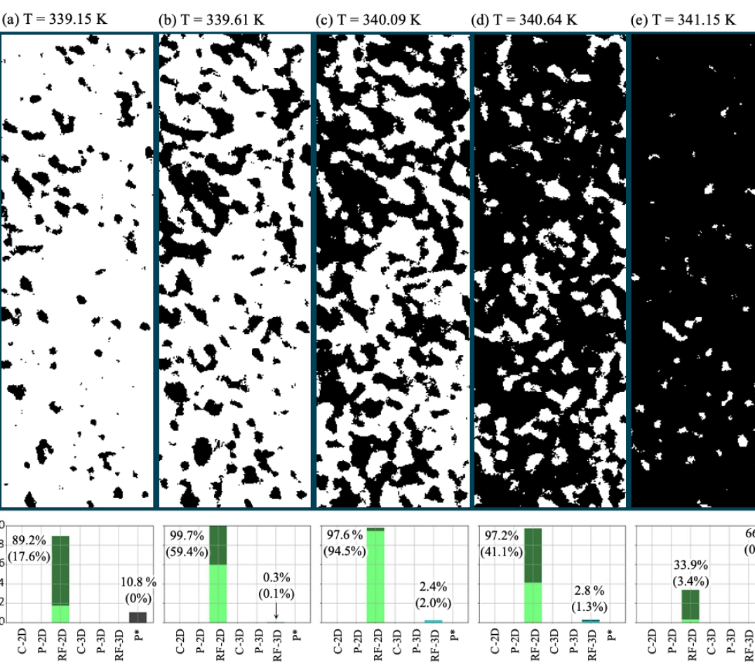
Figure S1: Classification results of our deep learning model applied to optical microscopy images on a second VO₂ film, 7.3$\mu m$ wide by 22.7$\mu m$ long. White patches are insulating; black patches are metallic. The total percentage of classifications for a particular model are reported in the bar charts of panels (a)-(e). Classification percentages that fall within $1\sigma$ of a cluster in the training set are indicated in parentheses. Classifications that fall more than $1\sigma$ away from the edge of the corresponding cluster in the training set are colored darker in the bar chart. All CNN predictions from optical data during a temperature ramp up are presented in SI Fig. S2.

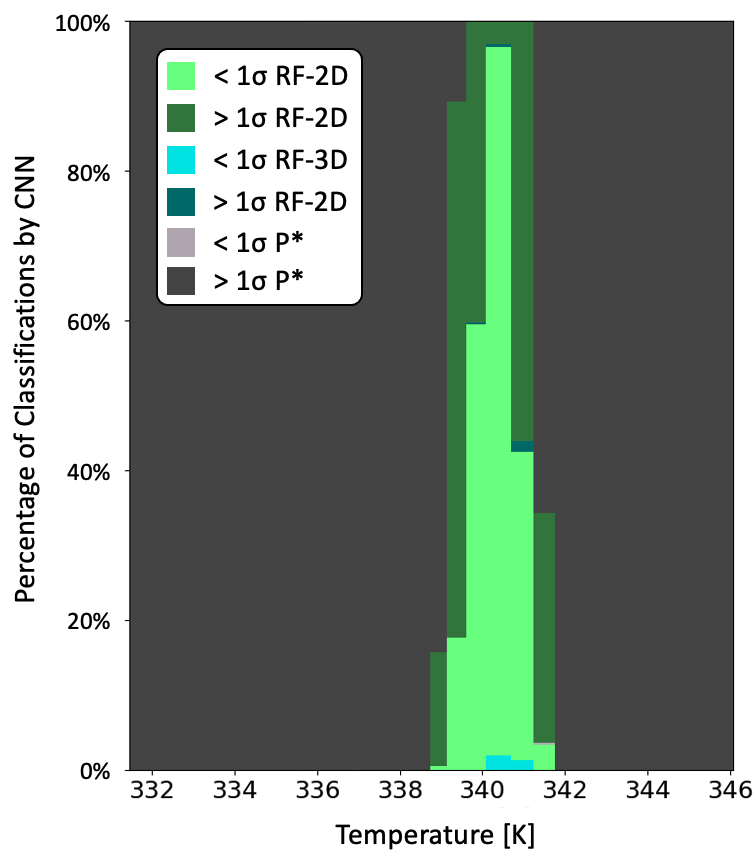
Figure S2: All CNN predictions from optical data during a temperature ramp up of data presented in Fig. S1. Darker colors denote classifications that are more than 1 standard deviation from the identified training set.

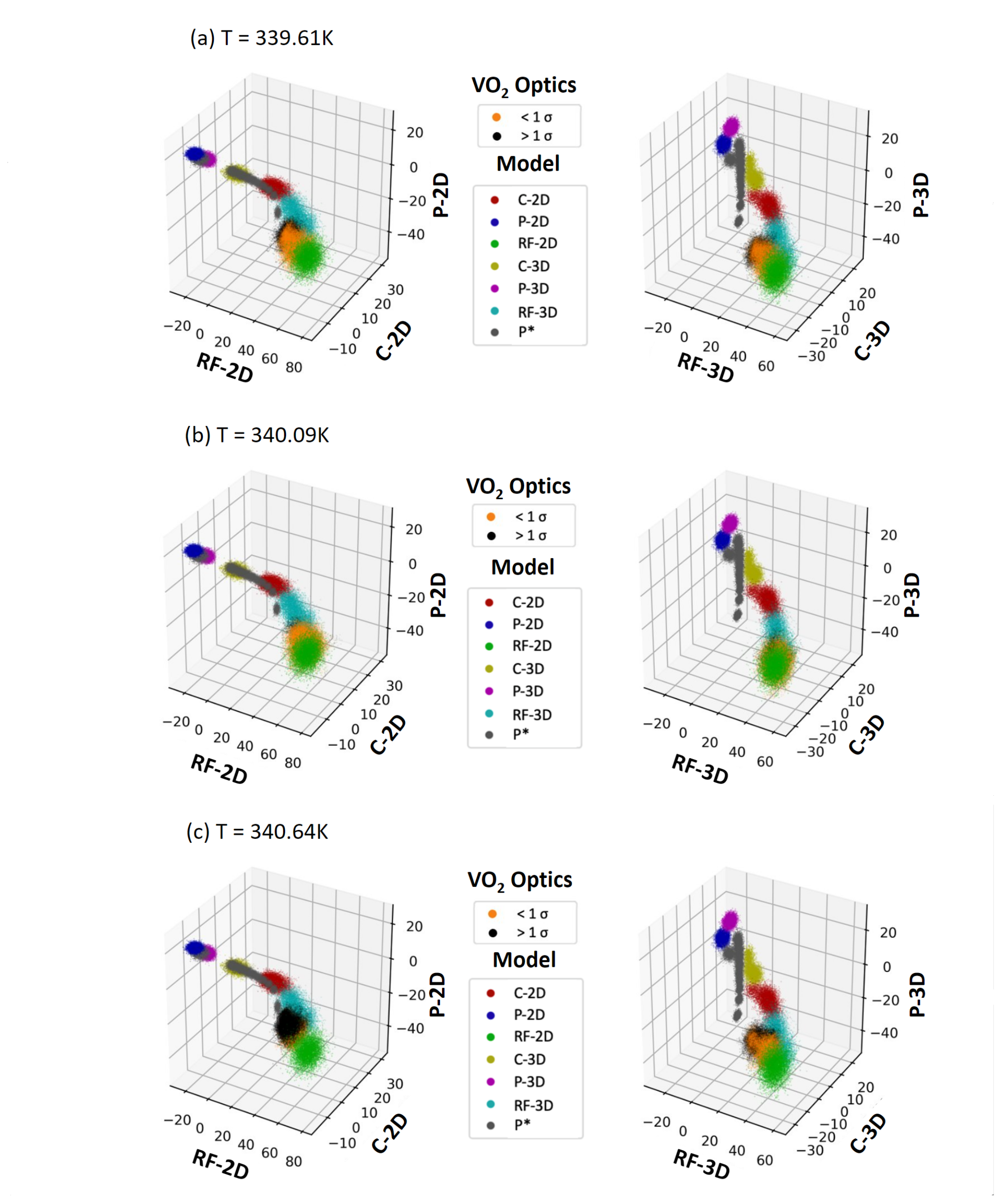
Figure S3: Distribution of relative weights of each class in the last fully connected layer, for the VO₂ optical data (rectangular second sample presented in the supplementary text Sec. S1.2.1 and Fig. S1), superimposed on the distribution for the training sets shown in Fig. 6. Results for the VO₂ data that are within one $7$-dimensional standard deviation of a training set are indicated by orange dots. Results for the VO₂ data that are farther away are indicated by black dots.