PI is back! Switching Acquisition Functions
in Bayesian Optimization

Abstract

Bayesian Optimization (BO) is a powerful, sample-efficient technique to optimize expensive-to-evaluate functions. Each of the BO components, such as the surrogate model, the acquisition function (AF), or the initial design, is subject to a wide range of design choices. Selecting the right components for a given optimization task is a challenging task, which can have significant impact on the quality of the obtained results.
In this work, we initiate the analysis of which AF to favor for which optimization scenarios. To this end, we benchmark SMAC3 using Expected Improvement (EI) and Probability of Improvement (PI) as acquisition functions on the 24 BBOB functions of the COCO environment. We compare their results with those of schedules switching between AFs. One schedule aims to use EI’s explorative behavior in the early optimization steps, and then switches to PI for a better exploitation in the final steps. We also compare this to a random schedule and round-robin selection of EI and PI.
We observe that dynamic schedules oftentimes outperform any single static one. Our results suggest that a schedule that allocates the first $25\text{\,}\mathrm{\char 37\relax}$ of the optimization budget to EI and the last $75\text{\,}\mathrm{\char 37\relax}$ to PI is a reliable default. However, we also observe considerable performance differences for the 24 functions, suggesting that a per-instance allocation, possibly learned on the fly, could offer significant improvement over the state-of-the-art BO designs.

1 Introduction

Bayesian Optimization (BO) [Mockus, 2012] is a technique to find the global optimum of black-box problems when each evaluation of the objective function is expensive or otherwise resource-intensive, e.g., problems requiring elaborated physical experiments or computationally-heavy simulations. BO is widely known as one of the most efficient black-box approaches in terms of number of function evaluations required, hence a promising tool for the optimization of low-budget problems.

BO is defined as a modular framework which consists of (i) defining an initial set of points where the true (unknown, expensive) objective function is evaluated, (ii) approximating the objective function based on the initial design by placing a prior probability distribution on it (i.e., building a surrogate model), (iii) selecting where to sample next by optimizing an acquisition function (also known as infill criterion) that takes care of the trade-off between exploration and exploitation, (iv) evaluating new samples on the true objective function, and finally (v) computing the posterior probability distribution on the true objective function based on new knowledge, hence updating the surrogate model. Steps (iii) to (v) are repeated iteratively until the evaluation budget is exhausted.

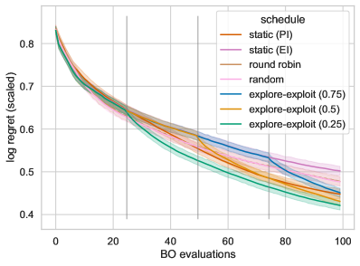
Figure 1: Switching AFs is beneficial. Scaled log-regret averaged over all $24$ BBOB functions for $5$ dimensions with the $95\text{\,}\mathrm{\char 37\relax}$ confidence interval for the schedules from Figure 2.

Name	Schedule
static (EI)
static (PI)
random
round robin
explore-exploit ($0.25$)
explore-exploit ($0.5$)
explore-exploit ($0.75$)

Figure 2: Schedule portfolio of PI, EI and their combinations.

Each component of the sequential BO pipeline is subject to a wide range of design choices, which in turn affects the overall performance of the BO procedure [Lindauer et al., 2019; Cowen-Rivers et al., 2021; Bossek et al., 2020]. For example, each acquisition function (AF) exhibits different behavior, with some being more explorative and others more exploitative. To date, design choices have been predominantly static during BO execution. However, other areas of optimization indicate that dynamic choices can lead to performance gains Karafotias et al. [2015]; Doerr and Doerr [2020]; Adriaensen et al. [2022].

In this work, we investigate whether the same applies to BO. Specifically, we propose a dynamic schedule that switches between two AFs, namely Probability of Improvement (PI) and Expected Improvement (EI) Forrester et al. [2008], during the BO procedure. This simple approach is already quite effective and outperforms any single static schedule on most problems. We assess our method on the BBOB test suite from the COCO library [Hansen et al., 2021], which is a standard benchmark in black-box optimization. We purposely opt for such a benchmark in order to shift focus from a purely performance-oriented view towards understanding the problem characteristics that favor one or the other AF, which is a stark difference between this paper and previous works on dynamic AF selection. We thus observe that the choice of schedule is largely problem-dependent and that further investigation in this direction is of utmost importance to fully understand and exploit the untapped potential of adaptive AF selection.

Background Since our approach is focused on PI and EI, we briefly recall their formulations:

$$\text{PI}(x)=\Phi\left(\frac{\Delta(x)}{\sigma(x)}\right)\quad\text{and}\quad\text{EI}(x)=\begin{cases}\Delta(x)\ \Phi\left(\frac{\Delta(x)}{\sigma(x)}\right)+\sigma(x)\ \phi\left(\frac{\Delta(x)}{\sigma(x)}\right)&\mbox{if }\sigma(x)>0\\ 0&\mbox{if }\sigma(x)=0\end{cases}$$

with $\Delta(x)=y_{\text{min}}-\mu(x)$, where $y_{\text{min}}$ is the best observed value so far, and the mean $\mu(x)$ and the variance $\sigma^{2}(x)$ are queried from the posterior of the surrogate model – in our work a Gaussian Process (GP). $\Phi$ and $\phi$ are the Gaussian cumulative distribution function and probability density function, respectively. By definition, in a minimization problem, the maximization of PI drives the selection of new candidates for evaluation towards areas of the domain where the mean value of the GP model is low. On the contrary, EI balances exploitation (thanks to the first summation term) and exploration (second summation term) by alternating sampling in promising areas of the domain according to the mean value and unexplored ones, where the variance of the GP model is high. Comparing both, EI is more explorative and PI more exploitative, see Appendix A for an example.

Related Work We first present existing work on AFs and focus on different approaches considering AFs. Important findings are reported when the main target is to improve and develop better AFs, from enhancing EI [Qin et al., 2017; Balandat et al., 2020] to meta-learning neural AFs [Volpp et al., 2020]. A different line of work is concerned with combining different AFs, e.g. by building a portfolio of AFs (EI, P̧I, Upper Confidence Bound (UCB) with different hyperparameter settings) and then using an online multi-armed bandit strategy to assign probabilities of which AF to use at which step, called GP-Hedge [Hoffman et al., 2011]. Their work indicates that the performance of GP-Hedge highly varies with the number of arms and their respective hyperparameter settings. Similarly to GP-Hedge, Kandasamy et al. [2020] update weights of their portfolio (UCB, EI, Thompson Sampling (TS) [Thompson, 1933], Top-Two Expected Improvement (TTEI) [Qin et al., 2017]) in an online manner. They do not include PI as they observe it exhibits inferior performance compared to other single static AFs. In addition, robust versions of EI, PI and UCB can be combined to a multi-objective AF combining the strengths of the individual ones [Cowen-Rivers et al., 2021]. In contrast to the existing literature, we here take a step back and ask ourselves what we could achieve by employing a simplistic approach of switching between AFs through a dynamic schedule.

It has also been shown in other optimization-related areas that dynamic choices are beneficial in terms of performance, e.g. in evolutionary computation Karafotias et al. [2015]; Doerr and Doerr [2020], planning [Speck et al., 2021] and deep learning [Adriaensen et al., 2022]. Recently, the introduction of Dynamic Algorithm Configuration (DAC) [Biedenkapp et al., 2020] underlines the potential of training dynamic schedules (as opposed to selecting algorithm components on the fly, as is usually done in evolutionary computation Hansen et al. [2003]).

2 Proposed Method

To evaluate the potential of dynamic AF schedules, we consider several different variants, summarized in Figure 2. As baselines, we use static schedules, namely EI and PI. Two types of dynamic schedules are considered: alternating and switching. The former go back and forth between EI and PI, whereas the latter make a single switch from EI to PI after a pre-defined percentage of the budget has been spent. We introduce two alternating schedules as baselines for a dynamic approach: random and round robin. For the random schedule the AF is chosen uniformly at random before a new solution is sampled, while round robin simply alternates the AFs for each sample. Finally, three different switching schedules are considered, making a switch after $25\text{\,}\mathrm{\char 37\relax}$, $50\text{\,}\mathrm{\char 37\relax}$ and $75\text{\,}\mathrm{\char 37\relax}$ of the budget remaining after the initial design (i.e., surrogate-based function evaluations), respectively. This makes it possible to investigate whether the conceptual idea of switching is beneficial and additionally gives insight into the effects of switching at different stages of the optimization process.

3 Experiments

We evaluate our schedules on the $24$ single-objective noiseless BBOB functions of the COCO benchmark [Hansen et al., 2021] in dimensions $5$ with $60$ seeds (i.e., we perform $60$ independent runs on each problem and for each AF schedule). We optimize our functions with an initial design (or: Design of Experiment (DoE)) of $3d=15$ data points and BO length of $20d=100$ function evaluations. Per seed, the initial design is the same for every schedule. To create the dynamic BO, SMAC3 [Lindauer et al., 2022] is adapted accordingly and we use a GP as surrogate model. All experiments were conducted on a Slurm CPU cluster with $1592$ CPUs available across nodes. For visualization, we consider the log-regret of the incumbent (best evaluated search point) and only visualize the evaluations proposed by BO, omitting the initial design. In the violin plots the log-regrets of the final incumbents of all $60$ seeds are normalized to $[0,1]$ per BBOB function. In the convergence plots the log-regret of the incumbents of all $60$ seeds over all evaluations are normalized to $[0,1]$ per BBOB function and the means with the $95\text{\,}\mathrm{\char 37\relax}$ confidence intervals are shown. The plots for each function can be found in Appendix B. The code can be found here: https://github.com/automl/pi_is_back.

Observations

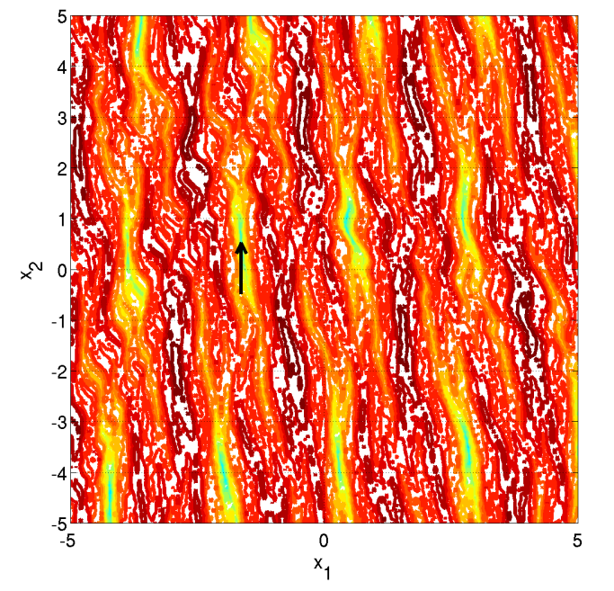
(a) Landscape of Weierstrass (F16) [Hansen et al., 2021]

(b) Log-Regret (Scaled) per Step

Figure 3: BBOB Function 16: Highly rugged and moderately repetitive landscape with many local optima. Dynamic schedules outperform static ones and we can clearly observe the boost gained after switching from EI to PI.

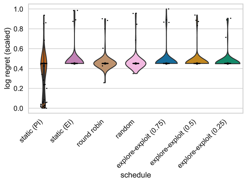
(a) Final Log Regret (Scaled)

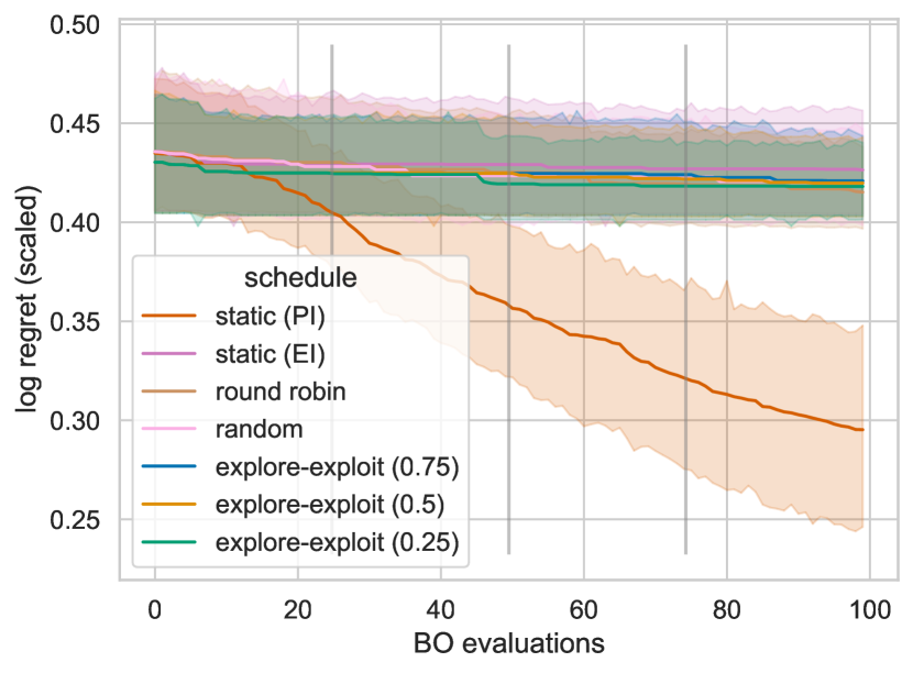
(b) Log-Regret (Scaled) per Step

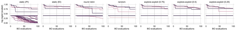
(c) Log-Regret (Scaled) per Step and Seed

Figure 23: BBOB Function 19

A first observation is that switching from EI to PI is in general beneficial when the function landscape has an adequate global structure (F1-F19). Here, the only exceptions are F5 and F19. F5 is a purely linear function, where EI performs best as it explores fast in the beginning and exploits sufficiently fast later on because of the simplicity of the landscape. For F19, we hypothesize that only PI is able to exploit a lucky initial design landing close to optima as indicated by the individual runs in Figure 23(c).

In addition, we can see that PI works well for uni-modal and quite smooth functions (F1-F14), and even better when used after the switch. This observation is in line with PI’s exploitative behavior. In these cases exploiting does not miss any other optima further away in the landscape.

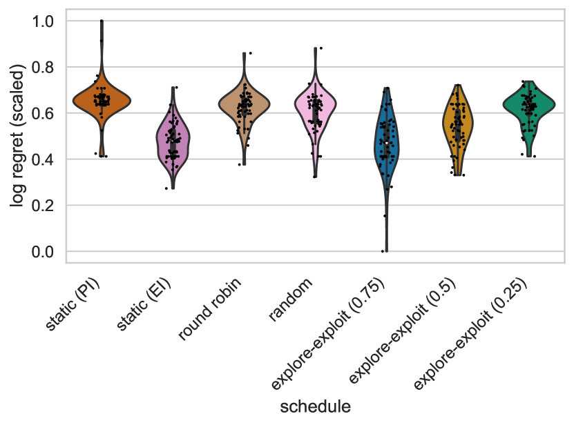
(a) Final Log Regret (Scaled)

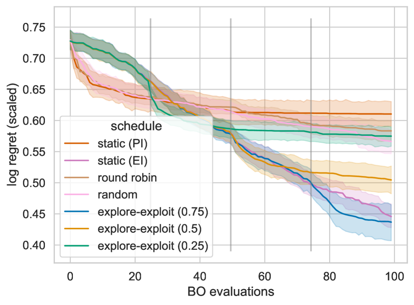
(b) Log-Regret (Scaled) per Step

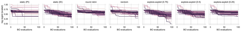
(c) Log-Regret (Scaled) per Step and Seed

Figure 11: BBOB Function 7

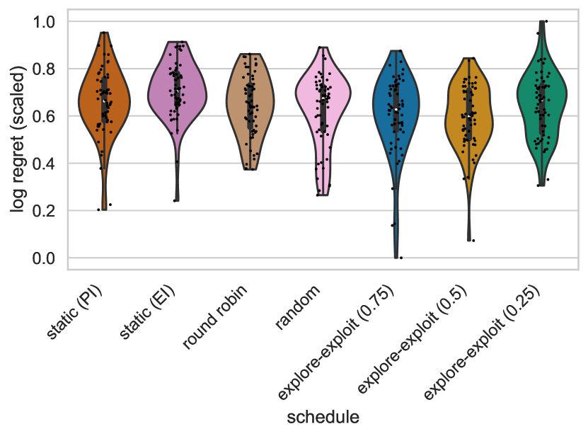
(a) Final Log Regret (Scaled)

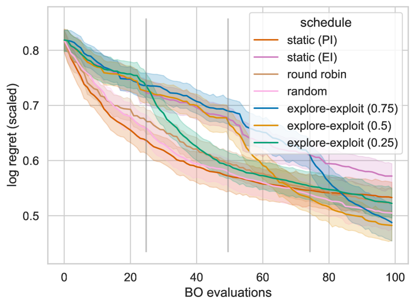
(b) Log-Regret (Scaled) per Step

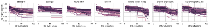
(c) Log-Regret (Scaled) per Step and Seed

Figure 27: BBOB Function 23

In contrast, PI is in general worse than EI and also not beneficial after the switch for multi-modal functions with weak global structure (F20-F24). Again, this is in line with our intuition because for these functions we have many important basins of attraction that have to be discovered before starting exploitation. The only exception is F23 (Figure 27), a rugged function with a high number of global optima, where the probability of starting in a basin of attraction is high and thus exploitation is a viable strategy. Also, the flatter the landscape the worse PI performs which can be also seen in F7 (slope with step, Figure 11).

Besides the static and the switching schedules, round robin switches from EI to PI and vice versa for each new function evaluation. The round robin schedule creates a step-wise progress, but is never the best strategy. Apparently, less frequent switching is preferable in order to take advantage of the strengths of each AF. On average, the random schedule performs similarly to round robin, but with a smoother progression. Most likely, the random schedule still switches too frequently for the AFs to work effectively.

On F16 we observe that a late switch from EI to PI performs best, see Figure 3(b). We can also nicely spot the general boosts after switching after $25\text{\,}\mathrm{\char 37\relax}$, $50\text{\,}\mathrm{\char 37\relax}$ and $75\text{\,}\mathrm{\char 37\relax}$. F16 has a highly rugged and moderately repetitive landscape with many local optima with evident quality difference. Therefore, PI can be trapped in a bad local optimum if applied too early.

Key Insights To summarize our observations, the general optimal choice of static or dynamic AF schedules depends on the problem at hand. Plus, switching from EI to PI after a certain percentage of the budget of total number of function evaluations is beneficial and can boost performance. However, the optimal switching point depends on the problem. On average, switching after $25\text{\,}\mathrm{\char 37\relax}$ seems to be best and is a viable schedule if the problem’s properties are unknown.

4 Conclusions and Future Work

In this work we acknowledge the modular structure of Bayesian Optimization (BO) and explore different acquisition function schedules composed of Expected Improvement (EI) and Probability of Improvement (PI), with the premise that a dynamic choice would boost BO performance. We evaluate our approach on a standard benchmark for black-box optimization, and observe that dynamic acquisition function (AF) schedules often outperform single static ones, although their performance depends on the problem at hand. As a general recommendation, if the properties of the problem to optimize are unknown, switching from EI to PI after $25\text{\,}\mathrm{\char 37\relax}$ of the budget of surrogate-based evaluations should be favored. We also highlight some key insights into the interplay of the nature of the problem and the performance of the proposed approach.

These preliminary findings suggest the potential of the dynamic choices in a BO pipeline merit further investigation. As future steps in this direction, finding the most appropriate schedule of different AFs is an open problem we could tackle with meta-learning. One way would be to train models recommending which AF to use at which step based on problem representation, i.e., typically Exploratory Landscape Analysis (ELA) features [Mersmann et al., 2011]. In addition, finding meaningful state features could enable an online selection of the AF via heuristics or Reinforcement Learning [Adriaensen et al., 2022]. To this end, besides elapsed time and progress being default choices as state features, we could incorporate properties of the surrogate model to serve as a guide to select the AF. Furthermore, including more AFs and their hyperparameters in the portfolio, as well as dynamically changing other components of BO, like the surrogate model, the GP kernel, or the optimizer of the AF, might increase overall performance and sample-efficiency of BO.

Acknowledgments

Our work has been financially supported by the the ANR T-ERC project VARIATION (ANR-22-ERCS-0003-01), by the CNRS INS2I project RandSearch, and by the PRIME programme of the German Academic Exchange Service (DAAD) with funds from the German Federal Ministry of Education and Research (BMBF), and by RFBR and CNRS, project number 20-51-15009. Carolin Benjamins and Marius Lindauer acknowledge funding by the German Research Foundation (DFG) under LI 2801/4-1.

Appendix A Exploration vs. Exploitation

We choose EI and PI to build our AF schedules because of their different search behavior. In Figure 4 we exemplarily show EI’s explorative character and PI’s exploitative character. Both behaviors can be beneficial depending on the problem to optimize.

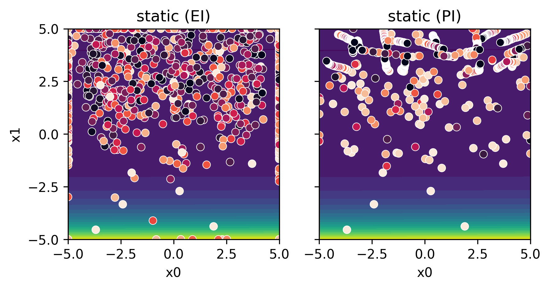
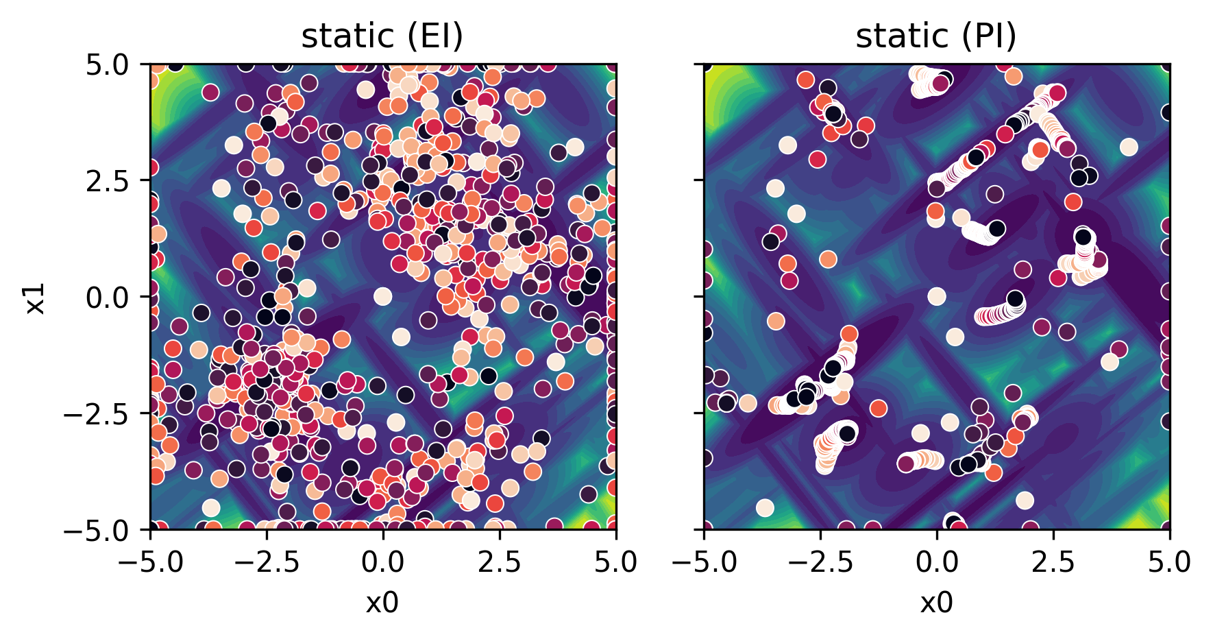
Figure 4: EI vs. PI on BBOB function 12 (upper) and 21 (lower). The dots indicate the visited configuration at a certain step. We visualize all $20$ seeds with an initial design size of $10$ (not plotted) and $40$ BO evaluations.

Appendix B Additional Results

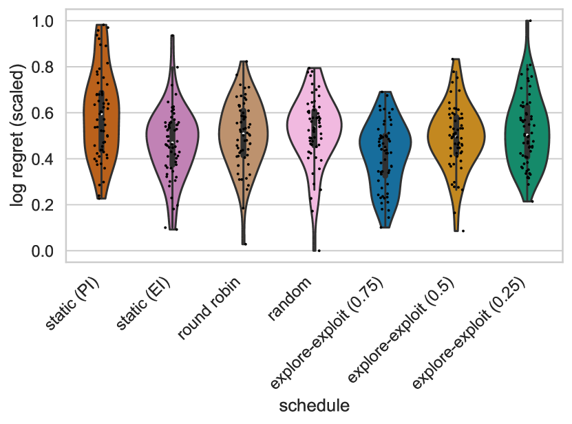
(a) Final Log Regret (Scaled)

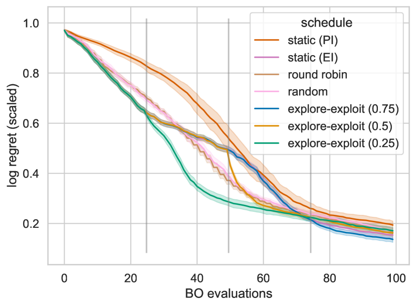
(b) Log-Regret (Scaled) per Step

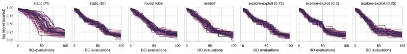
(c) Log-Regret (Scaled) per Step and Seed

Figure 5: BBOB Function 1

(a) Final Log Regret (Scaled)

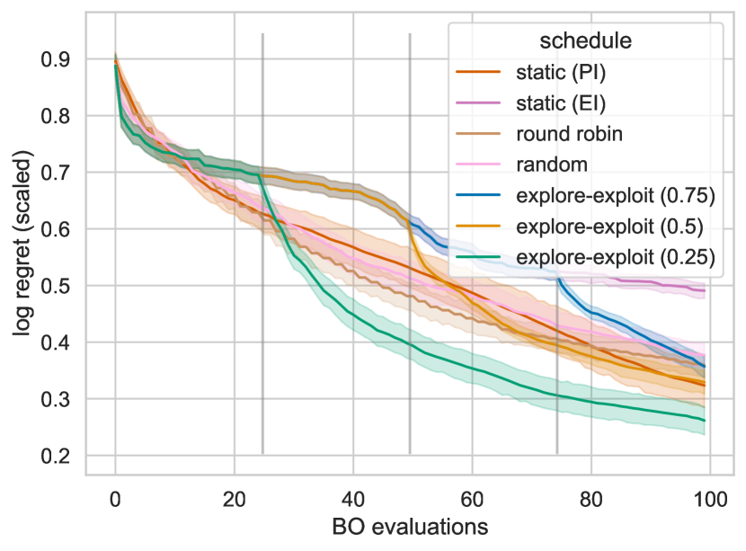
(b) Log-Regret (Scaled) per Step

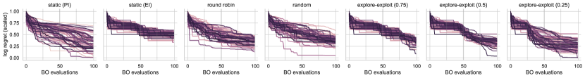
(c) Log-Regret (Scaled) per Step and Seed

Figure 6: BBOB Function 2

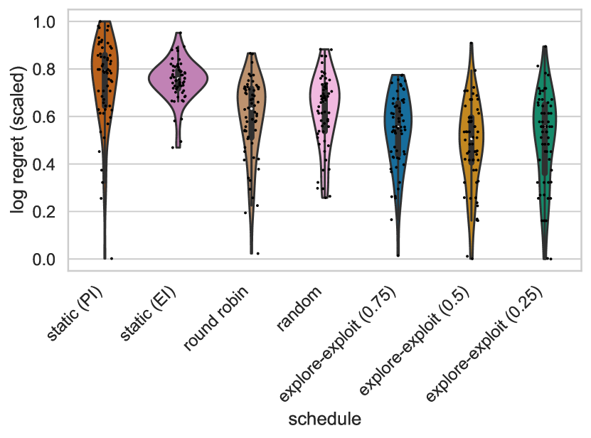
(a) Final Log Regret (Scaled)

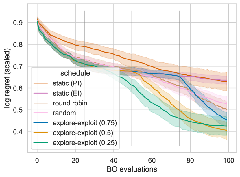
(b) Log-Regret (Scaled) per Step

(c) Log-Regret (Scaled) per Step and Seed

Figure 7: BBOB Function 3

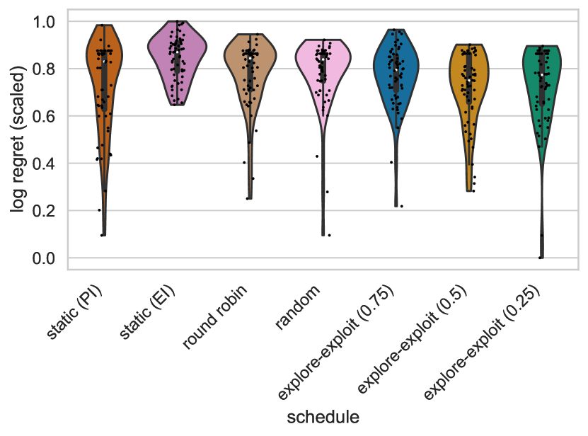
(a) Final Log Regret (Scaled)

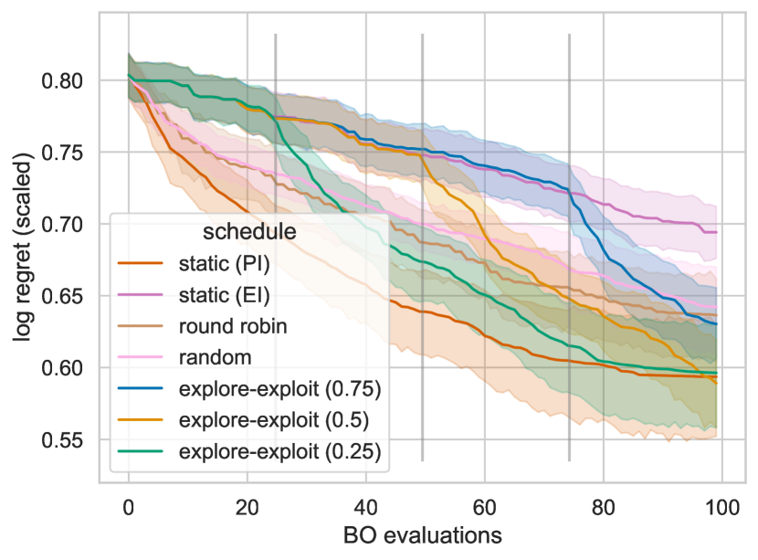
(b) Log-Regret (Scaled) per Step

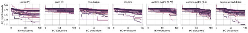
(c) Log-Regret (Scaled) per Step and Seed

Figure 8: BBOB Function 4

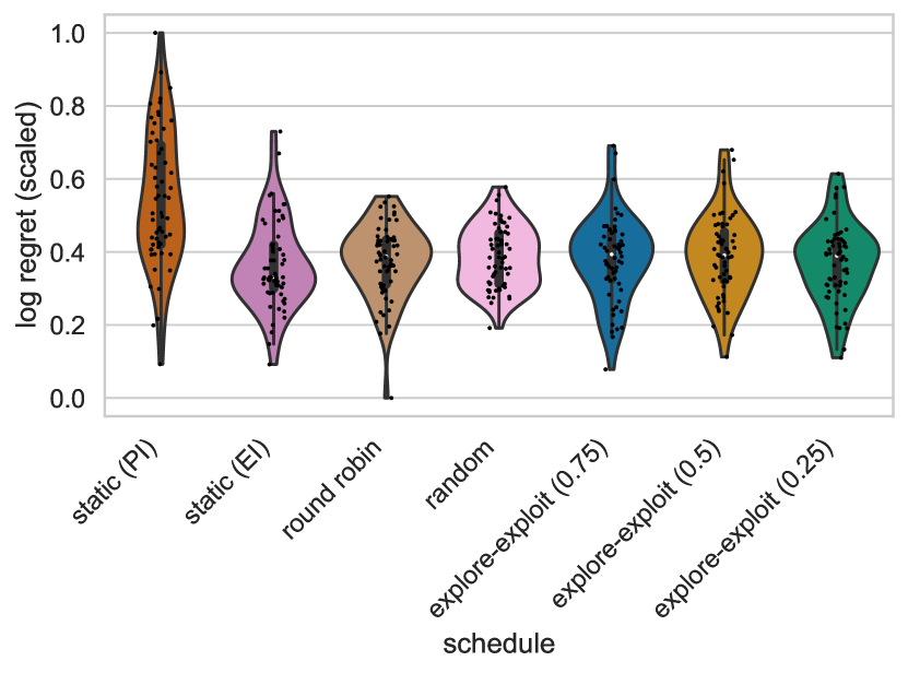
(a) Final Log Regret (Scaled)

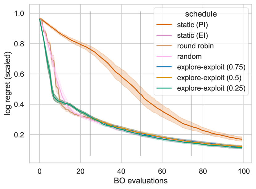
(b) Log-Regret (Scaled) per Step

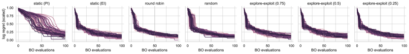
(c) Log-Regret (Scaled) per Step and Seed

Figure 9: BBOB Function 5

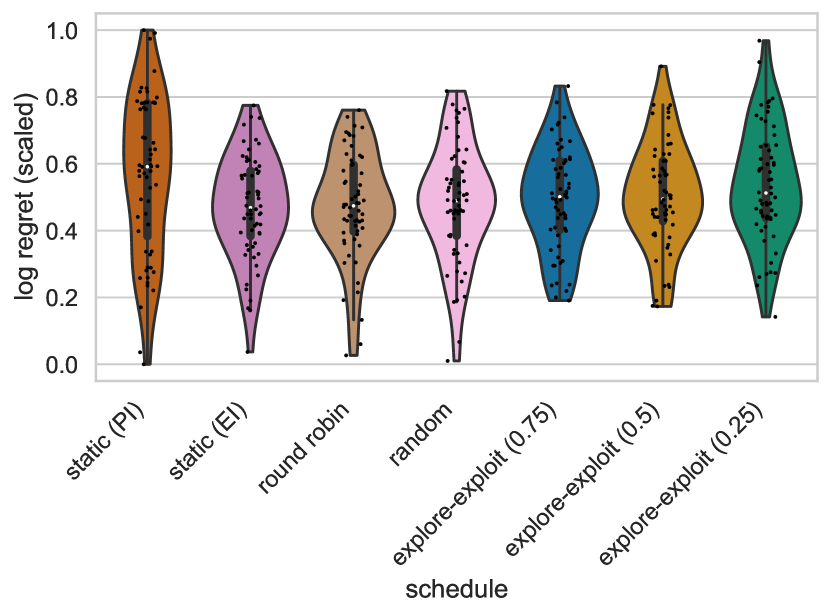
(a) Final Log Regret (Scaled)

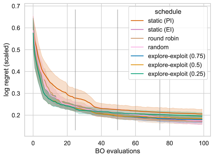
(b) Log-Regret (Scaled) per Step

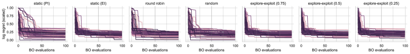
(c) Log-Regret (Scaled) per Step and Seed

Figure 10: BBOB Function 6

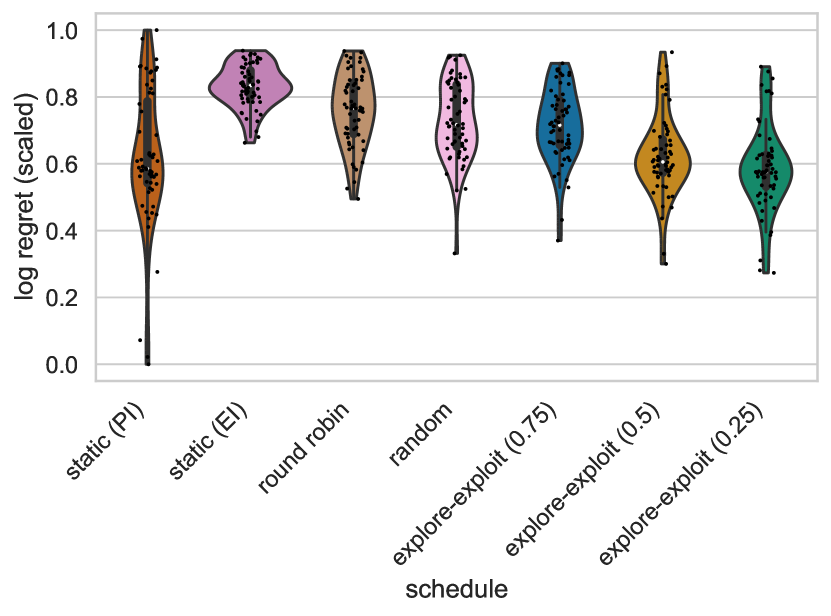
(a) Final Log Regret (Scaled)

(b) Log-Regret (Scaled) per Step

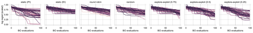
(c) Log-Regret (Scaled) per Step and Seed

Figure 12: BBOB Function 8

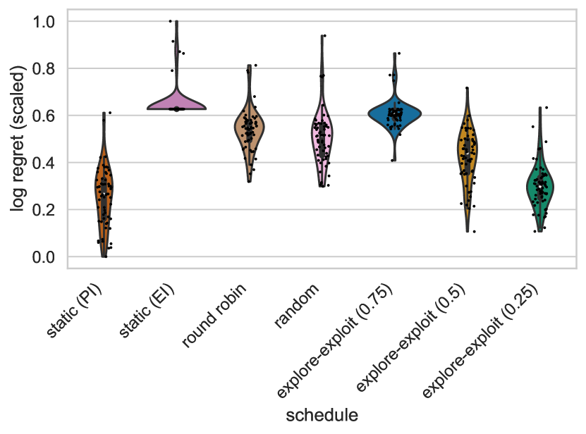
(a) Final Log Regret (Scaled)

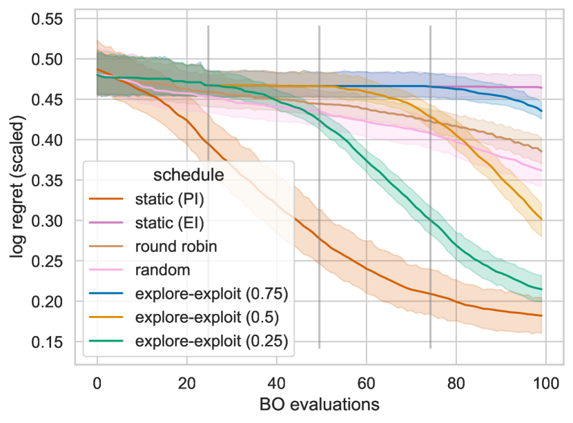
(b) Log-Regret (Scaled) per Step

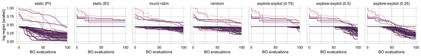
(c) Log-Regret (Scaled) per Step and Seed

Figure 13: BBOB Function 9

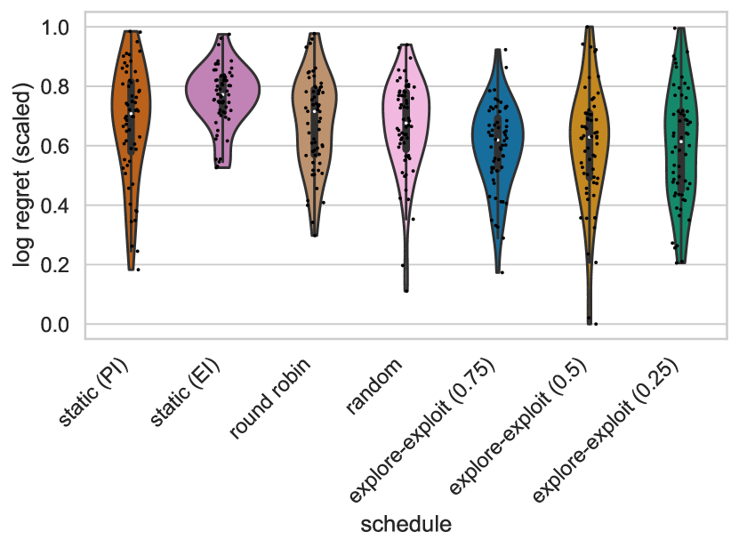
(a) Final Log Regret (Scaled)

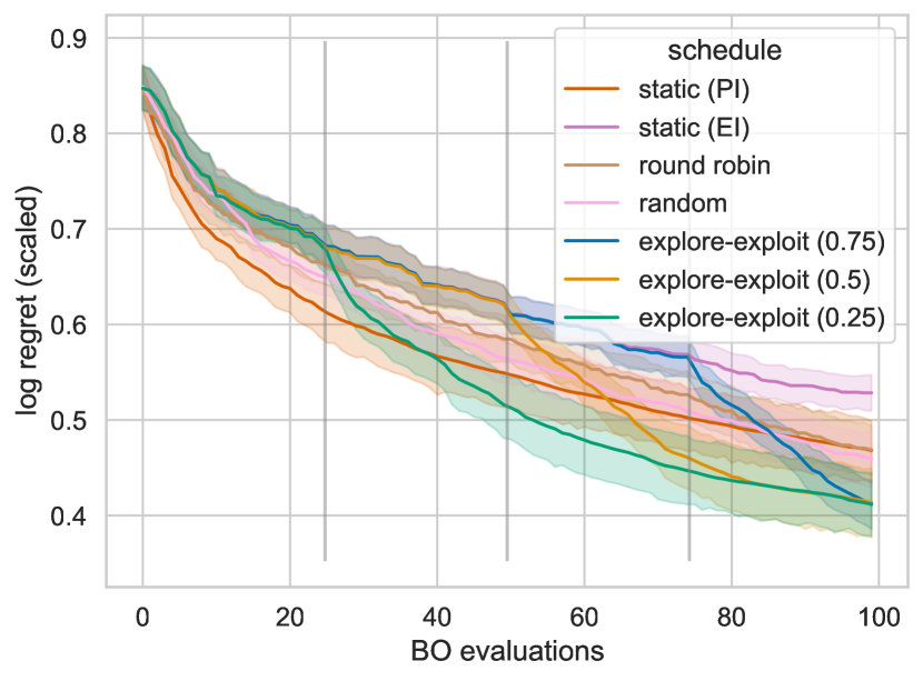
(b) Log-Regret (Scaled) per Step

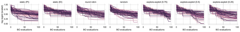
(c) Log-Regret (Scaled) per Step and Seed

Figure 14: BBOB Function 10

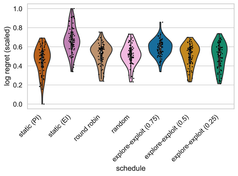
(a) Final Log Regret (Scaled)

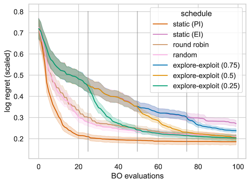
(b) Log-Regret (Scaled) per Step

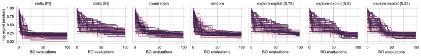
(c) Log-Regret (Scaled) per Step and Seed

Figure 15: BBOB Function 11

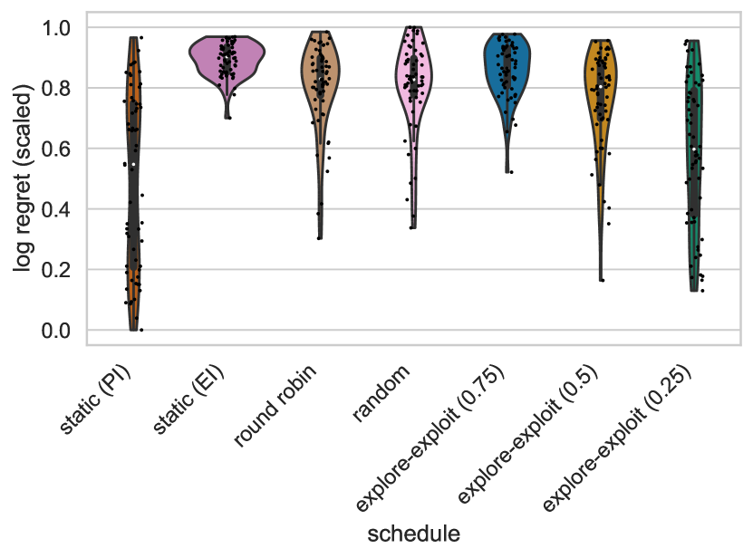
(a) Final Log Regret (Scaled)

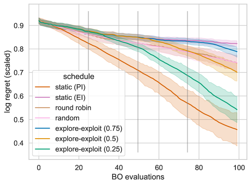
(b) Log-Regret (Scaled) per Step

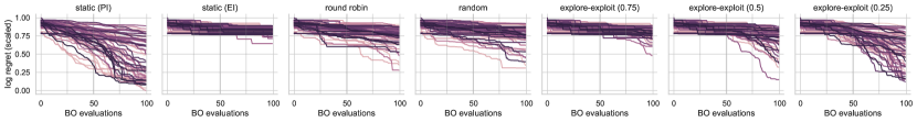
(c) Log-Regret (Scaled) per Step and Seed

Figure 16: BBOB Function 12

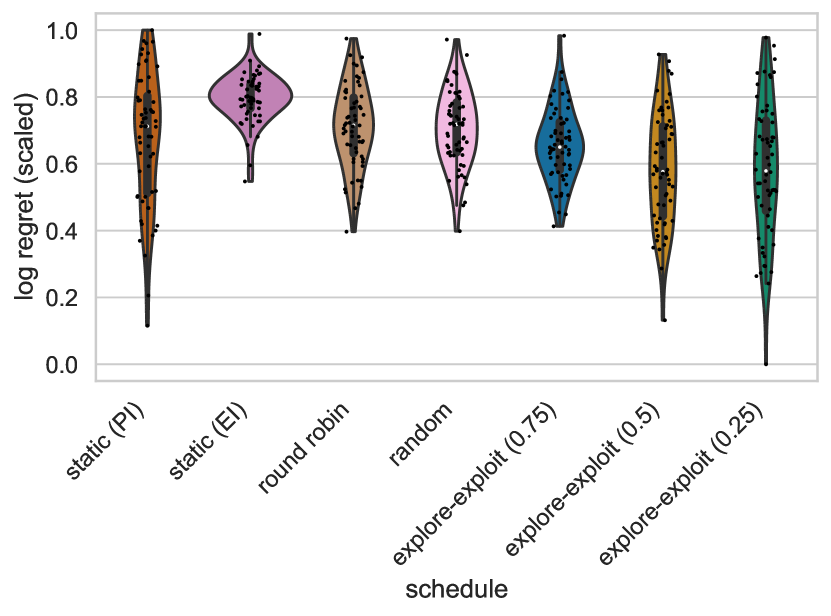
(a) Final Log Regret (Scaled)

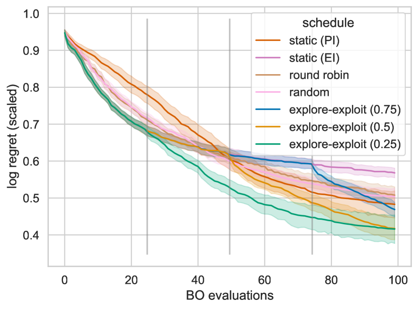
(b) Log-Regret (Scaled) per Step

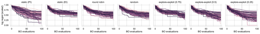
(c) Log-Regret (Scaled) per Step and Seed

Figure 17: BBOB Function 13

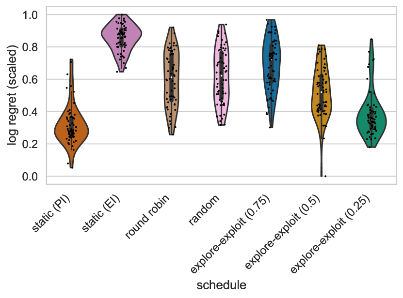
(a) Final Log Regret (Scaled)

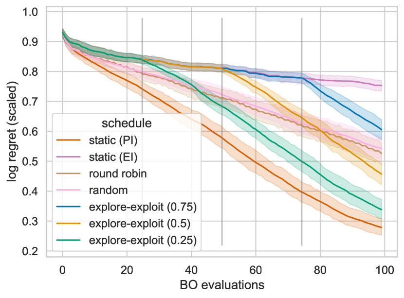
(b) Log-Regret (Scaled) per Step

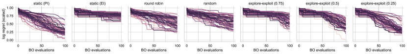
(c) Log-Regret (Scaled) per Step and Seed

Figure 18: BBOB Function 14

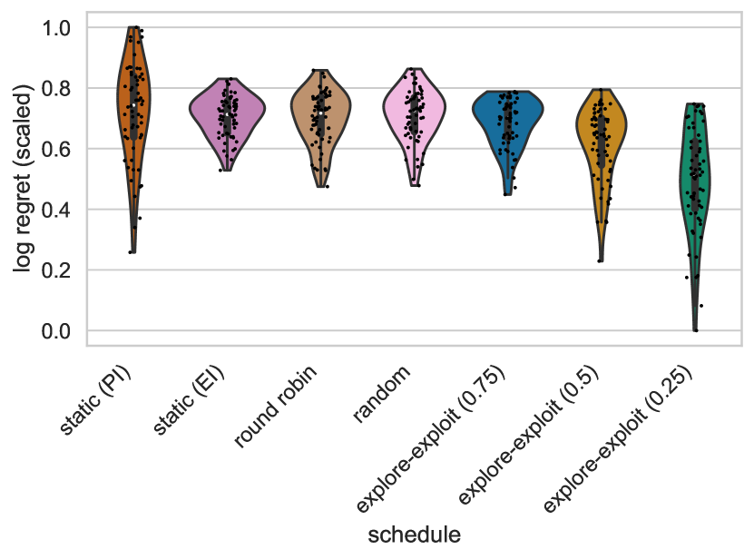
(a) Final Log Regret (Scaled)

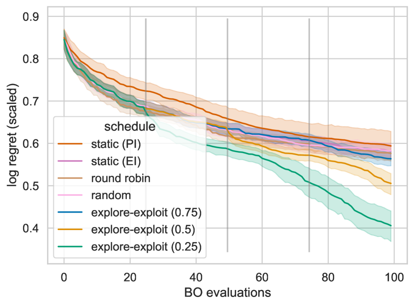
(b) Log-Regret (Scaled) per Step

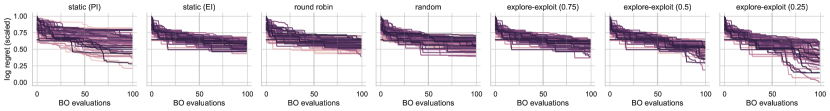
(c) Log-Regret (Scaled) per Step and Seed

Figure 19: BBOB Function 15

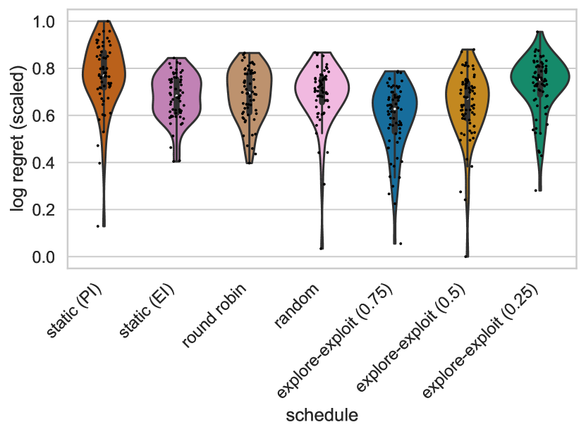
(a) Final Log Regret (Scaled)

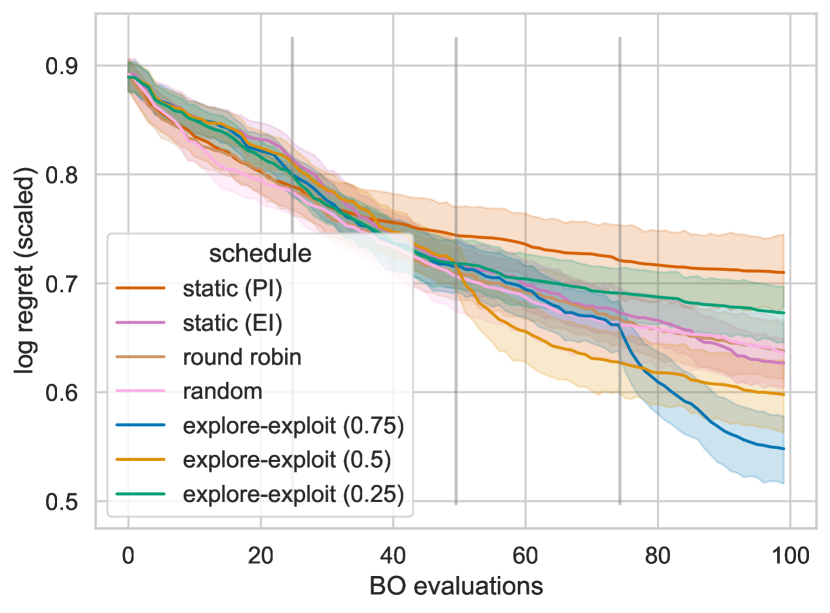
(b) Log-Regret (Scaled) per Step

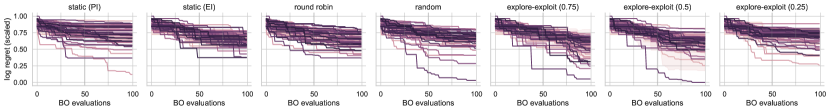
(c) Log-Regret (Scaled) per Step and Seed

Figure 20: BBOB Function 16

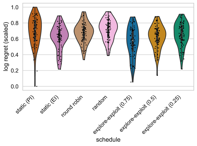
(a) Final Log Regret (Scaled)

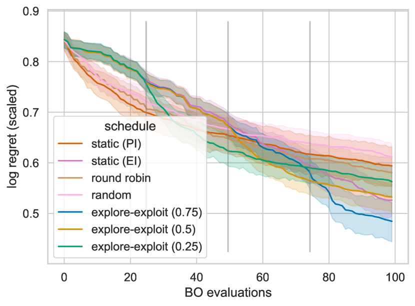
(b) Log-Regret (Scaled) per Step

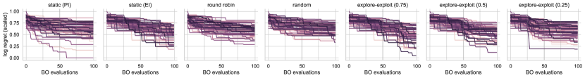
(c) Log-Regret (Scaled) per Step and Seed

Figure 21: BBOB Function 17

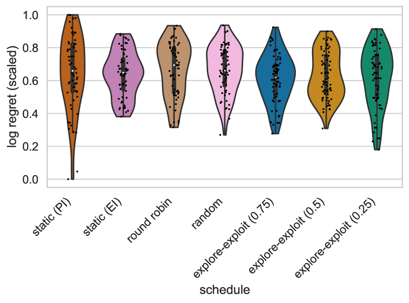
(a) Final Log Regret (Scaled)

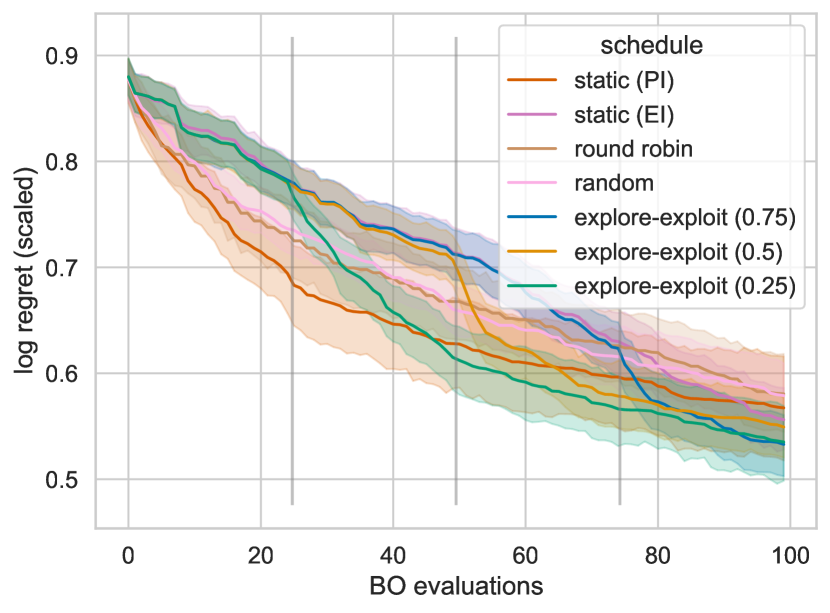
(b) Log-Regret (Scaled) per Step

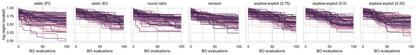
(c) Log-Regret (Scaled) per Step and Seed

Figure 22: BBOB Function 18

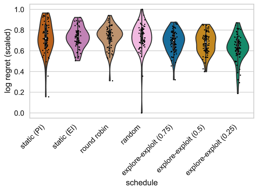
(a) Final Log Regret (Scaled)

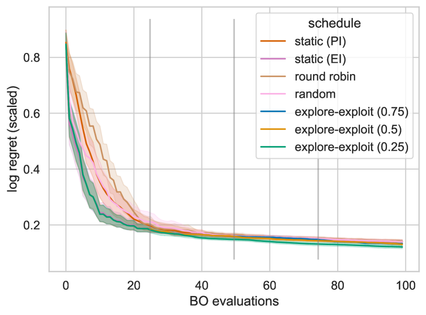
(b) Log-Regret (Scaled) per Step

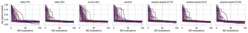
(c) Log-Regret (Scaled) per Step and Seed

Figure 24: BBOB Function 20

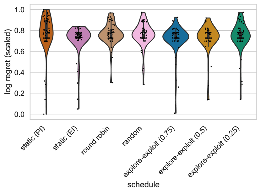
(a) Final Log Regret (Scaled)

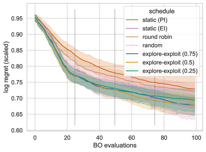
(b) Log-Regret (Scaled) per Step

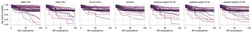
(c) Log-Regret (Scaled) per Step and Seed

Figure 25: BBOB Function 21

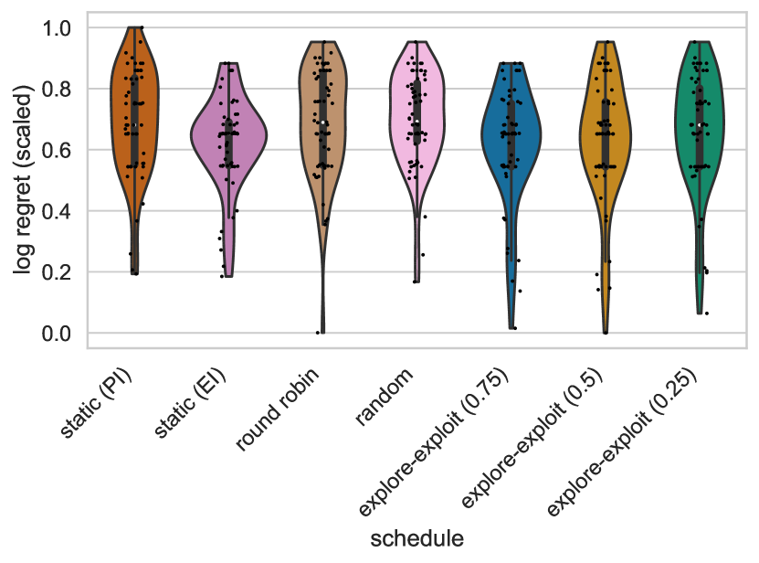
(a) Final Log Regret (Scaled)

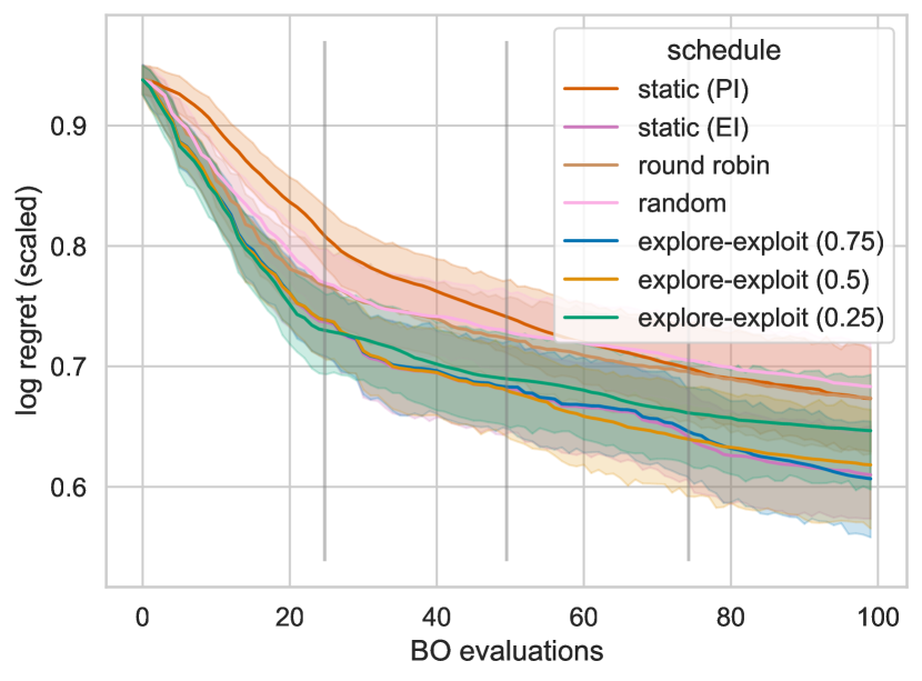
(b) Log-Regret (Scaled) per Step

(c) Log-Regret (Scaled) per Step and Seed

Figure 26: BBOB Function 22

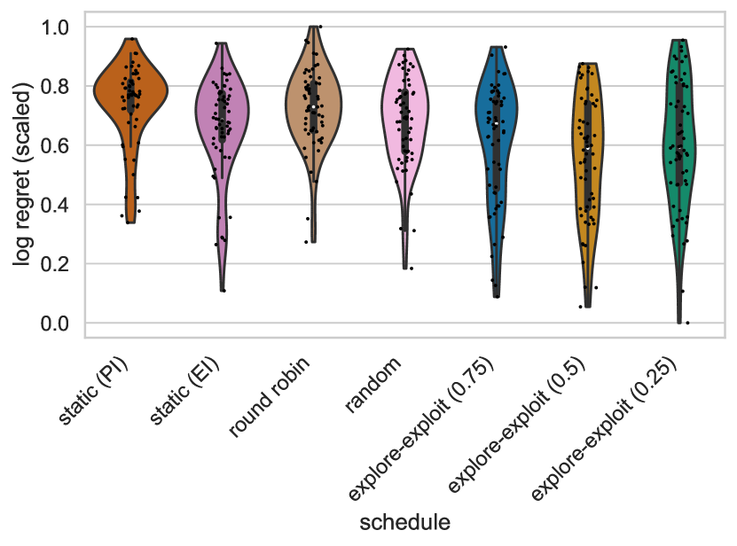
(a) Final Log Regret (Scaled)

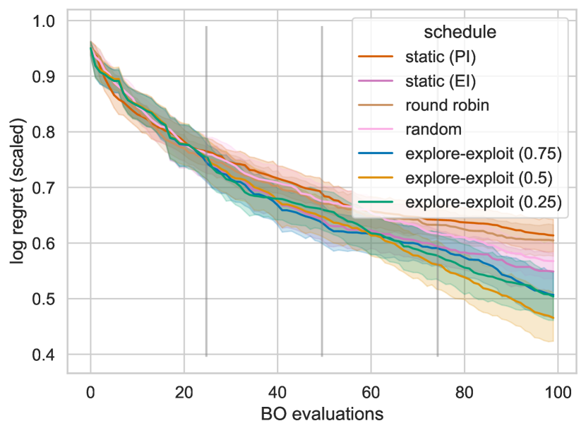
(b) Log-Regret (Scaled) per Step

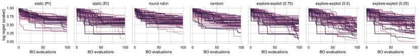
(c) Log-Regret (Scaled) per Step and Seed

Figure 28: BBOB Function 24

References

- Mockus [2012] Jonas Mockus. Bayesian Approach to Global Optimization: Theory and Applications. Springer Science & Business Media, December 2012. ISBN 978-94-009-0909-0.
- Lindauer et al. [2019] M. Lindauer, M. Feurer, K. Eggensperger, A. Biedenkapp, and F. Hutter. Towards assessing the impact of bayesian optimization’s own hyperparameters. In IJCAI’19 DSO Workshop, 2019.
- Cowen-Rivers et al. [2021] A. Cowen-Rivers, W. Lyu, R. Tutunov, Z. Wang, A. Grosnit, R. Griffiths, A. Maraval, H. Jianye, J. Wang, J. Peters, and H. Ammar. An empirical study of assumptions in Bayesian optimisation. arXiv:2012.03826 [cs.LG], 2021.
- Bossek et al. [2020] Jakob Bossek, Carola Doerr, and Pascal Kerschke. Initial design strategies and their effects on sequential model-based optimization: an exploratory case study based on BBOB. In Proc. of Genetic and Evolutionary Computation Conference (GECCO’20), pages 778–786. ACM, 2020. doi: 10.1145/3377930.3390155. URL https://doi.org/10.1145/3377930.3390155.
- Karafotias et al. [2015] G. Karafotias, M. Hoogendoorn, and Á. Eiben. Parameter control in evolutionary algorithms: Trends and challenges. IEEE Trans. Evolutionary Computation, 19(2):167–187, 2015.
- Doerr and Doerr [2020] Benjamin Doerr and Carola Doerr. Theory of parameter control mechanisms for discrete black-box optimization: Provable performance gains through dynamic parameter choices. In Theory of Evolutionary Computation: Recent Developments in Discrete Optimization, pages 271–321. Springer, 2020. doi: 10.1007/978-3-030-29414-4˙6. Also available online at https://arxiv.org/abs/1804.05650.
- Adriaensen et al. [2022] S. Adriaensen, A. Biedenkapp, G. Shala, N. Awad, T. Eimer, M. Lindauer, and F. Hutter. Automated dynamic algorithm configuration. arXiv:2205.13881 [cs.AI], 2022.
- Forrester et al. [2008] Alexander I. J. Forrester, András Sóbester, and Andy J. Keane. Engineering Design via Surrogate Modelling - A Practical Guide. John Wiley & Sons Ltd., 2008. ISBN 978-0-470-06068-1.
- Hansen et al. [2021] N. Hansen, A. Auger, R. Ros, O. Mersmann, T. Tušar, and D. Brockhoff. COCO: A platform for comparing continuous optimizers in a black-box setting. Optimization Methods and Software, 36:114–144, 2021. doi: 10.1080/10556788.2020.1808977.
- Qin et al. [2017] Chao Qin, Diego Klabjan, and Daniel Russo. Improving the expected improvement algorithm. In Isabelle Guyon, Ulrike von Luxburg, Samy Bengio, Hanna M. Wallach, Rob Fergus, S. V. N. Vishwanathan, and Roman Garnett, editors, Advances in Neural Information Processing Systems 30: Annual Conference on Neural Information Processing Systems 2017, December 4-9, 2017, Long Beach, CA, USA, pages 5381–5391, 2017. URL https://proceedings.neurips.cc/paper/2017/hash/b19aa25ff58940d974234b48391b9549-Abstract.html.
- Balandat et al. [2020] M. Balandat, B. Karrer, D. Jiang, S. Daulton, B. Letham, A. Wilson, and E. Bakshy. Botorch: A framework for efficient monte-carlo Bayesian optimization. In Proc. of NeurIPS’20, 2020.
- Volpp et al. [2020] M. Volpp, L. Fröhlich, K. Fischer, A. Doerr, S. Falkner, F. Hutter, and C. Daniel. Meta-learning acquisition functions for transfer learning in bayesian optimization. In Proc. of ICLR’20, 2020. URL https://openreview.net/forum?id=ryeYpJSKwr.
- Hoffman et al. [2011] Matthew Hoffman, Eric Brochu, and Nando de Freitas. Portfolio allocation for Bayesian optimization. In Proceedings of the Twenty-Seventh Conference on Uncertainty in Artificial Intelligence, UAI’11, pages 327–336, Arlington, Virginia, USA, 2011. AUAI Press. ISBN 9780974903972.
- Kandasamy et al. [2020] Kirthevasan Kandasamy, Karun Raju Vysyaraju, Willie Neiswanger, Biswajit Paria, Christopher R Collins, Jeff Schneider, Barnabas Poczos, and Eric P Xing. Tuning hyperparameters without grad students: Scalable and robust Bayesian optimisation with dragonfly. J. Mach. Learn. Res., 21(81):1–27, 2020.
- Thompson [1933] W. Thompson. On the likelihood that one unknown probability exceeds another in view of the evidence of two samples. Biometrika, 25(3/4):285–294, 1933.
- Speck et al. [2021] David Speck, André Biedenkapp, Frank Hutter, Robert Mattmüller, and Marius Lindauer. Learning heuristic selection with dynamic algorithm configuration. In Susanne Biundo, Minh Do, Robert Goldman, Michael Katz, Qiang Yang, and Hankz Hankui Zhuo, editors, Proceedings of the Thirty-First International Conference on Automated Planning and Scheduling, ICAPS 2021, Guangzhou, China (virtual), August 2-13, 2021, pages 597–605. AAAI Press, 2021. URL https://ojs.aaai.org/index.php/ICAPS/article/view/16008.
- Biedenkapp et al. [2020] A. Biedenkapp, H. F. Bozkurt, T. Eimer, F. Hutter, and M. Lindauer. Dynamic algorithm configuration: Foundation of a new meta-algorithmic framework. In Proc. of ECAI’20, pages 427–434, 2020.
- Hansen et al. [2003] N. Hansen, S. D. Müller, and P. Koumoutsakos. Reducing the time complexity of the derandomized evolution strategy with covariance matrix adaptation (CMA-ES). Evolutionary Computing, 11(1):1–18, 2003.
- Lindauer et al. [2022] M. Lindauer, K. Eggensperger, M. Feurer, A. Biedenkapp, D. Deng, C. Benjamins, T. Ruhkopf, R. Sass, and F. Hutter. SMAC3: A versatile bayesian optimization package for Hyperparameter Optimization. Journal of Machine Learning Research (JMLR) – MLOSS, 23(54):1–9, 2022.
- Mersmann et al. [2011] Olaf Mersmann, Bernd Bischl, Heike Trautmann, Mike Preuss, Claus Weihs, and Günter Rudolph. Exploratory landscape analysis. In Natalio Krasnogor and Pier Luca Lanzi, editors, 13th Annual Genetic and Evolutionary Computation Conference, GECCO 2011, Proceedings, Dublin, Ireland, July 12-16, 2011, pages 829–836. ACM, 2011. doi: 10.1145/2001576.2001690. URL https://doi.org/10.1145/2001576.2001690.