The Fifth Catalogue of Nearby Stars (CNS5)

Abstract

Context. We present the compilation of the Fifth Catalogue of Nearby Stars (CNS5), based on astrometric and photometric data from Gaia EDR3 and Hipparcos, and supplemented with parallaxes from ground-based astrometric surveys carried out in the infrared.

Aims. The aim of the CNS5 is to provide the most complete sample of objects in the solar neighbourhood. For all known stars and brown dwarfs in the 25 pc sphere around the Sun, basic astrometric and photometric parameters are given. Furthermore, we provide the colour-magnitude diagram and various luminosity functions of the stellar content in the solar neighbourhood, and characterise the completeness of the CNS5 catalogue.

Methods. We compile a sample of stars and brown dwarfs which most likely are located within 25 pc of the Sun, taking space-based parallaxes from Gaia EDR3 and Hipparcos as well as ground-based parallaxes from Best et al. (2021), Kirkpatrick et al. (2021), and from the CNS4 into account. We develop a set of selection criteria to clean the sample from spurious sources. Furthermore, we show that effects of blending in the Gaia photometry, which affect mainly the faint and red sources in Gaia, can be mitigated, to reliably place those objects in a colour-magnitude diagram. We also assess the completeness of the CNS5 using a Kolmogorov-Smirnov test and derive observational optical and mid-infrared luminosity functions for the main-sequence stars and white dwarfs in the solar neighbourhood.

Results. The CNS5 contains 5931 objects, including 5230 stars (4946 main-sequence stars, 20 red giants and 264 white dwarfs) and 701 brown dwarfs. We find that the CNS5 catalogue is statistically complete down to 19.7 mag in G-band and 11.8 mag in W1-band absolute magnitudes, corresponding to a spectral type of L8. The stellar number density in the solar neighbourhood is $(7.99\pm 0.11)\times 10^{-2}\,\text{stars pc}^{-3}$, and about 72% of stars in the solar neighbourhood are M dwarfs. Furthermore, we show that the white dwarf sample in CNS5 is statistically complete within 25 pc. The derived number density of white dwarfs is $(4.03\pm 0.25)\times 10^{-3}\,\text{stars pc}^{-3}$. The ratio between stars and brown dwarfs within 15 pc is $4.6\pm 0.4$, whereas within 25 pc it is $7.5\pm 0.3$. Thus, we estimate that about one third of brown dwarfs is still missing within 25 pc, preferentially those with spectral types later than L8 and distances close to the 25 pc limit.

1 Introduction

Hertzsprung (1922) was probably the first to notice that the systematic study of the stars in the solar neighbourhood is scientifically very valuable, for a multitude of reasons. First and foremost, the solar neighbourhood stars are the brightest (in terms of apparent magnitude) and largest (in terms of angular size) representatives of each spectral type, which allows us to observe them more easily while they can serve as proxies for more distant stars of the same type. Furthermore, the stellar sample in the solar neighbourhood provides the most complete census of the Galactic disc population, covering more than 20 mag in absolute visual brightness.

Often, the solar neighbourhood stars are used to develop concepts that are later applied elsewhere in the universe. Applications span a diverse range of astronomical topics, such as the number of stars in the Galaxy and Galactic disc modelling (Pritchet 1983; Bahcall 1986; Binney 2010; Just & Jahreiß 2010), the present-day and the initial mass functions (Miller & Scalo 1979; Rana & Basu 1992; Sollima 2019), the stellar luminosity function and its fine structure (Reid et al. 2002; Chabrier 2003; Bahcall 1986; Upgren & Armandroff 1981; Wielen et al. 1983; Kroupa et al. 1990; Jao et al. 2018), constraints on star formation (Kirkpatrick et al. 2019), the local stellar surface density (McKee et al. 2015), stellar multiplicity (Duquennoy & Mayor 1991; Dieterich et al. 2012), brown dwarfs (Meisner et al. 2020), and target lists for exoplanet searches (Reiners et al. 2018; Turnbull & Tarter 2003). This compilation is certainly not exhaustive; the cited works merely serve as an illustration of studies that have been conducted in each field. The solar neighbourhood sample hereby often complements other large photometric and spectroscopic datasets which have become available, such as RAVE (Steinmetz et al. 2020), SDSS (Ahumada et al. 2020), and PanSTARRS (Kaiser et al. 2002).

The number of surveys which are based on the nearby stars sample is expected to grow considerably in the future, especially due to the many endeavours to discover and characterise exoplanets. NASA has acknowledged the fact that many of the upcoming exoplanet search programs overlap in their target lists, especially for the nearby stars, and has established a working group (SAG 22) on the topic of a target star archive (Hinkel et al. 2021). Nearby stars possess several advantages over more distant stars as exoplanet hosts, such as better resolution for direct imaging (HabEx, Gaudi et al. 2020; LUVOIR, The LUVOIR Team 2019), or better stellar characterisation. Continued interest in the nearby stars sample is thus expected for the foreseeable future.

For these reasons we present here an update of the Catalogue of Nearby Stars, denoted CNS5. An update is well in order; since the publication of the Preliminary Version of the Third Catalogue of Nearby Stars (Gliese & Jahreiß 1991), a fourth version of the catalogue, CNS4, had been prepared by Hartmut Jahreiß, but never published.

While CNS4 was for the most part based on space-based parallaxes from Hipparcos (ESA 1997; van Leeuwen 2007a, b), CNS5 incorporates Gaia data (from the release Gaia EDR3, Gaia Collaboration et al. 2021a; Lindegren et al. 2021b). Due to Gaia’s superb astrometric precision and its large number of catalogue sources down to $G\sim 20$ mag and fainter, the completeness of the nearby star sample and the accuracy of astrometric and photometric parameters is tremendously improved. At the same time, the number of falsely included stars is also dramatically reduced.

As opposed to the recently published Gaia Catalogue of Nearby Stars (GCNS, Gaia Collaboration et al. 2021b), which lists all stars within 100 pc, the CNS5 sticks to its traditional volume of 25 pc around the Sun. CNS5 is not purely based on Gaia data, but also incorporates data from Hipparcos where favourable, as well as from CNS4 and from ground-based astrometric surveys carried out in the near-infrared. It aims for completeness and cleanliness of the final nearby stars sample to the extent possible, in order to facilitate statistical studies based on the volume-limited sample as a whole. In contrast, the GCNS includes all stars with a non-zero probability to lie within 100 pc, so it aims more at completeness rather than cleanliness near the distance limit. Naturally, completeness is higher in CNS5 compared to the GCNS, but this comes at the expense of a smaller volume. The applications of the two catalogues are thus to some extent complementary.

The compilation of the CNS5 is much more complicated than just selecting all sources with parallaxes larger than 40 mas. The reasons include a number of issues: i) spurious catalogue entries with apparently large parallaxes (Lindegren et al. 2021b; Gaia Collaboration et al. 2021b) which have to be filtered out, ii) blended sources whose photometry has to be deblended so that they can be reliably placed into a Hertzsprung-Russell diagram, and iii) the various components of multiple systems which have to be treated in a consistent way, even if reliable parallaxes do not exist for all of the components. Furthermore, we do not only use Gaia EDR3, but also the Hipparcos Catalogue (ESA 1997) for the brighter stars missing in Gaia as well as ground-based infrared parallax surveys (Best et al. 2021; Kirkpatrick et al. 2021) for the red and optically faint objects such as brown dwarfs. We also derive completeness limits and white dwarf and main-sequence star luminosity functions.

The paper is organised as follows. In Sect. 2 we describe various other catalogues of nearby stars, both previous and current. In Sect. 3 we present the philosophy behind the compilation of the CNS5 as well as our methods. Section 4 provides a description of the catalogue content, while Sect. 5 addresses completeness limits as well as the luminosity function; it also presents the colour-magnitude diagram (CMD) of all catalogue stars. Section 6 provides our conclusions and a summary. Detailed descriptions of algorithms are provided in the appendices.

2 Overview of the catalogues of nearby stars

2.1 Catalogue of Nearby Stars Series (CNS)

2.1.1 Previous editions

The first version of the Catalogue of Nearby Stars (CNS1) was published by Gliese (1957); it contained 1094 stars (915 systems) within 20 pc. The subsequent update of the catalogue (CNS2) expanded the coverage to 22.2 pc and contained 1627 stars in 1313 systems (Gliese 1969). It lists photometric, spectroscopic and trigonometric parallaxes as well as the ‘resulting parallax’, an estimate of the best value considering all measurements.

CNS3, entitled Preliminary Version of the Third Catalogue of Nearby Stars, lists 3403 stars within the 25 pc distance limit (Gliese & Jahreiß 1991). In contrast to CNS2, the resulting parallax in CNS3 is the trigonometric parallax, unless it is either not available or has unusually large errors. Although this version of the catalogue was denoted as ‘preliminary’, it is still the most recent publicly available edition of the CNS (a ‘final’ version was never published). Therefore, many recent publications are still based on the CNS3 (e.g. Tamazian & Malkov (2014); Bar et al. (2017); Price et al. (2020) to name a few).

The 4th version (CNS4) was created by Jahreiß & Wielen (1997). It contained ground-based parallaxes as well as trigonometric parallaxes from Hipparcos. However, the data from previous versions of the CNS series was not fully homogenised with the new data, which lead to inconsistencies.

Over decades, one of us (Hartmut Jahreiß) has continuously scanned the literature to update astrometry, photometry and other supplementary data (radial velocities, binary information) of potential nearby stars. This information has also been used in the construction of the CNS5.

2.1.2 Numbering scheme in the CNS

Stars in the CNS1 were designated as  Gl NNN, where NNN represents the consecutive integer number ordered by right ascension. In the CNS2 designations were formatted as  Gl NNN.N, adding a decimal place for the new stars. This allowed the original Gliese star numbers to be preserved and the ordering system by right ascension to be kept.

Since the publication of an extension to CNS2 (Gliese & Jahreiß 1979), the stars were referred to as  GJ NNNN. In addition, the CNS3 had listed Woolley numbers (Woolley et al. 1970) and introduced NN designations for new stars; both of them have been replaced with GJ numbers in the mean time. By now, all the previously known nearby stars thus have GJ designations. One can still tell from where they originated by their number: Woolley numbers start at 9001 and the largest assigned number is 9850, while NN numbers range from 3001 to 4388. The widely used Gliese-Jahreiß (GJ) numbers have been kept in the CNS5 (see Sect. 4.1 for details).

2.2 Other catalogues

2.2.1 The RECONS project

The REsearch Consortium On Nearby Stars (RECONS; founded in 1994) has made an enormous effort to discover and characterise stars and ultra-cool dwarfs in the 25 pc volume, primarily by measuring their trigonometric parallaxes from the ground (e.g. Henry et al. 2018). They provided updated astrometric, photometric and multiplicity information, and identified many new nearby stars since the publication of the Yale Parallax Catalog (van Altena et al. 1995). Their results are published in The Solar Neighborhood series of papers in The Astronomical Journal (49 papers as of June 2022), making the compilation of the 25 pc sample from their work rather cumbersome. Only statistics for the 10 pc volume is given on their website. As of 2018, the RECONS database contained 317 systems within 10 pc. An overview of new nearby stars within 10 pc discovered by RECONS is provided in Henry et al. (2018).

2.2.2 Catalogue of stars within 50 pc based on Gaia DR2

Torres et al. (2019) studied the dynamical evolution of the comets in the Oort cloud. In particular, they characterised stellar encounters with the Solar System by integrating their orbits based on Gaia DR2 data. For this purpose, the catalogue of stars within 50 pc based on Gaia DR2 data has been constructed. The catalogue lists 14 659 stars.

However, the approach used for source selection is a potential concern. Sources with high-quality astrometry were selected based on the relative uncertainty of the parallax (smaller than 20%), flux excess factor, and unit weight error ($UWE$). The re-normalisation of $UWE$ ($RUWE$; Lindegren 2018) was not incorporated when selecting sources for the catalogue. Such re-normalisation would preserve objects with extreme colours (e.g. such as brown dwarfs) from being removed because, contrary to $UWE$, not only is the object’s $G$ magnitude taken into account when calculating $RUWE$, but also its colour.

As the authors pointed out themselves, the catalogue is incomplete. The prime culprit here is the Gaia magnitude limit and, as a consequence, a significant number of faint low-mass stars is not detected. Furthermore, some of the brightest sources are also missing due to the Gaia saturation limit.

2.2.3 GCNS

The GCNS (Gaia Collaboration et al. 2021b) aims to identify all sources in Gaia EDR3 with reliable astrometry and a non-zero probability of being located within 100 pc from the Sun. This is done by retrieval of sources with parallaxes larger than 8 mas, removal of spurious sources with machine-learning (using the random forest classifier) and by Bayesian distance estimation for the remaining sources.

The full catalogue lists 331 312 sources. The overall completeness of the GCNS is expected to be 95% or better for spectral types up to M8 (translating into $M_{G}=15.7\leavevmode\nobreak\ {\rm mag}$).

It is important to bear in mind that the prime focus of the GCNS is to provide a homogeneous census of nearby stars. Its volume is larger than that of the CNS5, but bright and red sources could be missing since the GCNS is based only on Gaia EDR3 data. As we will see, due to the inclusion of infrared surveys in the CNS5, the CNS5 is complete for much later spectral types well into the brown dwarf regime.

2.2.4 The 10 pc sample by Reylé et al. (2021)

Reylé et al. (2021) compiled the sample of stars, brown dwarfs, and exoplanets located within 10 pc of the Sun as a quality assurance test for the GCNS. Using this sample, it is possible to not only identify very nearby stars that are missing from the GCNS (or future Gaia data releases), but also infer the completeness of the GCNS by estimating the expected number of objects of different types from the number densities for the 10 pc volume.

Objects for the 10 pc sample were selected from SIMBAD using a strict cut on parallax at $\geq 100$ mas, with parallax uncertainties playing no role in the selection process. The sample was supplemented with components of unresolved binaries, brown dwarfs with recently published parallaxes from Best et al. (2021) and Kirkpatrick et al. (2019, 2021), and confirmed exoplanets from the Extrasolar Planets Encyclopædia as well as from the NASA Exoplanet Archive.

The sample consists of 540 objects (including 77 exoplanets) in 339 systems. The Sun and its planets are not included. The 10 pc sample has separate entries for every object, including the unresolved components of multiple systems and exoplanets.

Naturally, among the catalogues reviewed in this section, the 10 pc sample by Reylé et al. (2021) has the highest completeness due to its smaller volume. At the same time, the number of objects contained within this volume is insufficient for statistical studies of the solar neighbourhood.

Future updates of the 10 pc sample are anticipated to have only a minor impact on the stellar content of the sample; the majority of the new additions to the sample are expected to come from single stars that have been resolved into multiple components. In the substellar regime, the expected additions will be ultra-cool dwarfs (particularly those in the Galactic plane) and, of course, new exoplanets.

3 Construction of the CNS5 catalogue

3.1 Data selection

Our goal for the compilation of the CNS5 is to maximise completeness within the 25 pc limit. Therefore, the wealth of data from several different catalogues and surveys has to be carefully selected and combined. In the following subsections we give a full account of our selection criteria, applied corrections, and how we combined data from the different catalogues to consolidate the CNS5.

3.1.1 Gaia EDR3

Due to its high completeness and high accuracy Gaia EDR3 is an excellent starting point for the preparation of a catalogue of nearby stars. For the vast majority of objects the Gaia parallax clearly indicates whether the star is located within 25 pc from the Sun or not. Therefore, CNS5 is built primarily based on the data selected from Gaia EDR3 and then, if necessary, supplemented with data from Hipparcos and other catalogues and sources.

The primary sample for CNS5 is constructed by retrieving from Gaia EDR3 all the objects that are possibly located within 25 pc from the Sun:

$$\varpi_{\rm EDR3}-Z_{5,6}+3\eta\sigma_{\varpi}{}_{\rm EDR3}\geq 40\leavevmode\nobreak\ \text{mas},$$ (1)

where $\varpi$_EDR3 denotes the measured parallax in the Gaia EDR3 catalogue, $\sigma_{\varpi}$_EDR3 its standard error, $Z_{5,6}$ is the parallax zero-point for the five and six parameter solutions in Gaia EDR3, and $\eta$ is the parallax error inflation factor. The parallax zero-point correction and the inflation factor for the parallax error will be discussed below. The query returns 5876 sources.

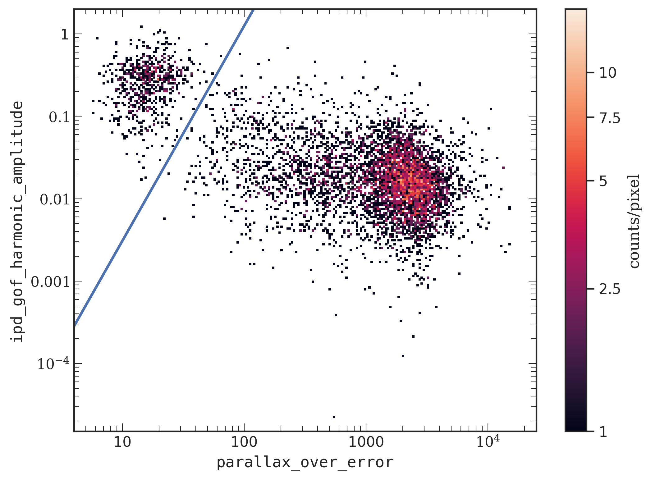
Figure 1: Dichotomy between sources with spurious and reliable astrometric solutions. The blue line corresponds to Eq. (2); 692 sources (11.78%) are located above this threshold and hence their astrometric solutions are spurious.

Sources with spurious astrometric solutions are removed by applying a simple yet powerful cut on the amplitude of the Image Parameter Determination goodness-of-fit (IPD GoF; ipd_gof_harmonic_amplitude in Gaia EDR3). Thus, we construct our sample by retaining only sources that satisfy the following condition:

$$A_{\rm GoF}<10^{-5.12}(\varpi_{\rm EDR3}/\sigma_{\varpi}{}_{\rm EDR3})^{2.61},$$ (2)

where $A_{\rm GoF}$ is the amplitude of the IPD GoF.

Figure 1 shows that sources with spurious solutions and nearby sources with good parallaxes form two distinct groups in (ipd_gof_harmonic_amplitude, parallax_over_error) parameter space and are separated by Eq. (2). This cut is discussed and validated in detail in Appendix A.

One of the strengths of this cut is that the photometric parameters themselves are not involved in the selection process. This is opposed to other widely used selection criteria such as $RUWE$, where the re-normalisation factor is a function of the $G$-band magnitude and the $BP-RP$ colour (Lindegren 2018) or the photometric excess factor, which is based solely on photometry (Evans et al. 2018; Lindegren et al. 2018). By filtering with Eq. (2) we avoid introducing a selection bias against, for instance, variable stars. It has been shown that an excess in $RUWE$ can be induced not only by binarity of an object but also by its photometric variability (Belokurov et al. 2020). Such a source is observed at a broad range of magnitudes (and sometimes even colours) and consequently this affects the $RUWE$ re-normalisation coefficient, which is derived assuming constant apparent magnitudes. The photometric excess factor must be interpreted with caution too: while it is common to use it as a data quality indicator to identify issues with crowding or background subtraction, it is important to bear in mind that variable sources frequently have large values of flux excess as well (Riello et al. 2021).

It is important to bear in mind that our cut, in principle, may reject a few unresolved or marginally resolved binaries. However, the number of rejected objects should be negligible and probably comes down to the 12 objects listed in Table 5. Furthermore, we do not know the true parallaxes of these objects since their astrometric solution (which is based on the assumption of the single-star model) might be affected by binarity. Thus, it is not clear whether these objects even belong to the 25 pc volume.

Parallaxes published in Gaia EDR3 are known to be underestimated by a few tens of microarcseconds, and a correction of this systematic parallax offset is needed (Lindegren et al. 2021a). In this paper it has also been demonstrated that the parallax zero-point correction (parallax bias) depends on the G magnitude of the object, its colour and ecliptic latitude $\beta$.

We would like to stress that the parallax zero-point correction is not negligible for nearby stars, even though their parallaxes are several orders of magnitude larger than the parallax zero-point offset. It has been shown by Bailer-Jones that the distances in the GCNS are overestimated on average by 0.22 pc, and the dominant cause for this difference is that GCNS does not incorporate a correction for the parallax zero-point offset.

We computed parallax zero-point values for each source in our sample from Gaia EDR3 according to the procedure of Lindegren et al. (2021a) and subtracted it from the parallax value published in Gaia EDR3. 16 sources would not have been part of the CNS5 sample if we had not applied the parallax zero point, so the correction is not only important for deriving the most accurate distances but also sample selection and its completeness.

Regarding the parallax uncertainties in Gaia EDR3, several studies validated them using different approaches and have shown that the uncertainties are underestimated (El-Badry et al. 2021; Fabricius et al. 2021; Maíz Apellániz et al. 2021; Vasiliev & Baumgardt 2021; Zinn 2021). We inflated parallax errors in our sample using an empirical function for the inflation factor derived in El-Badry et al. (2021). It is important to bear in mind that the inflation factor must be interpreted as a lower limit. The underestimation of the parallax uncertainty is even larger for sources with large $RUWE$ values, binaries with small angular separation, and for sources in the vicinity of other bright sources. For the bright stars outside the interpolation region $7\leavevmode\nobreak\ {\rm mag}<G<21\leavevmode\nobreak\ {\rm mag}$, we have decided to also inflate the parallax uncertainties, given that for $2\leavevmode\nobreak\ {\rm mag}<G<7\leavevmode\nobreak\ {\rm mag}$ the inflation function is well-behaved and flattens towards a constant value of $\sim 1.15$ . By doing so, we ensure that the parallax uncertainty distribution remains continuous within the whole magnitude range $2\leavevmode\nobreak\ {\rm mag}<G<21\leavevmode\nobreak\ {\rm mag}$. Consequently, this will yield more accurate and consistent results in astrophysical applications of our catalogue.

Six objects in the CNS5 would not have been included if the parallax errors would not have been inflated. These objects all have $G$ magnitudes in the range $11.03\leavevmode\nobreak\ {\rm mag}\leq G\leq 15.35\leavevmode\nobreak\ {\rm mag}$, so that they are well within the interpolation region $7\leavevmode\nobreak\ {\rm mag}<G<21\leavevmode\nobreak\ \leavevmode\nobreak\ {\rm mag}$ of Eq. (16) in El-Badry et al. (2021).

The parallaxes from Gaia DR2 were not considered during the data selection process, and there are several reasons that justify this decision. Typically, the parallax uncertainties in Gaia EDR3 are smaller by a factor 0.8 or better than in Gaia DR2 due to improved calibrations and the longer time span of the observations: Gaia DR2 is based on 22 months of observations while Gaia EDR3 is based on data collected during 34 months (Lindegren et al. 2021b). In a few cases, the opposite is true and, despite the longer time span of the observations, the parallax uncertainty is larger in Gaia EDR3. This can often be a consequence of the object being an unresolved binary with the orbital period comparable with the Gaia EDR3 temporal baseline. Over time, the contribution of the orbital motion accumulates and can induce a photocentre perturbation. This leads to the significant inconsistency of the observed displacement of the source with the single-star model fit, which in turn translates into increased uncertainties of parallaxes and proper motions.

Furthermore, we have decided against adding new objects with the parallaxes from Gaia DR2 which have just two-parameter solutions in Gaia EDR3 or are missing completely. The vast majority of such sources have spurious solutions in Gaia DR2 and did not meet the acceptance criteria during reprocessing in Gaia EDR3 (Lindegren et al. 2021b). Including these sources would thus contaminate our catalogue. We would like to remark that sources with spurious solutions in Gaia DR2 cannot be eliminated with our criterion in Eq. (2) since the IPD GoF statistics are not included in that data release. Finally, it appears not to be feasible to construct a volume-limited sample of nearby stars based on Gaia DR2 which would be free from spurious entries and at the same time without removing too many real sources. As we outlined above, the widely used selection criteria – namely $RUWE$ and the photometric excess factor – are sub-optimal for this task. Alternatively, applying machine-learning will not necessarily provide a classification which is robust enough. As reported in Gaia Collaboration et al. (2021b), when the same random forest classifier as the one which was used to construct the GCNS has been applied to Gaia DR2 (but with the predictive variables adapted to those available in Gaia DR2), the resulting sample still contained 15 sources with $\varpi>500\ \mathrm{mas}$, whereas in Gaia EDR3 there are only two such sources – Barnard's star and Proxima Centauri.

3.1.2 Hipparcos

While Gaia EDR3 includes the majority of known nearby stars, it is certainly not complete, as in particular the very brightest stars are missing. As the next step, we thus supplemented our Gaia EDR3 sample with entries from the Hipparcos Catalogue (Perryman et al. 1997), which is complete for $V$ magnitudes brighter than 7.3–9.0 mag. By doing so, we add objects which are too bright for Gaia and thus missing, or which do not have a full astrometric solution in Gaia EDR3. Furthermore, Gaia EDR3 is also incomplete for high proper motion stars: $\sim 8\%$ of known stars with proper motions $\gtrsim 0.6\leavevmode\nobreak\ \mbox{arcsec\,yr}^{-1}$ are missing in Gaia EDR3 (Fabricius et al. 2021). Another major advantage of including data from Hipparcos is that for very bright objects it usually provides astrometry of higher quality than the one from Gaia EDR3.

Similar as for the selection of stars from Gaia EDR3, objects from the Hipparcos Catalogue were selected based on their parallax. In addition, we impose an upper limit on parallax error to avoid adding objects with extremely large parallax uncertainties, which often result from photocentre wobble of unresolved or marginally resolved binaries:

$$\left.\begin{aligned} \text{(i)}\quad&\varpi+3\sigma_{\varpi}{}\geq 40\leavevmode\nobreak\ \text{mas}\\ \text{(ii)}\quad&\sigma_{\varpi}{}\leq 10\leavevmode\nobreak\ \text{mas}\end{aligned}\quad\right\},$$ (3)

where $\varpi$ is the parallax from the Hipparcos Catalogue and $\sigma_{\varpi}$ its formal error. In this paper we use the second reduction of the Hipparcos astrometric catalogue with improved parallaxes and their formal errors (van Leeuwen 2007a, b). The selected sample contains 2 007 sources. We adopted the cross-match with Gaia EDR3 provided by Marrese et al. (2021a), described in Marrese et al. (2021b).

A comparison of parallax errors from Hipparcos and Gaia EDR3 shows that for objects fainter than $G\,{\approx}\,6$ mag the Gaia EDR3 parallaxes typically have one to two orders of magnitude higher precision than those measured by Hipparcos. However, parallaxes from Hipparcos for very bright objects have smaller standard errors, due to the saturation limit of Gaia. Figure 2 shows the ratio of parallax errors from Hipparcos and inflated errors from Gaia EDR3 ($\sigma_{\varpi}$_HIP/$\eta$$\sigma_{\varpi}$_EDR3) as a function of the Gaia $G$-band magnitude. Here we found that for the objects brighter than $G\approx 4$ mag Hipparcos parallaxes are typically better (i.e.  $\sigma_{\varpi}$_HIP/$\eta$$\sigma_{\varpi}$_EDR3 $<1$). Therefore, the parallax values with the smaller uncertainties ($\sigma_{\varpi}$_HIP or $\eta$$\sigma_{\varpi}$_EDR3) will be adopted as a resulting parallax in the CNS5 for those objects which are present in both catalogues, Gaia EDR3 and Hipparcos.

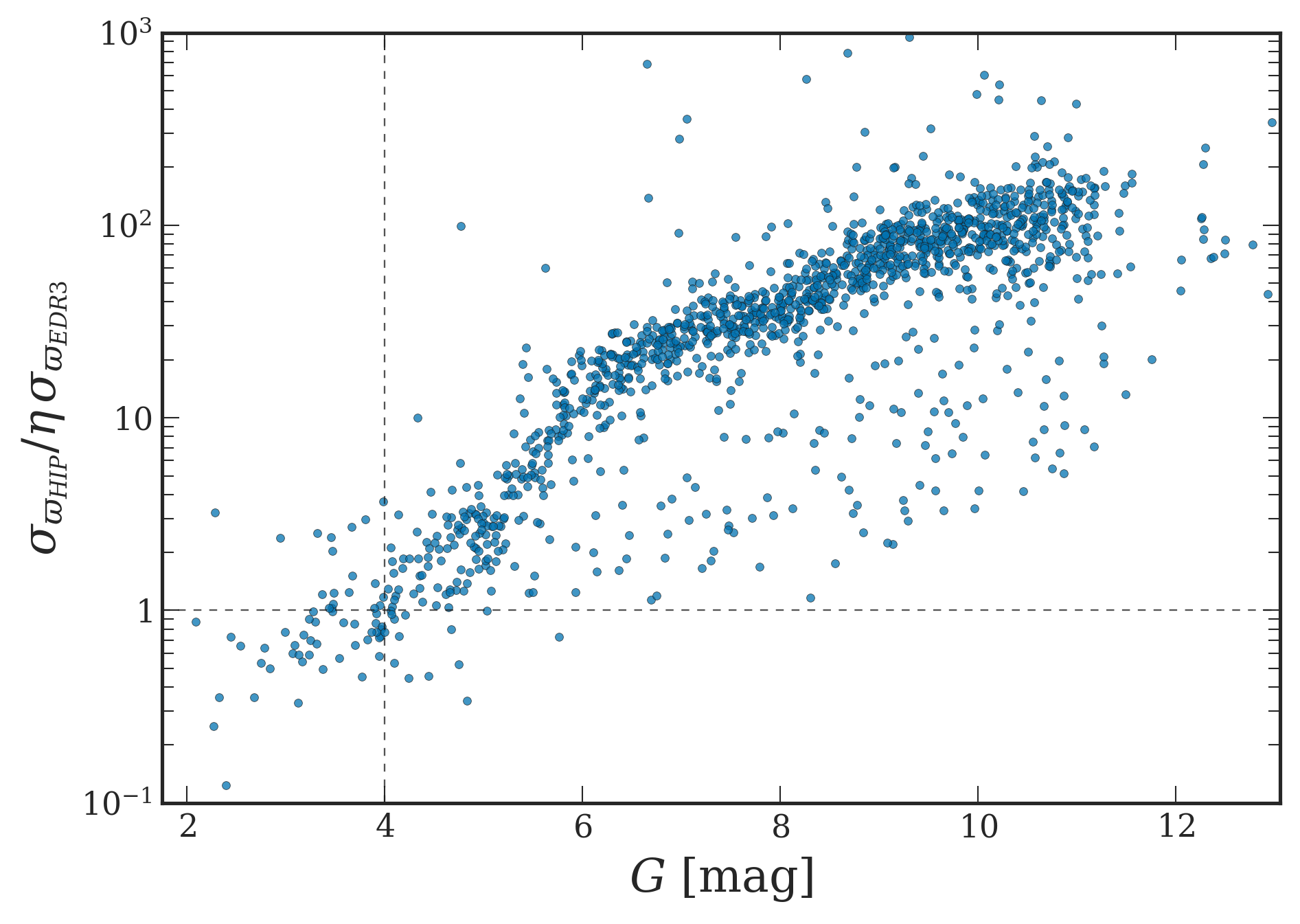
Figure 2: Ratio of parallax errors in the Hipparcos and Gaia EDR3 catalogues as a function of $G$ magnitude. Parallax errors from Gaia EDR3 are the inflated ones. For the objects brighter than $G\approx 4$ mag (vertical dashed line) parallax uncertainties in Hipparcos are typically smaller than those from Gaia EDR3.

3.1.3 Ultra-cool dwarfs

Objects fainter than the Gaia magnitude limit of 20–21 mag in $G$ band are so far missing from our sample. This concerns many of the L and T dwarfs in the 25 pc volume. Thus we decided to add nearby ultra-cool dwarfs from the compilation by Best et al. (2021), who recently provided a sample which is complete within 25 pc for spectral types from L0 to T8. All stars in their sample have parallaxes, many of them measured as part of the Hawaii Infrared Parallax Program (Dupuy & Liu 2012, and later papers in the series). As the next step, we updated and supplemented the resulting sample with Spitzer parallaxes from Kirkpatrick et al. (2021).

As usual, we included only objects that are possibly within the 25 pc volume according to Eq. 3 and discarded those objects with parallax errors larger than 10 mas. Again, only trigonometric parallaxes were considered. This resulted in a sample of 906 objects. Typical parallax errors in the resulting sample of ultra-cool dwarfs range from 1 to 10 mas, larger than those from Hipparcos and Gaia, as can be seen in Fig. 6. Nevertheless, adding the ultra-cool dwarfs helps tremendously with completeness towards the smallest masses. In total, 462 ultra-cool dwarfs without counterparts in Gaia EDR3 were added to the CNS5 from the sample of Best et al. (2021) and 79 from the sample of Kirkpatrick et al. (2021).

3.1.4 CNS4

We add sources from the internal version of the CNS4 which are missing so far in our sample from Gaia EDR3, Hipparcos and Best et al. (2021). This is done by identifying and discarding those objects in CNS4 that (i) are already included in our sample, (ii) now have higher-precision parallax measurements that move them outside the 25 pc limit, (iii) were classified as a nearby star in the past, whereas newer studies showed that they actually have non-stellar nature such as, for instance, a plate flaw (GJ~2087) or even BL Lac objects (GJ~3750 and GJ~3848), (iv) are sources listed as a component of a nearby star, whereas newer studies could not confirm them, concluded that they are non-existing or showed that they are not physically bound and therefore are background stars, (v) have trigonometric parallaxes with errors exceeding an upper limit of $10\leavevmode\nobreak\ \text{mas}$, (vi) have only photometric parallax measured.

Cross-matching CNS4 with our sample was often compounded by inconsistencies in the CNS4 between listed designations and coordinates, which were not always up to date. Such cases had to be handled manually and frequently required significant amounts of detective work.

For every object retained in the resulting sample, we collected updated astrometry from the literature and supplemented it with optical, NIR and MIR photometry whenever possible. Our attempts to identify a counterpart in Gaia EDR3 with a two parameter solution were successful for objects predominantly of intermediate brightness, whereas an unambiguous identification of Gaia EDR3 counterparts for fainter objects was often stymied by the presence of two or more sources of similar brightness (and with only a two parameter solution in Gaia EDR3 for them) in the vicinity. Confident cross-matching with Gaia EDR3, even when only a two parameter solution was available, provides not only highly accurate coordinates but also photometry in the Gaia bands. When combined with parallaxes from the literature, this allows to reliably place these sources in the CMD.

The objects added from the CNS4 are typically M dwarfs of intermediate brightness with only a two parameter solutions in Gaia EDR3. The additional 27 objects from CNS4 are crucial to maximise completeness of the CNS5.

Table 1: GJ~559 and GJ~551 as an example for indexing binary and multiple systems in the CNS5.

cns5_id	gj_id	component_id	n_components	gj_system_primary
CNS5 3591	551	C	3	559
CNS5 3628	559	AB	3	-

3.2 The Sun

As was pointed out in the introduction, the aim of the CNS5 is to provide the most complete census of nearby stars possible, so that it can be used for statistical studies of the solar neighbourhood. Thus, there is no strong reason not to include the nearest star - the Sun. On the other hand, due to its proximity, its treatment is different from that of other stars in the catalogue, and a few notes have to be made here.

In the catalogue entry for the Sun we list only apparent magnitudes in different photometric bands. Consistent with previous versions of the CNS catalogues, we do not assign any GJ designation to this entry.

Traditionally, the distance between the Sun and Earth (and thus absolute magnitudes of the Sun) was estimated from the solar parallax. The determination of the solar parallax has been a fundamental problem in observational astronomy over the centuries (Bond 1857; Tupman 1878; Hinks 1909; Turner 1912; Weaver 1943; Thomson et al. 1961). For an overview of principles of the determination of the solar parallax with Gaia please refer to Mignard (2020). However, since 2012 the Astronomical Unit (au) is a conventional unit of length and equals exactly 149 597 870 700 m (translating to the solar parallax of $\varpi_{\odot}=8.794143836\arcsec$), as defined by IAU (2012). Given that the stellar parallax is non-definable for the Sun and that our catalogue only lists trigonometric stellar parallaxes, no parallax value is given for the Sun.

Turning now to photometry, the solar magnitudes and colours serve as an important reference point in many areas of astrophysics. However, we do not have a measured value of neither $G_{\sun}$, nor its colours $(G-RP)_{\sun}$ or $(BP-RP)_{\sun}$. The approach to be taken here is to use magnitudes and colours estimated from flux calibrated solar reference spectra. Casagrande & VandenBerg (2018) reported magnitudes of the Sun in the Gaia bands in the Vegamag system derived from absolute flux measurements, both ground-based and from space, combined with model spectra. Hence, we adopt $G_{\sun}=-26.90$ mag (this corresponds to an absolute magnitude of $M_{G_{\sun}}=4.67$ mag), $(G-RP)_{\sun}=0.49$ mag and $(BP-RP)_{\sun}=0.82$ mag for the Sun.

Similarly, Willmer (2018) estimated the apparent and absolute magnitudes of the Sun in a large number of other broad-band filters used in various surveys and observatories. Thus we tabulate in the CNS5 the NIR and MIR magnitudes of the Sun, that is, in 2MASS ($J,H,K_{s}$) and WISE ($W_{1},W_{2},W_{3},W_{4}$) filters. We remark that the magnitudes of the Sun listed in the CNS5 are in the Vegamag system.

4 Description of the catalogue

4.1 Numbering scheme

All objects in the catalogue are designated in the format $\textbf{CNS5}\leavevmode\nobreak\ NNNN$, where $NNNN$ represents the sequence number assigned consecutively when entries are ordered by right ascension. This running number is unique for every object within the CNS5. Objects in the next releases of the catalogue will be renumbered entirely (with the corresponding acronym that specifies the release number, e.g. CNS6).

In addition, the widely used Gliese-Jahreiß (GJ) numbers have been kept in the CNS5. 3 461 new objects in the catalogue were given GJ numbers for the first time. GJ numbers assigned in the CNS5 range from GJ 10001 to GJ 13461. Contrary to CNS5 numbers, GJ numbers are not ordered by right ascension and do not have to be unique for every object – different components of binary or multiple systems may have the same GJ number.

Frequently, information on binarity of an object is encoded in a designation by appending the suffixes A, B etc. to the system’s designation. This approach could be confusing and sometimes could even lead to erroneous notations in publications.

For example, Proxima Centauri ($=\object{\text{GJ}~551}=\alpha\leavevmode\nobreak\ \text{Cen\leavevmode\nobreak\ C}$) is occasionally referred to as GJ 551 C. However, neither GJ 551 A nor GJ 551 B do exist. $\alpha\leavevmode\nobreak\ \text{Cen\leavevmode\nobreak\ A}$ and $\alpha\leavevmode\nobreak\ \text{Cen\leavevmode\nobreak\ B}$ are GJ~559~A and GJ~559~B, respectively.

To avoid further confusion in cases when a primary and a secondary component have different designations or new information on binarity of an object has become available, we decided to keep indexing of binary and multiple systems in the CNS5 separately from the designations. This is done by introducing additional columns in the CNS5 where we list the GJ number for the system (gj_id), suffixes for a component (component_id), the total number of components in a system (n_components), and, if the GJ number for a component differs from the GJ number of the primary of the system, we list the GJ number of the primary (gj_system_primary). This is shown in Table 1 for the example of the triple system $\alpha\leavevmode\nobreak\ \text{Cen}$. In cases where we assigned new GJ numbers to binary or multiple systems, we assigned separate GJ numbers for each component listed in the CNS5.

Components are designated in the CNS5 with capital letters in descending order of brightness in the $G$ band. Thus, in binary systems containing a white dwarf, the secondary will have a higher mass than the primary in the majority of the cases. We opted not to designate components in the order of their separation from the primary, as it is frequently done, since the separation, especially that of nearby multiple systems, is changing with time.

4.2 CNS5 content

The data structure of the CNS5 is described in detail in Table 2. Columns (1-4) contain object identifiers. In addition to CNS5 and GJ designations, we provide, if available, object identifiers in Hipparcos and Gaia EDR3 catalogues too. This facilitates cross-matching of our catalogue with other catalogues by using one of these identifiers.

Positions in our catalogue are not propagated to the common reference epoch, but provided at the mean epoch of the original catalogue. This implies that the epoch is not constant throughout the CNS5 catalogue. The epoch to which the position refers is listed for each object in the epoch column. References for coordinates, as well as for all other parameters listed in the CNS5, are provided in the form of bibcodes as assigned by the SAO/NASA Astrophysics Data System.

Parallaxes listed in CNS5 are always trigonometric; no photometric or spectroscopic parallaxes were considered. Parallaxes, when selected from Gaia EDR3, are corrected for the parallax zero-point and the corresponding errors are the inflated ones. Proper motions for all stars are listed as well and for all but 82 sources come from the same reference as the parallax.

The $G$-band photometry of Gaia EDR3 sources with 2-parameter or 6-parameter astrometric solutions is corrected as described in Riello et al. (2021); Gaia Collaboration et al. (2021a). Magnitudes in Gaia EDR3 are listed without uncertainties. The error values given in CNS5 are calculated from the electron flux and its relative error as:

$$\sigma_{X}=\frac{2.5}{\ln(10)\,I_{X}}\sigma_{I_{X}},$$ (4)

where $X$ is the corresponding Gaia band ($G,BP$ or $RP$), $I_{X}$ is the flux in this band. For simplicity, here we neglect the asymmetry of the error distribution for sources with a low flux-over-error ratio ($I/\sigma_{I}\lesssim 10$). The assumption of symmetric errors is reasonable: all sources with $G$ magnitudes in the CNS5 have $I_{G}/\sigma_{I_{G}}>10$ and the sources with a low flux-over-error ratio in $RP$ or $BP$ bands represent a tiny minority in the CNS5 (13 sources with $I/\sigma_{I}<10$ in $RP$ band and 286 such sources in $BP$ band).

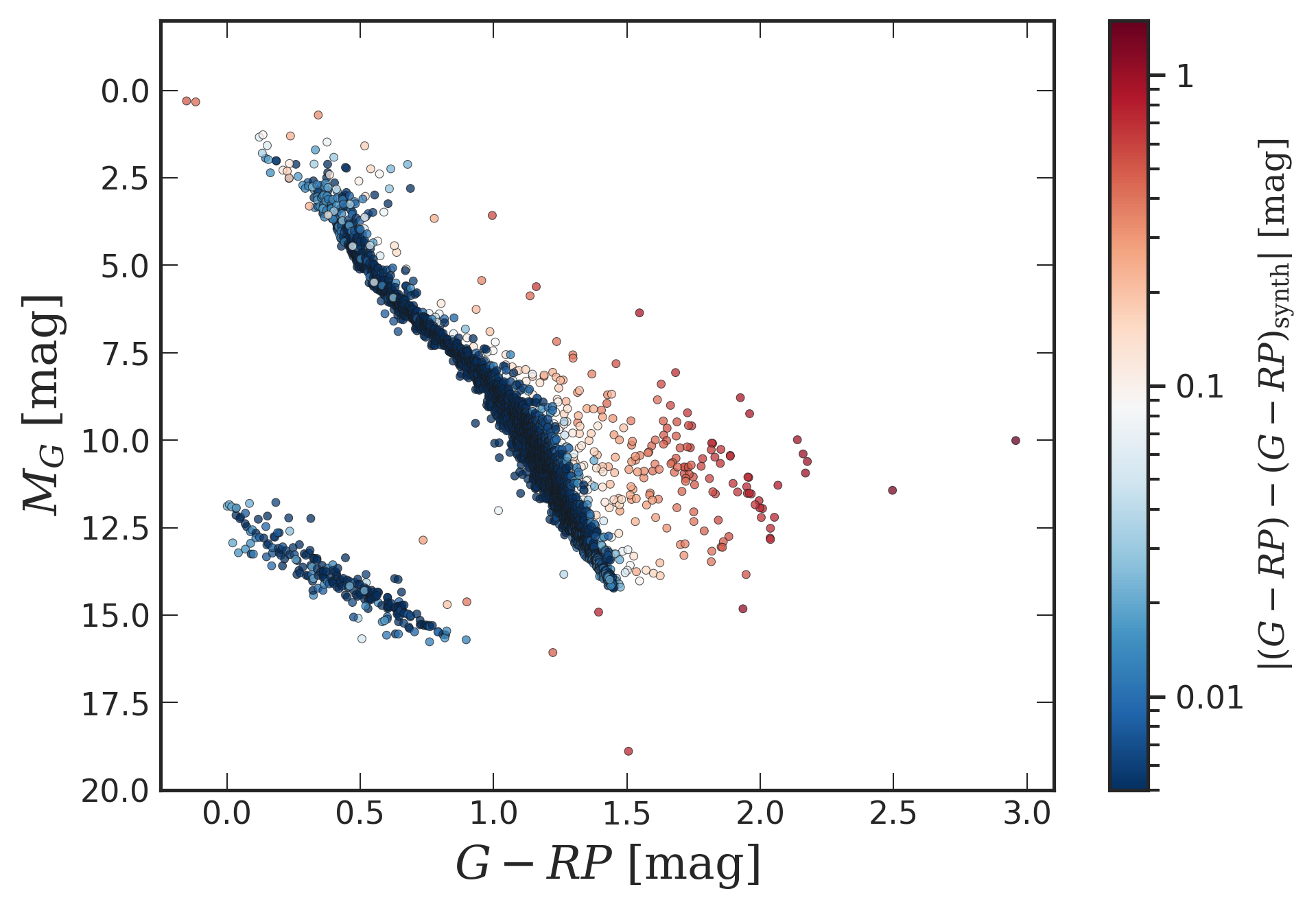
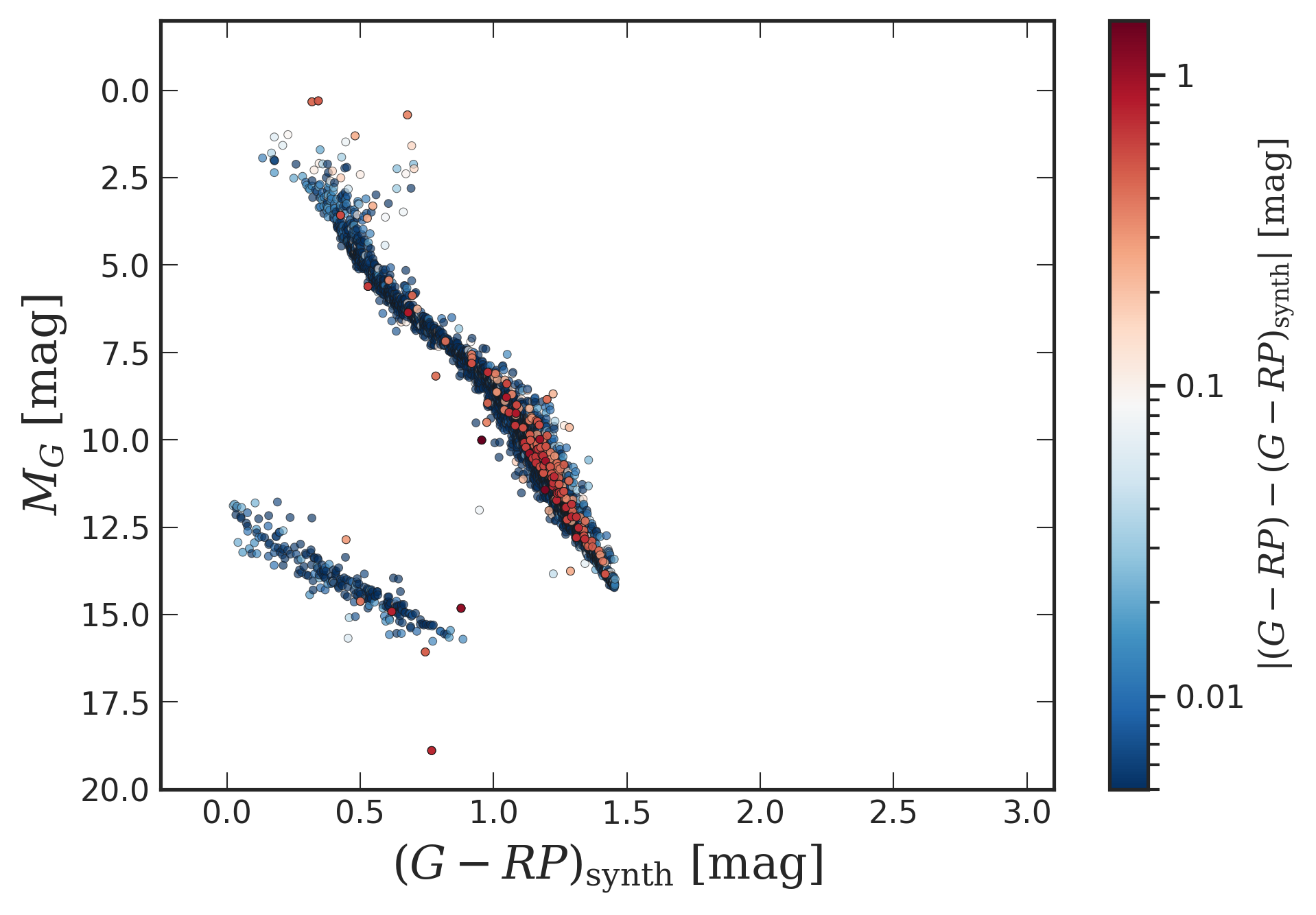
Figure 3: (Top): CMD for objects in the CNS5 which have a counterpart in Gaia EDR3 using the published $G-RP$ colour.
(Bottom): CMD for the same sample, but using synthetic (deblended) $G-RP$ colours. The colour bar shows the absolute difference between the measured and synthetic $G-RP$ colours. The stars coded in red are the ones with the largest differences between the two colours.

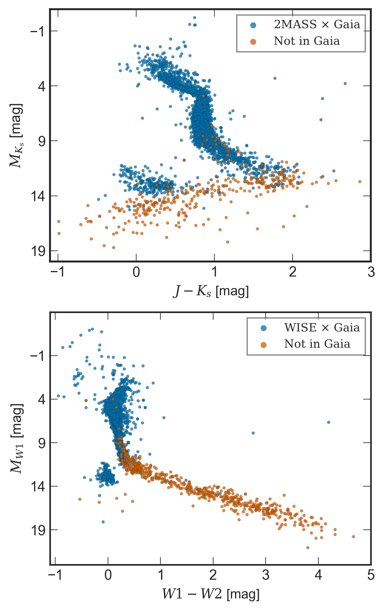
Figure 4: (Top): CMD of the 2MASS sample. The blue points represent 2MASS sources cross-matched with Gaia EDR3 while the orange ones are not present in Gaia. Six extreme outliers are out of this frame.
(Bottom): Similarly, a CMD of the WISE sample, with the blue points representing WISE sources cross-matched with Gaia EDR3 while the orange ones are not present in Gaia. Two extreme outliers are out of this frame.

For objects with photometry in Gaia EDR3 we also list the synthetic (deblended) $G$ and $G-RP$ magnitudes. These are calculated from our model fit to the Gaia data for a sample of objects with high-quality photometry and is fully described in Appendix B. The deblended magnitudes in our catalogue are provided only for sources with a sufficiently large flux-over-error ratio in $BP$ and $RP$ bands ($I_{BP,\,RP}/\sigma_{I_{BP,\,RP}}>20$) and with a colour within the applicability range of $0\leavevmode\nobreak\ {\rm mag}<BP-RP<4.25$ mag. We supply the deblended photometry for all sources which match these criteria, irrespective of whether the correction is significant or not. In case it is available, the deblended photometry is always given as the resulting photometry.

For all objects selected from the Hipparcos catalogue, which have no counterpart in Gaia EDR3, we provide converted values of $G$ and $RP$ magnitudes. Converted magnitudes were calculated using the photometric relationships $G-H_{p}=f(V-I)$ from Riello et al. (2021). We opted for this parameter space because here, contrary to ($G-H_{p},B-V$), red giants and dwarfs display the same behaviour and no distinction between them is needed. However, the reader should be aware that $V-I$ colours in Hipparcos are a compilation from the literature and originate from a variety of ground-based measurements obtained more than 30 years ago. As demonstrated by Koen et al. (2002) and by Platais et al. (2003), $V-I$ colours listed in Hipparcos in some cases can be grossly incorrect and should be treated with caution.

Figure 5: CMD of CNS5 objects in Gaia EDR3 and WISE bands. The main plot includes Gaia EDR3 objects with resulting $G-RP$ colours. This includes objects with synthetic colours and also objects which fall out of its applicability range. It also includes objects from Hipparcos which do not have a counterpart in Gaia EDR3, with converted $G$ and $RP$ magnitudes. The top and right axis show the spectral type and the blue cross represents the Sun’s location on this CMD.The grey shaded area corresponds to the region in which the number of MS objects not present in Gaia start to increase in WISE bands. Thus, this region is also represented as an inset plot in WISE bands with the spectral type on the top axis. The colour bar shows the density in terms of star counts per pixel. On the main plot, each pixel is $[0.020\times 0.15]\leavevmode\nobreak\ {\rm mag}^{2}$ while on the inset plot it is $[0.045\times 0.25]\leavevmode\nobreak\ {\rm mag}^{2}$. One extreme outlier falls outside of the main plot region.

The remaining columns referring to photometry contain NIR and MIR magnitudes in the 2MASS ($J,H$ and $K_{s}$) and WISE ($W1,W2,W3$ and $W4$) passbands with their corresponding uncertainties. We used the cross match between Gaia and 2MASS and Gaia and WISE, respectively, provided with Gaia EDR3 for the identification of objects.

Further, we list the number of components in each system in the CNS5. We made an effort to identify at least obvious common proper motion pairs in the CNS5 by selecting pairs with projected separation less than 1 pc and proper motions consistent with a Keplerian orbit (see El-Badry et al. 2021, Equation 1 and Equations 3–6 in their paper).

The limit on the projected separation of 1 pc corresponds to the separation where the Galactic tidal field typically starts to dominate the gravitational attraction of two stars (e.g. Binney & Tremaine 2008; El-Badry et al. 2021). The chosen limit seems to be appropriate since we found no pairs with a projected separation above 0.85 pc, and only two pairs ($0.3\%$) with a projected separation larger than 0.33 pc. All separations are thus well below the adopted limit, so that these systems have a large probability of being physically associated. The mean projected separation of the identified common proper motion pairs is 1857 AU, whereas the median is 185 AU (corresponding to an orbital period of $\sim 80\,000$ years and $\sim 2500$ years, respectively, for a typical binary with a total mass of $1M_{\sun}$).

We consider a pair of stars to be a common proper motion pair if its observed scalar proper motion difference does not exceed the maximum expected proper motion difference for a circular orbit of a binary with a total mass of $5M_{\sun}$ at the $2\sigma$ level. For $86.6\%$ of the identified pairs, we found that the observed proper motion difference is at least two times smaller than the expected difference due to orbital motion. Only $0.6\%$ (four pairs) have a proper motion difference larger than the expected difference due to orbital motion but still consistent at the $2\sigma$ level with a Keplerian orbit. Loosening this selection criterion further would result in contamination from chance alignments with background stars.

When it comes to identifying common proper motion pairs in the CNS5, we decided to neglect the parallax discrepancy. In this way we can include also those nearby systems whose physical separation between components is large enough that their parallaxes differ significantly. This choice is justified by the low projected source density in the CNS5 catalogue and large parallaxes and proper motions of objects in the solar neighbourhood. We found that parallax discrepancy, $\Delta\varpi/\sigma_{\Delta\varpi}=|\varpi_{1}-\varpi_{2}|/\sqrt{\sigma_{\varpi_{1}}^{2}+\sigma_{\varpi_{2}}^{2}}$, for nearby binaries in Gaia EDR3 could be as large as $11.9\sigma_{\Delta\varpi}$ (Gaia~EDR3~5479222240596469632 and Gaia~EDR3~5287046368477870848).

Finally, we would like to remark that the common proper motion pairs identified in the CNS5, by construction, include all the nearby binaries from El-Badry et al. (2021) as well as systems with three or more components and pairs where only one component has parallax and proper motion given in Gaia EDR3 and the second has them from other surveys, for instance from Spitzer. This results in 696 common proper motion pairs in the CNS5.

So far, we consider for the number of components given in the catalogue only visual binary or multiple components, i.e. those which have a separate entry in the CNS5 catalogue. Spectroscopic companions or otherwise detected companions from the literature will be added in the next version of the CNS catalogue.

Finally, we provide radial velocities from Gaia EDR3 or from the compilations by Best et al. (2021) where available.

Table 2: Description of the CNS5 content. The entry for Proxima Centauri (GJ~551) is shown as an example.

Column name	Unit	Description	Example
cns5_id		CNS5 designation	3591
gj_id		Gliese-Jahreiß number	551
component_id		Suffix for a component of binary or multiple system	C
n_components		Total number of components in the system	3
primary_flag		Flag indicating the primary of a multiple system	False
gj_system_primary		GJ number of the primary component of the system	559
gaia_edr3_id		Source identifier in Gaia EDR3	5853498713190525696
hip_id		Hipparcos identifier	70890
ra	deg	Right ascension	217.39232147200883
dec	deg	Declination	-62.67607511676666
epoch	a	Reference epoch for coordinates	2016.0
coordinates_bibcode		Reference for ra, dec	2020yCat.1350….0G
parallax	mas	Absolute trigonometric parallax	768.0665391873573
parallax_error	mas	Error of parallax	0.056201234
parallax_bibcode		Reference for parallax	2020yCat.1350….0G
pmra	mas a-1	Proper motion in right ascension ($d(\alpha\cos\delta)/dt$)	-3781.741008265163
pmra_error	mas a-1	Error of pmra	0.03138607740402222
pmdec	mas a-1	Proper motion in declination	769.4650146478623
pmdec_error	mas a-1	Error of pmdec	0.05052453279495239
pm_bibcode		Reference for proper motion	2020yCat.1350….0G
rv	km s-1	Radial velocity (spectroscopic)	-22.4
rv_error	km s-1	Error of rv	0.5
rv_bibcode		Reference for the radial velocity	2006A&A…460..695T
g_mag	mag	$G$ band mean magnitude (corrected)	8.984749
g_mag_error	mag	Error of g_mag	0.0007106
bp_mag	mag	Gaia EDR3 integrated $BP$ mean magnitude	11.373116
bp_mag_error	mag	Error of bp_mag	0.0025825
rp_mag	mag	Gaia EDR3 integrated $RP$ mean magnitude	7.5685353
rp_mag_error	mag	Error of rp_mag	0.0017553
g_mag_from_hip	mag	Converted $G$ band magnitude from Hipparcos
g_mag_from_hip_error	mag	Error of g_mag_from_hip
g_rp_from_hip	mag	Converted $G-RP$ colour from Hipparcos
g_rp_from_hip_error	mag	Error of g_rp_from_hip
g_mag_resulting	mag	Resulting $G$ band magnitude	8.984749
g_mag_resulting_error	mag	Error of g_mag_resulting	0.0007106
g_rp_resulting	mag	Resulting $G-RP$ colour	1.3984906
g_rp_resulting_error	mag	Error of g_rp_resulting	0.0033824
g_rp_resulting_flag		Flag related to g_rp_resulting	0
		and g_rp_resulting_error
j_mag	mag	2MASS $J$ band magnitude	5.357
j_mag_error	mag	Error of j_mag	0.023
h_mag	mag	2MASS $H$ band magnitude	4.835
h_mag_error	mag	Error of h_mag	0.057
k_mag	mag	2MASS $K_{s}$ band magnitude	4.384
k_mag_error	mag	Error of k_mag	0.033
jhk_mag_bibcode		Reference for NIR magnitudes	2003tmc..book…..C
w1_mag	mag	WISE $W1$ band magnitude	4.195
w1_mag_error	mag	Error of w1_mag	0.086
w2_mag	mag	WISE $W2$ band magnitude	3.571
w2_mag_error	mag	Error of w2_mag	0.031
w3_mag	mag	WISE $W3$ band magnitude	3.826
w3_mag_error	mag	Error of w3_mag	0.015
w4_mag	mag	WISE $W4$ band magnitude	3.664
w4_mag_error	mag	Error of w4_mag	0.024
wise_mag_bibcode		Reference for MIR magnitudes	2014yCat.2328….0C

Table 3: Description of the photometric content of the CNS5.

Parameter	# of objects
g_mag	5234
bp_mag	5148
rp_mag	5157
g_mag_from_hip	137
g_rp_from_hip	137
g_mag_resulting	5372
g_rp_resulting	5261
j_mag	5348
h_mag	5347
k_mag	5334
w1_mag	4812
w2_mag	4814
w3_mag	4812
w4_mag	877
Has k_mag but no g_mag_resulting	334
Has g_mag_resulting but no k_mag	372
Has w1_mag but no g_mag_resulting	537
Has g_mag_resulting but no w1_mag	1097

4.3 Availability of the CNS5 catalogue

The CNS5 catalogue is hosted by the German Astrophysical Virtual Observatory (GAVO) and is also available through the VizieR Catalogue Service.

5 Catalogue properties

5.1 Colour-magnitude diagrams

Figure 3 (top) shows the CMD for the selection of Gaia EDR3 objects in the CNS5 with published (i.e.  unadjusted) colours. Here, we see that some objects have a large offset towards the red of the main sequence (MS), which is unphysical and is caused by blending or contamination from nearby sources.

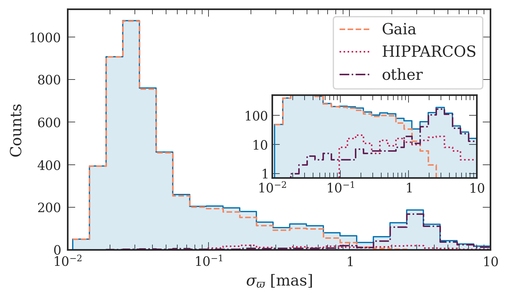
Figure 6: Parallax uncertainties in the CNS5. The inset represents the zoom-up of the vertical axis and with logarithmic scale being used on each of the axes. Distributions of the parallax uncertainties in the subsamples from Gaia, Hipparcos and other references are overplotted separately.

In order to correct for it, we derive synthetic $G-RP$ magnitudes (see Appendix B for details) in the applicability range of $0\leavevmode\nobreak\ {\rm mag}<BP-RP<4.25\leavevmode\nobreak\ {\rm mag}$ and if the flux over error is greater than 20 for both $BP$ and $RP$ magnitudes. Figure 3 (bottom) shows the CMD using these synthetic $G-RP$ magnitudes for all stars, although the corrections are small for many of them (coded in blue in the figure). The stars coded in red colours have large corrections, and they now all fall right on the main-sequence where one would expect them, illustrating that our correction works extremely well.

In Fig. 4 we show the infrared CMDs using 2MASS (top) and WISE (bottom) photometry. In both diagrams the blue points are sources with a counterpart in Gaia EDR3, while the objects in orange are absent in Gaia EDR3. In the 2MASS CMD, the lowest mass objects turn left towards the blue. This effect is associated with the 1.6 and 2.2 µm methane absorption bands (Burgasser et al. 1999) and with the dissipation of clouds across the L/T transition of brown dwarfs (Saumon & Marley 2008). As the absorption in cooler T dwarfs gets stronger, making their $J-K_{s}$ colour bluer, these low-mass brown dwarfs approach the location of the white dwarfs (WDs) in the CMD. In contrast, in WISE $W1-W2$ colour the ultra-cool dwarfs continue the trend towards the red for lower masses. As a result, the lower end of the MS in WISE is well separated from the WDs. Photometric errors for the fainter objects in particular are also smaller in WISE, and as seen in Sect. 4.2, WISE goes deeper and is more complete for ultra cool dwarfs than 2MASS, thus making WISE ideal to study the faint end of the main-sequence.

In Fig. 5, we present the CMD of the CNS5 objects in Gaia EDR3 and WISE bands combined. We use synthetic Gaia colours (Appendix B) where applicable, and have converted the magnitudes and colours of Hipparcos stars into the Gaia system to also include those stars in the plot. There are still a few stars located redwards of the main-sequence; these are all stars for which we could not provide deblended magnitudes, because they fall outside of the colour range where a reliable correction could be derived, or they have S/N smaller than 20. Their colours in the CMD are still dominated by blending or contamination, whereas their $G$ band absolute magnitude is reliable. We note that for objects in our catalogue the uncertainty of position in the CMD is dominated by colour uncertainty and not by that of the parallax. The mode of the underlying parallax error distribution in the CNS5 is $0.025\leavevmode\nobreak\ \text{mas}$ (see Fig. 6). This means that the parallax uncertainty typically contributes only about $0.0014\leavevmode\nobreak\ {\rm mag}$ to the uncertainty of the absolute magnitude for an object at the 25 pc distance, whereas the mode of $G-RP$ uncertainty distribution is $0.0018\leavevmode\nobreak\ {\rm mag}$. From Fig. 4 (bottom) we know that the number of MS objects which do not have a counterpart in Gaia EDR3 starts to increase from $M_{W1}\gtrsim 9\>\leavevmode\nobreak\ {\rm mag}$ or $M_{G}\gtrsim 14\>\leavevmode\nobreak\ {\rm mag}$ (cf. Fig. 9). This region is indicated by the grey shaded area in the main plot. We show this lower-main sequence region as an inset plot in the WISE bands, where completeness is much higher than in Gaia.

5.2 Completeness of the CNS5

A precise assessment of the completeness of the CNS5 catalogue is essential not only to know until which absolute magnitude or spectral type we are complete, but it is also a crucial component for deriving a luminosity function (see Sect. 5.3) and for many other similar applications. Using a number density simply computed for the volume with 25 pc radius would yield a luminosity function which is heavily biased due to incompleteness at the faint end. Consequently, number densities at faint magnitudes would be underestimated. In contrast, when number densities are derived within the completeness limit, this bias is avoided.

Assuming that stars in the solar neighbourhood have a constant number density, we define the completeness limit of the CNS5 as the largest distance $r_{c}$ at which the distribution of objects in the catalogue is still consistent with being spatially uniform. Beyond this distance the observed number density starts to drop because more and more objects are too faint to be observed (or to have reliable parallaxes) and hence are missed in our volume-limited sample. Furthermore, it is natural to expect that the distance $r_{c}$ will be smaller for objects with fainter absolute magnitudes.

A uniform space density prior is reasonable for our 25 pc sample also because there are no known clusters within this distance. The nearest cluster, the Hyades, is located at a distance of $47.50\pm 0.15$ pc of the Sun (Gaia Collaboration et al. 2018), has half-mass radius of 4.1 pc and tidal radius of 9 pc (Röser et al. 2011). Using Gaia DR2, the present-day tidal tails of the Hyades were mapped within 200 pc of the Sun and there are only 18 probable members and 3 contaminants located within 25 pc of the Sun (Röser et al. 2019). According to Jerabkova et al. (2021), the number of candidate members of the Hyades tidal tails located within 25 pc is even lower: they confirm only 7 members using Gaia DR2 and 5 members when using more precise astrometry from Gaia EDR3 in their analysis. These numbers are not large enough to yield any statistically significant overdensity within our 25 pc volume or to contaminate the luminosity function of the solar neighbourhood.

We assessed the completeness of our catalogue using a Kolmogorov-Smirnov test. Here, we select a subsample of stars for each absolute magnitude bin for which a completeness limit should be estimated. Then for each such subsample the cumulative distribution function (CDF) of the distance $r$ is derived and compared with the expected CDF of a uniform distribution. A note should be made here that we do this on the component level and not on the system level. For simplicity, stars with distances close to the 25 pc limit were treated according to their nominal parallax values.

By applying the Kolmogorov-Smirnov test, we find the largest distance $r_{c}$ within 25 pc at which both, the empirical and the uniform CDF, are statistically indistinguishable at the 5% level. Within the derived distance $r_{c}$ our catalogue can be regarded as statistically complete for the probed magnitude interval.

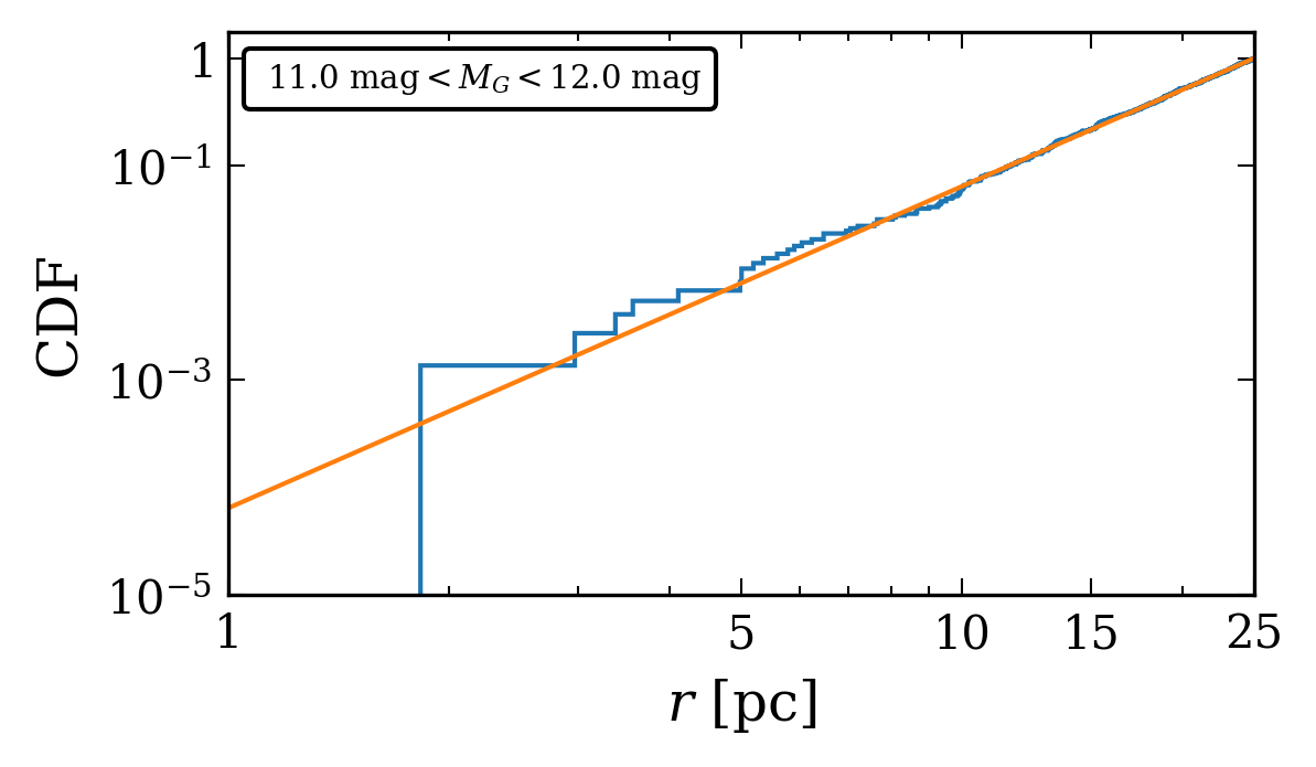
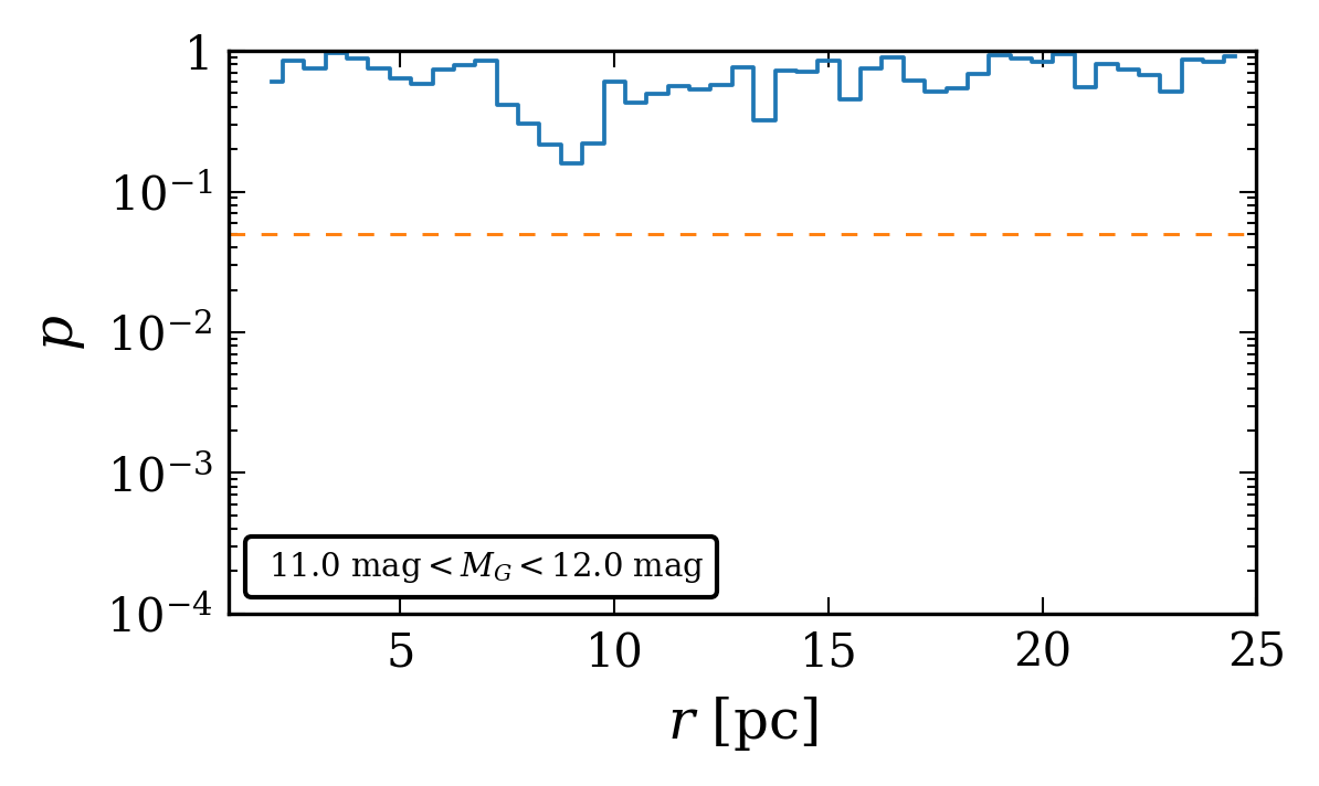
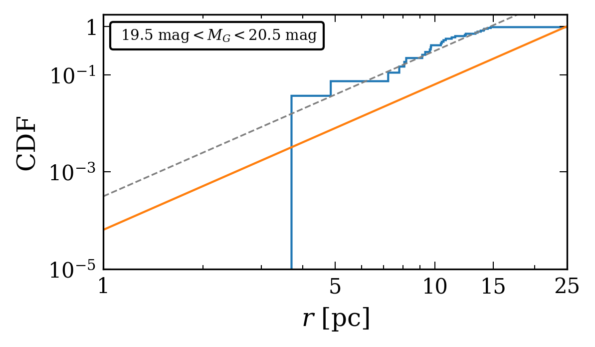
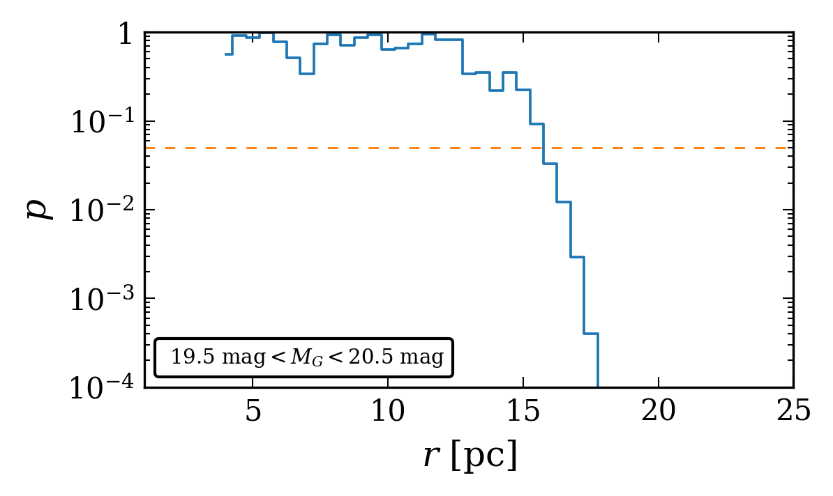
Figure 7: Here we illustrate how we estimate the completeness limit with the help of the Kolmogorov-Smirnov test. The left column shows the empirical (shown in blue) and analytical (shown in orange) CDFs. The right column shows the $p$-value from the Kolmogorov-Smirnov test as a function of probed distance limit. The dashed line indicates the $p=0.05$ threshold. Values below the threshold indicate that the empirical and analytical CDFs are significantly different, which means that the spatial distribution of objects in the subsample is not uniform anymore. Thus, the subsample cannot be regarded as statistically complete beyond the completeness radius. Two magnitude ranges are shown here as an example. The dashed line in the lower left panel denotes the re-normalised CDF using the derived completeness limit for this magnitude bin.

Here we recall that the analytical CDF of the cumulative number of stars as a function of distance $n(r)$ for a sphere of radius $R_{0}=25\leavevmode\nobreak\ {\rm pc}$ and uniform space density can be derived from the normalised probability density function (PDF):

$$n(r)=3\frac{r^{2}}{R_{0}^{3}}.$$ (5)

Thus, the CDF of $n(r)$ is given as:

$$\left.\begin{aligned} CDF(r)=\frac{r^{3}}{R_{0}^{3}},&\qquad{0\leq r\leq R_{0}}.\end{aligned}\right.$$ (6)

For each empirical sample we construct a corresponding test sample of $10^{4}$ objects. The distance of an object in the test sample is given by

$$r=R_{0}\cdot y^{\frac{1}{3}},$$ (7)

where $y$ is a random number between zero and one.

Fig. 7 examplifies CDFs and results of the Kolmogorov-Smirnov test for two cases. While the distribution of the sources in the magnitude bin centered at $G=11.5\leavevmode\nobreak\ {\rm mag}$ (upper row) is consistent with being uniform over all probed distances up to 25 pc, it is evident that the empirical and analytical CDFs of the sources in the bin at $G=20\leavevmode\nobreak\ {\rm mag}$ are considerably different (lower left panel) and the sample is statistically complete only up to 16 pc (lower right panel). For illustrative purposes, we show that the empirical CDF is represented by the analytical CDF quite well when the latter is normalised at the derived completeness limit (dashed line in the lower left panel).

Following the approach outlined above, we derive a completeness limit of 18.9 mag in G-band and of 11.8 mag in W1-band absolute magnitudes (Fig. 8).

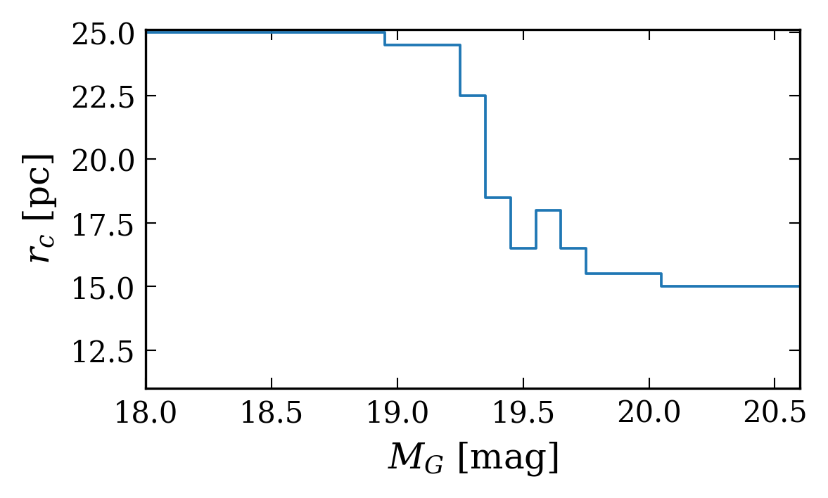
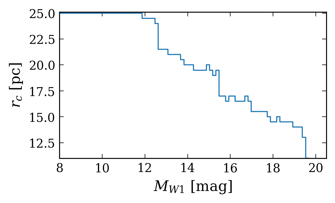
Figure 8: Left: Completeness limit as a function of absolute magnitude in the $G$-band. The limit is computed for a sliding bin with 0.1 mag step and 1 mag bin width. Right: Completeness limit as a function of absolute magnitude in the $W1$-band. Here a 0.15 mag step and a 2 mag bin width was used. The completeness limits are 18.9 mag in G band and 11.8 mag in W1.

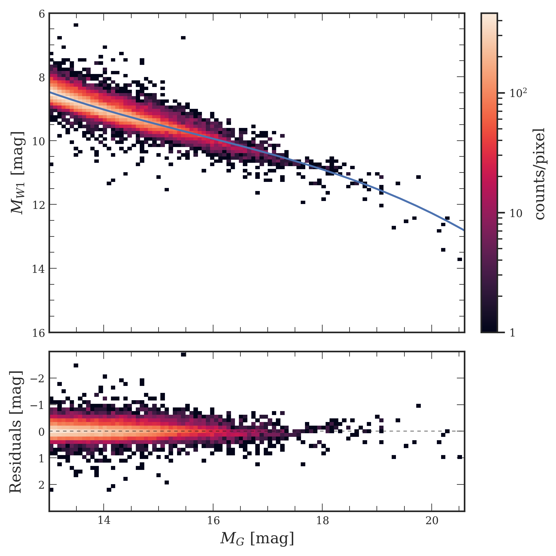
Figure 9: Relation between the absolute magnitude in $G$ and $W1$ bands for the main-sequence stars fainter than $M_{G}=13.0\leavevmode\nobreak\ {\rm mag}$. The solid blue line is the approximate relation in Eq. (9).

When comparing the completeness limits or the luminosity functions in optical and mid-infrared wavelengths, an approximate relation between the absolute magnitudes in these wavelengths is useful. In order to derive the transformation coefficients, we used the sample of the main-sequence stars from the GCNS with counterparts in the CATWISE catalogue (Eisenhardt et al. 2020), in order to make the sample larger but comparable to the CNS5. We used the following criteria:

$$\begin{aligned} \text{(i)}\quad&M_{G}>13.0\leavevmode\nobreak\ {\rm mag},\\ \text{(ii)}\quad&\texttt{gcns\_prob}>0.99,\\ \text{(iii)}\quad&\texttt{wd\_prob}<0.05,\\ \text{(iv)}\quad&\text{Eq.\leavevmode\nobreak\ \eqref{eq:ipd_gof_harm_ampl_cut}:}\ A_{\rm GoF}<10^{-5.12}\leavevmode\nobreak\ (\varpi/\sigma_{\varpi})^{2.61}.\\ \end{aligned}\quad$$ (8)

The resulting sample contains 31 875 sources.

An approximate transformation between $M_{W1}$ and $M_{G}$ magnitudes can be obtained with a cubic polynomial fit in this sample, for which we obtain

$$M_{W1}=0.0073714\,{M_{G}}^{3}-0.3474\,{M_{G}}^{2}+5.896\,M_{G}-25.6\quad,$$ (9)

where all absolute magnitudes are in the unit of mag. The resulting relation for the main-sequence stars fainter than $M_{G}=13.0\leavevmode\nobreak\ {\rm mag}$ is shown in Fig. 9.

Applying this transformation to sources without a counterpart in Gaia EDR3 but with $W1$ magnitudes, so that we obtain approximate $G$ magnitudes for those ultracool dwarfs as well, we estimate that the CNS5 is complete down to $G\approx 19.7\leavevmode\nobreak\ {\rm mag}$ (Fig. 10), 0.8 mag fainter than based on Gaia sources alone.

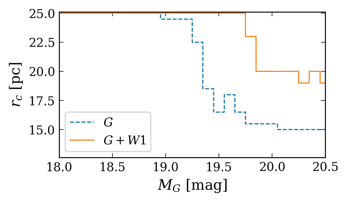
Figure 10: Completeness limit of the CNS5 in $G$-band when ultra-cool dwarfs with converted $M_{G}$ magnitudes are included (solid orange line). The completeness limit in $G$-band from Fig. 8 is shown for comparison (dashed blue line).

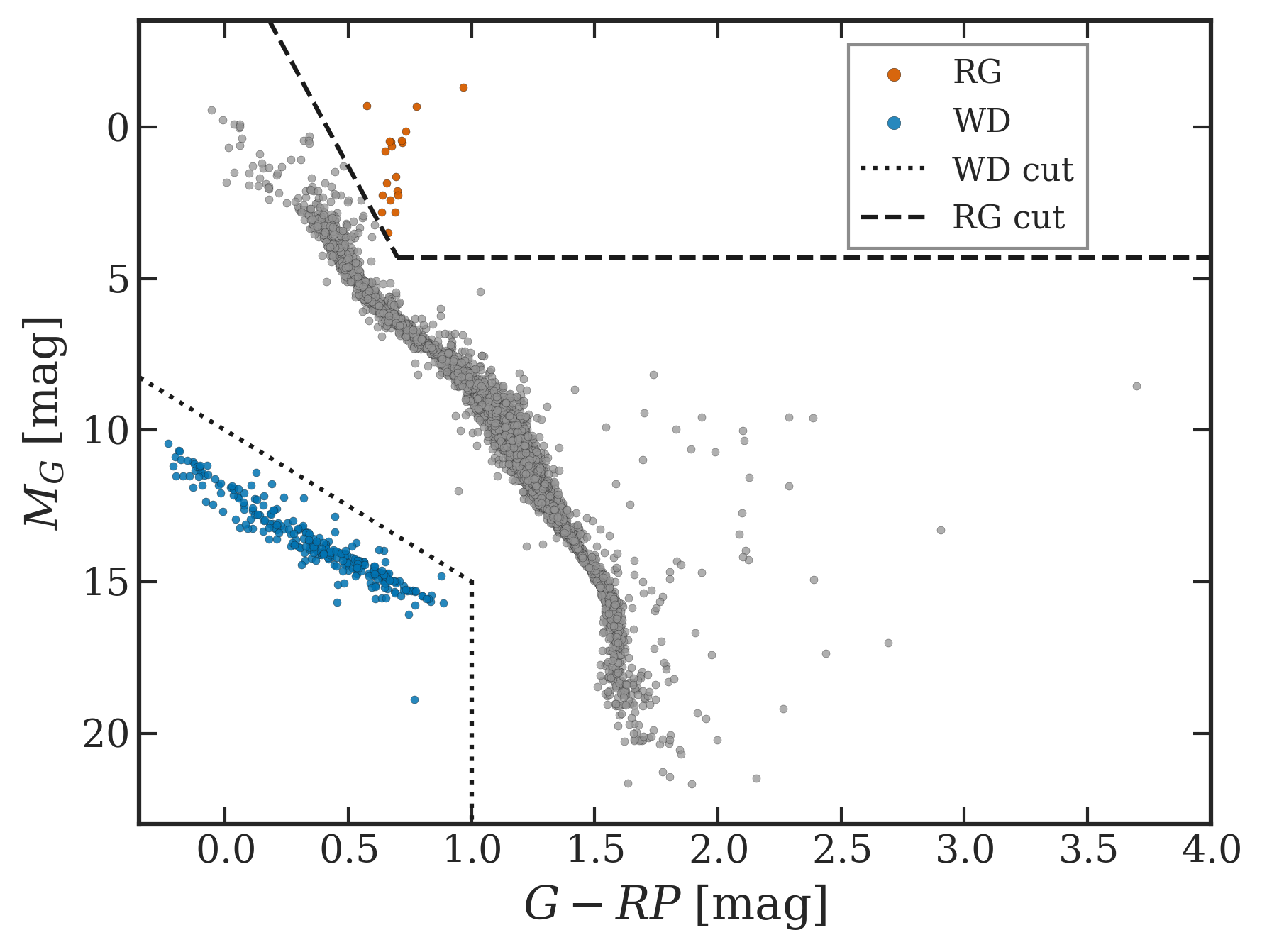
Figure 11: CMD for the Gaia EDR3 and Hipparcos sample in the CNS5. The dashed line separates red giants from the main-sequence stars, while all objects below the dotted line are considered as white dwarfs. We classify the remaining sample as MS stars.

Given that white dwarfs (WD) are quite rare and, as shown later, represent only $5\%$ of the stellar content in the solar neighbourhood, we separately assessed the WD completeness. We selected objects located in the WD region of the CMD by defining the following cut (see Fig. 11):

$$\left.\begin{aligned} \text{(i)}\quad&M_{G}>10.0\leavevmode\nobreak\ {\rm mag}+5(G-RP)\\ \text{(ii)}\quad&G-RP<1.0\leavevmode\nobreak\ {\rm mag}\end{aligned}\quad\right\}$$ (10)

Having applied the Kolmogorov-Smirnov test to the whole WD sample as well as to subsamples of different magnitude bins, we found that the distribution of white dwarfs in the solar neighbourhood is consistent with being uniform and that the 25 pc white dwarf sample can be regarded as statistically complete. Therefore, this eliminates the possible concern that the shape and the location of the cut-off of the observational white dwarf luminosity function are affected by Malmquist bias (e.g. Liebert et al. 1979; Iben & Tutukov 1984; García-Berro & Oswalt 2016). We emphasise that in our completeness assessment we refer to the sample of single or resolved white dwarfs. As for unresolved companions, it plausible to speculate that we are more incomplete, which affects the derived number density of white dwarfs in the solar neighbourhood.

We also assessed the sky distribution of all stars in the CNS5 within the completeness limit and observe that their distribution is not only homogeneous but also isotropic. However, the distribution of ultracool dwarfs in our catalogue with distances beyond the completeness limit has a smaller density in the Galactic plane than outside of it. This indicates that the majority of missing brown dwarfs are probably hiding in the Galactic plane regions. Recently, Best et al. (2021) have performed a detailed analysis of anisotropies of brown dwarfs over the sky. Similarly to what we observe, they concluded that their sample shows a deficiency of brown dwarfs at low Galactic latitudes.

5.3 Luminosity functions

5.3.1 Main-sequence luminosity functions

In this section we illustrate that the CNS5 provides an excellent sample to derive the observational luminosity functions in optical as well as in MIR wavelengths. As a first step, we want to separate our sample into WDs and MS stars. WDs were selected using criteria defined in Eq. (10). The following limit was used to separate red giants (RG) from the main-sequence stars (MS):

$$\left.\begin{aligned} \text{(i)}\quad&M_{G}<-6.2\leavevmode\nobreak\ {\rm mag}+15\,(G-RP)\\ \text{(ii)}\quad&M_{G}<4.3\leavevmode\nobreak\ {\rm mag}\end{aligned}\quad\right\}$$ (11)

As a result of these cuts (see Fig. 11) we get a total of 20 RGs and 264 WDs. All the remaining objects are assumed to belong to the main-sequence.

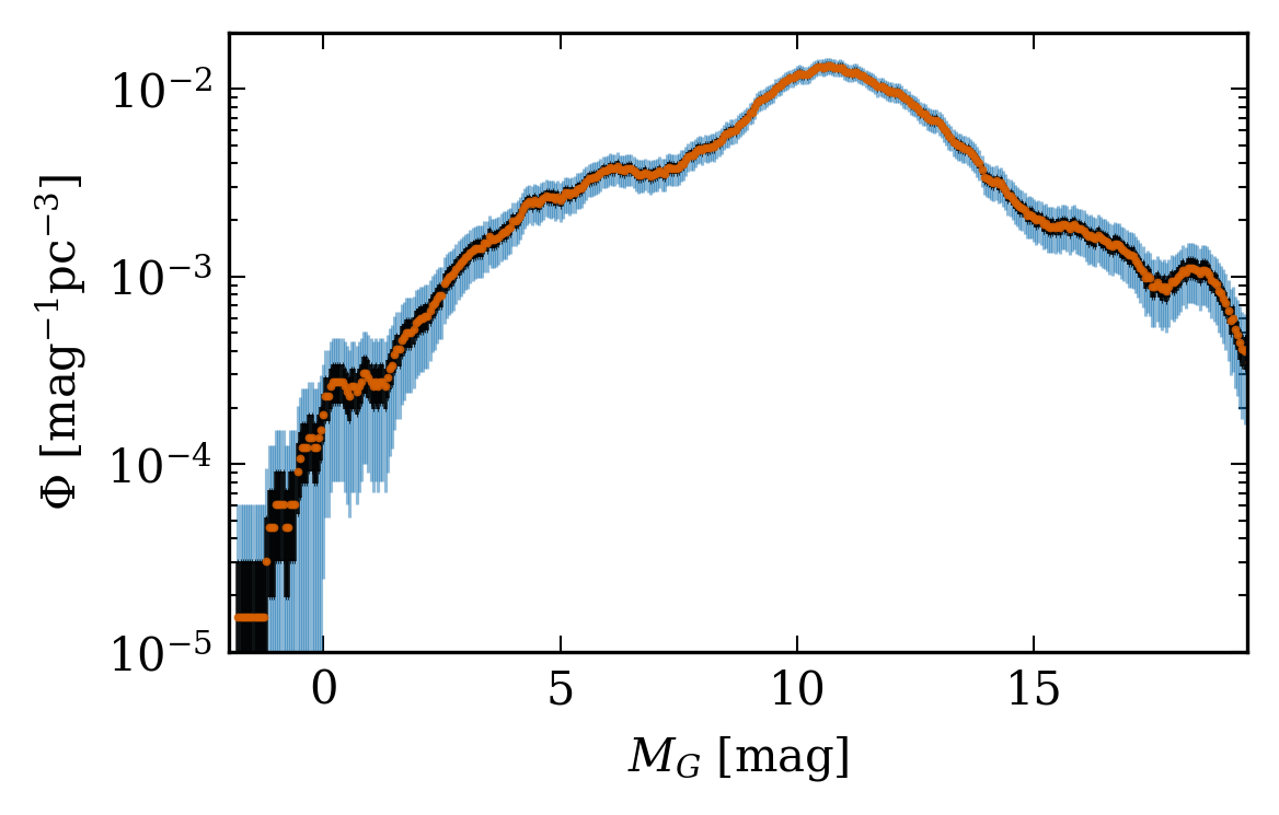
Figure 12: Luminosity function in $G$-band of the main-sequence stars in the solar neighbourhood. Black and blue error bars correspond respectively to $1\sigma\leavevmode\nobreak\ (68.3\%)$ and $3\sigma\leavevmode\nobreak\ (99.7\%)$ confidence intervals.

As it has been demonstrated in the previous section, the CNS5 catalogue is complete down to 19.7 mag in $G$ band. Therefore, the completeness correction was not required there. However, to derive the local observational luminosity function in the mid-infrared, we applied the classical $V_{max}$ technique (Schmidt 1968) using the derived distance limits from a Kolmogorov-Smirnov test to compute the effective limiting volume. The derived luminosity functions for the main-sequence stars are shown in Fig. 12 and 13. It is interesting to note that the presence of the dip at $M_{G}=17.7\leavevmode\nobreak\ {\rm mag}$, where the stellar to substellar boundary is located (Gaia Collaboration et al. 2021b), can be claimed with confidence. Also the increase in the luminosity function after this dip is physical and can be seen in both, optical and MIR luminosity functions.

5.3.2 White dwarf luminosity function

The white dwarf luminosity function (WDLF) is a crucial ingredient for the characterisation of the stellar content of the solar neighbourhood (Weidemann 1967). In particular, the faint end of the WDLF offers the possibility to infer the age of the local stellar population (Schmidt 1959). The finite age of the population and thus limited cooling time of WD progenitors implies that there is an absolute magnitude fainter which no WD can be found in the local population. This is observed as an abrupt cut-off in the WDLF whose position is determined by age of the oldest white dwarfs in the solar neighbourhood (Liebert et al. 1979, 1988; Yuan 1992; Harris et al. 2006; Catalán et al. 2008).

Furthermore, the WDLF is sensitive to the star formation rate (SFR). Thus, inverting the observational WDLF allows to reveal the star formation history of the solar neighbourhood and even to probe star formation bursts occurred in the past (Yuan 1992; Rowell 2013).

However, estimates of both, the SFR as a function of look-back time and of the age of the local population, are dependent not only on the adopted white dwarf evolutionary models, but also sensitive to the properties of the observational dataset which is used to derive the WDLF. Therefore, the observational WDLF will better correspond to reality when derived from a volume-limited sample with maximised completeness and where the absolute magnitudes are estimated using parallaxes with exquisite precision and accuracy and not from reduced proper motions as it was done in the past (e.g. Harris et al. 2006).

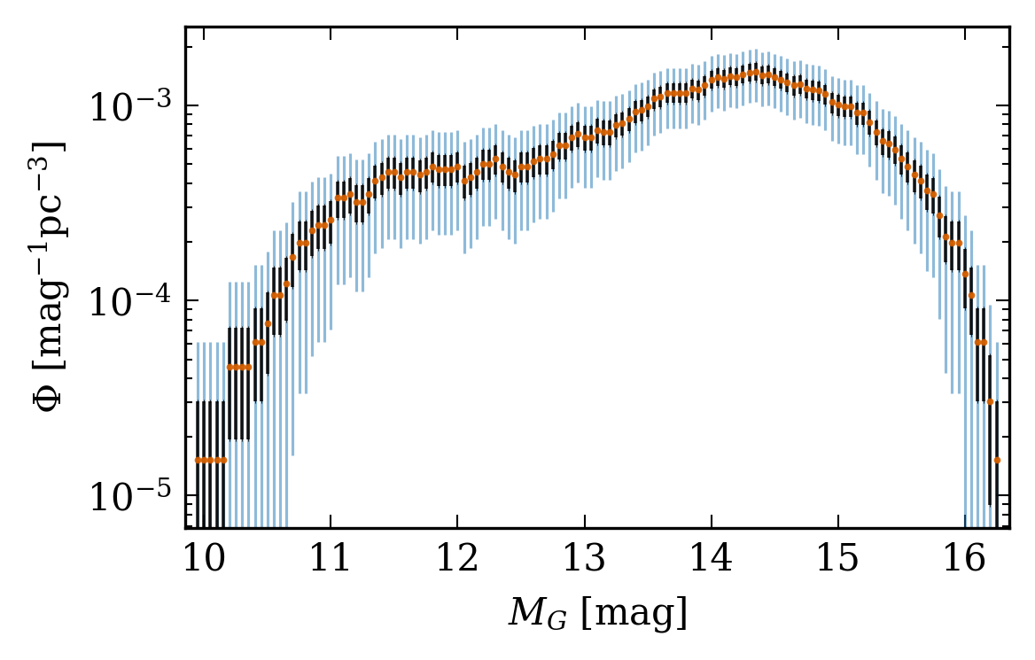
Figure 14: Luminosity function of the white dwarfs in the solar neighbourhood. Black and blue error bars correspond respectively to $1\sigma\leavevmode\nobreak\ (68.3\%)$ and $3\sigma\leavevmode\nobreak\ (99.7\%)$ confidence intervals.

Such a sample of white dwarfs is provided by the CNS5. Thus, we derive the observational WDLF in Gaia’s $G$-band using the same approach as outlined above for MS stars. The derived luminosity function is shown on Fig. 14.

The total number density is another important parameter for describing a local WD population and is also used for the normalisation of the theoretical WDLFs. The CNS5 contains 264 WDs within the 25 pc volume. This translates into a total number density of $(4.03\pm 0.25)\times 10^{-3}\,\text{stars pc}^{-3}$. Our result is consistent with previous findings (Liebert et al. 2005; Gaia Collaboration et al. 2021b).

6 Discussion and Outlook

We first assess the overall completeness of CNS5 based on the completeness limits derived in Sect. 5.2. From Fig. 10, we estimate that we statistically include all systems in the 25 pc volume with absolute $G$ magnitudes brighter than about 19.7 mag (or absolute $W1$ magnitudes brighter than 11.8 mag), corresponding to a spectral type of about L8 (Dupuy & Liu 2012; Pecaut & Mamajek 2013 ). Thus, the CNS5 includes virtually all main-sequence stars as well as virtually all brown dwarfs up to spectral type L8. We stress that our completeness assessment refers to well-resolved components in case of binary or multiple stars; we are certainly more incomplete when it comes to the identification of companions, especially those of low mass or of close separation.

Since we derived the completeness limit in a statistical sense, namely by judging from the density of objects in smaller and closer volumes to larger and more distant volumes, we do not claim that every single system is indeed listed, but the number of missing systems should be rather small compared to the number of objects listed in the catalogue.

This is a major step forward; previous completeness limits for brown dwarfs in particular, but also for M dwarfs, were much closer than the 25 pc distance. The larger volume and larger number of objects that comes with an increased completeness radius enables statistical studies with much smaller error bars.

Previously, RECONS (Henry et al. 2016) had listed 366 objects within the 10 pc sample, which they estimated was 90% complete. CNS5 has added 26 objects within the 10 pc volume, which now contains 392 objects with parallaxes larger or equal to 100 mas. Even when compared to the GCNS and considering the $3\sigma$ confidence interval of the parallaxes, the CNS5 lists 108 more objects within the 10 pc and 739 more within the 25 pc volume because it includes not only Gaia data, but also Hipparcos for the bright stars otherwise missing in Gaia as well as the infrared ground-based parallax survey from Best et al. (2021); Kirkpatrick et al. (2021), which helps tremendously with the completeness of substellar objects.

When comparing the CNS5 with the 10 pc sample from Reylé et al. (2021), we found that the CNS5 adds only two objects not listed in the 10 pc sample, presumably due to the different selection approaches used. Conversely, 148 sources from their 10 pc sample are missing in the CNS5 because they are either an exoplanet, a component of an unresolved binary (these will be part of the CNS6), or if they have a parallax uncertainty $\sigma_{\varpi}>10$ mas or if their parallax was just an estimate without uncertainty (such as CWISE J061741.79+194512.8 AB).

The CNS5 contains 5931 objects in total. Among them, there are 5230 stars (including the Sun, 20 giant stars and 264 white dwarfs) and 701 brown dwarfs. Here, we assume that the approximate stellar/substellar boundary lies at $80\leavevmode\nobreak\ M_{Jup}=0.076\leavevmode\nobreak\ M_{\sun}$, corresponding to spectral type L1 ($M_{G}=16.90\leavevmode\nobreak\ {\rm mag}$ or $W1-W2=0.28\leavevmode\nobreak\ {\rm mag}$). This yields a stellar number density of $(7.99\pm 0.11)\times 10^{-2}\,\text{stars pc}^{-3}$, while the number density for brown dwarfs is $(1.07\pm 0.04)\times 10^{-2}\,\text{objects pc}^{-3}$.

About 72% of stars (or $\sim 63\%$ of stars and brown dwarfs) in the CNS5 are M dwarfs (there are 3760 main-sequence stars in the CNS5 with absolute magnitudes in the range $8.16\leavevmode\nobreak\ {\rm mag}\leq\leavevmode\nobreak\ M_{G}\leq 16.60\leavevmode\nobreak\ {\rm mag}$ as appropriate for M dwarfs, out of a total of 5230 stars). For comparison, the fraction of M-dwarfs in the 10 pc sample was found to be $\sim 61\%$ (Reylé et al. 2021). The number of M-dwarfs within the 25 pc volume could still change in the future, in particular due to unresolved multiple systems in the CNS5.

An interesting quantity is also the fraction of stars relative to the fraction of brown dwarfs, which is directly related to the star formation process. Previous estimates included a factor of 6 times more stars than brown dwarfs in the 8 pc volume by Kirkpatrick et al. (2012), 10 times more stars than brown dwarfs in the 10 pc volume from the RECONS project Henry et al. (2016) and a factor of 5.2 from Bihain & Scholz (2016) within 6.5 pc, while newer estimates seem to converge at a factor around 6–7 Kirkpatrick et al. (2019); Henry et al. (2019). There are 4.4 stars per each brown dwarf listed in the 10 pc sample from Reylé et al. (2021). In the CNS5, the fraction of stars to brown dwarfs is $4.6\pm 0.4$ for the 15 pc volume and it is consistent with the values derived for smaller volumes (see Table 4). Within the total volume of 25 pc, the factor is $7.5\pm 0.3$, indicating that more brown dwarfs than stars are missing at larger distances.

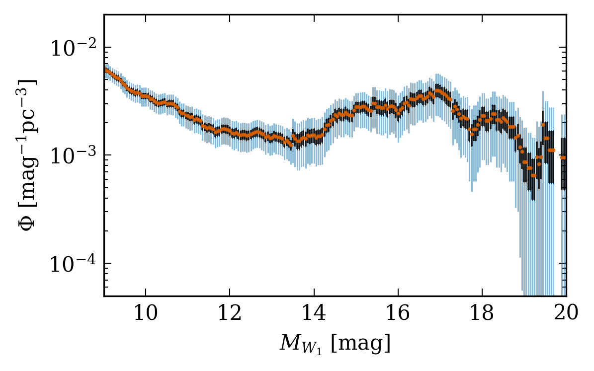
Figure 13: MIR luminosity function of the faint end of the main-sequence. Black and blue error bars correspond respectively to $1\sigma\leavevmode\nobreak\ (68.3\%)$ and $3\sigma\leavevmode\nobreak\ (99.7\%)$ confidence intervals. The shown magnitude range corresponds to the range where the majority of objects with no counterpart in Gaia EDR3 are located (see Fig. 4). $M_{W_{1}}=9\leavevmode\nobreak\ {\rm mag}$ translates approximately to $M_{G}=14\leavevmode\nobreak\ {\rm mag}$.

Table 4: Star to brown dwarf ratio in the CNS5 for different distance limits. The ratio increases significantly at distances larger than 15 pc, indicating that more brown dwarfs than stars are missing at larger distances.

$r$	# of stars	# of BDs	Total	Stars/BDs
6.5 pc	116	22	138	$5.3\pm 1.4$
8.0 pc	164	40	204	$4.1\pm 0.8$
10 pc	319	74	393	$4.3\pm 0.6$
15 pc	1066	231	1297	$4.6\pm 0.4$
20 pc	2590	413	3003	$6.3\pm 0.3$
25 pc	5230	701	5931	$7.5\pm 0.3$

The brown dwarf census is still somewhat limited. Assuming the star to brown dwarf ratio is about 5, we can estimate an approximate number of brown dwarfs currently missing. Knowing that there are 5230 stars in the 25 pc volume, one would expect 1046 brown dwarfs in the same volume. As mentioned above, 701 of them are listed in the CNS5, so that about 345 brown dwarfs are missing. Therefore, we conclude that about one third of brown dwarfs, corresponding to about 6% of all objects within 25 pc, are still to be discovered.

In Sect. 5.2, we have shown that the white dwarf sample in the CNS5 is statistically complete within 25 pc. We derive a number density of white dwarfs of $(4.03\pm 0.25)\times 10^{-3}\,\text{stars pc}^{-3}$. Thus, white dwarfs represent 5% of the local stellar population. We do not see a single faint blue white dwarf as seen by Scholz (2022), but there are only 59 such objects in the GCNS, so our volume of 25 pc might be too small to include one of these rare objects.

Similarly, we do not clearly see the Jao gap (Jao et al. 2018) at absolute $G$ magnitudes of 10.14 mag, although one could notice a small feature if looking closely. The gap becomes more prominent only if looking at larger volumes; it is visible in the GCNS (Gaia Collaboration et al. 2021b).

We plan to compile another version of the CNS, termed CNS6, based on Gaia DR3 in the future. In particular, we will include more information on multiplicity, including spectroscopic companions from the literature and homogeneously derived stellar parameters for all objects in the catalogue.

The CNS5 catalogue also provides the opportunity to investigate the exoplanet inventory in a sample which is unbiased with regard to spectral type or apparent magnitude, in contrast to other typical planet search samples. The planet population within 25 pc might be more representative of the overall planet population in the Milky Way, at least in those environments that resemble the solar neighbourhood, than just the overall known planet population which is highly biased by the sensitivities of the various planet search methods. Furthermore, the astrometric method is most sensitive around the most nearby stars and thus ideally complements our knowledge about exoplanets in the nearby stars sample, which so far mainly comes from the transit and the radial velocity methods. Since astrometry is most sensitive at intermediate periods or semi-major axes, it ideally complements the transit and radial velocity methods which are most sensitive to the shortest periods, and direct imaging detections at the widest separations. Significant contributions regarding intermediate period/semi-major axis planets in the nearby stars sample are expected especially from Gaia DR4, which will also contain epoch astrometry.

Appendix A Selecting astrometrically clean datasets from Gaia EDR3

Data selection from Gaia EDR3 is compromised by the presence of sources with spurious astrometric solutions in the published catalogue. In this section, we discuss our quality cut which eliminates these sources. The validation of this approach will follow in the next subsection.

There is no unique selection criterion (or combination of criteria) which would differentiate between sources with spurious and reliable astrometric solutions in Gaia EDR3 for every use case. For each specific task one should choose individually appropriate selection criteria. Our aim is to define a cut which is conservative enough to retrieve only objects with reliable astrometry (parallaxes in particular). At the same time, the adopted cut should not lessen the completeness of our sample by removing objects which do have reliable parallaxes but with inconsistencies in photometry or even with null values of $G,BP$ or $RP$ fluxes.

$RUWE$ (re-normalised unit weight error; Lindegren 2018) and photometric excess factor (Evans et al. 2018; Lindegren et al. 2018; phot_bp_rp_excess_factor in the Gaia EDR3 catalogue) are the two most widely used parameters in various selection criteria. Deriving both of these parameters involves photometric measurements: the re-normalisation factor of $RUWE$ depends on the magnitude and colour of the source, and photometric excess is defined as the flux ratio $(I_{BP}+I_{RP})/I_{G}$. A deviation from the expected flux excess indicates inconsistency between $G$, $BP$ and $RP$ photometry and therefore often used to exclude such sources. However, one should keep in mind that this metric does not reveal the origin of the inconsistency: it is not possible to distinguish between objects where only $BP$ and $RP$ fluxes from the Gaia photometric instrument are affected and objects where the $G$ flux from the astrometric field is problematic too.

It was shown that both parameters can reach high values for sources with peculiarities in their photometry: an excess in $RUWE$ can be induced by photometric variability or by the presence of an unresolved companion (Belokurov et al. 2020), while the photometric excess factor tends to be larger for objects with peculiar SEDs as well as for various types of variable stars (Riello et al. 2021). Therefore, making the decision whether to include an object in the catalogue or not based on photometric excess or $RUWE$ would bias our catalogue against such types of objects.

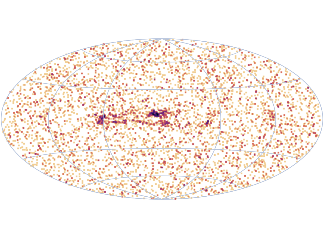
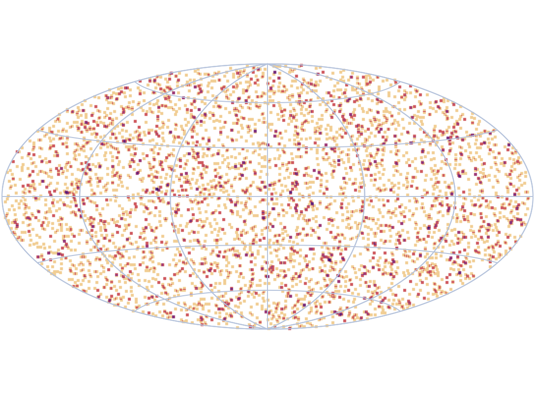
Figure 15: Top: Map of the 25 pc dataset from Gaia EDR3 in Galactic coordinates with $l=b=0$ at the centre. The overdensity along the Galactic plane is an artefact from spurious solutions. Bottom: sources from the 25 pc dataset which remained after applying the cut defined in Eq. (14).

We recall that spurious solutions are often caused by mistakes in cross-matching of individual measurements when assigning the source_id. Measurements of two (or more) different objects associated to the same source_id will result in a spurious catalogue entry: the pipeline interprets the measured displacement as an apparent motion of the object and describes it through a non-physical astrometric solution. This leads to a spuriously large parallax, yet with relatively large formal uncertainties (as a consequence of large centroid dispersion). Obviously, such confusion occurs mostly in crowded fields, for instance, close to the Galactic plane and the Magellanic clouds. This is illustrated by Fig. 15 (top panel): an overdensity along the Galactic plane is clearly visible in the sky distribution of the sample (hereafter, 25 pc sample), retrieved by selecting all objects from Gaia EDR3 satisfying Eq. (1). Furthermore, the mismatching probability for a source also depends on the distribution of scan directions relative to the position angle of confused objects. The necessary information can be obtained from the Image Parameter Determination goodness-of-fit (IPD GoF; Hambly et al. 2021), which is parameterised as

$$\ln(\mathrm{GoF})=c_{0}+c_{2}\cos(2\psi)+s_{2}\sin(2\psi),$$ (12)

where $\psi$ is the position angle of the scan direction and $c_{0},c_{2},s_{2}$ are Fourier coefficients. If an object is a binary, this will be indicated by a large amplitude of the IPD GoF (ipd_gof_harmonic_amplitude in Gaia EDR3), which indicates the level of asymmetry in the image and is computed as

$$A_{\rm GoF}=\sqrt{c_{2}^{2}+s_{2}^{2}}.$$ (13)

Given the above, we can expect a dichotomy between spurious and reliable astrometric solutions in the ($A_{\rm GoF}$, $\varpi/\sigma_{\varpi}$) parameter space. This dichotomy is shown for the 50 pc sample in Fig. 16: sources with spurious solutions (the cluster of points in the top left corner) are well separated from the sources with reliable astrometric solutions.

For an astrometric solution to be considered reliable, we require the source to satisfy Eq. (2), reproduced here for convenience:

$$A_{\rm GoF}<10^{-5.12}\leavevmode\nobreak\ (\varpi/\sigma_{\varpi})^{2.61},$$ (14)

where $\varpi/\sigma_{\varpi}$ corresponds to parallax_over_error as published in the Gaia EDR3 catalogue; that is, parallax zero-point corrections or error inflation are not taken into account for this selection. Here, the slope of the line is chosen so that it follows beneath the cluster of sources with spurious solutions.

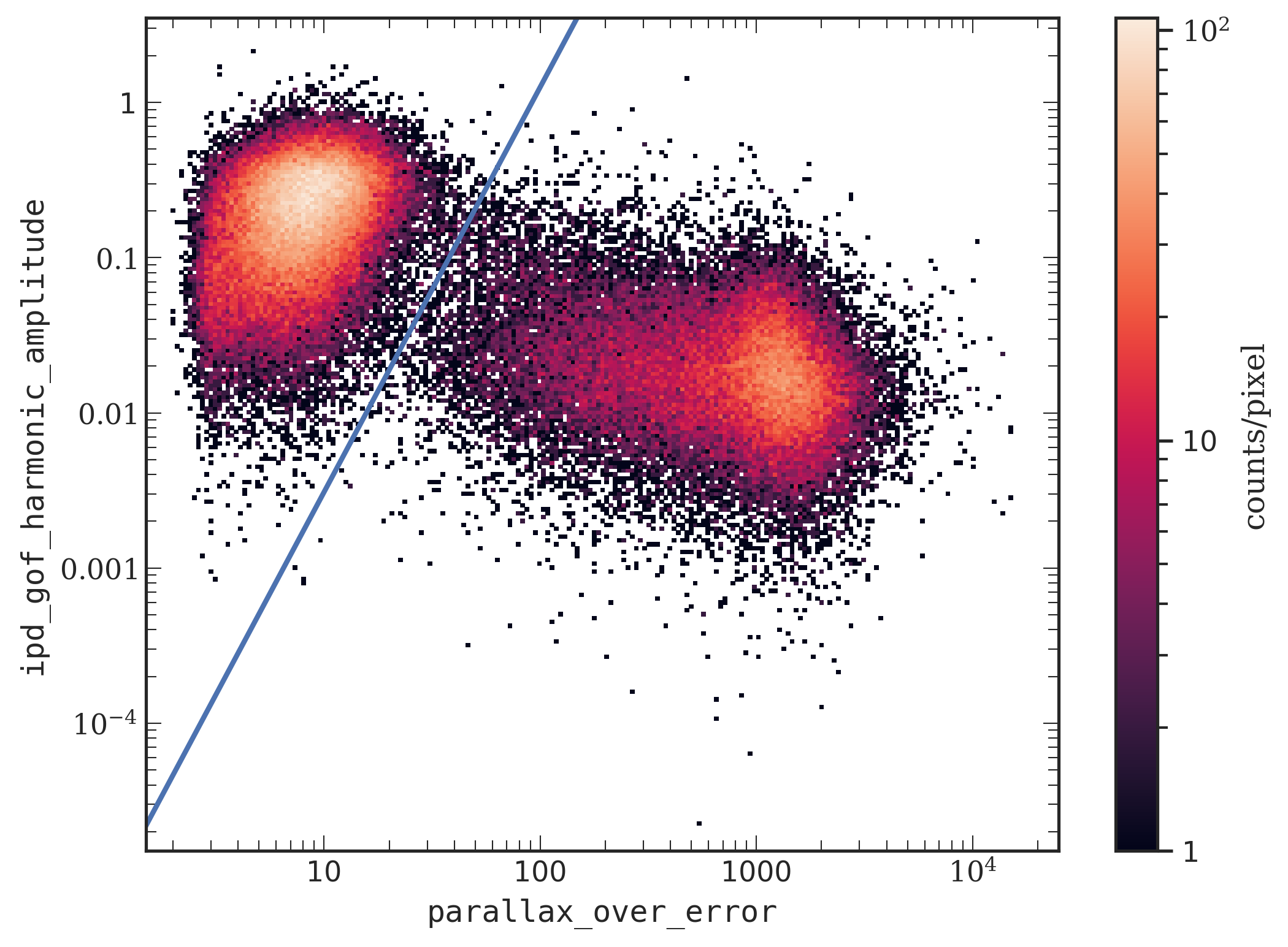
Figure 16: Same as Fig. 1 but for 50 pc sample. As opposed to 25 pc sample, the 50 pc sample is dominated by sources with spurious astrometric solutions: 42 607 sources (50.84%) are located above the blue line – the threshold defined in Eq. (14).

However, this approach comes with its limitation: it works best for nearby stars and it is only applicable in the high-S/N regime. In other words, the cut is tailored to objects with significant parallaxes, where $\varpi/\sigma_{\varpi}$ is larger than that of sources with spurious astrometric solution. For more distant sources (Fig. 16, cf. Fig. 1), the parallax-over-error ratio decreases, the valley between the clusters of spurious and reliable solutions becomes less clean, and the slope of the cut has to be adjusted in each individual case according to demands for completeness and purity.

Figure 17 illustrates that the widely used cut $RUWE<1.4$ is not an optimal approach when completeness of a sample is important. A large number of objects, especially at magnitudes around $G\approx 12\leavevmode\nobreak\ {\rm mag}$, have small amplitudes of the IPD GoF (below the threshold defined by Eq. (14)), but would otherwise have been removed by the cut on $RUWE$. On the other hand, we should note the presence of spurious objects with $G\approx 20\leavevmode\nobreak\ {\rm mag}$ with $RUWE<1.4$. Including them in the sample would contaminate CNS5 and yield an overestimated completeness and distorted luminosity function.

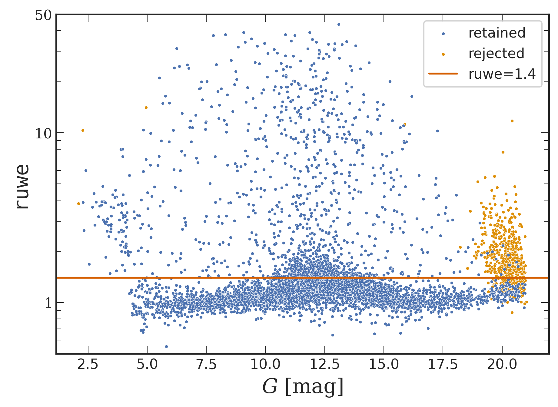
Figure 17: Distribution of $RUWE$ for sources retained (shown in blue) and rejected (shown in yellow) by criterion defined in Eq. (14) as a function of $G$ magnitude. The solid horizontal line shows the $RUWE=1.4$ threshold. Note the presence of rejected sources with $RUWE$ bellow the threshold.

A.1 Selection criterion validation

In the following, we examine whether ipd_gof_harmonic_amplitude and parallax_over_error are sufficient to define a rigorous selection criterion for objects with significant parallaxes to eliminate spurious astrometric solutions in Gaia EDR3 and whether such selection criterion yields results as good as with other classifiers which are in use.

A.1.1 ‘Fidelity’ from Rybizki et al. (2022)

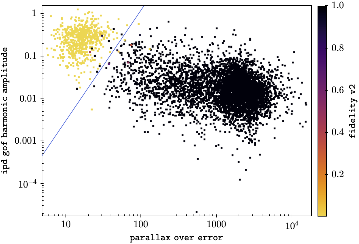
Figure 18: ‘Astrometric fidelity’ from Rybizki et al. (2022) as a function of position in ($A_{GoF},\varpi/\sigma_{\varpi}$) space for all the sources from Gaia EDR3 that are possibly located within 25 pc of the Sun. The blue solid line corresponds to the cut described by Eq. (14).

Rybizki et al. (2022) used machine learning to classify astrometric solutions in Gaia EDR3 and to eliminate spurious solutions. They trained a neural network using 17 parameters from Gaia EDR3 (including ipd_gof_harmonic_amplitude and parallax_over_error) and provided an ‘astrometric fidelity’ for each source - a parameter having values in the range between 0 (spurious solution) and 1 (reliable solution). This approach is somewhat similar to what has been done for the GCNS, now extended to the entire data release.

Here, we validate our cut on harmonic amplitude against the updated version of the classifier (fidelity_v2 column in the gedr3spur.main table). The principal difference between the original (v1) and the updated (v2) classifier is the new high-density training data and crossmatching of the training sample to Pan-STARRS1 instead of to 2MASS in order to avoid bias against faint blue objects (Rybizki et al. 2022).

Figure 18 illustrates the remarkable agreement between our cut and the fidelity parameter. Of the 5184 objects classified as good by us, only 8 have fidelity ¡ 0.9, while there are only 9 sources with fidelity ¿ 0.9 rejected by our cut. Hence we conclude that in $99.84\%$ of the cases the cut on harmonic amplitude and the neural network classifier agree on whether the astrometric solution of an object is spurious or not.

Table 5: Sources in the GCNS within 25 pc rejected by our selection criterion defined in Eq. (14).

Gaia EDR3	Known	$\varpi$	$\sigma_{\varpi}$	$G$	2MASS designation	$K$	$\sigma_{K}$
source_id	binary	[mas]	[mas]	[mag]		[mag]	[mag]
2361294885296927488	N	38.05	1.58	20.80	00135779-2235200	14.04	0.05
4993479684438433792	Y	39.92	0.73	2.09	00261699-4218216	-0.17	0.38
2800081221135505536	N	42.89	1.65	20.83	00282091+2249050	13.78	0.06
5151358868307074432	Y	49.35	1.63	20.23	02052940-1159296	13.00	0.03
251476382498509952	N	36.20	1.74	20.84	03454743+5137159	13.79	0.06
3056233482992410496	N	43.35	1.52	19.69	07414279-0506464	12.39	0.03
761918578311083264	Y	42.24	1.06	19.98	11122567+3548131	12.72	0.03
3591011474602344320	N	43.65	1.99	20.86	11181292-0856106	14.18	0.08
3896357089270247168	N	37.32	2.66	20.70	11582077+0435014	14.44	0.06
1222646935698492160	Y	42.24	0.98	2.27	15344125+2642529	2.21	0.36
5952826016600852352	N	36.13	1.29	20.49	17224991-4449366	¿13.81
2411855072801158656	Y	39.40	1.06	4.95	23190668-1327310	3.35	0.26

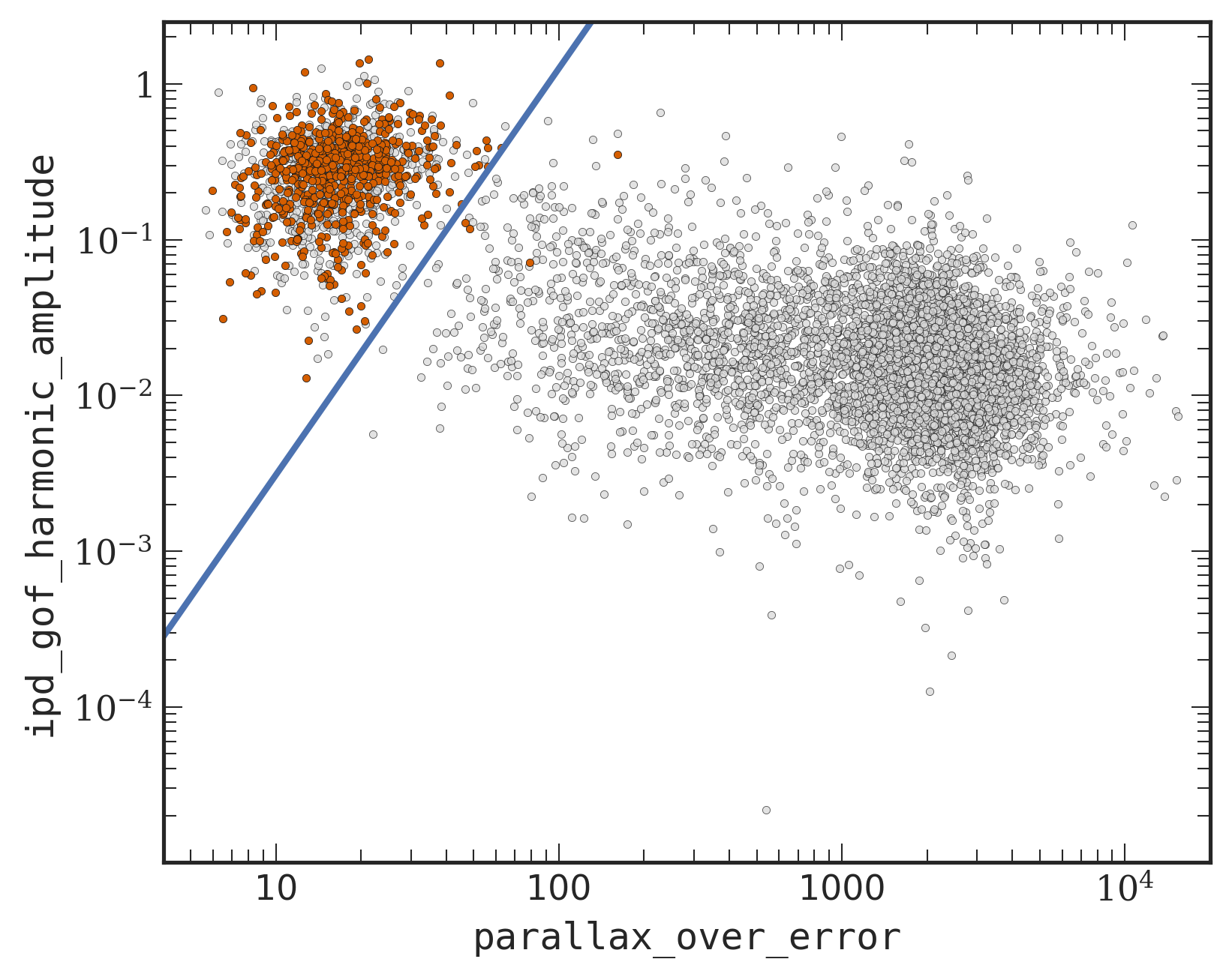
Figure 19: Amplitude of the IPD GoF for the control sample of sources with spurious astrometric solutions as a function of $|\varpi/\sigma_{\varpi}|$ (red markers) overplotted on the 25 pc sample (grey markers). The blue solid line corresponds to the cut described by Eq. (14).

A.1.2 Sample with negative parallaxes

Performance of a selection criterion for a particular sample can be assessed through a control sample of sources with spurious astrometric solutions. Such control sample can be constructed under the fundamental assumption that the probability of positive or negative parallax in a spurious solution is approximately equal; that is, the probability density function is symmetric around $\varpi=0$. Assuming this symmetry and the fact that any astrometric solution with a highly negative parallax (i.e. a negative parallax where the deviation from zero is statistically significant) is spurious by definition, we can estimate the number of sources with spurious solutions in our sample of objects with positive parallaxes (Fabricius et al. 2021). Additional support for this approach comes from Gaia Collaboration et al. (2021b): using the large negative parallax sample, they have constructed the training set for a random forest classifier and utilised it to generate the GCNS.

That being said, we select the control sample symmetrically to Eq. (1):

$$\varpi-3\sigma_{\varpi}\leq-40\leavevmode\nobreak\ \text{mas}.$$ (15)

The resulting sample contains 630 objects.

Consequently, when we apply our cut on harmonic amplitude (Eq. (14)) to the control sample we may infer the fraction of sources with spurious solutions, which are not filtered out by the cut and evaluate whether this fraction is statistically significant. If the cut was perfect it would reject all the objects from the control sample.

In Fig. 19 we show the control sample of sources with spurious solutions in the (ipd_gof_harmonic_amplitude, $|\varpi/\sigma_{\varpi}|$) parameter space (red markers), whilst the 25 pc sample is shown in the background (grey markers). As expected, the vast majority of the sources in the control sample have large amplitude of the IPD GoF and low (absolute) values of the parallax_over_error. Therefore, these sources do not satisfy the condition in Eq. (14) and thus are filtered out by our cut (indicated by the blue solid line).

Here, only 4 sources are erroneously retained by our cut. This corresponds to $0.63\%$ of the control sample and is well below the Poisson noise $\sqrt{N}=25.1$. These results allow us to conclude that the cut works as intended.

A.1.3 GCNS

Here we compare our classifier with the classifier which was used to generate the GCNS. As outlined in Sect. 2.2.3, sources in the GCNS were selected from Gaia EDR3 using supervised machine-learning. Specifically, removal of sources with spurious solutions was done with a random forest classifier which included 14 predictive variables (Gaia Collaboration et al. 2021b).

To validate our selection criterion in Eq. (14), we use the sample of sources in the GCNS that are possibly located within 25 pc of the Sun. These are the sources that satisfy our Eq. (1). There are 5191 such sources in the GCNS.

When comparing both datasets, we find that there are five sources included in our sample which are rejected in the GCNS. What these sources have in common is relatively low flux-over-error ratio (especially in $RP$ band) and, in addition, either $100\%$ of their transits flagged as blended in the $BP$ and $RP$ bands (four sources) or there is no $BP$ and $G$ photometry at all, while 15 out of 20 $RP$ transits are flagged as blended (one source). However, as we discuss in Appendix B, issues with $BP$ and $RP$ photometry, including blending, do not necessarily imply that the astrometric solution is spurious since the astrometric solution in Gaia is obtained using data from the CCDs in the astrometric field, whereas $BP$ and $RP$ fluxes are derived from the integration of the BP and RP low-resolution spectra.

On the other hand, 12 sources which are included in the GCNS (0.2% of the GCNS 25 pc sample) are rejected by our classifier as they have high harmonic amplitude and low parallax-over-error ratio. Possible causes include extreme magnitudes (three sources have magnitudes in the range $2.09\leq G\leq 4.95$ mag, whereas the remaining nine sources are fainter than $G\geq 19.69$ mag) and the probable binarity of these sources. The list of these sources and their properties is shown in Table 5. All sources in the sample have a counterpart in 2MASS. Five of the sources are indeed known binaries. Given the colour of the remaining seven sources and their excessive IPD GoF harmonic amplitude, these sources are promising candidates when hunting for nearby brown dwarf binaries, especially with high-resolution imaging surveys.

Overall, the selection with the cut on harmonic amplitude is consistent with the GCNS classifier in $99.8\%$ of the cases when limited to the 25 pc volume.

Appendix B Deblended G-RP colour

The $BP$ fluxes of faint sources published in Gaia EDR3 are often overestimated due to the low flux threshold problem (Riello et al. 2021; Gaia Collaboration et al. 2021a). Consequently, such objects appear to be bluer in $BP-RP$ or $BP-G$ colours. Another impact of this issue is the reduced measured scatter in the $BP$-band for these sources.

Furthermore, the signal-to-noise ratio for the vast majority of objects is significantly higher in the $RP$-band than that in the $BP$-band (Fig. 20). Thus, the use of the $G-RP$ colour is often favoured over the $BP-RP$ (e.g. Scholz 2020; Kaltenegger & Faherty 2021 to name a few).

However, when a colour-magnitude diagram is plotted against the $G-RP$ colour, there is a substantial number of objects showing an offset towards the red from the main-sequence. Neither the number of such outliers nor their position on a CMD can be explained by the object’s intrinsic properties, such as age, metallicity or binarity, or a combination thereof. These offsets are also not consistent with expected numbers and positions of pre-main sequence stars.

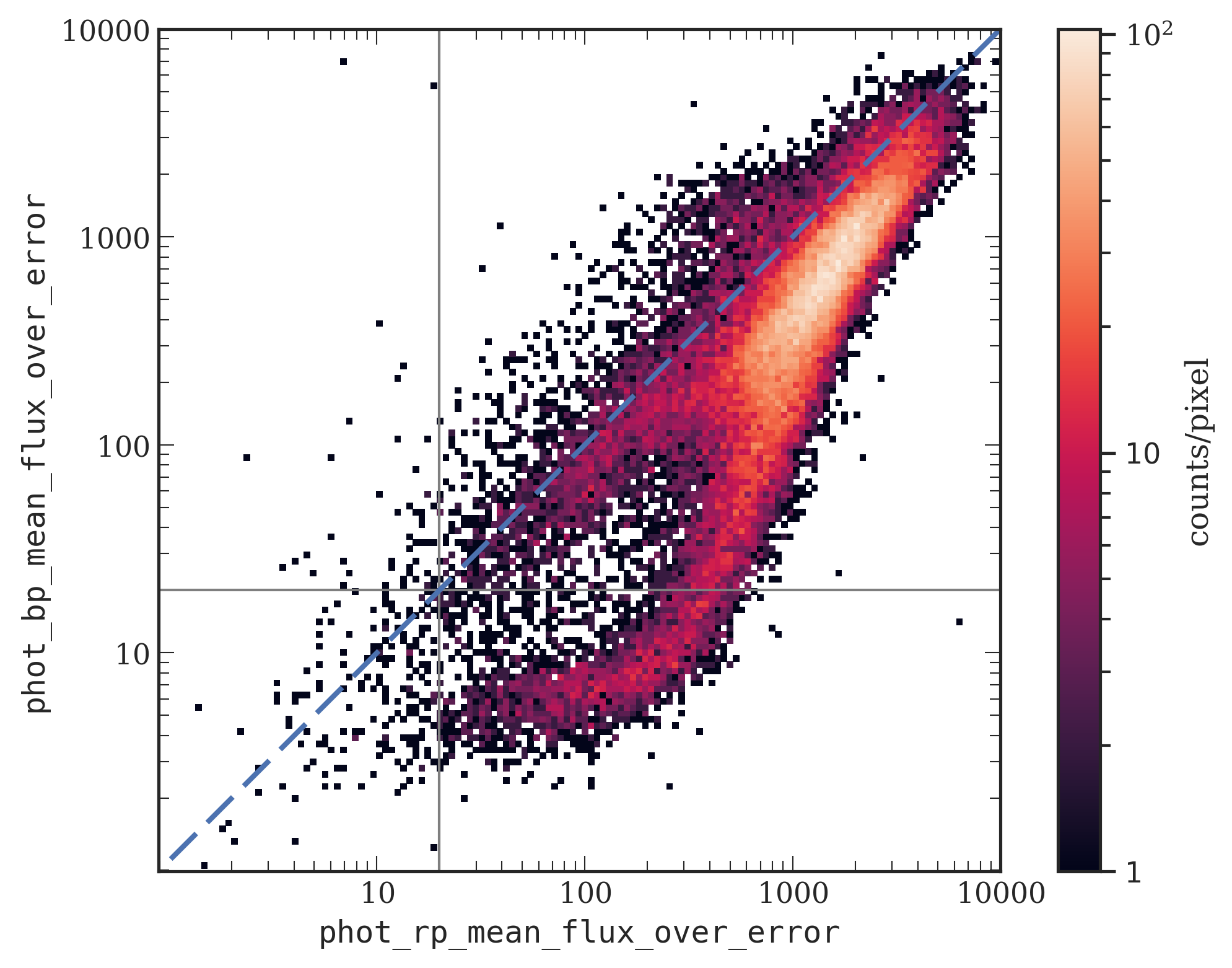
Figure 20: $BP$ and $RP$ flux-over-error ratios for 39 873 sources in a 50 pc sample retained by Eq. (14). The vast majority of objects is located below the 1:1 line (blue dashed line), i.e. the S/N for these objects is higher in the $RP$ band than in the $BP$ band. Grey lines correspond to the S/N threshold applied in Eq. (17). It is noteworthy that there is a significant fraction of objects with high-S/N $RP$ photometry, but low-S/N $BP$ photometry ($S/N_{BP}<20\ \&\ S/N_{RP}>20$).

Here we recall that the $BP$ and $RP$ fluxes are the integrated mean fluxes from the Gaia photometric instrument, and these fluxes are obtained from CCD windows of $3.5^{\prime\prime}\times 2.1^{\prime\prime}$ size downlinked to Earth, whereas the broad-band $G$ flux is determined from PSF or LSF fitting to an object window from the astrometric field (AF) CCDs (Busso et al. 2021).

If there is an additional object in the window of the source (due to, e.g., a crowded field or a binary), the measured flux will be affected by blending and the flux value will be overestimated. This primarily affects $BP$ and $RP$ bands; contamination in the $G$-band is rather infrequent due to the smaller AF window size ($0.72^{\prime\prime}\times 2.1^{\prime\prime}$; Gaia Collaboration et al. 2016).

With this in mind, when using the $G-RP$ colour – that is, combining unbiased $G$ flux with the overestimated $RP$ flux – blended sources or poorly resolved binaries should appear redder than well-behaved single sources, just as observed in a CMD using $G-RP$ on the abscissa.

Affected sources can be identified without prior knowledge of their position in a CMD. For instance, the impact of blending can be assessed with a metric defined as a simple ratio between the total number of blended transits in both $BP$ and $RP$ bands and the total number of observations in these bands (Riello et al. 2021):

$$\beta=\frac{N_{BP_{\rm blended}}+N_{RP_{\rm blended}}}{N_{BP}+N_{RP}},$$ (16)

where $N_{BP_{\rm blended}}$ and $N_{RP_{\rm blended}}$ correspond to the number of transits flagged as blended in the $BP$ and $RP$ bands, respectively (phot_bp_n_blended_transits and phot_rp_n_blended_transits columns in the Gaia EDR3 gaia_source table), while $N_{BP}$ and $N_{RP}$ are the total number of observations that were used to compute the integrated mean flux and its error in the $BP$ and $RP$ bands, respectively (phot_bp_n_obs and phot_rp_n_obs columns in Gaia EDR3).

Furthermore, Gaia EDR3 contains various quality indicators which hint at the possibility that an object is a semi-resolved binary (optical or physical). In particular, ipd_frac_multi_peak corresponds to the percentage of windows where more than one peak was detected by the Image Parameter Determination (IPD) algorithm (Lindegren et al. 2021b).

In Fig. 21 we demonstrate that the outliers discussed above can indeed be attributed to inconsistencies in the photometry of blended objects (top panel) or poorly resolved binaries (bottom panel), or both.

Even though deblending and decontamination is not implemented in Gaia EDR3, it is already now possible to significantly improve the $G-RP$ photometry for blended and contaminated objects.

We start with the following fundamental assumption: while blending biases the measured values of $BP$ and $RP$ fluxes, it results only in negligible changes in their ratio (i.e. $BP-RP$ colour). This holds especially true if the colour of both, the contaminating source and the contaminated source, is similar.

Therefore, the effect of blending can be dramatically reduced by defining a synthetic $G-RP$ colour, which can be derived from an empirical relationship between the $G-RP$ and the $BP-RP$ colour as described in the following.

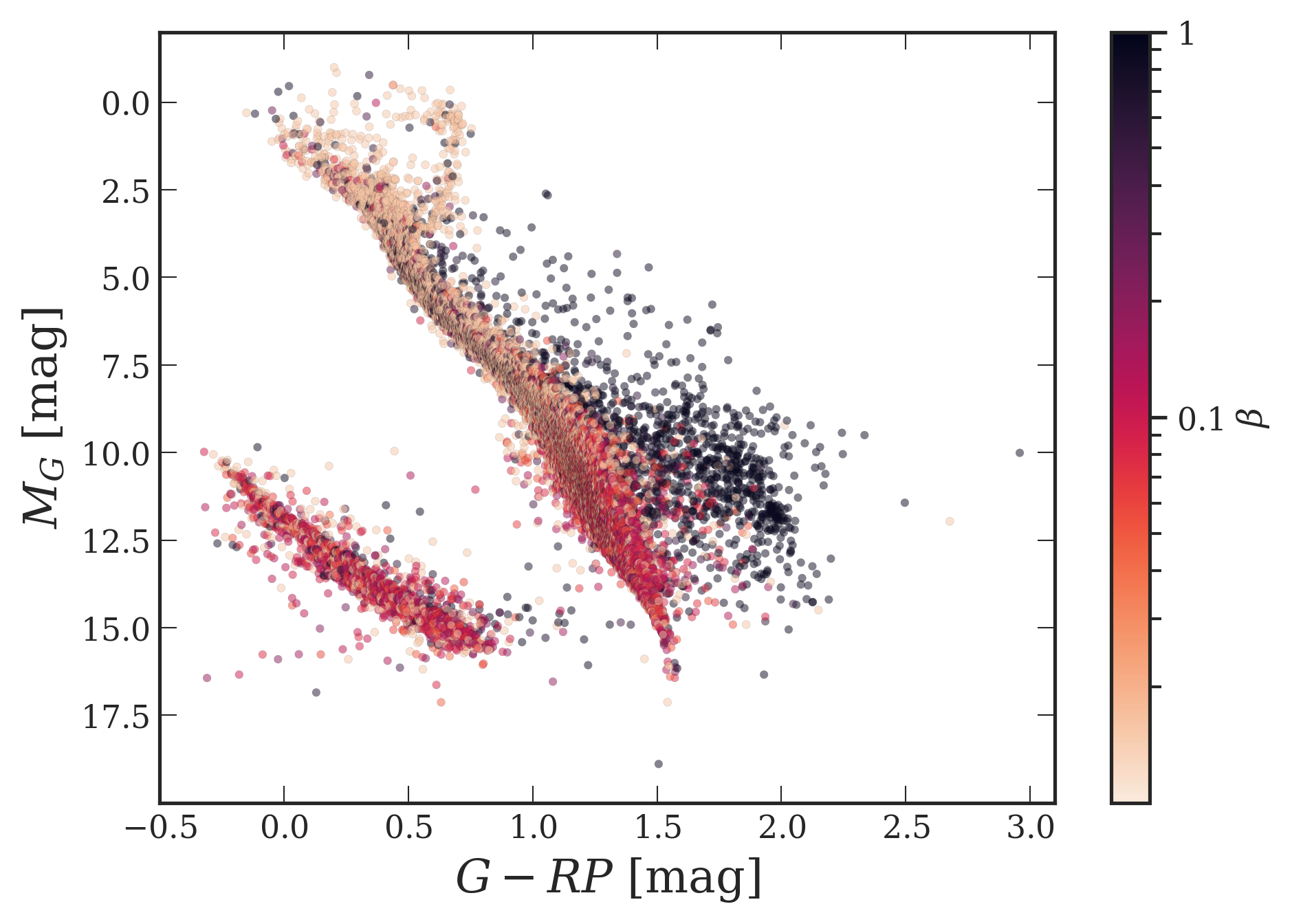
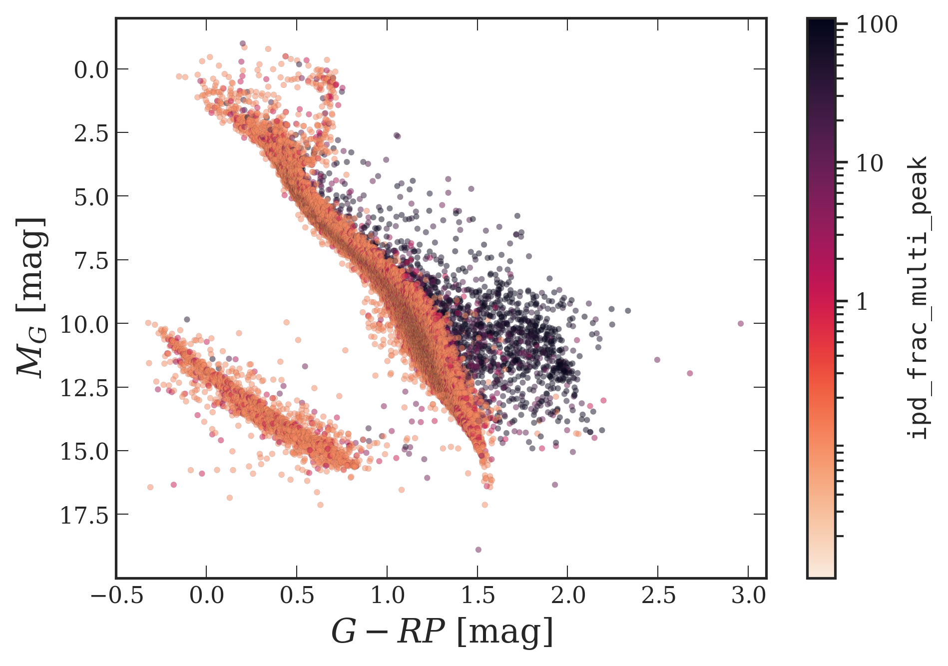
Figure 21: Colour-magnitude diagram for the 50 pc sample colour-coded with the blending metric $\beta$ (top panel) and ipd_frac_multi_peak (bottom panel). Objects with large values of these two metrics exhibit an anomalous location on the diagram. A few extreme outliers are outside of the frame.

In order to derive an empirical relationship between the $G-RP$ and $BP-RP$ colours, we construct a sample of well-behaved objects in Gaia EDR3 with distances up to 100 pc. Here, one wants to use the largest possible sample from Gaia EDR3. However, at larger distances reddening starts to become significant and can bias our calibration. Therefore, we selected only objects with parallaxes larger than 10 mas (corresponds to the distance limit of 100 pc) where reddening is negligible.

For this calibration, it is of fundamental importance to select only objects with excellent photometry, whereas the completeness of the sample is not crucial. Therefore, we apply additional stricter cuts on the astrometrically clean dataset.

We select only sources with high signal-to-noise ratio in both, $BP$ and $RP$ bands ($S/N>20$; the threshold is denoted by the grey lines in Fig. 20). Furthermore, we exclude bright objects severely affected by saturation; namely, we consider only sources with $G>6\leavevmode\nobreak\ {\rm mag}$ (Lindegren et al. 2021b; Riello et al. 2021).

To ensure that we have a sample of excellent data, we select only sources with five-parameter astrometric solutions in Gaia EDR3. In this way we also avoid systematic effects due to the uncertainty of the $G$-band corrections for the sources with six-parameter astrometric solutions (Riello et al. 2021).

Blended sources and (poorly) resolved binaries were removed by applying cuts on the blending metric $\beta$ and the ipd_frac_multi_peak statistic.

Furthermore, we excluded white dwarfs from our sample due to their larger scatter in colour-colour diagram, and limited our sample to colours in the range $0.0\leavevmode\nobreak\ {\rm mag}\leq(BP-RP)\leq 4.25\leavevmode\nobreak\ {\rm mag}$. Outside of this range the data density drops significantly and, consequently, this would yield an unreliable fit for sources with extreme colours.

To summarise, we constructed the initial sample by applying the following selection criteria:

$$\begin{aligned} \text{(i)}\quad&\varpi>10\ \mathrm{mas},\\ \text{(ii)}\quad&\text{Eq.\leavevmode\nobreak\ \eqref{eq:ipd_gof_harm_ampl_cut}:}\ A_{\rm GoF}<10^{-5.12}\leavevmode\nobreak\ (\varpi/\sigma_{\varpi})^{2.61},\\ \text{(iii)}\quad&\texttt{phot\_bp\_mean\_flux\_over\_error}>20,\\ \text{(iv)}\quad&\texttt{phot\_rp\_mean\_flux\_over\_error}>20,\\ \text{(v)}\quad&G>6.0\leavevmode\nobreak\ {\rm mag},\\ \text{(vi)}\quad&\texttt{astrometric\_params\_solved}=31,\\ \text{(vii)}\quad&\beta<0.1,\\ \text{(viii)}\quad&\texttt{ipd\_frac\_multi\_peak}\leq 2.0,\\ \text{(ix)}\quad&G+5\log_{10}(\varpi/100)\leavevmode\nobreak\ {\rm mag}>10.0\leavevmode\nobreak\ {\rm mag}+2.5(BP-RP),\\ \text{(x)}\quad&0.0\leavevmode\nobreak\ {\rm mag}\leq(BP-RP)\leq 4.25\leavevmode\nobreak\ {\rm mag}.\end{aligned}\quad$$ (17)

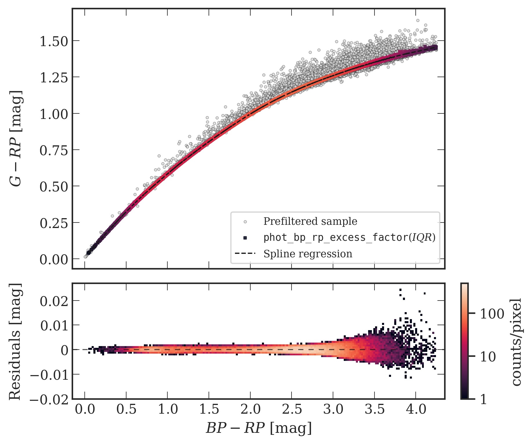
Figure 22: Colour-colour diagram for the prefiltered sample (shown in grey) and the truncated sample, with the colour indicating the number density. The dashed line depicts the model derived using spline regression. The residuals after subtracting the derived relationship are shown in the lower panel.

Finally, in order to obtain a more robust statistics, we construct a truncated sample by using the $BP$ and $RP$ excess factor (phot_bp_rp_excess_factor in the Gaia EDR3 catalogue) for deriving a trimmed estimator. This is done by splitting the initial sample (grey points on Fig. 22, top panel) into bins of 0.005 mag in the $BP-RP$ colour and retaining only objects with $BP$ and $RP$ excess within the interquartile range (IQR) values of phot_bp_rp_excess_factor estimated for each of these bins. There are 91 285 sources in the resulting sample (the coloured part of Fig. 22). The sample contains only sources with high-quality photometry.

In the next step, we derive an empirical model for the synthetic $G-RP$ colour, where input is $BP-RP$ colour. The aim is to mitigate the inconsistencies between $G$ and $RP$ photometry caused by blending or marginally resolved binaries.

To derive the fit of $G-RP$ for isolated well-behaved sources, we use cubic splines with 500 equally spaced knots. Even though 500 knots seems like a large number, this is still an appropriate choice given the large size of our sample (each knot contains on average $\sim 180$ data points). Furthermore, we wish to emphasise that in our case reducing the interpolation error and thus getting smaller residuals has higher priority than avoiding the problem of overfitting.

The residuals of the derived relationship are shown in Fig. 22 (bottom panel). They are very small, do not show any systematics, and illustrate the high quality of the derived relationship. The RMS error is 0.0013 mag.

The derived relationship is applicable in the range $0.0\leavevmode\nobreak\ {\rm mag}<BP-RP<4.25\,\mathrm{mag}$. Another constraint to be considered when applying the relationship is the S/N of $BP$ and $RP$ fluxes in the input. Including sources with a low S/N will lead to unreliable $G-RP$ estimates. Thus, to avoid this, we adopted $S/N=20$ as the optimal threshold value.

To illustrate the power of the suggested correction, CMDs before and after deblending are shown for the 50 pc sample (Fig. 23). The colour-coding indicates the difference between the catalogued and deblended values of $G-RP$. When a CMD is plotted against the catalogued (i.e. uncorrected) $G-RP$ colour values, the objects with large residuals appear mostly at unexpected regions of the diagram (Fig. 23, top panel) and their position in a CMD is not determined by intrinsic properties of an object, but is a consequence of inconsistency in photometry. However, when the deblended colour is used (Fig. 23, bottom panel), they are located in the expected regions of a CMD. Here, we stress that the objects which have peculiar positions in the top panel were not removed, but are plotted with the deblended $G-RP$ colour and are now located on the main sequence, white dwarf sequence, and in the red clump region.

Deblended values of $G-RP$ are listed in the CNS5 for all objects with colours within the applicability range and with sufficient S/N of $BP$ and $RP$ fluxes.

We provide the derived spline coefficients and a python function to calculate deblended $G-RP$ values.

Deblending of colours and magnitudes for objects with inconsistencies in photometry is crucial for correct object classification based on the position in the CMD, estimating effective temperatures and fitting isochrones.

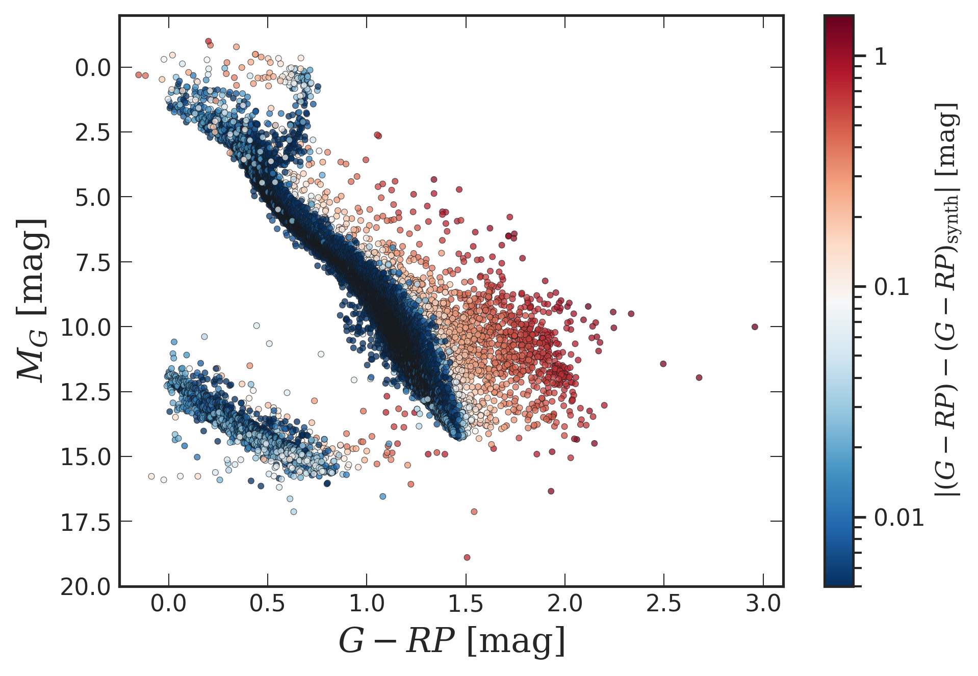
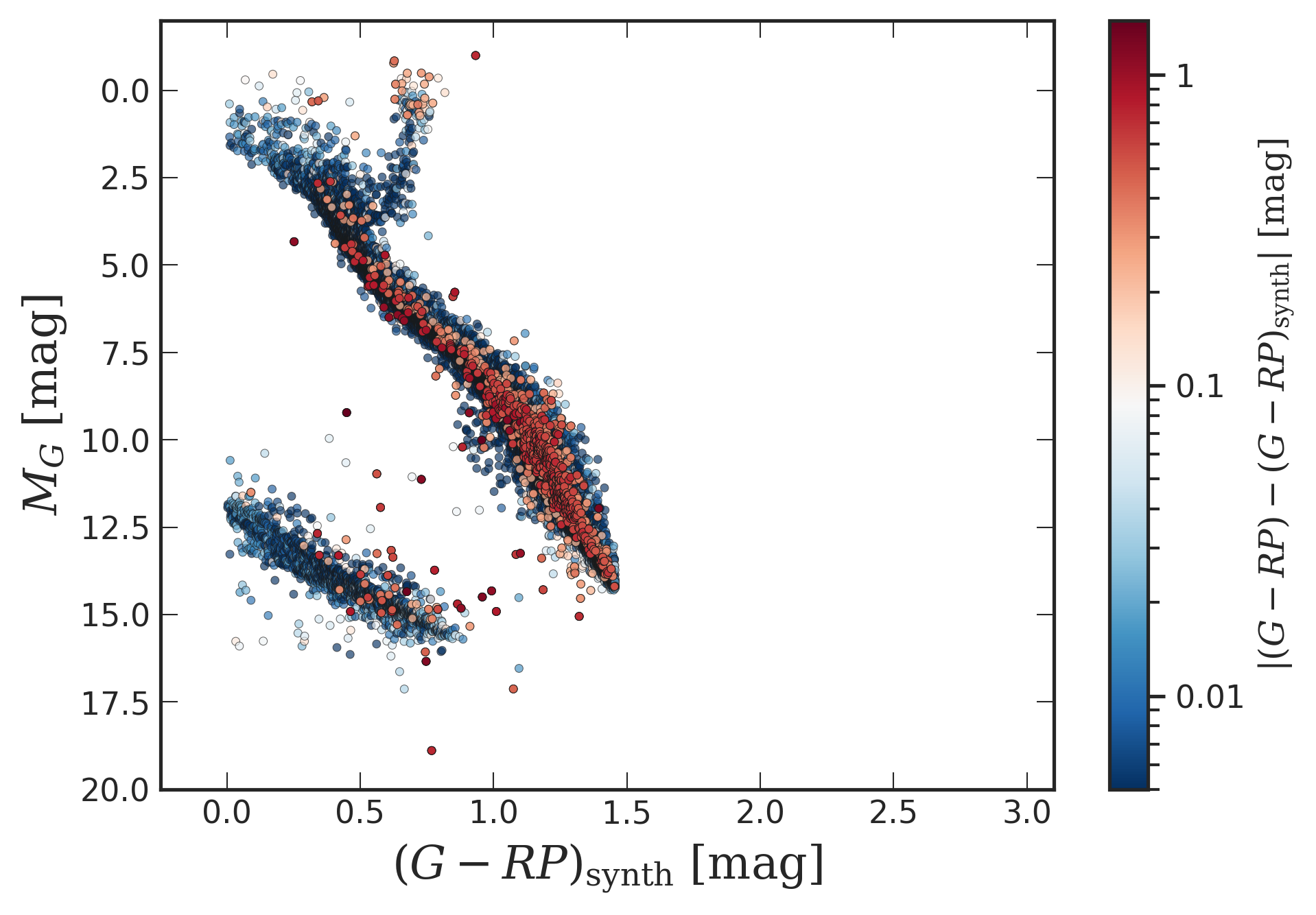
Figure 23: Difference between the measured and deblended $G-RP$ colours for objects in the 50 pc sample and their location on the CMD (using measured $G-RP$ colour). Only objects with $BP-RP$ colours within the applicability range $0.0\leavevmode\nobreak\ {\rm mag}<BP-RP<4.25\leavevmode\nobreak\ {\rm mag}$ are plotted. The colour scale is logarithmic.